Article

Fast Spectral Clustering for Unsupervised Hyperspectral Image Classification

1
Key Laboratory of Spectral Imaging Technology CAS, Xi’an Institute of Optics and Precision Mechanics, Chinese Academy of Sciences, Xi’an 710119, China
2
University of Chinese Academy of Sciences, Beijing 100049, China
3
School of Computer Science and Center for OPTical IMagery Analysis and Learning (OPTIMAL), Northwestern Polytechnical University, Xi’an 710072, China
*
Author to whom correspondence should be addressed.
Remote Sens. 2019, 11(4), 399; https://doi.org/10.3390/rs11040399
Submission received: 16 January 2019 / Revised: 5 February 2019 / Accepted: 12 February 2019 / Published: 15 February 2019
(This article belongs to the Section Remote Sensing Image Processing)

Abstract

:
Hyperspectral image classification is a challenging and significant domain in the field of remote sensing with numerous applications in agriculture, environmental science, mineralogy, and surveillance. In the past years, a growing number of advanced hyperspectral remote sensing image classification techniques based on manifold learning, sparse representation and deep learning have been proposed and reported a good performance in accuracy and efficiency on state-of-the-art public datasets. However, most existing methods still face challenges in dealing with large-scale hyperspectral image datasets due to their high computational complexity. In this work, we propose an improved spectral clustering method for large-scale hyperspectral image classification without any prior information. The proposed algorithm introduces two efficient approximation techniques based on Nyström extension and anchor-based graph to construct the affinity matrix. We also propose an effective solution to solve the eigenvalue decomposition problem by multiplicative update optimization. Experiments on both the synthetic datasets and the hyperspectral image datasets were conducted to demonstrate the efficiency and effectiveness of the proposed algorithm.

Graphical Abstract

1. Introduction

Hyperspectral images (HSIs) contain information on hundreds of continuous narrow spectral wavelengths, which are collected by aircrafts, satellites, and unmanned aerial vehicles in each HSI pixel [1,2,3,4]. Since HSIs reflect rich spectral and spatial resolution, they offer the potential to discriminate more detailed classes and provide even broader applications for land-over classification and clustering [5,6,7,8]. To a certain extent, dealing with HSIs is difficult because the numerous spectral bands significantly increase the computational complexity and the noise in HSIs can badly influence the classification accuracy [9,10]. The existing work reported by most scholars can be roughly divided into two categories according to whether a certain number of training samples are required, as demonstrated in [11,12]: (1) supervised learning named HSI classification; and (2) unsupervised learning named HSI clustering. In the literature, many HSI classification algorithms have been proposed and they have achieved excellent performances. One popular method for HSI classification is to first use dimension reduction and then follow a classifier such as support vector machines [13,14]. Due to the noises and redundancy among spectral bands, many feature extraction, band selection and dimension reduction techniques have been developed in the past years. Some representative work, such as principle component analysis [15] and feature-selection algorithm [16,17], are also widely applied in HSI classification. Kernel-based algorithms such as SVM and its variants [14] have been shown to improve performance [18]. Sparse representation [19] has also been introduced to the task of HSI classification. Newly raised deep learning techniques [20] have proved to be useful for supervised HSI classification.
HSI classification based on supervised methods provides excellent performance on standard datasets (e.g., more than 95% of the overall accuracy) [21]. However, the reported HSI classification algorithms require a certain number of high quality samples to obtain an optimal model. Recently, many researchers noticed that it is expensive or even impossible to collect enough labeled training data in some cases, and some recent work pay more attention to the problem of “small sample size” and present encouraging results, e.g., semi-supervised learning [22], active learning [23], domain adaptation [24], and tensor learning [25]. Although these methods could achieve similar classification results as supervised ones while using fewer training samples, they are still supervised methods that require high quality training samples to learn the classification model. On the contrary, clustering-based techniques require little prior knowledge and can be considered as data preprocessing methods to provide necessary reference information regarding supervised classification, target detection, or spectral unmixing. Therefore, unsupervised HSI classification is an extremely important techniques and has attracted significant attention in recent years. Wang et al. [26] illustrated that the existing algorithms can be coarsely divided into the following four categories: (1) Centroid-based clustering methods, such as k-mean [27] and fuzzy c-means [28], minimize the within cluster sample distance, but are sensitive to initialization and noise, and cannot provide a robust performance. (2) Density-based methods include the clustering by fast search and find the density peak algorithm [29], the density-based spatial clustering of applications with noise [30], and the clustering-in-quest method [31], which are not suitable for HSIs as it is difficult to get the density peak in the sparse feature space. (3) Biological clustering methods include the artificial immune networks for unsupervised remote sensing image classification [32] and the automatic fuzzy clustering method based on adaptive multiobjective differential evolution [33]. Their results are not always satisfactory because biological models do not always exactly fit the characteristics of HSIs. (4) Graph-based methods, such as spectral clustering [34,35], perform well in the task of unsupervised HSI classification but most of them take too much time on the eigenvalue decomposition and the affinity matrix.
In general, the accuracy of the existing unsupervised HSI classification algorithms are far from satisfactory compared to the supervised techniques due to the uniform data distribution caused by the large spectral variability. In this paper, we focus on the family of graph-based clustering algorithms (i.e., spectral clustering algorithms) [36,37]. Compared with other clustering techniques, spectral clustering has good performance in dealing with irregularly-shaped clusters and gradual variation within groups. In general, spectral clustering performs a low-dimension embedding of the affinity matrix followed by a k-means clustering in the low-dimensional space [38]. The utilization of graph model and manifold information makes it possible to process the data with complicated structure. Accordingly, algorithms based on spectral clustering have been widely applied and shown their effectiveness in the task of HSI processing. Although the spectral clustering methods have performed well, it would be too expensive to calculate the pairwise distance of enormous samples and difficult to provide an optimal approximation for eigenvalue decomposition in dealing with a large affinity matrix. In the clustering process, the complexity mainly arises from two aspects. First, the storage complexity of the affinity matrix is O ( n 2 ) and the corresponding time complexity is O ( n 2 d ) . The second is the eigenvalue decomposition of Laplacian matrix, which is O ( n 2 c ) time complexity. Note that n, d, and c are the number of pixels, feature dimensions, and classes of HSI, respectively. It is obvious that high spatial resolution (i.e., number of pixels n) is a major constraint to apply spectral clustering to real-life HSI applications. In our experiments, spectral clustering techniques can be applied to small-scale HSI datasets such as Samson, Jasper, SalinasA, and India Pines, as these datasets contain only about 10,000 pixels. However, along with the increase of spatial resolution of HSIs, it could be unacceptable for the large-scale HSI datasets including Salinas, Pavia University, Kennedy Space Center, and Urban, which contain about 100,000 pixels, because of the rapid growth of the storage and time complexity of affinity matrix construction and eigenvalue decomposition of Laplacian matrix.
To alleviate the above problem, several improved spectral clustering methods have been proposed for large-scale HSIs with high spatial resolution. An efficient way to get low-rank matrix approximation based on Nyström extension has been widely applied in many kernel based clustering task [39,40], and recent studies have shown good performance in the task of HSI processing [41,42]. Another method proposed by Nie et al. [43,44] constructs anchor-based affinity matrix with balanced k-means based hierarchical k-means algorithm. Wang et al. [26] improved the anchor-based affinity matrix by incorporating the spatial information. Meanwhile, Nonnegative Matrix Factorization (NMF) technique [45,46] and its variants also provide an efficient solution for HSI classification. Motivated by the existing approaches, we propose an improved spectral clustering based on multiplicative update algorithm and two efficient methods for affinity matrix approximation. In general, the spectral clustering problem can be solved by the standard trace minimization of the objective function and we propose an efficient resolution though multiplicative update optimization according to the derivative of the objective function. Meanwhile, the nonnegative constraint and the orthonormal constraint provide a better indicator matrix and this makes it easier to get a robust clustering result by the later processing such as k-means. Furthermore, the anchor-based graph and the Nyström extension are introduced to improve the computational complexity by affinity matrix approximation for the large-scale HSIs. There are three main contributions of this work:
  • An novel multiplicative update optimization for eigenvalue decomposition is proposed for large-scale unsupervised HSIs classification. It is worth noting that the proposed method can be easily portable to the variants of spectral clustering methods with different regularization items only if the constraints are convex functions.
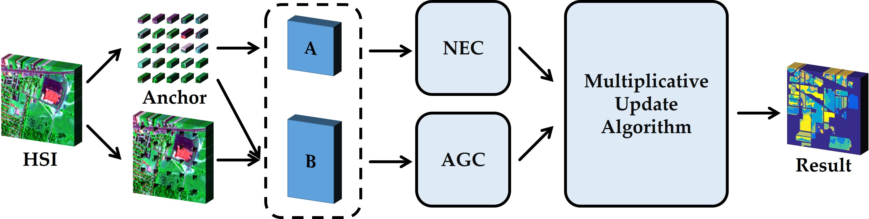
  • Two affinity matrix approximation techniques, namely the anchor-based graph and the Nyström extension, are introduced to improve the affinity matrix by sampling limited samples (i.e., pixels or anchors).
  • Comprehensive experiments on the HSI datasets illustrated that the proposed method achieved a good result in terms of efficiency and effectiveness, and the combination of multiplicative update method and affinity matrix approximation provided a better performance.
The rest of this paper is organized as follows. Section 2 provides notations and a brief view of the general spectral clustering algorithm. Next, we present the motivation and formulate the proposed multiplicative update algorithm. Furthermore, an effective multiplicative update method for eigenvalue decomposition is presented in Section 3. To further improve the computational complexity of affinity matrix, we introduce two efficient approximated techniques in Section 4. The experimental results including performance analyses, computational complicity and parameter determination are given in Section 5. Section 6 concludes this paper.

2. Overview

We begin by reviewing the classical spectral clustering algorithm, and before going into the details, we firstly introduce the notation.

2.1. Notation

In this part, we define some notation to make sure that the mathematical meaning of the proposed method can be formulated clearly. The pixels of HSIs can be considered as { x i R d , i = 1 , 2 , , n } where d is the dimensionality (i.e., the number of spectral bands). Let { y 1 , y 1 , , y c } R c be the indicator vectors of the pixels { x 1 , x 1 , , x n } , respectively. Here, y i = [ y i 1 , y i 2 , , y i c ] , where c is the predefined number of clusters, and the indicator vectors y i j = 1 if and only if x i belongs to the jth cluster and y i j = 0 otherwise. Denote Y = [ y 1 T , y 2 T , , y n T ] T R n × c , and Y 0 indicates that the whole elements of Y are nonnegative. The affinity matrix is denoted by W and the Laplacian matrix is denoted by L . The corresponding trace can be denoted by Tr ( W ) and the Frobenius norm of W is denoted by | | W | | F . The detailed notations are summarized in Table 1 and we explain the meaning of each term when it is first used.

2.2. Normalized Cuts Revisit

A set of samples (i.e., pixels) { x 1 , x 2 , , x n } can be considered as an undirected graph G = { V e r t i c e s , E d g e s } . Each vertex represents a sample x i and the edge is aligned by their similarity. In general, the corresponding affinity (or similarity) matrix W can be denoted as
W i j = e | | x i x j | | 2 2 2 σ 2 , i , j = 1 , 2 , , n ,
where σ is the width of the neighbors, W is a symmetric matrix and W i j is the affinity of samples x i and x j . Let A and B represent a bipartition of V e r t i c e s , where A B = V e r t i c e s and A B = . Let  cut ( A , B ) denotes the sum of the weights between A and B as cut ( A , B ) = i A , j B W ij . The volume of a set is defined as the sum of the degrees within that set: vol ( A ) = i A D i i and vol ( B ) = i B D i i , where D i i = j W i j . The normalized cut between A and B can be considered as follows:
NCut ( A , B ) = cut ( A , B ) vol ( A ) + cut ( A , B ) vol ( B ) = 2 cut ( A , B ) vol ( A ) | | vol ( B ) ,
where | | is the harmonic mean. According to [47], an optimal resolution of NCut ( A , B ) can be provided by solving the minimization of the following equation
min y T ( D W ) y y T D y = min y T D 1 2 ( D W ) D 1 2 y ,
where D is the diagonal matrix with elements D i i = j W i j . y is the indicator vector, where y i j = 1 if and only if x i belongs to the jth cluster and y i j = 0 otherwise.
According to spectral graph theory, an approximate resolution of Equation (3) can be considered as thresholding the eigenvector corresponding to the second smallest eigenvalues of the normalized Laplacian L as follows:
L = D 1 2 ( D W ) D 1 2 = I D 1 2 W D 1 2 .
Shi and Malik [47] illustrated that the normalized Laplacian matrix L is positive semidefinite even when W is indefinite. Its second smallest eigenvalue lies on the interval [ 0 , 2 ] so the corresponding eigenvalues of D 1 2 W D 1 2 are confined to lie inside [−1, 1]. Considering the case of multiple group clustering where c > 2 , Equation (3) can be rewritten as
min Tr ( Y T L Y ) ,
where Y T Y = I and Y is the indicator matrix. This can be solved by the standard trace minimization problem according to the normalized spectral clustering proposed in [47]. The solution Y consists of the top c eigenvectors of the normalized Laplacian matrix L as columns.
However, there are two tough problems to get an efficient and effective solution by using the classical spectral clustering technique: one is the eigenvalue decomposition of the Laplacian matrix L, which takes O ( n 2 c ) time complexity, and the other one is the storage and time complexity of the affinity matrix, which are O ( n 2 ) and O ( n 2 d ) , respectively. It is obvious that either of the above problems can be an unbearable burden with the increasing of the number of samples. To alleviate the above problem, motivated by the recent work such as Nyström extension, anchor-based graph and nonnegative matrix factorization, we propose a novel approach to solving the large-scale and high-dimensional HSI clustering (or unsupervised HSI classification), and the detailed demonstration are presented in the following sections.

3. Improved Spectral Clustering with Multiplicative Update Algorithm

In this section, we propose an multiplicative update algorithm to get an efficient resolution of the eigenvalue decomposition of the Laplacian matrix L. We firstly present the formulation and our motivation, and then a novel resolution for spectral clustering based on multiplicative update algorithm is proposed in Section 3.2.

3.1. Formulation and Motivation

In general, a multigroup spectral clustering problem (i.e., c > 2 ) can be considered as a minimization of the following equation:
min Tr ( Y T L Y ) + λ | | Y T Y I | | F 2 ,
where λ > 0 is the Lagrangian multiplier and | | Y T Y I | | F 2 is the item for orthonormal constraint. However, Equation (6) is still a non-smooth objective function, thus it is difficult to obtain an efficient resolution by solving the eigenvalue decomposition of the Laplacian matrix L. Motivated by NMF, which has excellent performance in dealing with clustering by relaxation technique, we relax the discreteness condition and propose an multiplicative update optimization to solve the eigenvalue decomposition, the details of which are illustrated in the next section.

3.2. Multiplicative Update Optimization

Spectral clustering cannot provide an efficient resolution since it would be too expensive to get an optimal approximation for eigenvalue decomposition in deal with large-scale datasets. Motivated by the recent work on NMF, we introduce the nonnegative constraint for indicator matrix as Y where Y i j > 0 . Moreover, the traditional spectral relation approaches relax the indicator matrix Y to orthonormal constraint as Y T Y = I . According to a recent work [48], if the indicator matrix Y is orthonormal and nonnegative simultaneously, only one element is positive and the others are zeros in each row of Y . Note that we can get an ideal indicator matrix Y as defined in Section 2.1 by considering the above two constraints: Y > 0 and Y T Y = I . The above constraints are significant, which can help us to solve the eigenvalue decomposition in a more efficient way and this is also easy to implement.
By relaxing the discreteness condition and considering the above two constraints, Equation (6) can be rewritten as
min Tr ( Y T L Y ) + λ ( Y T Y I ) = min Tr ( Y T L Y ) + λ Tr ( ( Y T Y I ) T ( Y T Y I ) ) ,
where Y > 0 . Equation (7) can be considered as the cost function and we try to find an optimal resolution of minimization. The derivation of Equation (7) is
L Y + 2 λ Y Y T Y 2 λ Y ,
where L = I D 1 2 W D 1 2 and Equation (8) can be rewritten as
( I D 1 2 W D 1 2 ) Y + 2 λ Y Y T Y 2 λ Y = Y D 1 2 W D 1 2 Y + 2 λ Y Y T Y 2 λ Y = ( Y + 2 λ Y Y T Y ) ( 2 λ Y + D 1 2 W D 1 2 Y ) .
In this case, the derivation of Equation (7) is divided into two parts. Both Y + 2 λ Y Y T Y and 2 λ Y + D 1 2 W D 1 2 Y are nonnegative matrices since Y > 0 , D > 0 , and W 0 . For convenience, we denote the former factor as Q = Y + 2 λ Y Y T Y and the latter factor as P = 2 λ Y + D 1 2 W D 1 2 Y . According the multiplication update rule for standard NMF algorithm [49], we can get the minimization of the cost function in Equation (7) by updating Y as follows:
Y Y P Q ,
where ∘ and ⊘ denote Hadamard product and Hadamard division (i.e., element-wise multiplication and division), respectively, and Y i j Y i j · P i j / Q i j . Then, we can get a optimal resolution until the cost function converge and the implement details are presented in Algorithm 1. Since only one element is positive and the others approximate zero in each row of the indicator matrix Y , it can be considered as a nearly perfect indicator matrix for clustering representation.
Algorithm 1: Algorithm to solve the problem in Equation (6).
Remotesensing 11 00399 i001

4. Approximated Affinity Matrix

To further improve the time and storage complexity of computing affinity matrix to make the spectral clustering algorithm available for large-scale datasets such as HSIs, we introduce anchor-based graph and Nyström extension to approximate the original affinity matrix with limited samples.

4.1. Affinity Matrix with Nyström Extension

The Nyström extension is a technique for finding numerical approximations to eigenfunction problems and the detailed illustration can be found in [50]. It allows us to extend an eigenvector computed for a set of sample points to arbitrary samples x with the interpolation weights.
Inspired by [47], the affinity matrix considers both the brightness value of the pixels and their spatial location, and we can define the similarity of two samples x i and x j as
W i j = e | | l i l j | | 2 2 2 σ l 2 · e | | x i x j | | 2 2 2 σ x 2 ,
where l i and l j are the spatial locations of the HSI’s pixels. σ l and σ x are the bandwidth of neighboring pixels and these parameters are sensitive to different HSIs. To alleviate this problem, Zhao et al. [35] introduced an adaptive parameter and we can define σ ¯ l and σ ¯ x as
σ ¯ l 2 = 1 n 2 i = 1 n j = 1 n | | l i l j | | 2 2 , σ ¯ x 2 = 1 n 2 i = 1 n j = 1 n | | x i x j | | 2 2 .
and Equation (11) can be presented as
W i j = e | | l i l j | | 2 2 2 α σ ¯ l 2 · e | | x i x j | | 2 2 2 α σ ¯ x 2 .
where the parameter α controls the neighbor of affinity matrix.
For uniformity in notation, the affinity matrix A is similarity defined by Equation (11) of m chosen samples. The affinity matrix of the remaining n m samples and the chosen samples are denoted as B . C is the affinity matrix for the remaining samples. The affinity matrix W can be rewritten as
W = A B B T C ,
where A R m × m , B R m × ( n m ) and C R ( n m ) × ( n m ) . According to the Nyström extension, C can be denoted by C = B T A 1 B and the approximated affinity matrix W can be formulated as
W ^ = A B B T B T A 1 B = A B T A 1 A B .
We can find that the size of this norm is governed by the extent to which C is spanned by the rows of B , and the Nyström extension provides an approximation to the entire affinity matrix with only a subset of rows or columns.
To extend the above matrix form of Nyström method to NCut, we need to calculate the row sum of matrix W ^ . However, it is possible without explicitly evaluating the sub-matrix B T A 1 B since
d = W ^ 1 = A 1 m + B 1 n B T 1 m + B T A 1 B 1 n ,
where A 1 m and B 1 n are the row sum of matrix A and A and B T 1 m is the column sum of matrix B . Then, the matrix A and B can be formulated as
A i j A i j d i d j , B i j B i j d i d j + m ,
and we can get the normalized affinity matrix D 1 2 W ^ D 1 2 (refer to Equation (15)) as before; thus, we can get
D 1 2 W ^ D 1 2 = A B T A 1 A B ,
where A and B are from Equation (17). However, the elements of D 1 2 W ^ D 1 2 can be negative since the matrix A 1 may contain negative elements. However, we have to keep D 1 2 W ^ D 1 2 0 to satisfy the constraints of the proposed multiplicative update algorithm. Because of this, we denote A + = ( | A | + A ) . / 2 and A = ( | A | A ) . / 2 , where we can find that A + is the positive part of A and A is the negative part of A . Note that both A + and A are negative matrix and P and Q can be formulated as
P = A B T A + A B Y + 2 λ Y , Q = A B T A A B + Y + 2 λ Y Y T Y .

4.2. Affinity Matrix with Anchor-Based Graph

The anchor-based graph was proposed by Zhu et al. [43] for large-scale data clustering problem. It makes the label prediction function a weighted average of the labels on a subset of anchor samples. If one can infer the labels of other unlabeled samples, they are easily obtained by a simple linear combination. As such, the label prediction function f ( · ) can be represented by a subset A = { a j } j = 1 m R D in which each a j acts as an anchor sample,
f ( x i ) = j = 1 m Z i j f ( a j ) ,
where Z is the data-adaptive weight matrix which measures the similarity between samples and anchors. We define two vectors F = [ f ( x 1 ) , f ( x 2 ) , , f ( x n ) ] T and F a = [ f ( a 1 ) , f ( a 2 ) , , f ( a n ) ] T , thus Equation (20) can be rewritten as
F = Z F a , Z R n × m , m n .
This formula reduces the solution space of unknown labels from large F to smaller F a .
The first problem of anchor-based graph construction is how to choose the anchors. In general, the anchors can be considered as random samples or representative samples such as k-means clustering centers. Random selection chooses m anchors by random sampling from samples with computational complexity O ( 1 ) . However, the randomly chosen samples cannot guarantee that the approximated affinity matrix is always robust. Liu et al. [51] suggested using k-means clustering centers as anchors instead of randomly chosen samples since the k-means clustering centers have a robust representation power to adequately cover the whole data. However, the computational complexity of k-means is O ( n d m t ) , where t is the number of iterations.
The second problem is how to design a regression matrix Z that measure the underlying relationship between the whole samples and the chosen anchors. Liu et al. [51] proposed a method named Local Anchor Embedding (LAE) to reconstruct the regression matrix, where { a 1 , a 2 , , a m } denote the chosen anchors and K ( · ) is a given kernel function with bandwidth parameters:
Z i j = K ( x i , a j ) k Φ i K ( x i , a k ) , j Φ i
The notation Φ i [ 1 , 2 , , m ] is the set saving the indexes of s nearest neighbors of x i in A , and the Gaussian kernel K ( x i , a j ) = exp ( | | x i a j | | 2 2 / 2 σ 2 ) is adopted for the kernel regression. However, the kernel-based methods need an extra parameter (i.e., bandwidth σ ). Nie et al. [27] adopted a parameter-free yet effective neighbor assignment strategy and they obtained the ith row of Z by solving following problem:
min Z i T 1 = 1 , Z i 0 j = 1 m | | x i a j | | 2 2 Z i j + γ Z i j 2 ,
where Z i T denotes the ith row of Z and γ is the regularization parameter. Note that Equation (23) does not consider the spatial information of HSIs, which may result in some isolated pixels appearing in the clustering HSI due to the existence of noise, outliers, or mixed pixels. Recent studies incorporate the spatial information by directly modifying the cost function in Equation (23) as follows:
min Z i T 1 = 1 , Z i 0 j = 1 m | | x i a j | | 2 2 Z i j + β | | x ¯ i a j | | 2 2 Z i j + γ Z i j 2 ,
where x ¯ i is the mean of the neighboring pixels lying within a window around x i and the parameter α controls the tradeoff between hyperspectral information and spatial information. Let d i j x = | | x i u j | | 2 2 and d i j x ¯ = | | x ¯ i u j | | 2 2 , and denote d i R m a vector with the jth element as d i j = d i j x + β d i j x ¯ . It is obvious that Equation (24) can be rewritten in vector form as
min Z i | | Z i + 1 2 γ d i | | 2 2 ,
where Z i T 1 = 1 and Z i 0 . Following y Nie et al. [43], the parameter γ can be denoted by γ = ( s / 2 ) d i , s + 1 ( 1 / 2 ) j = 1 s d i j , and the resolution of Equation (25) is
Z i j = d i , k + 1 d i j k d i , k + 1 j = 1 k d i j .
For the detailed deviation, see [27]. After we get the regression matrix Z , the affinity matrix W can be obtained as
W ^ = Z Δ 1 Z T ,
where Δ is a diagonal matrix, the jth entry is defined as i = 1 n Z i j and W ^ is symmetric positive semidefinite and doubly stochastic. Not that Z i T 1 = 1 and Z i 0 , and it can be verified that W ^ is a double stochastic matrix and W ^ i j 0 . More importantly, the approximated matrix W ^ is automatically normalized and we can find that W ^ = D 1 2 W D 1 2 . In this case, the Laplacian matrix L can be considered as L = I W ^ and we can rewrite P and Q as follows:
P = 2 λ Y + Z Δ 1 Z T Y Q = Y + 2 λ Y Y T Y

5. Experiments

In the experiments, we verified the performance of the proposed unsupervised HSI classification algorithm on both synthetic datasets and HSI datasets, and then showed several useful analysis. The synthetic benchmark datasets were three sets of data with manifold structure and the HSI datasets are several hyperspectral images (i.e., Salinas, Pavia University, Kennedy Space Center, Samson, Indian Pines, Urban and Japser).

5.1. Experimental Datasets

We conducted experiments on eight widely used hyperspectral datasets:
  • Salinas and Salinas-A were acquired by the 224-band AVIRIS sensor over Salinas Valley, California, and characterized by high spatial resolution (3.7-m pixels). Salinas covers 512 lines by 217 samples at as scale of 512 × 217 . Salinas ground truth contains 16 classes. Salinas-A is an small subscene of Salinas image and it comprises 86 × 83 pixels located within the same scene at [samples, lines] = [591–676, 158–240] and includes six classes.
  • Pavia University is the scene collected by the ROSIS sensor during a flight campaign over Pavia, northern Italy. The number of spectral bands is 103 for Pavia University. Pavia University is a 610 × 610 pixels image, where some pixels contain no information and these samples are discarded. Both hyperspectral image ground truths differentiate nine classes.
  • Kennedy Space Center was acquired by the NASA AVIRIS instrument over the Kennedy Space Center (KSC), Florida, on 23 March 1996. They acquired data in 224 bands of 10 nm width with center wavelengths from 400 to 2500 nm and 176 bands were used for the analysis. KSC hyperspectral image contains 512 × 614 pixels. For classification purposes, 13 classes representing the various land cover types that occur in this environment were defined for the site.
  • Samson dataset is an image with 95 × 95 pixels and each pixel was recorded at 156 channels covering the wavelengths from 401 nm to 889 nm. The spectral resolution is high up to 3.13 nm and it is not degraded by blank or noisy channels. There are three targets in this image: Soil, Tree and Water.
  • Japser Ridge is a hyperspectral image with 100 × 100 pixels. Each pixel was recorded at 224 channels ranging from 380 nm to 2500 nm. The spectral resolution is up to 9.46 nm. There are four end-members latent in these data: Road, Soil, Water and Tree.
  • Urban has 210 wavelengths ranging from 400 nm to 2500 nm, resulting in a spectral resolution of 10 nm. There are 307 × 307 pixels, each of which corresponding to a 2 × 2 m 2 area. There are three versions of the ground truth, which contain 4, 5 and 6 end-members respectively, and are introduced in the ground truth.
  • Indian Pines was gathered by AVIRIS sensor in northwestern Indiana and consists of 145 × 145 pixels and 224 spectral reflectance bands. The Indian Pines scene contains two-thirds agriculture, and one-third forest or other natural perennial vegetation. The ground truth available is designated into sixteen classes and we reduced the number of bands to 200 by removing bands covering the region of water absorption.

5.2. Evaluation Metrics

In the experiments, we evaluated the clustering results by Purity (P.) and Normalized Mutual Information (NMI).
  • P. is the most common metric for clustering results evaluation and it can be formulated as
    Purity ( Ω , Ω ^ ) = 1 n i max j | Ω i Ω ^ j |
    where Ω is the clustering result set and Ω ^ is the ground truth. The worst clustering result is very close to 0 and the best clustering result has a purity value equal to 1.
  • NMI is a normalization of the mutual information score to scale the results between 0 and 1 as
    NMI = i = 1 c j = 1 c n i , j l o g n i , j n i n ^ j ( i = 1 c n i l o g n i n ) ( i = 1 c n ^ i l o g n ^ i n ) ,
    where n i denotes the number of data contained in the cluster C i ( 1 i c ) , n ^ j is the number of data belonging to the L j ( 1 j c ) , and n i , j denotes the number of data that are in the intersection between the cluster C i and the class L j . The larger is the NMI, the better is the clustering result.
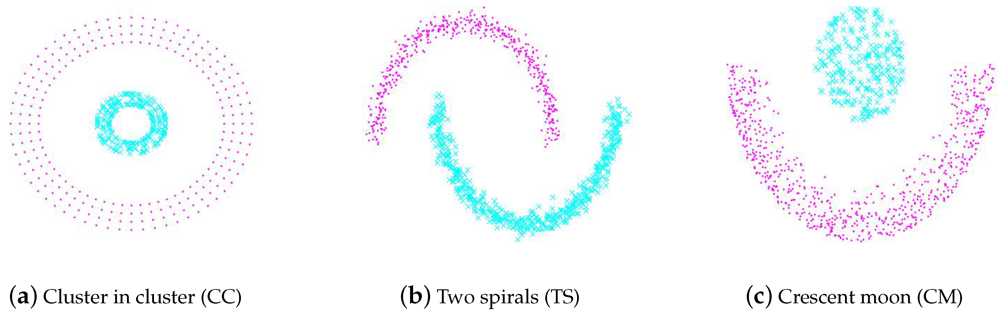
We ran the experiments under the same environment: Intel(R) Core(TM) i7-5930K CPU, 3.50 GHz, 64 GB memory, Ubuntu 14.04.5 LTS system and Matlab version R2014b. We compared our algorithm with Spectral Clustering (SC), Anchor-based Graph Clustering (AGC), and Nyström Extension Clustering (NEC). The corresponding improved algorithms based on multiplicative update optimization are SC-I, NEC-I, and AGC-I. The affinity matrix of the above algorithms were constructed in three ways and the detailed description of the above affinity matrix is presented in the next section.

5.3. Toy Example

We firstly explored the performance of our algorithm on three synthetic datasets to verify the effectiveness of multiplicative update optimization and two approximated affinity matrix matrices. In this experiment, three synthetic datasets were introduced in our experiment: Cluster in Cluster (CC), Two Spirals (TS), and Crescent Moon (CM). Figure 1 presents the manifold structure of the synthetic datasets in detail. These synthetic datasets contain 2000–40,000 data points that are divided into two groups and they are extremely challenging since clustering algorithms that only consider data point distance have difficulty obtaining a robust result. The algorithms with spectral graph theory provide a more powerful technique in dealing with the manifold information. The resolution for spectral clustering can be divided into two parts: affinity matrix construction and eigenvalue decomposition of the Laplacian matrix. In this paper, we present three formulations for the affinity matrix construction as
Euclidean distance : W i j = e | | x i x j | | 2 2 2 α σ ¯ 2 , Nystr ö m extension : W ^ = A B T A 1 A B , A i j = e | | u i u j | | 2 2 2 α σ ¯ 2 , B i j = e | | u i x j | | 2 2 2 α σ ¯ 2 , Anchor - based graph : W ^ = Z Δ 1 Z T , Z i j = d i , k + 1 d i j k d i , k + 1 j = 1 k d i j .
where x is the whole sample and u is the chosen data points. α is the parameter to control the neighbor of data points for Euclidean distance and we set α = 10 . A is the affinity matrix for anchors (chosen data points) and B stores the similarity between anchors (chosen data points) and the remaining ones. d i j denotes the distance between the ith data point and the jth anchor, which can be considered as chosen data points, and d i 1 , d i 2 , , d i n are ordered from small to large. According to [27], the parameter k for anchor-based graph was set to 10, which provided a good performance in most cases. Note that the last two affinity matrices are the approximated solution for the original affinity matrix. The sample scale was set to 10, which means we randomly selected one-tenth of data points as the anchors or the chosen data points.
Compared with the traditional eigenvalue decomposition of the Laplacian matrix, we propose a multiplicative update optimization to get a more efficient solution of eigenvalue decomposition. In our experiments, the number of iterations was about 150 and we obtained good results in most cases. Besides the above-mentioned parameters, the other parameters of the compared algorithms and our improved algorithms were tuned to the optimum.
Table 2, Table 3 and Table 4 present the performance of the above six methods on three synthetic datasets. SC and SC-I provided a good clustering result since the corresponding affinity matrix considered the similarity of the whole data points; however, these two methods also needed more time to calculate the Euclidean distance among samples. Note that the proposed multiplicative update algorithm delivered a substantial efficiency increase, taking only half the time to get a similar clustering result. NEC and AGC had the benefit of the approximated affinity matrix and took only about one-tenth the time, but NEC was not robust enough to get a stable resolution of the eigenvalue decomposition. Compared with NEC, the improved algorithm NEC-I provided a better clustering result because of the orthonormal constraint and nonnegative constraint. AGC performed better than SC and NEC in terms of effectiveness and efficiency in the experiments, as it utilized the anchor-based affinity matrix, and the proposed AGC-I also had a good performance.

5.4. HSI Clustering Analysis

In this section, a further study is presented to illustrate the performance of the proposed multiplicative update algorithm and the efficiency of the approximated affinity matrix mentioned in Section 4 on several popular hyperspectral image datasets. We followed the experiment setting in the previous section where the parameter α was set to 10 and the parameter k was set to 10. In addition, the parameter λ was set to 0.5 and the other parameters were tuned to the optimum for fair competition. Note that the affinity matrix for the hyperspectral image datasets was different from the previous section because it needed to consider both the brightness value and the spatial information. In this case, the affinity matrix W can be rewritten as
W i j = e | | x i x j | | 2 2 2 α σ ¯ x 2 | | l i l j | | 2 2 2 α σ ¯ l 2 ,
where l is the pixel location and the parameter α was set to 10 for both the brightness value and the spatial information. The affinity matrices A and B for NEC were constructed in the same way. Meanwhile, The affinity matrix for AGC is provided as
W ^ = Z Δ 1 Z T , Z i j = d i , k + 1 d i j k d i , k + 1 j = 1 k d i j ,
where d i j = | | x i u j | | 2 2 + | | x ¯ i u j | | 2 2 and x ¯ is the mean of the brightness value around pixel x .
Figure 2 and Table 5 present the experimental results, which were evaluated by Purity and NMI on the hyperspectral image datasets. We made the following observations:
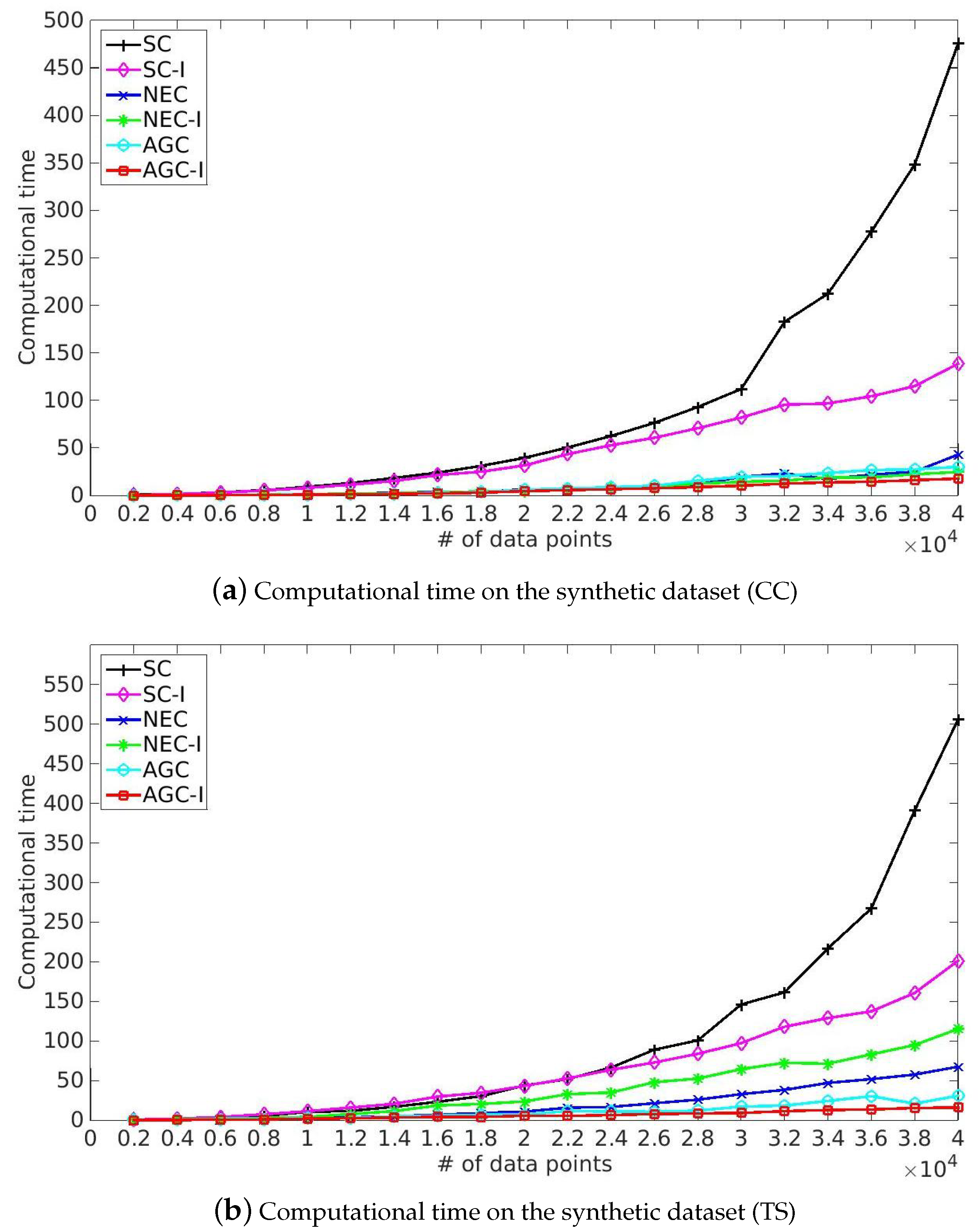
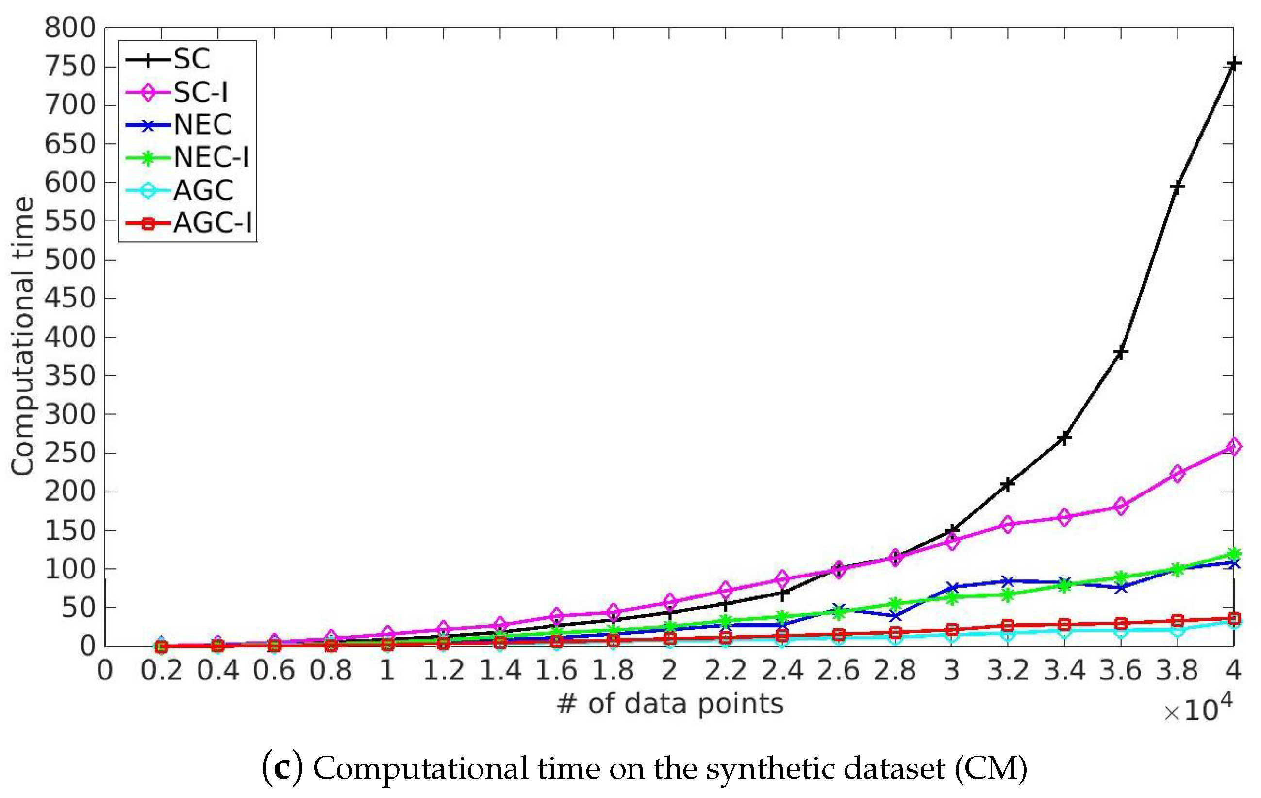
  • SC and the corresponding improved algorithm SC-I achieved competitive performance in term of Purity and NMI. However, SC took more time solving eigenvalue decomposition of Laplacian matrix and our improved algorithm provided a more efficient solution because of the utilization of the multiplicative update optimization. Meanwhile, it took more time to process India Pines because of the rapid growth of time complexity of eigenvalue decomposition of Laplacian matrix caused by the increase of spatial resolution and classes. Note that SC-I, which is based on the multiplicative update algorithm, slightly outperformed SC in terms of Purity and NMI, illustrating that the nonnegative constraint and the orthonormal constraint provided a better indicator matrix. This made it easier to get a robust clustering result by the later processing, such as k-means.
  • NEC and AGC are two efficient improved algorithms and they took only one-twentieth the time in our experiments. Moreover, NEC and AGC could be used on large-scale hyperspectral image datasets such as KSC and Urban, while SC ran out of memory in dealing with the above large-scale datasets because of the storage and time complexity of the affinity matrix. However, the experimental results also illustrate that NEC was not robust enough, which might be because the affinity matrix A can be indefinite and the inverse matrix contains plural elements, making it difficult to get a robust clustering result by k-means. Besides NEC, the other methods did not struggle with this problem, and also provided a better performance than NEC.
  • The proposed NEC-I and AGC-I outperformed the other methods in terms of effectiveness and efficiency. NEC-I and AGC-I firstly take the advantage of sample techniques including Nyström extension and anchor-based graph, which allow them to be used on large-scale hyperspectral image datasets. Furthermore, the proposed multiplicative update algorithm provided an efficient resolution for eigenvalue decomposition of Laplacian matrix. The results presented in Table 5 illustrate that NEC-I and AGC-I performed better than NEC and AGC in most cases. The proposed multiplicative update optimization is flexible and well-knit with the approximated affinity matrix such as Nyström extension and anchor-based graph.

5.5. Computational Time

Figure 3 lists the computational time on three synthetic datasets. We ran the experiments under the same environment: Intel(R) Core(TM) i7-5930K CPU, 3.50 GHz, 64 GB memory, Ubuntu 14.04.5 LTS system and Matlab version R2014b. The methods listed in Figure 3 achieved similar clustering results when there were fewer than 10,000 data points, and SC and SC-I took more time than the other methods when there were more than 10,000 data points. Moreover, the computational time grew rapidly along with the increase of the number of data. The proposed improved algorithm SC-I took only about half the time with more than 30,000 data points. Compared with the above two methods, NEC, AGC and the corresponding improved algorithms NEC-I and AGC-I provided better performance in terms of computational time. Meanwhile, the affinity matrix constructed by the anchor-based graph was better than the affinity matrix constructed by Nyström extension, as the anchor-based graph provided a better way to measure the similarity of data points.

6. Conclusions

In this paper, we briefly review the classical spectral clustering technique for unsupervised HSI classification, and two major problems in dealing with large-scale HSI datasets, namely affinity matrix construction and eigenvalue decomposition of Laplacian matrix. Firstly, we introduce two efficient affinity matrix approximation methods, namely Nyström extension and anchor-based graph, by sampling several HSI pixels. Furthermore, we propose an efficient and effective multiplicative update algorithm to get a robust resolution of eigenvalue decomposition and the experimental results also illustrate that the combination of the affinity matrix approximation and the multiplicative update optimization outperformed the other methods. More importantly, the proposed improved algorithm provides an efficient solution for large-scale HSI classification where the traditional spectral clustering have no capability to deal with them.

Author Contributions

All authors made significant contributions to the manuscript. Y.Z., Y.Y. and Q.W. conceived the research and designed the research framework; Y.Z. designed and implemented the algorithm; and Y.Y. and Q.W. analyzed the results and verified the theory. All authors contributed to the editing of the manuscript.

Funding

This work was supported by the National Natural Science Foundation of China under Grants U1864204 and 61773316; State Key Program of National Natural Science Foundation of China under Grant 61632018; Natural Science Foundation of Shaanxi Province under Grant 2018KJXX-024; Projects of Special Zone for National Defense Science and Technology Innovation; Fundamental Research Funds for the Central Universities under Grant 3102017AX010; and Open Research Fund of Key Laboratory of Spectral Imaging Technology, Chinese Academy of Sciences.

Conflicts of Interest

The authors declare no conflict of interest.

References

  1. Wang, Q.; Wan, J.; Li, X. Robust Hierarchical Deep Learning for Vehicular Management. IEEE Trans. Veh. Technol. 2018. [Google Scholar] [CrossRef]
  2. Wang, Q.; Chen, M.; Nie, F.; Li, X. Detecting Coherent Groups in Crowd Scenes by Multiview Clustering. IEEE Trans. Pattern Anal. Mach. Intell. 2018. [Google Scholar] [CrossRef] [PubMed]
  3. Yan, Q.; Ding, Y.; Xia, Y.; Chong, Y.; Zheng, C. Class probability propagation of supervised information based on sparse subspace clustering for hyperspectral images. Remote Sens. 2017, 9, 1017. [Google Scholar] [CrossRef]
  4. Wang, Q.; Liu, S.; Chanussot, J.; Li, X. Scene classification with recurrent attention of vhr remote sensing images. IEEE Trans. Geosci. Remote Sens. 2018, 57, 1155–1167. [Google Scholar] [CrossRef]
  5. Wang, Q.; He, X.; Li, X. Locality and structure regularized low rank representation for hyperspectral image classification. IEEE Trans. Geosci. Remote Sens. 2018. [Google Scholar] [CrossRef]
  6. He, X.; Wang, Q.; Li, X. Spectral-spatial Hyperspectral image classification via locality and structure constrained low-rank representation. In Proceedings of the IEEE International Geoscience and Remote Sensing Symposium, Valencia, Spain, 23–27 July 2018. [Google Scholar]
  7. Wang, Q.; Meng, Z.; Li, X. Locality adaptive discriminant analysis for spectral-spatial classification of hyperspectral images. IEEE Geosci. Remote Sens. Lett. 2017, 14, 2077–2081. [Google Scholar] [CrossRef]
  8. Yuan, Y.; Lin, J.; Wang, Q. Hyperspectral image classification via multi-task joint sparse representation and stepwise mrf optimization. IEEE Trans. Cybern. 2016, 46, 2966–2977. [Google Scholar] [CrossRef] [PubMed]
  9. Ma, D.; Yuan, Y.; Wang, Q. Hyperspectral anomaly detection via discriminative feature learning with multiple-dictionary sparse representation. Remote Sens. 2018, 10, 745. [Google Scholar] [CrossRef]
  10. Wang, Q.; Zhang, F.; Li, X. Optimal clustering framework for hyperspectral band selection. IEEE Trans. Geosci. Remote Sens. 2018, 56, 5910–5922. [Google Scholar] [CrossRef]
  11. Xie, H.; Zhao, A.; Huang, S.; Han, J.; Liu, S.; Xu, X.; Luo, X.; Pan, H.; Du, Q.; Tong, X. Unsupervised hyperspectral remote sensing image clustering based on adaptive density. IEEE Geosci. Remote Sens. Lett. 2018, 15, 632–636. [Google Scholar] [CrossRef]
  12. Chen, M.; Wang, Q.; Li, X. Discriminant analysis with graph learning for hyperspectral image classification. Remote Sens. 2018, 10, 836. [Google Scholar] [CrossRef]
  13. Fauvel, M.; Benediktsson, J.A.; Chanussot, J.; Sveinsson, J.R. Spectral and spatial classification of hyperspectral data using SVMs and morphological profiles. IEEE Trans. Geosci. Remote Sens. 2008, 46, 3804–3814. [Google Scholar] [CrossRef]
  14. Melgani, F.; Bruzzone, L. Classification of hyperspectral remote sensing images with support vector machines. IEEE Trans. Geosci. Remote Sens. 2004, 42, 1778–1790. [Google Scholar] [CrossRef]
  15. Rodarmel, C.; Shan, J. Principal component analysis for hyperspectral image classification. Surv. Land Inf. Sci. 2002, 62, 115–122. [Google Scholar]
  16. Wang, Q.; Lin, J.; Yuan, Y. Salient band selection for hyperspectral image classification via manifold ranking. IEEE Trans. Neural Netw. Learn. Syst. 2016, 27, 1279–1289. [Google Scholar] [CrossRef] [PubMed]
  17. Wang, Q.; Wan, J.; Nie, F.; Liu, B.; Yan, C.; Li, X. Hierarchical Feature Selection for Random Projection. IEEE Trans. Neural Netw. Learn. Syst. 2018. [Google Scholar] [CrossRef]
  18. Li, J.; Bioucas-Dias, J.M.; Plaza, A. Semisupervised hyperspectral image segmentation using multinomial logistic regression with active learning. IEEE Trans. Geosci. Remote Sens. 2010, 48, 4085–4098. [Google Scholar] [CrossRef]
  19. Chen, Y.; Nasrabadi, N.M.; Tran, T.D. Hyperspectral image classification using dictionary-based sparse representation. IEEE Trans. Geosci. Remote Sens. 2011, 49, 3973–3985. [Google Scholar] [CrossRef]
  20. Chen, Y.; Lin, Z.; Zhao, X.; Wang, G.; Gu, Y. Deep learning-based classification of hyperspectral data. IEEE J. Sel. Top. Appl. Earth Obs. Remote Sens. 2014, 7, 2094–2107. [Google Scholar] [CrossRef]
  21. Zhang, H.; Zhai, H.; Zhang, L.; Li, P. Spectral-spatial sparse subspace clustering for hyperspectral remote sensing images. IEEE Trans. Geosci. Remote Sens. 2016, 54, 3672–3684. [Google Scholar] [CrossRef]
  22. Matasci, G.; Volpi, M.; Kanevski, M.; Bruzzone, L.; Tuia, D. Semisupervised transfer component analysis for domain adaptation in remote sensing image classification. IEEE Trans. Geosci. Remote Sens. 2015, 53, 3550–3564. [Google Scholar] [CrossRef]
  23. Crawford, M.M.; Tuia, D.; Yang, H.L. Active learning: Any value for classification of remotely sensed data? Proc. IEEE 2013, 101, 593–608. [Google Scholar] [CrossRef]
  24. Tuia, D.; Persello, C.; Bruzzone, L. Domain adaptation for the classification of remote sensing data: An overview of recent advances. IEEE Geosci. Remote Sens. Mag. 2016, 4, 41–57. [Google Scholar] [CrossRef]
  25. Guo, X.; Huang, X.; Zhang, L.; Zhang, L.; Plaza, A.; Benediktsson, J.A. Support tensor machines for classification of hyperspectral remote sensing imagery. IEEE Trans. Geosci. Remote Sens. 2016, 54, 3248–3264. [Google Scholar] [CrossRef]
  26. Wang, R.; Nie, F.; Yu, W. Fast spectral clustering with anchor graph for large hyperspectral images. IEEE Geosci. Remote Sens. Lett. 2017, 14, 2003–2007. [Google Scholar] [CrossRef]
  27. Nie, F.; Wang, X.; Jordan, M.I.; Huang, H. The constrained laplacian rank algorithm for graph-based clustering. In Proceedings of the 30th AAAI Conference on Artificial Intelligence, Phoenix, AZ, USA, 12–17 February 2016. [Google Scholar]
  28. Bezdek, J.C. Pattern recognition with fuzzy objective function algorithms. Adv. Appl. Pattern Recognit. 1981, 22, 203–239. [Google Scholar]
  29. Rodriguez, A.; Laio, A. Clustering by fast search and find of density peaks. Science 2014, 344, 1492–1496. [Google Scholar] [CrossRef]
  30. Buckley, J.J. Fuzzy hierarchical analysis. Fuzzy Sets Syst. 1985, 17, 233–247. [Google Scholar] [CrossRef]
  31. Vijendra, S. Efficient clustering for high dimensional data: Subspace based clustering and density based clustering. Inf. Technol. J. 2011, 10, 1092–1105. [Google Scholar] [CrossRef]
  32. Zhong, Y.; Zhang, L.; Gong, W. Unsupervised remote sensing image classification using an artificial immune network. Int. J. Remote Sens. 2011, 32, 5461–5483. [Google Scholar] [CrossRef]
  33. Zhong, Y.; Zhang, S.; Zhang, L. Automatic fuzzy clustering based on adaptive multi-objective differential evolution for remote sensing imagery. IEEE J. Sel. Top. Appl. Earth Obs. Remote Sens. 2013, 6, 2290–2301. [Google Scholar] [CrossRef]
  34. Zhang, L.; You, J. A spectral clustering based method for hyperspectral urban image. In Proceedings of the 2017 Joint Urban Remote Sensing Event (JURSE), Dubai, UAE, 6–8 March 2017; pp. 1–3. [Google Scholar]
  35. Zhao, Y.; Yuan, Y.; Nie, F.; Wang, Q. Spectral clustering based on iterative optimization for large-scale and high-dimensional data. Neurocomputing 2018, 318, 227–235. [Google Scholar] [CrossRef]
  36. Bai, J.; Xiang, S.; Pan, C. A graph-based classification method for hyperspectral images. IEEE Trans. Geosci. Remote Sens. 2013, 51, 803–817. [Google Scholar] [CrossRef]
  37. Camps-Valls, G.; Marsheva, T.V.B.; Zhou, D. Semi-supervised graph-based hyperspectral image classification. IEEE Trans. Geosci. Remote Sens. 2007, 45, 3044–3054. [Google Scholar] [CrossRef]
  38. Wang, Q.; Qin, Z.; Nie, F.; Li, X. Spectral Embedded Adaptive Neighbors Clustering. IEEE Trans. Neural Netw. Learn. Syst. 2018. [Google Scholar] [CrossRef] [PubMed]
  39. Belongie, S.; Fowlkes, C.; Chung, F.; Malik, J. Spectral partitioning with indefinite kernels using the Nyström extension. In Proceedings of the European Conference on Computer Vision, Copenhagen, Denmark, 28–31 May 2002; pp. 531–542. [Google Scholar]
  40. Fowlkes, C.; Belongie, S.; Chung, F.; Malik, J. Spectral grouping using the Nystrom method. IEEE Trans. Pattern Anal. Mach. Intell. 2004, 26, 214–225. [Google Scholar] [CrossRef]
  41. Tang, X.; Jiao, L.; Emery, W.J.; Liu, F.; Zhang, D. Two-stage reranking for remote sensing image retrieval. IEEE Trans. Geosci. Remote Sens. 2017, 55, 5798–5817. [Google Scholar] [CrossRef]
  42. Zhang, X.; Jiao, L.; Liu, F.; Bo, L.; Gong, M. Spectral clustering ensemble applied to sar image segmentation. IEEE Trans. Geosci. Remote Sens. 2008, 46, 2126–2136. [Google Scholar] [CrossRef]
  43. Zhu, W.; Nie, F.; Li, X. Fast Spectral Clustering with efficient large graph construction. In Proceedings of the IEEE International Conference on Speech and Signal Processing, New Orleans, LA, USA, 5–9 March 2017; pp. 2492–2496. [Google Scholar]
  44. Nie, F.; Zhu, W.; Li, X. Unsupervised Large Graph Embedding. In Proceedings of the 31st AAAI Conference on Artificial Intelligence, San Francisco, CA, USA, 4–9 February 2017; pp. 2422–2428. [Google Scholar]
  45. Yokoya, N.; Yairi, T.; Iwasaki, A. Coupled nonnegative matrix factorization unmixing for hyperspectral and multispectral data fusion. IEEE Trans. Geosci. Remote Sens. 2012, 50, 528–537. [Google Scholar] [CrossRef]
  46. Jia, S.; Qian, Y. Constrained nonnegative matrix factorization for hyperspectral unmixing. IEEE Trans. Geosci. Remote Sens. 2009, 47, 161–173. [Google Scholar] [CrossRef]
  47. Shi, J.; Malik, J. Normalized cuts and image segmentation. IEEE Trans. Pattern Anal. Mach. Intell. 2000, 22, 888–905. [Google Scholar]
  48. Nie, F.; Ding, C.; Luo, D.; Huang, H. Improved minmax cut graph clustering with nonnegative relaxation. In Proceedings of the Joint European Conference on Machine Learning and Knowledge Discovery in Databases, Barcelona, Spain, 20–24 September 2010; pp. 451–466. [Google Scholar]
  49. Türkmen, A.C. A review of nonnegative matrix factorization methods for clustering. Comput. Sci. 2015, 1, 405–408. [Google Scholar]
  50. Fowlkes, C.; Belongie, S.; Malik, J. Efficient spatiotemporal grouping using the Nyström method. In Proceedings of the IEEE Computer Society Conference on Computer Vision and Pattern Recognition, Kauai, HI, USA, 8–14 December 2001. [Google Scholar]
  51. Liu, W.; He, J.; Chang, S.F. Large Graph Construction for Scalable Semi-Supervised Learning. In Proceedings of the 27th International Conference on Machine Learning, Haifa, Israel, 22–24 June 2010. [Google Scholar]
Figure 1. The synthetic datasets.
Remotesensing 11 00399 g001
Figure 2. HSI ground truth and results.
Remotesensing 11 00399 g002
Figure 3. Computational time on three synthetic datasets.
Remotesensing 11 00399 g003aRemotesensing 11 00399 g003b
Table 1. Notation.
Table 1. Notation.
WAffinity (or similarity) matrix
D Diagonal matrix
L Laplacian matrix
Y Cluster indicator matrix
y Cluster indicator
x Pixels (or data points)
I Identity matrix
nNumber of pixels
mNumber of chosen pixels (or anchors)
dNumber of spectral bands
cNumber of classes
Table 2. Clustering results on synthetic dataset (CC).
SCSC-INECNEC-IAGCAGC-I
P.NMICTP.NMICTP.NMICTP.NMICTP.NMICTP.NMICT
Num. = 20001.001.001.021.001.000.350.680.250.051.001.000.081.001.000.051.001.000.06
Num. = 40001.001.001.451.001.001.350.650.090.141.001.000.171.001.000.151.001.000.14
Num. = 60001.001.003.121.001.002.940.690.260.361.001.000.481.001.000.261.001.000.29
Num. = 80001.001.005.531.001.005.230.670.250.681.001.000.811.001.000.561.001.000.54
Num. = 10,0001.001.009.051.001.007.870.680.250.811.001.001.251.001.000.691.001.000.86
Num. = 12,0001.001.0013.041.001.0011.350.500.001.911.001.001.891.001.000.831.001.001.20
Num. = 14,0001.001.0018.391.001.0015.230.570.022.671.001.002.321.001.001.131.001.001.62
Num. = 16,0001.001.0023.991.001.0021.440.520.003.661.001.003.011.001.001.331.001.002.17
Num. = 18,0001.001.0031.051.001.0025.000.630.193.251.001.004.421.001.001.851.001.002.87
Num. = 20,0001.001.0039.521.001.0031.520.690.276.591.001.004.551.001.002.231.001.004.58
Num. = 22,0001.001.0050.361.001.0043.480.500.005.581.001.007.191.001.003.061.001.005.57
Num. = 24,0001.001.0062.551.001.0052.810.540.007.131.001.008.401.001.003.791.001.006.54
Num. = 26,0001.001.0076.381.001.0060.660.530.009.171.001.008.881.001.004.541.001.007.57
Num. = 28,0001.001.0093.061.001.0070.780.690.2611.591.001.0012.340.830.475.451.001.008.78
Num. = 30,0001.001.00111.981.001.0081.950.740.2819.521.001.0014.341.001.008.121.001.0010.31
Num. = 32,0001.001.00182.781.001.0095.470.590.1523.141.001.0015.630.830.4810.011.001.0012.43
Num. = 34,0001.001.00212.341.001.0096.860.630.2017.351.001.0018.901.001.0010.301.001.0013.72
Num. = 36,0001.001.00277.531.001.00104.320.510.0021.861.001.0019.131.001.0031.711.001.0014.41
Num. = 38,0001.001.00348.301.001.00115.030.500.0024.991.001.0022.331.001.0023.171.001.0016.07
Num. = 40,0001.001.00475.561.001.00138.640.570.1243.011.001.0024.661.001.0018.091.001.0017.70
Average1.001.00101.851.001.0049.110.600.1310.171.001.008.540.980.956.371.001.006.37
Table 3. Clustering results on synthetic dataset (TS).
SCSC-INECNEC-IAGCAGC-I
P.NMICTP.NMICTP.NMICTP.NMICTP.NMICTP.NMICT
Num. = 20000.970.831.011.000.980.500.500.010.080.990.930.171.001.000.820.950.710.14
Num. = 40000.980.851.400.980.881.920.730.220.381.000.960.871.001.000.400.980.870.24
Num. = 60000.970.832.950.970.823.980.500.000.681.000.981.761.001.000.870.990.930.43
Num. = 80000.970.795.410.990.937.400.500.001.260.990.942.631.001.001.041.000.960.97
Num. = 10,0000.970.818.370.990.9511.270.500.002.351.000.954.091.001.002.680.870.451.90
Num. = 12,0000.970.7913.390.990.9415.810.500.003.460.990.957.651.001.002.750.950.712.41
Num. = 14,0000.970.7918.700.980.8920.610.710.295.010.990.9111.431.001.004.770.980.873.31
Num. = 16,0000.970.7926.490.830.3529.710.510.036.790.960.8018.551.001.005.680.990.934.14
Num. = 18,0000.970.8132.980.990.9234.420.680.258.970.990.9520.361.001.006.821.000.964.03
Num. = 20,0000.970.8243.030.990.9043.230.500.0010.820.990.9323.611.001.006.960.920.595.59
Num. = 22,0000.970.7955.620.990.9352.660.720.3015.710.990.9432.811.001.0011.390.950.715.30
Num. = 24,0000.970.8072.020.990.9563.610.520.0116.680.990.9334.861.001.0010.940.980.876.48
Num. = 26,0000.970.8085.320.990.9472.830.530.0321.370.990.9148.001.001.0010.660.990.937.71
Num. = 28,0000.970.80102.270.990.9583.750.500.0025.860.990.9552.511.001.0011.991.000.968.52
Num. = 30,0000.970.81149.991.000.9897.310.510.0332.830.990.9464.451.001.0017.101.001.009.06
Num. = 32,0000.970.81190.720.990.93118.010.500.0038.240.990.9472.441.001.0018.381.000.9811.40
Num. = 34,0000.970.81258.660.980.88128.900.510.0347.000.990.9571.321.001.0024.320.910.5712.86
Num. = 36,0000.970.81358.370.980.86137.450.500.0051.820.990.9483.111.001.0030.240.980.8913.48
Num. = 38,0000.970.80459.320.970.82160.640.500.0057.570.680.1094.871.001.0020.890.980.0415.44
Num. = 40,0000.970.81636.230.990.94201.300.500.0067.461.000.97115.241.001.0030.731.001.0015.88
Average0.970.81126.310.980.8964.270.550.0620.720.980.8938.041.001.0010.970.970.806.46
Table 4. Clustering results on synthetic dataset (CM).
SCSC-INECNEC-IAGCAGC-I
P.NMICTP.NMICTP.NMICTP.NMICTP.NMICTP.NMICT
Num. = 20001.001.000.381.000.980.700.500.000.091.001.000.170.560.190.861.001.000.08
Num. = 40001.001.001.340.990.922.430.500.001.501.001.000.851.001.000.411.001.000.29
Num. = 60001.001.002.700.990.905.220.500.001.081.001.001.631.001.001.141.001.000.81
Num. = 80001.001.005.710.990.919.640.890.531.901.001.003.221.001.002.131.001.001.48
Num. = 10,0001.001.008.460.990.9515.390.500.003.051.001.005.321.001.002.201.001.002.34
Num. = 12,0001.001.0012.550.990.9521.760.500.014.701.001.008.241.001.003.731.001.003.42
Num. = 14,0001.001.0018.240.990.9427.110.500.008.471.001.0012.491.001.003.741.001.004.64
Num. = 16,0001.001.0026.760.930.6339.330.500.0010.851.001.0017.261.001.004.501.001.006.28
Num. = 18,0001.001.0034.210.990.9244.150.900.5515.681.001.0020.801.001.006.511.001.007.63
Num. = 20,0001.001.0043.860.990.9257.080.500.0021.381.001.0025.601.001.007.781.001.009.60
Num. = 22,0001.001.0055.550.990.9472.230.500.0027.261.001.0033.161.001.008.481.001.0011.20
Num. = 24,0001.001.0069.450.990.9586.580.680.2527.871.001.0038.491.001.008.981.001.0013.34
Num. = 26,0001.001.00101.070.990.9599.360.500.0148.771.001.0044.621.001.0011.411.001.0015.60
Num. = 28,0001.001.00114.920.990.95114.370.500.0039.561.001.0055.301.001.0011.831.001.0017.92
Num. = 30,0001.001.00149.531.000.96136.300.910.5976.801.001.0063.811.001.0014.981.001.0021.26
Num. = 32,0001.001.00209.870.990.93158.110.850.4984.711.001.0067.091.001.0016.841.001.0027.18
Num. = 34,0001.001.00270.500.990.91167.200.500.0082.731.001.0079.641.001.0020.621.001.0028.29
Num. = 36,0001.001.00381.080.990.91181.040.620.0476.131.001.0089.441.001.0020.621.001.0030.00
Num. = 38,0001.001.00594.830.960.75223.330.770.3799.991.001.00100.111.001.0021.471.001.0033.28
Num. = 40,0001.001.00754.120.990.93258.650.500.00108.561.001.00119.931.001.0032.861.001.0036.46
Average1.001.00142.760.990.9186.000.610.1437.051.001.0039.360.980.9610.051.001.0013.55
Table 5. Clustering results on hyperspectral image datasets. The bold numbers represent the best results in terms of purity, normalization of the mutual information and computational time.
SCSC-INECNEC-IAGCAGC-I
PUI.NMICTPUI.NMICTPUI.NMICTPUI.NMICTPUI.NMICTPUI.NMICT
Samson0.850.616.570.850.605.770.730.530.100.850.600.170.880.730.190.910.750.19
Jasper0.830.7110.310.910.766.430.700.560.030.830.710.110.720.660.090.820.700.14
SalinasA0.810.804.770.850.794.310.780.770.060.800.810.170.790.780.100.840.810.15
India Pines0.360.4466.210.460.4645.370.430.450.530.430.491.290.350.430.580.420.461.46
Salinas------0.600.721.620.620.714.620.560.672.440.560.713.55
Pavia Uni.------0.470.341.340.610.573.340.460.513.400.540.573.67
KSC------0.460.571.160.510.525.970.470.526.100.510.536.48
Urban------0.400.120.410.450.213.010.510.331.140.500.293.12
Average0.680.5827.690.740.6019.190.570.510.660.640.582.340.590.581.760.640.602.35

