Article

Spatiotemporal Variability of Remote Sensing Ocean Net Primary Production and Major Forcing Factors in the Tropical Eastern Indian and Western Pacific Ocean

1
Key Laboratory of Digital Earth Science, Institute of Remote Sensing and Digital Earth, Chinese Academy of Sciences, Beijing 100094, China
2
University of Chinese Academy of Sciences, Beijing 100049, China
*
Author to whom correspondence should be addressed.
Remote Sens. 2019, 11(4), 391; https://doi.org/10.3390/rs11040391
Submission received: 29 December 2018 / Revised: 1 February 2019 / Accepted: 12 February 2019 / Published: 15 February 2019
(This article belongs to the Special Issue Remote Sensing of Ocean Primary Production)

Abstract

:
Based on widely used remote sensing ocean net primary production (NPP) datasets, the spatiotemporal variability of NPP is first analyzed over the tropical eastern Indian and western Pacific Ocean for the period 1998–2016 using the conventional empirical orthogonal function (EOF), the lead–lag correlation and the ensemble empirical mode decomposition (EEMD) technique. Barnett and Preisendorfer’s improved Canonical Correlation Analysis (BPCCA) is also applied to derive covariability patterns of NPP with major forcing factors of the chlorophyll a concentration (Chla), sea surface temperature (SST), sea level anomaly (SLA), ocean rainfall (Rain), sea surface wind (Wind), and current (CUR) under climate changes of El Niño–Southern Oscillation (ENSO) and Indian Ocean Dipole (IOD). We find that: (1) The first two seasonal EOF modes capture significant temporal and meridional NPP variability differences, as NPP reaches peaks approximately three months later in the western Pacific Ocean than that of in the eastern Indian Ocean. (2) The second and third interannual EOF modes are closely related with ENSO with a two-month lag and synchronous with IOD, respectively, characterized by southwesterly positive anomaly centers during positive IOD years. (3) NPP presents different varying tendencies and similar multiscale oscillation patterns with interannual and interdecadal cycles of 2~3 years, 5~8 years, and 9~19 years in subregions of the Bay of Bengal, the South China Sea, the southeastern Indian Ocean, and the northwestern Pacific Ocean. (4) The NPP variability is strongly coupled with negative SST, SLA, and Rain anomalies, as well as positive Chla, Wind and CUR anomalies in general during El Niño/positive IOD years. The results reveal the diversity and complexity of large-scale biophysical interactions in the key Indo-Pacific Warm Pool region, which improves our understanding of ocean productivity, ecosystems, and carbon budgets.

Graphical Abstract

1. Introduction

Contributing roughly half of the biosphere’s net primary production (NPP), photosynthesis by oceanic phytoplankton is a vital link in the cycling of carbon between living and inorganic stocks, whose variability profoundly affects the global carbon cycle and climate changes [1,2]. As ocean absorption of atmospheric CO2 can contribute to moderate future climate change and the marine environment. Moreover, additional large-scale modifications associated to global change such as the predicted alterations in ocean chemistry, temperature, and so on are also expected to impact considerably marine ecosystems. Therefore, the distribution and dynamic variability of ocean NPP and its relationship with physical driving factors and climate indices have received increasing attention with the accumulation of multiple remote sensing products over the past decades [3,4,5,6].
Compared to the seas off Somalia and the Arabian Sea, few studies have focused on the biological variability associated with ocean physical environments in the tropical eastern Indian Ocean [7,8,9,10,11,12,13,14]. In addition, existing studies mainly investigate the strongly impacted chlorophyll a concentration (Chla) off the coast of Java by monsoon-driven currents and upwelling changes on a seasonal timescale or interannual modulation driven by the Indian Ocean Dipole (IOD). El Niño–Southern Oscillation (ENSO), as a well-known interannual climate mode, develops in the tropical Pacific. Its remote forcing on biological variation in the tropical eastern Indian Ocean has received far less attention, with the exception of Currie et al. [7], who studied the Chla anomaly patterns for the period 1961–2001 driven by ENSO and IOD within the Indian Ocean using a coupled model. Meanwhile, many studies have committed to the biological variability in the tropical western Pacific Ocean. The ocean primary production has been found to be low in the western Pacific but with strong biological variability associated with ENSO [15,16,17,18,19]. Though the spatiotemporal variability of Chla associated with the physical variables of sea surface temperature (SST), sea level anomaly (SLA), sea surface wind (Wind) and ENSO have been studied in western Pacific on seasonal and interannual timescale by Hou et al. [17], the possible influence of IOD events was not included.
The tropical eastern Indian and western Pacific Ocean between 25°S–25°N and 75°–165°E (Figure 1) is known as a key Indo-Pacific Warm Pool region, which is characterized by low surface salinity and oligotrophic conditions but is sensitive to climate changes. The Indonesian Throughflow (ITF) here allows low latitude exchanges between the western Pacific and eastern Indian Ocean, which impacts the basin-scale biogeochemistry of the eastern Indian Ocean [20]. However, spatiotemporal biophysical variability patterns and their responses to two climate modes of ENSO and IOD in the study area have not been available to date. Therefore, we systematically analyze the seasonal to interannual variability and long-term trends of NPP as well as the covariability patterns with typical environmental variables (Chla, SST, SLA, Rain, Wind, and Current) over the tropical eastern Indian and western Pacific Ocean during 1998–2016, using the conventional empirical orthogonal function (EOF) analysis, the lead–lag correlation analysis, the ensemble empirical mode decomposition (EEMD) analysis and the Barnett and Preisendorfer improved Canonical Correlation Analysis (BPCCA).
The paper is organized as follows. Section 2 describes the various datasets and methods used. The results in Section 3 include the following four parts: (1) dominant seasonal NPP variability patterns through the EOF analysis; (2) dominant interannual NPP variability through the EOF and the lead–lag correlation analysis; (3) long-term trends and multiscale oscillation patterns of NPP through the EEMD analysis in four subregions of the Bay of Bengal (BoB), the South China Sea (SCS), the southeastern Indian Ocean and the northwestern Pacific Ocean; and (4) covariability patterns of NPP with major forcing factors on an interannual timescale through the BPCCA analysis. Finally, the discussion and conclusions are provided in Section 4 and Section 5.

2. Datasets and Methods

2.1. Datasets

The multisource satellite observation and reanalysis products from January 1998 to December 2016 are obtained. NPP datasets are from the Standard VGPM algorithm based on SeaWiFS and MODIS from the Ocean Productivity site. The VGPM is a ‘chlorophyll-based’ model that estimates net primary production from chlorophyll using a temperature-dependent description of chlorophyll-specific photosynthetic efficiency [21]. Though studies have suggested that VGPM predicts larger NPP in temperate and subpolar regions and lower values in equatorial regions compare to Eppley-VGPM, it still keeps the robust nature of the primary temporal trends of the NPP [1,22,23,24]. The VGPM NPP does provide a means of quantifying ocean productivity on a regional or global scale and linking its variability to environmental factors. We also use Chla datasets from the Ocean Color Climate Change Initiative (OC-CCI); SST datasets from the NOAA High Resolution SST data provided by the NOAA/OAR/ESRL PSD; SLA datasets from the Archiving, Validation and Interpretation of Satellite Oceanographic (AVISO); rain datasets from the Tropical Rainfall Measuring Mission (TRMM) 3B43 precipitation product, provided by the NASA Goddard Earth Sciences Data and Information Services Center (GES DISC); wind datasets from the Cross-Calibrated Multi-Platform (CCMP) Version-2.0 vector wind analyses produced by Remote Sensing Systems; and ocean current (CUR) datasets from the GLOBAL-REANALYSIS-PHY-001-030 reanalysis product provided by the Copernicus Marine Environment Monitoring Service (CMEMS). Variables and their sources, timespans, and temporal–spatial resolutions are described in Table 1.
In addition, two climate variability indices are used, the representative multivariate ENSO index (MEI) and dipole mode index (DMI), whose positive values can characterize El Niño/positive IOD years (IODs) while negative values represent La Niña/negative IODs.

2.2. Data Preprocessing

To get monthly mean NPP datasets, we multiplied each pixel by the number of days represented by the downloaded files (monthly) to transform units of mg C/m2/day to mg C/m2/month. Before proceeding with any long time series analysis, all variables were resampled to grids of 0.25° by 0.25° for computational efficiency. Since the computation of EOF analysis required no gaps in the time series, the missing values were filled by interpolating spatially adjacent values, if they existed. Pixels where the original time series contained more than 50% missing data were set as NAN, and the remaining gaps were filled at each pixel using a temporal linear interpolation. In particular, due to the approximated lognormal distribution of satellite-derived NPP and Chla, they were log-transformed before the EOF analysis [17,25]. We also removed seasonal cycles to get standardized monthly mean anomaly fields of variables using the z-score algorithm, which calculates the mean and standard deviation for a given month’s values, and then standardizes each value by subtracting the mean and dividing by the standard deviation [26].

2.3. Methods

The empirical orthogonal function (EOF) analysis was used on the climatological monthly mean NPP fields over the 19 years and standardized monthly NPP anomaly fields, respectively, to study the seasonal and interannual variability of NPP. EOF is a statistical method for diagonalizing the covariance matrix of a given field into a set of eigenvalues and corresponding eigenvectors and then projecting the eigenvectors onto the original field to obtain a time series [27]. Thus, the variability of the field is decomposed into sums of modes, each of which is described by a spatial pattern (the so-called EOF) and a time series (principal component, PC) [28]. The statistical significance test of the EOF modes is based on the rule of thumb proposed by North et al. [29]. Furthermore, the lead–lag correlation analysis was used to estimate the time lags of the NPP variability associated with the climate modes of ENSO and IOD.
The traditional linear regression analysis has been widely used to assess the trend of ocean chlorophyll and productivity [1,4,30]. However, to identify more complex variations of NPP, we used the ensemble empirical mode decomposition (EEMD) technique designed for adaptive analysis of nonlinear and nonstationary time series [31], which has been recently applied to characterize significant Chla oscillation patterns and trend estimation [32,33].The statistical significance of IMFs is based on the distribution of energy as a function of the mean period of the IMF relative to that of pure white noise. This method allows one to differentiate true signals from components of noise with any selected statistical significance level (90%, 95%, or 99%).
To identify coupling patterns of NPP with typical physical variables, we chose the improved canonical correlation analysis presented by Barnett and Preisendorfer [34], namely BPCCA. The resulting coupled modes aim to successively maximize the covariability between the given pair of fields [35]. The BPCCA is followed to filter out small-scale noise in the datasets and to produce more stable patterns than the classical CCA, which is particularly apparent when the sample size is smaller than the spatial dimensionality of the field. Accordingly, on the basis of the EOF analysis, only the most relevant orthogonal modes (cumulatively representing approximately 70% of the temporal variance) are retained for the CCA [36]. The Bartlett–Lawley significance test is applied at the 95% confidence level in order to assess the statistical significance of the couple modes [37].

3. Results and Analysis

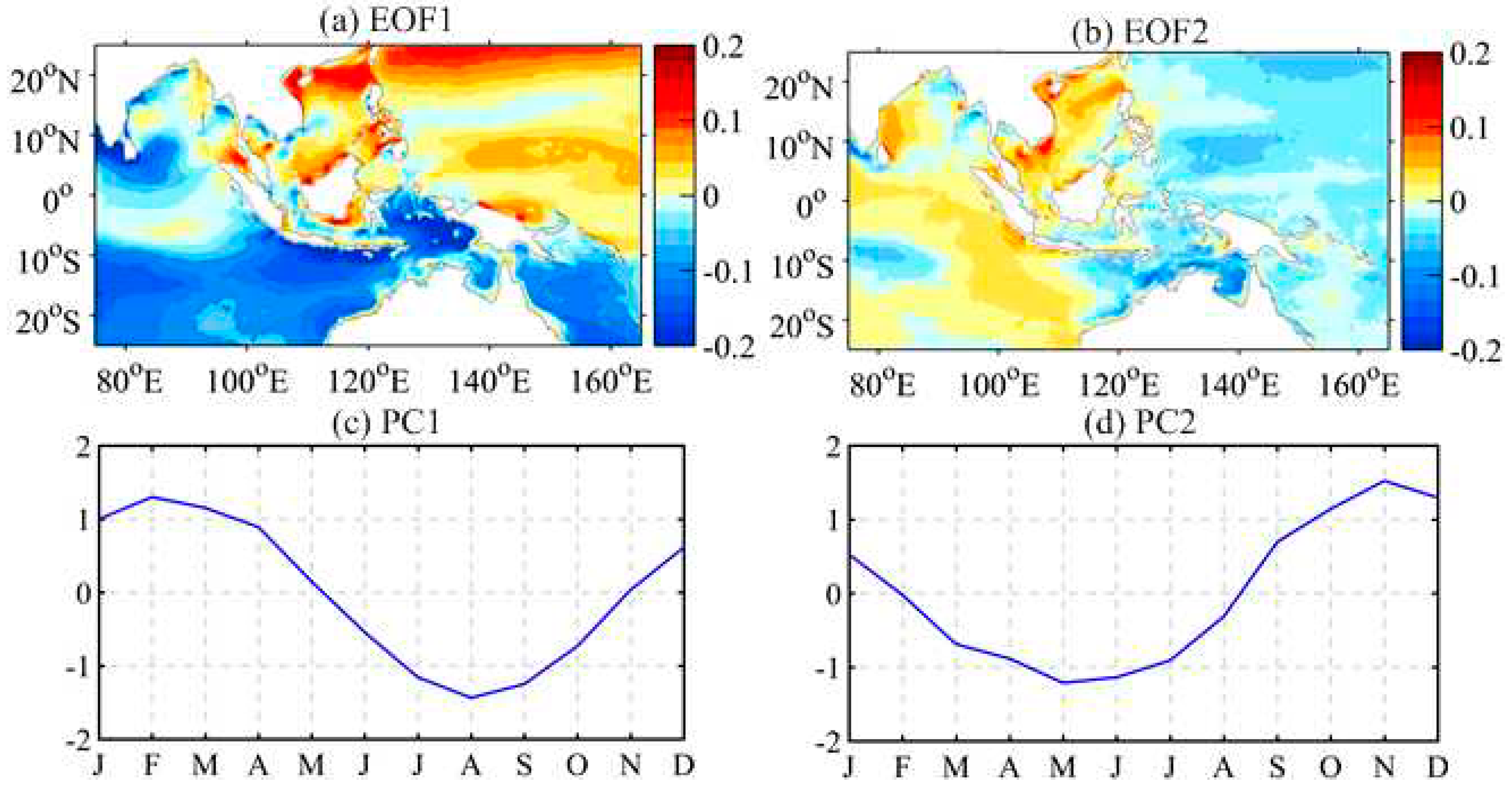
3.1. Dominant Seasonal NPP Variability Patterns

For the EOF on monthly mean NPP fields, the first two modes, which accounts for 71.71% and 11.85% of the total variance, respectively, capture the dominant seasonal variability patterns. The spatial patterns and their corresponding principal components are shown in Figure 2. The positive (negative) spatial distributions and positive (negative) temporal coefficients yield positive NPP anomalies, whereas the positive (negative) spatial distributions and negative (positive) temporal coefficients yield negative NPP anomalies.
In terms of the temporal variation, the first principal component (PC1) shown in Figure 2c indicates the seasonal NPP variation, with peaks in boreal winter (January–February) and troughs in boreal summer (July–August), whereas PC2 shown in Figure 2d exhibits variation with peaks in boreal autumn (October–November) and troughs in boreal spring (April–May). The combination of the two modes thus describes a consecutive annual cycle of NPP variations over the study area.
Figure 2a shows the NPP variation pattern in boreal winter and summer, with an approximate southwest–northeast trend but opposite structure. Specifically, for boreal winter, significant positive anomalies exist in most of the western Pacific region, which means that NPP remarkably increases in the SCS, the north Pacific subtropical oligotrophic region and seas north of New Guinea, as well as the northeastern BoB. Meanwhile, NPP shows an obvious reduction during boreal winter in almost all the eastern Indian Ocean, especially in seas around Sri Lanka and south of 10°S in the southeastern Indian Ocean, as well as the Java-Banda Sea and seas of northeastern Australia in the western Pacific. In addition, the reverse situation occurs in boreal summer.
Figure 2d presents the transition variation pattern of NPP in boreal autumn and spring. The boreal autumn positive maxima describe weak late summer peaks in the western BoB, the equatorial Indian Ocean, the coasts of Sumatra and Java and the entire SCS basin. Meanwhile, NPP decreases in most of the western Pacific, the eastern Seychelles–Chagos Thermocline Ridge (SCTR) along 10°S and the northern coast of Australia in boreal autumn. In contrast, the reverse situation occurs in boreal spring. Briefly, the first two EOF modes capture the significant temporal and meridional NPP variability differences in the study area, as NPP reaches peaks approximately three months later in the western Pacific than that of in the eastern Indian Ocean.

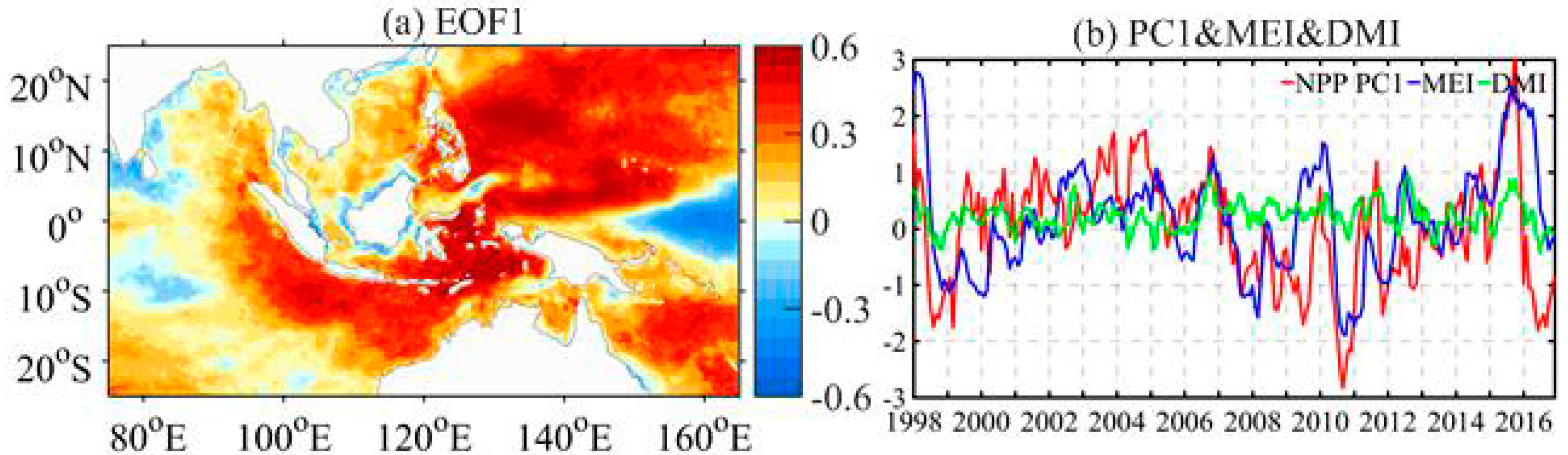
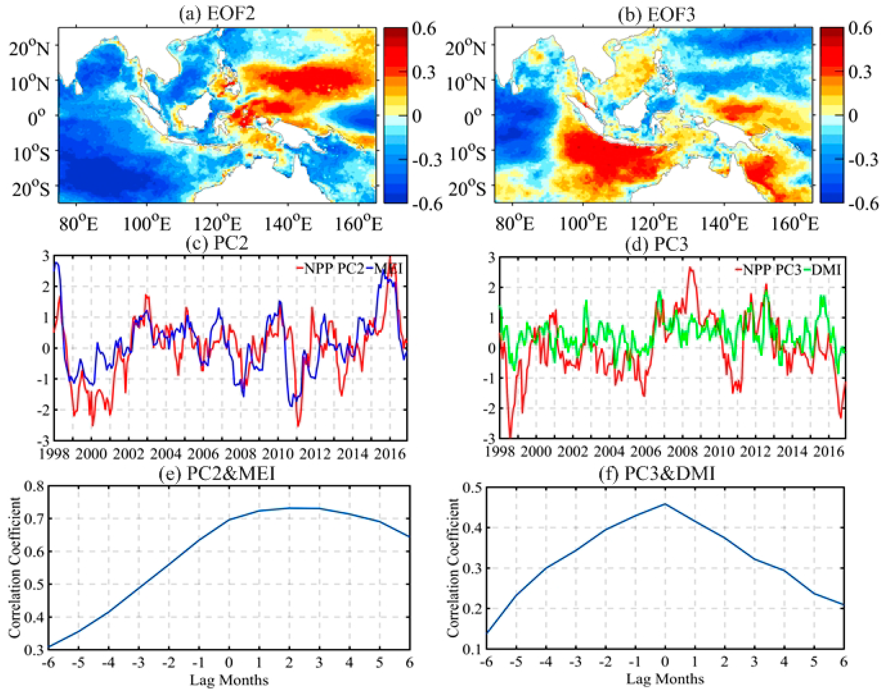
3.2. Dominant Interannual NPP Variability Patterns

The interannual NPP variability is determined using the EOF on standardized monthly mean anomaly fields. The first three leading modes accounting for 9.43%, 8.61%, and 5.03% of the total variance, respectively, and all passed the statistical significant test at the 95% confidence level. Correlations of the first three principal components with MEI and DMI are listed in Table 2. The first mode is found to be associated with MEI and DMI, with correlations of 0.46 and 0.23, respectively, which indicates the combined action of ENSO and IOD. However, here we only focus on the second and third modes, which are strongly correlated with MEI and DMI separately. The spatial distribution and principal components of these three modes are shown in Figure 3 and Figure 4.
The time series of PC2 and MEI are highly correlated with a correlation coefficient of 0.65 and a two-month time lag (Figure 4c,e), which indicates that the second EOF mode captures the interannual NPP variability associated with ENSO. The positive PC2 values plotted in Figure 4c coincide with El Niño years, namely, 2002–2003, 2004–2005, 2006–2007, 2009–2010, and 2014–2016, and negative values coincide with La Niña years, namely, 1998–2000, 2000–2001, 2007–2008, 2010–2011, and 2011–2012. The spatial pattern of EOF2 shown in Figure 4a is characterized by a negative–positive dipole structure with one conspicuous positive anomaly center located in the eastern Philippines and northern New Guinea seas during El Niño years. The strongest negative anomalies are found in the southern SCS, the equatorial Pacific east of 155°E, as well as the western BoB and central southern Indian Ocean during El Niño years. The reverse NPP anomalies occur over similar regions during La Niña events.
The time series of PC3 has no close relationship with MEI (the correlation coefficient is 0.05) but is obviously correlated with DMI, with a correlation coefficient of 0.48 and no time lag (Figure 4d,f), which means that the third EOF mode describes an IOD-associated pattern. Moreover, the positive values of PC3 coincide with positive IODs of 2006, 2007, 2008, 2011, 2012, and 2015, and negative values coincide with negative IODs of 1998, 2005, 2010, 2013, and 2016. The spatial pattern of EOF3 presents an obvious negative–positive–negative anomaly feature, with positive anomalies existing in the deep basin of SCS and around the Indonesian archipelago, including coasts of Sumatra and Java, the Banda Sea, and the northeastern coasts of New Guinea and Australia during positive IODs (Figure 4b). Meanwhile, negative NPP anomalies are mainly found in the seas south of India, the Sulu Sea, and the north Pacific subtropical oligotrophic region. During negative IODs, the opposite NPP anomalies can be discovered over similar regions.
It is noteworthy that the increased NPP off the coasts of Sumatra and Java is caused by IOD and ENSO, though the variability explained by IOD is far greater than that of ENSO (Figure 4a,b). In the central southern Indian Ocean and southern SCS, marked converse variability is discovered, with increased NPP induced by positive IODs and decreased NPP related to El Niño. Particularly notable is that significant positive NPP anomalies induced by positive IODs are found first off the coasts of New Guinea and the Solomon Islands.

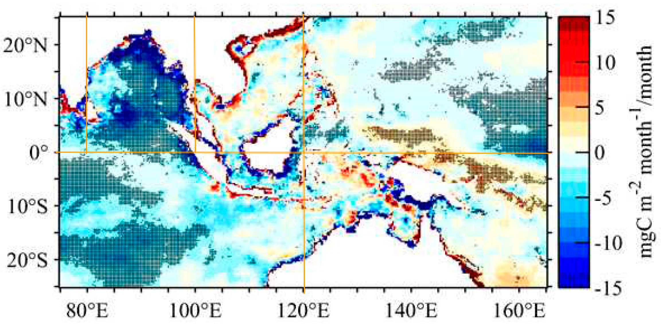
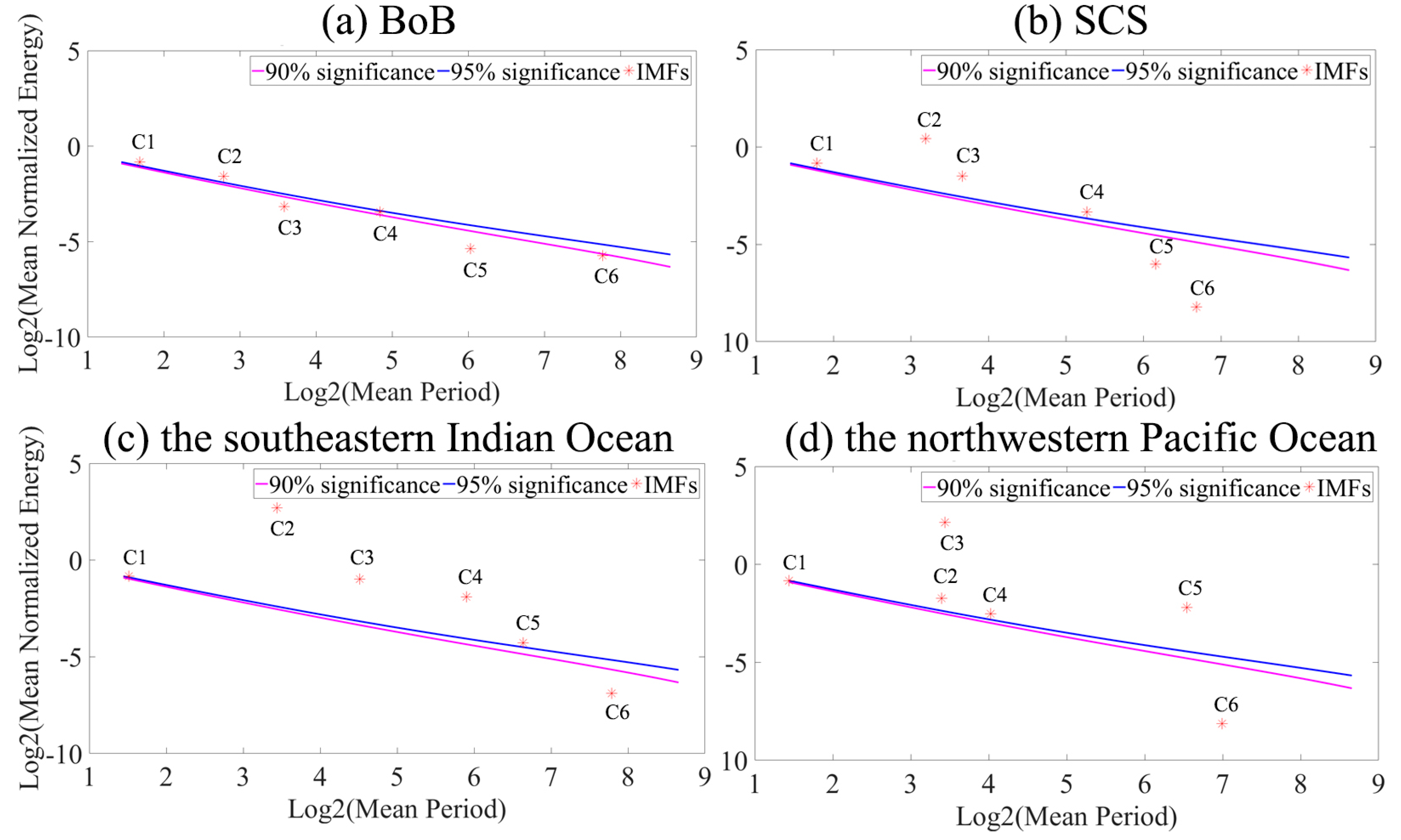
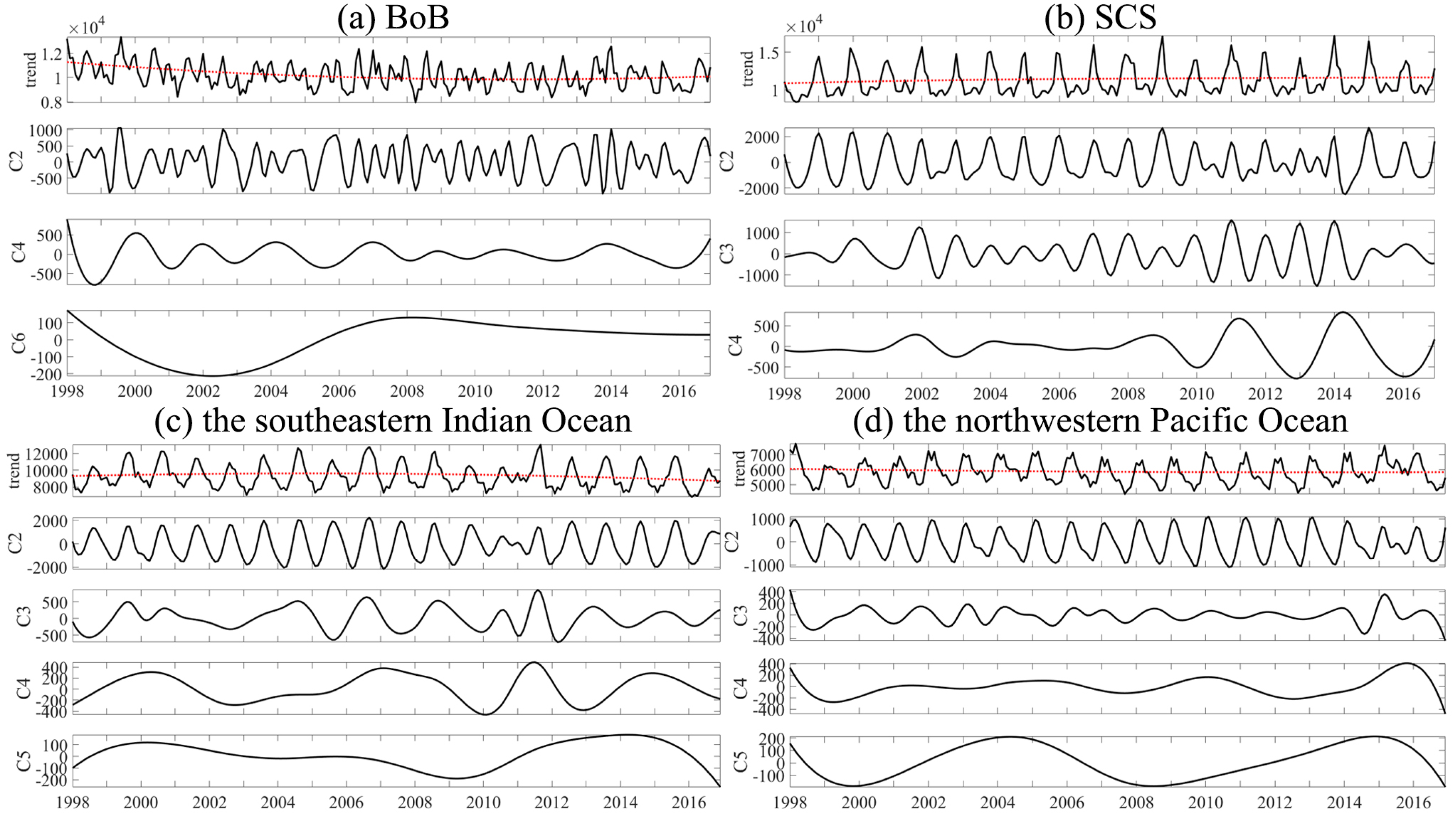
3.3. Long-Term Trend and Multiscale Oscillation Patterns of NPP

To identify more complex variations of NPP in the study area, first, we calculate NPP trends on a point-by-point basis using the linear regression analysis to understand changes occurring over the past 19 years intuitively. The trend distribution map is shown in Figure 5.
Negative trends are apparent in the study area, particularly on the northeastern coasts and southern BoB, as well as open seas south of India and the north subtropical and equatorial Pacific (Figure 5). There are also significant positive trends along the northwestern coasts of SCS and seas of northeastern New Guinea and the Solomon Islands, while weaker increases are also distributed in the southern SCS, northeastern Banda Sea and eastern seas of Australia. Then, we divide four subregions to compare the multi-timescale variability of NPP in detail, namely, the Bay of Bengal (BoB, 80°–100°E, 0°–25°N), the South China Sea (SCS, 100°–120°E, 0°–25°N), the southeastern Indian Ocean (75°–120°E, 0°–25°S), and northwestern Pacific Ocean (120°–165°E, 0°–25°N).
Using the EEMD analysis for NPP in these four subregions, the significant tests of IMFs are shown in Figure 6 with respect to their mean period and corresponding energy. The statistically significant IMFs and residual components are shown in Figure 7, with their corresponding mean periods and variance contribution rates shown in Table 3.
A 19-year trend was revealed on the whole (dashed red line in the top panel of Figure 7) from the residual signals. We find a great decrease in the BoB and obvious increase in the SCS with rates of −5.08 and 2.95 mg C/m2/month2, respectively. Meanwhile, NPP in the southeastern Indian Ocean is experiencing a larger decline than that of the northwestern Pacific Ocean, with rates of −2.64 and −0.98 mg C/m2/month2, respectively.
The IMFs in Figure 7 indicate the NPP variability on different timescales. C2 in the BoB shows more scale mixing with quasi-annual and semiannual variability in some years and with the highest variance contribution rate of 29.16%. Clearly, the seasonal pattern (the cycle is approximately 12 months) occurs in all three other regions and contributes the most variance separately. C3 in the SCS, and C2 in the northwestern Pacific Ocean and southeastern Indian Ocean presents extreme values in boreal winter and summer. The results are in good agreement with the dominant seasonal NPP variability patterns recorded in Section 3.1. On the interannual timescale, C4 in the BoB as well as C3 in the SCS, the southeastern Indian Ocean and northwestern Pacific Ocean shows a 2~3-year oscillation, while a 5~8-year oscillation is observed in other three regions, except in BoB. Moreover, we also find the interdecadal oscillation with the oscillation cycle of 19 or 9 years in the BoB, the southeastern Indian Ocean and northwestern Pacific Ocean. Such observations cannot be discovered using most traditional time series analysis methods that assume a steady seasonal or annual cycle.

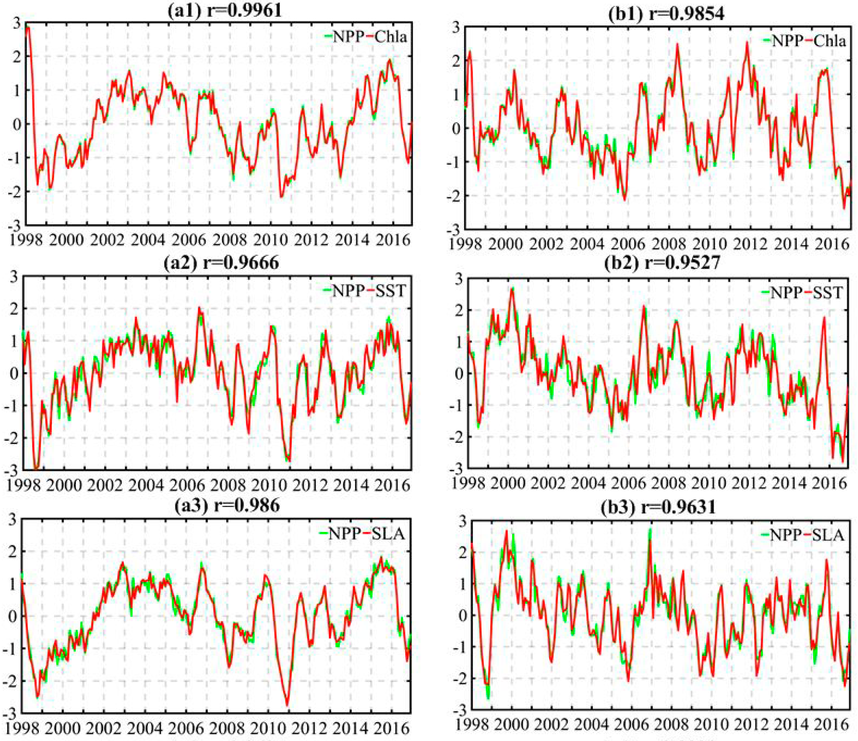
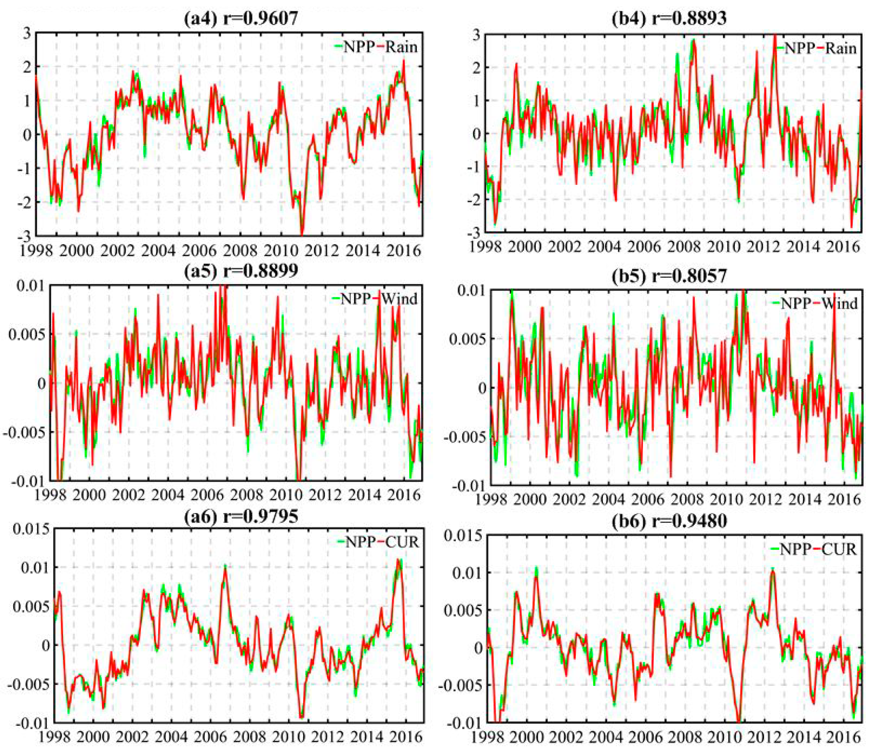
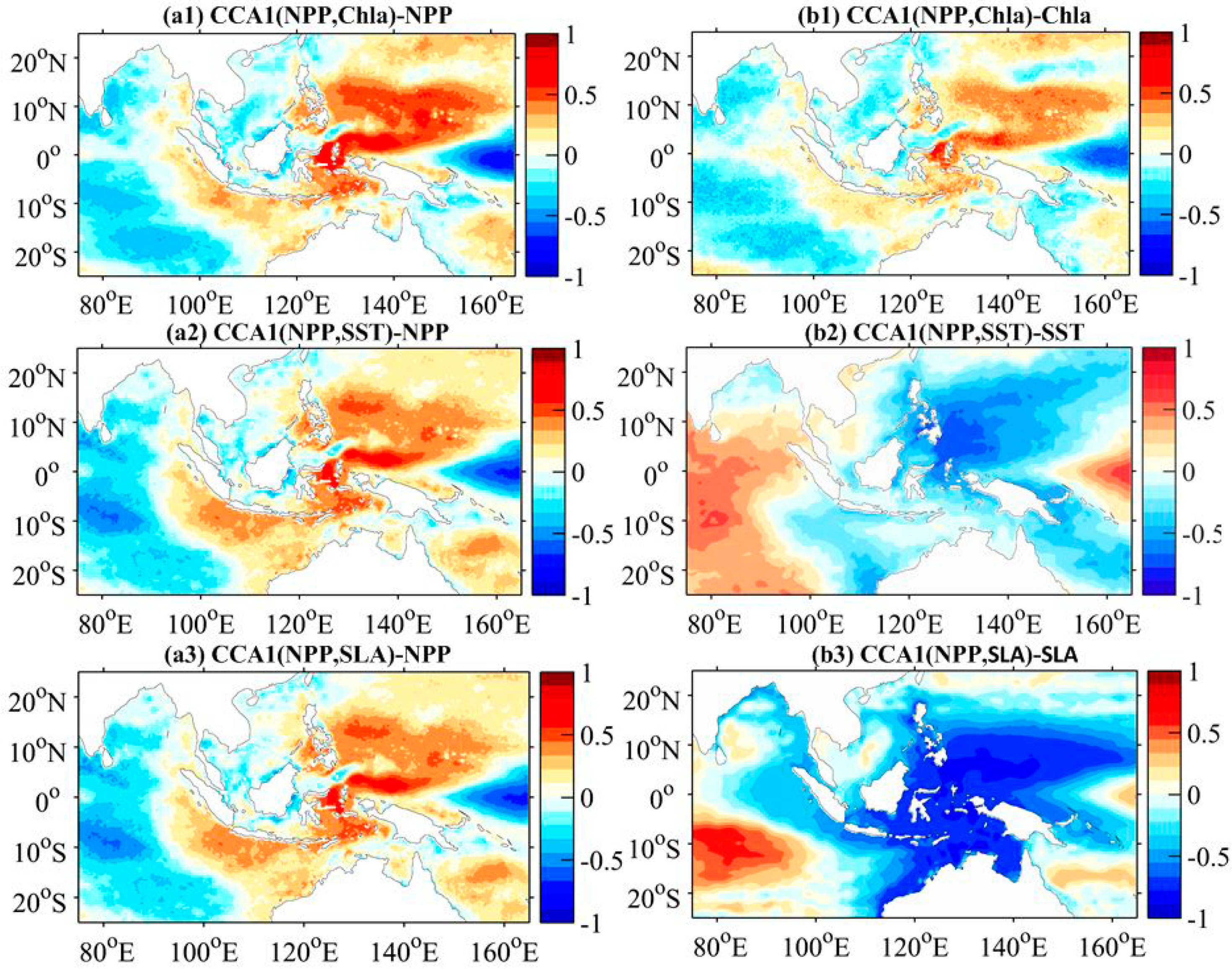
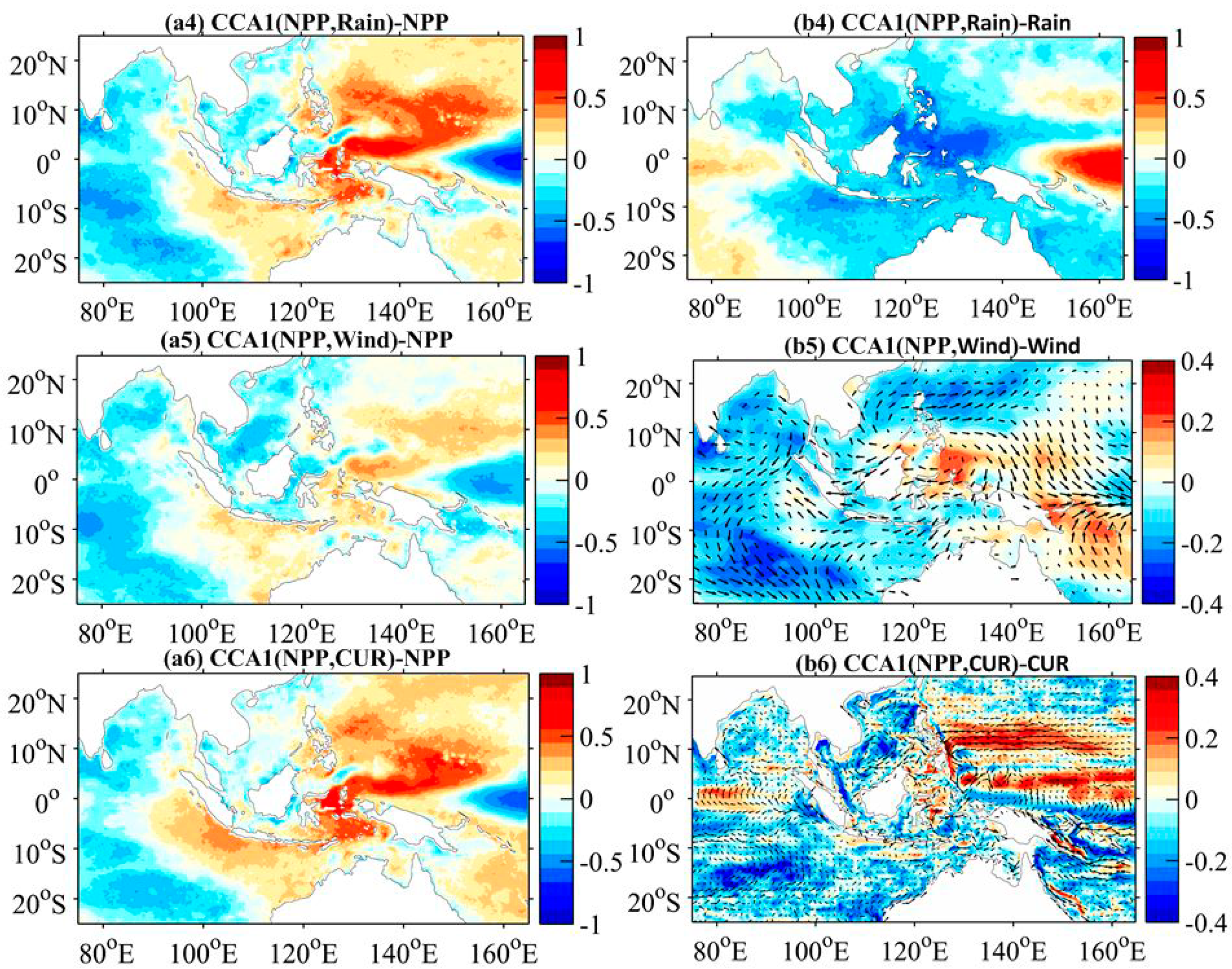
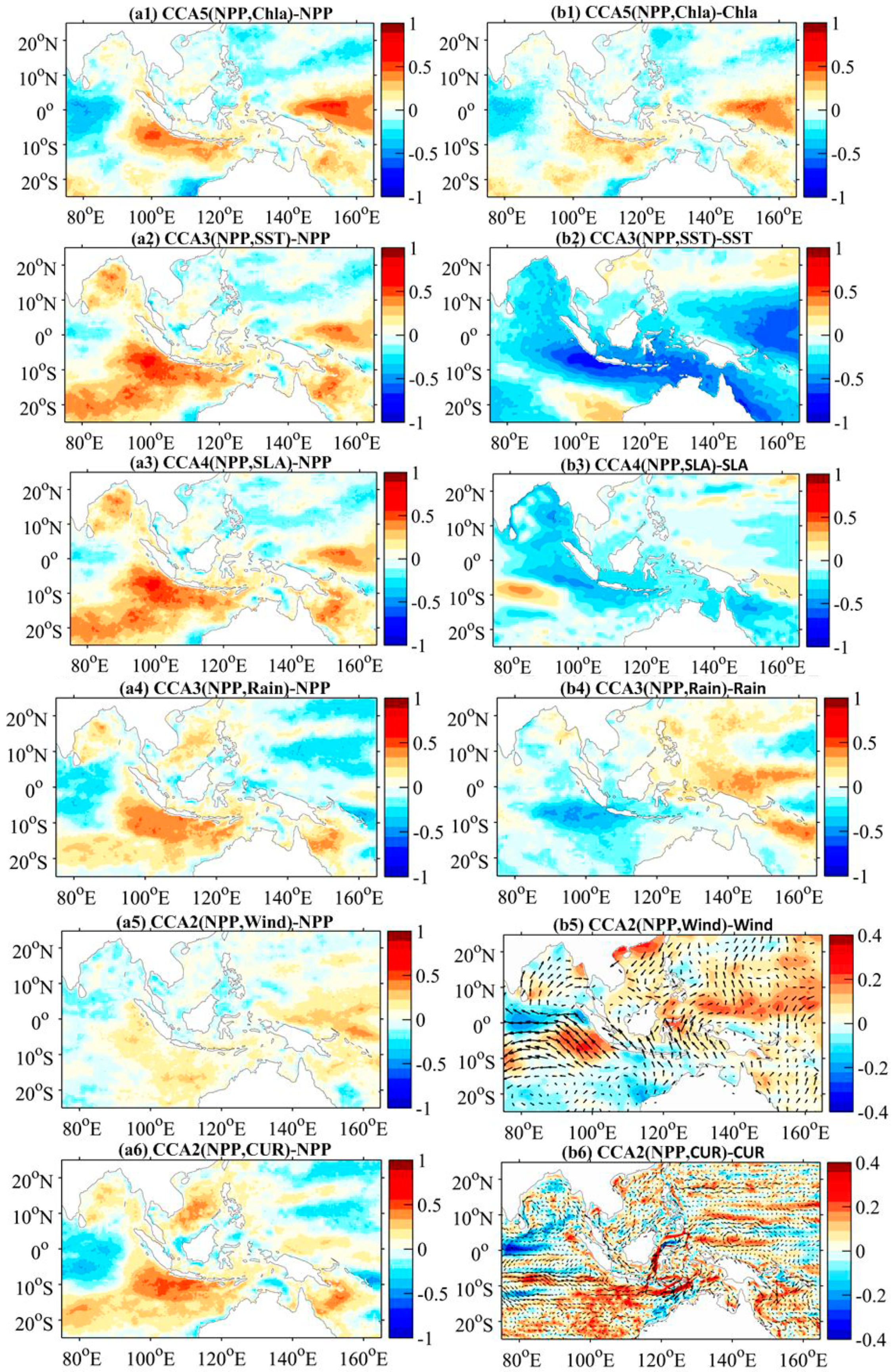
3.4. Covariability Patterns of NPP with Major Forcing Factors on Interannual Timescale

We compiled the coupled patterns of NPP with typical environmental variables (Chla, SST, SLA, Rain, Wind, and CUR) using the BPCCA analysis to understand different covariability patterns under the influence of ENSO and IOD. The correlation coefficient maps of canonical coupled patterns labeled as CCA (NPP, Chla), CCA (NPP, SST), CCA (NPP, SLA), CCA (NPP, Rain), CCA (NPP, Wind), and CCA (NPP, CUR) associated with ENSO and IOD separately are displayed in Figure 9 and Figure 10, respectively. Their corresponding temporal variations are shown in Figure 8. The correlation coefficients of the canonical time series with MEI and DMI are shown in Table 4.
For the first coupled modes of NPP with all environmental variables, the canonical time series closely correlated with MEI indicates that these dominant covariability modes are associated with ENSO (Table 4). In addition, the canonical time series value differences also deliver the intensity of El Niño and La Niña events (Figure 8a1–a6). With respect to the spatial patterns, NPP strongly coupled with Chla, SST, SLA, Rain, Wind, and CUR on interannual timescales is discovered (Figure 9a1–a6,b1–b6). These NPP spatial patterns are similar to the second EOF spatial pattern presented in Figure 4a, meaning that the BPCCA results are credible.
The highly correlated feature in Figure 9 reveals a basin-scale decrease in NPP in the southern SCS and western BoB as well as the equatorial Pacific east of 155°E and the central southern Indian Ocean during El Niño years (2002–2003, 2004–2005, 2006–2007, 2009–2010, and 2014–2016), where NPP and Chla are anomalously negative in concert with sensitive responses to ENSO (Figure 9a1,b1). Meanwhile, El Niño induces the elevated SST and SLA and increased rainfall in the open seas of the equatorial Pacific east of 155°E and the central southern Indian Ocean (Figure 9a2–a4,b2–b4), which strengthens the ocean stratification and deepens the thermocline leading to reduced mixing efficiency and inhibited vertical nutrient inputs into the euphotic layer, as well as reduces the solar radiation resulted in the decreased phytoplankton production. However, in coastal regions of the southern SCS and western BoB, negative NPP is closely correlated with negative rain anomalies, which reveals that the decreased rainfall leading to the reduction in nutrients from the river discharge directly is greater than that of the impact of the solar radiation in these areas [38,39]. The formation and intensification of the Ekman convergence indicated by anticyclonic wind and current is clearly observed in the southern SCS, the western BoB and the central southern Indian Ocean (Figure 9a5–a6,b5–b6), which is known to result in a reduced NPP as a consequence of downwelling. Whereas in the equatorial Pacific east of 155°E, despite the westerly wind blast near the New Guinea during El Niño, the zonal advection of nutrient-rich waters originating from the Indonesian coast could not reach the zone in the east of 155°E along the equator [38]. These combined effects of the deepening thermocline, weak vertical mixing, formative downwelling, reduced river discharge, and solar radiation can explain why NPP decreased in the southern SCS and western BoB as well as the equatorial Pacific east of 155°E and the central southern Indian Ocean during El Niño years.
Increased NPP is also observed in the seas of eastern Philippines and northern New Guinea, the Banda-Arafura Sea and the northeastern coasts of Australia, as well as coasts off Sumatra and Java during El Niño years, cooccurring with positive Chla, wind and current speed as well as negative rainfall, SST and SLA. The cold SST and low SLA are generally associated with the weak ocean stratification and shoaling thermocline layer favoring entrainment nutrients to the upper ocean, which leads to substantially NPP increase in these areas during El Niño years. Meanwhile, the reduced rainfall diminishing the effect on the surface solar radiation and photosynthesis enhances the higher NPP [40]. In addition, we can observe the prominent northwesterly wind burst near the New Guinea and the intensified North Equatorial Current and Countercurrent in the eastern Philippines which induces considerable upwelling and offshore advection favoring nutrient-rich deep water to the surface and nutritional water from the western coasts, triggering the phytoplankton bloom [17,28]. Therefore, the increased NPP in the eastern Philippines and northern New Guinea seas during El Niño years could be attributed to the shoaling of the thermocline depth, the reduced rainfall, the prominent northwesterly wind burst and the enhanced North Equatorial Current and Countercurrent favoring for upwelling and offshore advection. Nevertheless, El Niño-induced easterly winds and coastal currents off the coasts of Sumatra and Java are weaker, which shoals the thermocline depth, brings cold water to the surface, and causes relatively weaker NPP augmentation. Moreover, during La Niña years (1998–2000, 2000–2001, 2007–2008, 2010–2011, and 2011–2012), the situation is opposite to that observed during El Niño years.
For the fifth mode of CCA (NPP, Chla), the third mode of CCA (NPP, SST) and CCA (NPP, Rain), the fourth mode of CCA (NPP, SLA), the second mode of CCA (NPP, Wind) and CCA (NPP, CUR) shown in Figure 10, the canonical time series are closely correlated with DMI (Table 4). Therefore, these coupled modes can be regarded as the dominant interannual covariability associated with IOD. This is credible with the similar spatial patterns of NPP presented in Figure 10a1–a6 and Figure 4b.
As is shown in Figure 10, a close correspondence of positive NPP and Chla anomalies is observed off the coasts of Sumatra and Java, the central southern Indian Ocean, and the BoB as well as the southern SCS and coasts off New Guinea and the Solomon Islands during positive IODs (2006, 2007, 2008, 2011, 2012, and 2015). Off the coasts of Sumatra and Java, the cold SST and low SLA cause a shallower thermocline and variations in mixed layer depth triggering strong vertical mixing and bringing highly nutritional water to the surface (Figure 10b2,b3). The reduced rainfall also contributes a lot to the increased NPP through promoting the solar radiation and photosynthesis (Figure 10b4). The stronger southeast winds along Sumatra and Java coasts strengthen the offshore currents and provide favorable conditions for the formation of coastal upwelling leading to enhanced biological productivity during positive IODs (Figure 10b5,b6) [41]. Moreover, we can find that the upwelling regions are also influenced by nutrient inputs associated with the stronger Indonesian Throughflow (ITF) through the Lombok and Ombai Straits. Briefly, the shallower thermocline, stronger vertical mixing, the less rainfall and the upwelling caused by the strong southeast winds and offshore currents, as well as the stronger ITF are responsible for the increased NPP off the coasts of Sumatra and Java during positive IODs.
In the BoB, coastal trapped Kelvin waves during positive IODs results in lower SST and SLA anomalies, which leads to the shallower thermocline and weaker barrier layer favoring for the transport of subsurface high-nutrient water to the surface and causing the increased NPP [42]. Meanwhile, we can observe the increased NPP in the southern SCS and coasts off New Guinea and the Solomon Islands association with the positive IODs, with contributions of the cold SST, low SLA, increased rainfall and the cyclone circulation anomalies, producing increased nutrient availability for phytoplankton growth. However, along the equator in the Indian Ocean, the strong easterly wind and current anomalies induces equatorial convergence zone and forces anomalous downwelling Rossby, which deepens the thermocline and leads to the decreased NPP during positive IODs. The reverse covariability patterns occur over similar regions during negative IODs (1998, 2005, 2010, 2013, and 2016).

4. Discussion

In the study, we have analyzed the seasonal, interannual, long-term, and multiscale variability oscillation patterns of NPP over the tropical eastern Indian and western Pacific Ocean. Spatiotemporal changes of NPP are generally caused by variations of phytoplankton biomass and environmental factors including light, nutrient salt, water temperature, and disturbance, which can be indicated by variables of Chla, SST, SLA, Rain, Wind, and CUR [12,28]. To investigate the dominant mechanisms driving the diverse biophysical interactions associated with ENSO and IOD, we find that the combined effects of the deepening thermocline, weak vertical mixing, formative downwelling, reduced river discharge and solar radiation process could explain why NPP decreases in the southern SCS and western BoB as well as the equatorial Pacific east of 155°E and the central southern Indian Ocean during El Niño years. However, the increased NPP in the eastern Philippines and northern New Guinea seas during El Niño years could be attributed to the shoaling of the thermocline depth, the reduced rainfall, the prominent northwesterly wind burst and the enhanced North Equatorial Current and Countercurrent favoring for upwelling and offshore advection, which is in good accord with the ones published by Hou et al. [17]. Nevertheless, El Niño-induced relatively weaker easterly winds and coastal currents off the coasts of Sumatra and Java cause weaker NPP augmentation.
The shallower thermocline, stronger vertical mixing, less rainfall, and the upwelling caused by the stronger southeast winds and offshore currents, as well as the stronger ITF are responsible for the increased NPP off the coasts of Sumatra and Java during positive IODs, consistent with results of previous studies [6,7,10]. Meanwhile, the increased NPPs in the southern SCS and coasts off New Guinea and the Solomon Islands during positive IODs are contributions of the cold SST, low SLA, increased rainfall and the cyclone circulation anomalies producing increased nutrient availability for phytoplankton growth. The increased NPP in the BoB and the decreased NPP along the equator in the Indian Ocean during positive IODs are due to the coastal trapped Kelvin waves and anomalous downwelling Rossby, respectively.
In addition, studies have suggested that VGPM predicts larger NPP in temperate and subpolar regions and lower values in equatorial regions compare to Eppley-VGPM [24,25,26,27], which may lead to deviation of the NPP variability in the tropical eastern Indian and western Pacific Ocean. Therefore, we will concentrate on studying the NPP estimates model to get more precise NPP products for the study area in the future work.

5. Conclusions

The key Indo-Pacific Warm Pool region has the diversity and complexity of large-scale biophysical interactions. In the study, the seasonal to interannual and long-term NPP variability over the tropical eastern Indian and western Pacific Ocean are analyzed through the EOF, the lead–lag correlation and the EEMD analyses, based on continuous satellite observation and reanalysis datasets for 1998–2016. We find that NPP variations present obviously temporal and meridional differences on seasonal timescales, as NPP reaches peaks approximately three months later in the western Pacific than that of in the eastern Indian Ocean. On interannual timescales, the NPP variability are closely correlated with ENSO (two-month lag) and IOD (synchronization). Furthermore, the long-term trend of NPP on a point-by-point basis using the linear regression reveals an apparent negative trend in the study area. Using EEMD analysis, we find different varying tendencies and similar multiscale oscillation patterns in subregions of the Bay of Bengal (BoB), the South China Sea (SCS), the southeastern Indian Ocean, and the northwestern Pacific Ocean. The spatiotemporal NPP covariability patterns with variables of the Chla, SST, SLA, Rain, Wind, and CUR are assessed in detail using the BPCCA analysis to explain the dominant mechanisms driving the diverse biophysical interactions associated with ENSO and IOD. NPP variability exhibits strong negative correlations with SST, SLA, and Rain anomalies, as well as positive correlations with Chla, Wind, and CUR in general, though the coupling relationship and intensity largely varied on a regional basis. The observed modifications of NPP with major forcing factors under the effects of ENSO and IOD events in the Indo-Pacific Warm Pool region could help improve our understanding of the projected impacts of long-term climate changes on the marine ecosystem and physical dynamics.

Author Contributions

F.K. carried out the research and prepared the manuscript under the guidance of Q.D., K.X. and Z.Y. contributed to the preparation of the paper through review, editing, and comments. Y.L. and J.L. completed data downloading and image plotting. All authors made substantial intellectual contributions to the paper and the findings reported herein.

Funding

This research was supported by the National Key Research and Development Program of China (2017YFA0603003), the strategic pilot technology project (class A) of the Chinese Academy of Sciences (XDA19060504), and the National Natural Science Foundation of China (NO. 41876210).

Acknowledgments

The Standard VGPM NPP datasets is provided by the Ocean Productivity site (www.science.oregonstate.edu/ocean.productivity). The Chla data is provided by the Ocean Colour Climate Change Initiative (www.esa-oceancolour-cci.org). The SST data is from the NOAA/OAR/ESRL PSD (www.esrl.noaa.gov/psd). The SLA data is from the Archiving, Validation and Interpretation of Satellite Oceanographic data (www.aviso.altimetry.fr/en/data/products/sea-surface-height-products.html). The rainfall data is provided by the NASA Goddard Earth Sciences Data and Information Services Center (https://mirador.gsfc.nasa.gov/). The wind product is from the Remote Sensing Systems (www.remss.com). The current data is provided by the Copernicus Marine Environment Monitoring Service (http://marine.copernicus.eu/). The MEI and DMI are from NOAA (www.esrl.noaa.gov/psd/enso/mei/) and (www.esrl.noaa.gov/psd/gcos_wgsp/Timeseries/DMI/). We are grateful to the Ocean Productivity, ESA, NOAA, AVISO, NASA, RSS, and CMEMS for access to these data.

Conflicts of Interest

The authors declare no conflict of interest.

References

  1. Behrenfeld, M.J.; O’Malley, R.T.; Siegel, D.A.; McClain, C.R.; Sarmiento, J.L.; Feldman, G.C.; Milligan, A.J.; Falkowski, P.G.; Letelier, R.M.; Boss, E.S. Climate-driven trends in contemporary ocean productivity. Nature 2006, 444, 752–755. [Google Scholar] [CrossRef]
  2. Chavez, F.P.; Messié, M.; Pennington, J.T. Marine primary production in relation to climate variability and change. Ann. Rev. Mar. Sci. 2010, 3, 227–260. [Google Scholar] [CrossRef]
  3. Joo, H.T.; Son, S.H.; Park, J.W.; Kang, J.J.; Jeong, J.Y.; Lee, C.I.; Kang, C.K.; Sang, H.L. Long-Term Pattern of Primary Productivity in the East/Japan Sea Based on Ocean Color Data Derived from MODIS-Aqua. Remote Sens. 2016, 8, 25. [Google Scholar] [CrossRef]
  4. Rousseaux, C.S.; Gregg, W.W. Interannual variation in phytoplankton primary production at a global scale. Remote Sens. 2013, 6, 1–19. [Google Scholar] [CrossRef]
  5. Roxy, M.K.; Modi, A.; Murtugudde, R.; Valsala, V.; Panickal, S.; Kumar, S.P.; Ravichandran, M.; Vichi, M.; Lévy, M. A reduction in marine primary productivity driven by rapid warming over the tropical Indian Ocean. Geophys. Res. Lett. 2016, 43, 826–833. [Google Scholar] [CrossRef] [Green Version]
  6. Wiggert, J.D.; Vialard, J.; Behrenfeld, M.J. Basinwide modification of dynamical and biogeochemical processes by the positive phase of the Indian Ocean Dipole during the SeaWiFS era. Indian Ocean Biogeochem. Process. Ecolog. Variab. 2009, 185, 385–407. [Google Scholar] [CrossRef]
  7. Currie, J.; Lengaigne, M.; Vialard, J.; Kaplan, D.; Aumont, O.; Naqvi, S.; Maury, O. Indian Ocean dipole and El Nino/southern oscillation impacts on regional chlorophyll anomalies in the Indian Ocean. Biogeosciences 2013, 10, 6677–6698. [Google Scholar] [CrossRef]
  8. Susanto, R.D.; Moore, T.S.; Marra, J. Ocean color variability in the Indonesian Seas during the SeaWiFS era. Geochem. Geophys. Geosys. 2006, 7. [Google Scholar] [CrossRef] [Green Version]
  9. McCreary, J.; Murtugudde, R.; Vialard, J.; Vinayachandran, P.; Wiggert, J.D.; Hood, R.R.; Shankar, D.; Shetye, S. Biophysical processes in the Indian Ocean. Indian Ocean Biogeochem. Process. Ecolog. Variab. 2009, 185, 9–32. [Google Scholar]
  10. Iskandar, I.; Rao, S.; Tozuka, T. Chlorophyll-a bloom along the southern coasts of Java and Sumatra during 2006. Int. J. Remote Sens. 2009, 30, 663–671. [Google Scholar] [CrossRef]
  11. Hood, R.R.; Beckley, L.E.; Wiggert, J.D. Biogeochemical and ecological impacts of boundary currents in the Indian Ocean. Prog. Oceanogr. 2017, 156, 290–325. [Google Scholar] [CrossRef]
  12. George, J.V.; Nuncio, M.; Chacko, R.; Anilkumar, N.; Noronha, S.B.; Patil, S.M.; Pavithran, S.; Alappattu, D.P.; Krishnan, K.; Achuthankutty, C. Role of physical processes in chlorophyll distribution in the western tropical Indian Ocean. J. Mar. Syst. 2013, 113, 1–12. [Google Scholar] [CrossRef]
  13. Strutton, P.G.; Coles, V.J.; Hood, R.R.; Matear, R.J.; McPhaden, M.J.; Phillips, H.E. Biogeochemical variability in the central equatorial Indian Ocean during the monsoon transition. Biogeosciences 2015, 12, 2367–2382. [Google Scholar] [CrossRef]
  14. Siswanto, E.; Tanaka, K. Phytoplankton Biomass Dynamics in the Strait of Malacca within the Period of the SeaWiFS Full Mission: Seasonal Cycles, Interannual Variations and Decadal-Scale Trends. Remote Sens. 2014, 6, 2718–2742. [Google Scholar] [CrossRef] [Green Version]
  15. Gierach, M.M.; Messié, M.; Lee, T.; Karnauskas, K.B.; Radenac, M.H. Biophysical responses near equatorial islands in the Western Pacific Ocean during El Nino/La Nina transitions. Geophys. Res. Lett. 2013, 40, 5473–5479. [Google Scholar] [CrossRef]
  16. Ryan, J.P.; Ueki, I.; Chao, Y.; Zhang, H.; Polito, P.S.; Chavez, F.P. Western Pacific modulation of large phytoplankton blooms in the central and eastern equatorial Pacific. J. Geophys. Res. Biogeosci. 2006, 111. [Google Scholar] [CrossRef] [Green Version]
  17. Hou, X.; Dong, Q.; Xue, C.; Wu, S. Seasonal and interannual variability of chlorophyll-a and associated physical synchronous variability in the western tropical Pacific. J. Mar. Syst. 2016, 158, 59–71. [Google Scholar] [CrossRef]
  18. Radenac, M.-H.; Messié, M.; Léger, F.; Bosc, C. A very oligotrophic zone observed from space in the equatorial Pacific warm pool. Remote Sens. Environ. 2013, 134, 224–233. [Google Scholar] [CrossRef] [Green Version]
  19. Turk, D.; Meinen, C.; Antoine, D.; McPhaden, M.; Lewis, M. Implications of changing El Niño patterns for biological dynamics in the equatorial Pacific Ocean. Geophys. Res. Lett. 2011, 38. [Google Scholar] [CrossRef] [Green Version]
  20. Ayers, J.M.; Strutton, P.G.; Coles, V.J.; Hood, R.R.; Matear, R.J. Indonesian throughflow nutrient fluxes and their potential impact on Indian Ocean productivity. Geophys. Res. Lett. 2014, 41, 5060–5067. [Google Scholar] [CrossRef] [Green Version]
  21. Behrenfeld, M.J.; Falkowski, P.G. Photosynthetic Rates Derived from Satellite-Based Chlorophyll Concentration. Limnol. Oceanogr. 1997, 42, 1–20. [Google Scholar] [CrossRef]
  22. Campbell, J.; Antoine, D.; Armstrong, R.; Arrigo, K.; Balch, W.; Barber, R.; Behrenfeld, M.; Bidigare, R.; Bishop, J.; Carr, M.E. Comparison of algorithms for estimating ocean primary production from surface chlorophyll, temperature, and irradiance. Global Biogeochem. Cycl. 2002, 16, 1–15. [Google Scholar] [CrossRef]
  23. Carr, M.; Friedrichs, M.; Schmeltz, M.; Noguchi, A.; Antoine, D.; Arrigo, K.; Asanuma, I.; Aumont, O.; Barber, R.; Behrenfeld, M. A comparison of global estimates of marine primary production from ocean color. Deep-Sea Res. Part II 2006, 53, 741–770. [Google Scholar] [CrossRef] [Green Version]
  24. Taboada, F.G.; Barton, A.D.; Stock, C.A.; Dunne, J.; John, J.G. Seasonal to interannual predictability of oceanic net primary production inferred from satellite observations. Prog. Oceanogr. 2019, 170, 28–39. [Google Scholar] [CrossRef]
  25. Liao, X.; Ma, J.; Zhan, H. Effect of different types of El Niño on primary productivity in the South China Sea. Aquat. Ecosyst. Health Manag. 2012, 15, 135–143. [Google Scholar] [CrossRef] [Green Version]
  26. Xue, C.; Song, W.; Qin, L.; Dong, Q.; Wen, X. A spatiotemporal mining framework for abnormal association patterns in marine environments with a time series of remote sensing images. Int. J. Appl. Earth Obs. Geoinf. 2015, 38, 105–114. [Google Scholar] [CrossRef]
  27. Venegas, S.; Mysak, L.; Straub, D. Atmosphere–ocean coupled variability in the South Atlantic. J. Clim. 1997, 10, 2904–2920. [Google Scholar] [CrossRef]
  28. Messié, M.; Chavez, F.P. A global analysis of ENSO synchrony: The oceans’ biological response to physical forcing. J. Geophys. Res. Oceans 2012, 117. [Google Scholar] [CrossRef]
  29. North, G.R.; Bell, T.L.; Cahalan, R.F.; Moeng, F.J. Sampling errors in the estimation of empirical orthogonal functions. Month. Weath. Rev. 1982, 110, 699–706. [Google Scholar] [CrossRef]
  30. Henson, S.A.; Sarmiento, J.L.; Dunne, J.P.; Bopp, L.; Lima, I.D.; Doney, S.C.; John, J.G.; Beaulieu, C. Detection of anthropogenic climate change in satellite records of ocean chlorophyll and productivity. Biogeosciences 2010, 7, 621–640. [Google Scholar] [CrossRef] [Green Version]
  31. Huang, N.E.; Wu, Z. A review on Hilbert-Huang transform: Method and its applications to geophysical studies. Rev. Geophys. 2008, 46. [Google Scholar] [CrossRef] [Green Version]
  32. Palacz, A.P.; Xue, H.; Armbrecht, C.; Zhang, C.; Chai, F. Seasonal and inter-annual changes in the surface chlorophyll of the South China Sea. J. Geophys. Res. Oceans 2011, 116. [Google Scholar] [CrossRef] [Green Version]
  33. Zhang, M.; Zhang, Y.; Shu, Q.; Zhao, C.; Wang, G.; Wu, Z.; Qiao, F. Spatiotemporal evolution of the chlorophyll a trend in the North Atlantic Ocean. Sci. Total Environ. 2018, 612, 1141–1148. [Google Scholar] [CrossRef]
  34. Barnett, T.; Preisendorfer, R. Origins and levels of monthly and seasonal forecast skill for United States surface air temperatures determined by canonical correlation analysis. Month. Weath. Rev. 1987, 115, 1825–1850. [Google Scholar] [CrossRef]
  35. Li, Q.; Wei, F.; Li, D. Interdecadal variation of East Asian summer monsoon and drought/flood distribution over eastern China in the last 159 years. Acta Geograp. Sin. 2011, 21, 579–593. [Google Scholar] [CrossRef]
  36. Bretherton, C.S.; Smith, C.; Wallace, J.M. An intercomparison of methods for finding coupled patterns in climate data. J. Clim. 1992, 5, 541–560. [Google Scholar] [CrossRef]
  37. Storch, H.V.; Zwiers, F.; Livezey, R. Statistical analysis in climate research. Nature 2000, 404, 544. [Google Scholar]
  38. Krüger, O.; Graßl, H. Southern Ocean phytoplankton increases cloud albedo and reduces precipitation. Geophys. Res. Lett. 2011, 38. [Google Scholar] [CrossRef] [Green Version]
  39. Tang, D.; Kawamura, H.; Van Dien, T.; Lee, M. Offshore phytoplankton biomass increase and its oceanographic causes in the South China Sea. Mar. Ecol. Prog. Ser. 2004, 268, 31–41. [Google Scholar] [CrossRef] [Green Version]
  40. Park, J.Y.; Kug, J.S.; Park, J.; Yeh, S.W.; Chan, J.J. Variability of chlorophyll associated with El Niño–Southern Oscillation and its possible biological feedback in the equatorial Pacific. J. Geophys. Res. Oceans 2011, 116. [Google Scholar] [CrossRef] [Green Version]
  41. Vinayachandran, P.N.; Francis, P.A.; Rao, S.A. INDIAN OCEAN DIPOLE: PROCESSES AND IMPACTS. Curr. Trend. Sci. 2009, 569–589. [Google Scholar]
  42. Girishkumar, M.S.; Ravichandran, M.; Pant, V. Observed chlorophyll-a bloom in the southern Bay of Bengal during winter 2006–2007. Int. J. Remote Sens. 2012, 33, 1264–1275. [Google Scholar] [CrossRef]
Figure 1. Climatological ocean net primary production (NPP) during 1998–2016 in the study area, derived based on SeaWiFS and MODIS Chla using the VGPM algorithm.
Remotesensing 11 00391 g001
Figure 2. Seasonal NPP variability characterized by the first two EOF modes: (a,b) are the EOF spatial patterns (Unit: log10, mg C/m2/month); (c,d) are the time series of normalized principal components (PC).
Remotesensing 11 00391 g002
Figure 3. Interannual NPP variability characterized by the first EOF mode: (a) the EOF spatial pattern; (b) the normalized PC (red) along with MEI (blue) and DMI (green).
Remotesensing 11 00391 g003
Figure 4. Interannual NPP variability characterized by the second and third EOF modes: (a,b) the EOF spatial patterns; (c,d) the normalized PC (red) along with MEI (blue) and DMI (green); (e,f) the lagged correlations of PC with MEI and DMI, respectively.
Remotesensing 11 00391 g004
Figure 5. Long-term NPP trend during the period of 1998–2016. Points plotted are the statistically significant values (p < 0.1).
Remotesensing 11 00391 g005
Figure 6. Significance tests of IMFs in the (a) Bay of Bengal (BoB), (b) South China Sea (SCS), (c) southeastern Indian Ocean, (d) northwestern Pacific Ocean. Statistically significant IMFs were placed above the diagonal lines for the 95% (blue line) and 90% significance levels (magenta line).
Remotesensing 11 00391 g006
Figure 7. Raw time series (solid line in the top panel), trend (dashed red line in the top panel), and the significant IMFs for domain-averaged NPP (mg C/m2/month) in the (a) BoB, (b) SCS, (c) southeastern Indian Ocean, (d) northwestern Pacific Ocean.
Remotesensing 11 00391 g007
Figure 8. The time series and correlation coefficient of canonical coupled BPCCA modes associated with ENSO (left panel) and IOD (right panel), respectively. (a1) the canonical time series of NPP (green line) and Chla (red line) associated with ENSO, (b1) the canonical time series of NPP (green line) and Chla (red line) associated with IOD. (a2a6,b2b6) are the same as (a1,b1) but for the modes of NPP with SST, SLA, Rain, Wind, and CUR.
Remotesensing 11 00391 g008aRemotesensing 11 00391 g008b
Figure 9. The canonical coupled BPCCA modes associated with ENSO. (a1,b1) spatial correlation patterns of NPP and Chla for the first canonical pair labeled as CCA1 (NPP, Chla)-NPP and CCA1 (NPP, Chla)-Chla, respectively. (a2a6,b2b6) are the same as (a1,b1) but for the modes of NPP with SST, SLA, Rain, Wind, and CUR, respectively.
Remotesensing 11 00391 g009aRemotesensing 11 00391 g009b
Figure 10. Same as Figure 9, but for the canonical coupled CCA modes associated with IOD. (a1,b1) spatial correlation patterns of NPP and Chla for the fifth canonical pair labeled as CCA5 (NPP, Chla)-NPP and CCA5 (NPP, Chla)-Chla, respectively. (a2a6,b2b6) are similar as (a1,b1) but for the modes of NPP with SST, SLA, Rain, Wind, and CUR, respectively.
Remotesensing 11 00391 g010
Table 1. Sources, timespans, and temporal–spatial resolutions of the datasets.
VariableData SourceTimespanResolution
NPPSeaWiFS/MODIS Standard VGPMOct 1997–present9 km, monthly
ChlaOC-CCI V3.1Sep 1997–present4 km, monthly
SSTOI SST V2Dec 1981–present0.25°, daily
SLAAVISODec 1992–present0.25°, monthly
RainTRMM_3B43 V7Jan 1998–present0.25°, monthly
WindCCMP V2.0Jan 1987–present0.25°, monthly
CURCMEMSJan 1993–Dec 20160.083°, monthly
Table 2. Correlations of the first three principal components (PC1, PC2 and PC3) with MEI and DMI.
IndicesPC1PC2PC3
MEI0.460.650.05
DMI0.230.100.48
Table 3. The mean periods and variance contribution rates of the significant IMFs for domain-averaged NPP in the BoB, SCS, southeastern Indian Ocean, and northwestern Pacific Ocean.
RegionsIMFMean Period/Month (Year)Variance Contribution Rate/%
BoBC210.43 29.16
C431.76 (2.6a) 8.04
C6233.22 (19.4a) 1.56
SCSC213.57 56.70
C319.62 (1.6a) 14.98
C473.41 (6.1a) 4.12
southeastern Indian OceanC213.28 82.44
C333.45 (2.8a) 5.90
C494.80 (7.9a) 3.93
C5119.43 (9.9a) 0.56
northwestern Pacific OceanC214.38 78.91
C331.00 (2.6a) 2.68
C461.46 (5.1a) 4.88
C5114.00 (9.5a) 3.67
Table 4. Canonical time series correlation coefficients of biophysical variables with climate-related indices of MEI and DMI.
VariableMEIDMIVariableMEIDMI
CCA1 (NPP, Chla)-NPP0.810.01CCA5 (NPP, Chla)-NPP0.200.45
CCA1 (NPP, Chla)-Chla0.810.01CCA5 (NPP, Chla)-Chla0.210.45
CCA1 (NPP, SST)-NPP0.680.39CCA3 (NPP, SST)-NPP0.180.39
CCA1 (NPP, SST)- SST0.650.37CCA3 (NPP, SST)- SST0.180.39
CCA1 (NPP, SLA)-NPP0.750.28CCA4 (NPP, SLA)-NPP0.020.35
CCA1 (NPP, SLA)- SLA0.740.29CCA4 (NPP, SLA)- SLA0.030.36
CCA1 (NPP, Rain)-NPP0.780.27CCA3 (NPP, Rain)-NPP0.240.43
CCA1 (NPP, Rain)- Rain0.760.27CCA3 (NPP, Rain)- Rain0.230.41
CCA1 (NPP, WindUV)-NPP0.350.20CCA2 (NPP, WindUV)-NPP0.180.53
CCA1 (NPP, WindUV)- WindUV0.320.17CCA2 (NPP, WindUV)- WindUV0.190.46
CCA1 (NPP, WindW)-NPP0.360.27CCA3 (NPP, WindW)-NPP0.240.34
CCA1 (NPP, WindW)-WindW0.330.27CCA3 (NPP, WindW)-WindW0.240.26
CCA1 (NPP, CURUV)-NPP0.660.34CCA5 (NPP, CURUV)-NPP0.080.37
CCA1 (NPP, CURUV)-CURUV0.660.35CCA5 (NPP, CURUV)-CURUV0.070.34
CCA1 (NPP, CURW)-NPP0.670.34CCA2 (NPP, CURW)-NPP0.030.45
CCA1 (NPP, CURW)-CURW0.670.33CCA2 (NPP, CURW)-CURW0.030.44

