Local Severe Storm Tracking and Warning in Pre-Convection Stage from the New Generation Geostationary Weather Satellite Measurements

Abstract

Accurate and prior identification of local severe storm systems in pre-convection environments using geostationary satellite imagery measurements is a challenging task. Methodologies for “convective initiation” identification have already been developed and explored for operational nowcasting applications; however, warning of such convective systems using the new generation of geostationary satellite imagery measurements in pre-convection environments is still not well studied. In this investigation, the Random Forest (RF) machine learning algorithm is used to develop a predictive statistical model for tracking and identifying three different types of convective storm systems (weak, medium, and severe) over East Asia by combining spatially-temporally collocated Himawari-8 (H08) measurements and Numerical Weather Prediction (NWP) forecast data. The Global Precipitation Measurement (GPM) gridded product is used as a benchmark to train the predictive models based on a sample-balance technique which can adjust or balance the samples of three different convection types to avoid over-fitting any type of dataset. Variables such as brightness temperatures (BTs) from H08 water vapor absorption bands (6.2 μm, 6.9 μm and 7.3 μm) and Total Precipitable Water (TPW) from NWP show relatively high ranks in the predictive model training. These sensitive variables are closely associated with convectively dominated precipitation areas, indicating the importance of predictors from both H08 and NWP data. The final optimal RF model is achieved with an accuracy of 0.79 for classification of all convective storm systems, while the Probability of Detection (POD) of this model for severe and medium convections can reach 0.66 and 0.70, respectively. Two typical sudden convective storm cases in the warm season of 2018 tracked by this algorithm are described, and results indicate that the H08 and NWP based statistical model using the RF algorithm is capable of capturing local burst convective storm systems about 1–2 h earlier than the outbreak of heavy rainfall.

1. Introduction

Severe convective weather systems are usually accompanied by short-lived heavy rainfall, thunderstorms, strong winds, tornadoes, and/or hailstorms on the order of a dozen to three hundred kilometers horizontally [1]. The emergence or outbreak of convective weather systems often causes significant economic losses. Turbulence and high-altitude ice formation caused by convective weather systems also seriously threaten the aviation safety [2]. Traditionally, operational numerical weather prediction (NWP) model data is used to predict the occurrence of severe convective weather systems [3]. However, for some isolated and sudden local convective storm systems with short lifetimes, it is still hard to accurately predict their occurrence, development, and movement based on the current NWP models [4]. However, severe convective storm systems can be well tracked or observed by geostationary (GEO) weather satellites and/or ground-based weather radars in their initial stages [5], which are always adopted as convective initiation (CI) products in nowcasting applications.

Some previous studies [6,7] have already pointed out that the GEO orbit weather satellites can well capture sudden convective weather systems with a high spatiotemporal resolution. Normally, based on the GEO satellite observations, features and temporal variations at the cloud top from the infrared (IR) brightness temperature (BT or TBB, temperature of black body) observations are used to track and identify developing convective storm systems [6]. Another significant benefit of the IR-based identification method is the ability to perform a unified and continuous recognition of convective storm systems from day to night, without the need to rely on the reflected sunlight [6,8]. However, due to remarkable seasonal, regional, or sensor specification differences, there is no unified IR BT threshold for tracking and identifying potential convective cloud clustering [9]. As early as 1980, Maddox first used 241 K for IR window band as a criterion to identify mesoscale convective cloud systems (MCS) [10]. In the most recent decade, with the rapid improvement of space-based imaging sensors, Laing et al. [11] found that the presence of high altitude cirrus clouds can significantly impact the accuracy of convective storm system identification. Thus they proposed a new marker of 233 K (BT at 10.5–12.5 μm band from the European GEO meteorological Satellite-7, and Meteosat-7) for judging convection. Recently, it was found that MCS lifetimes were impacted by the use of a lower IR threshold identification method. [12]. To further improve the accuracy of the single IR band algorithm for CI detection, the BT gradient of IR window band and tropopause temperature from NWP data were used to further analyze convective storm events [13]. Furthermore, Wang [14] found that the water vapor band plays an important role in cloud classification during nighttime hours. When combining the IR window band and the water vapor absorption band, the accuracy of convection classification is higher than that using only one band [14].

In addition to the temporal variation of BT at the top of cloud deck, some BT differences (BTDs) between different spectral bands were also used for detecting convective storm systems [15]. With the vigorous and rapid development of convective systems, a strong updraft will transport water vapor above convective cloud clusters and break through the top of the troposphere into the lower stratosphere [16]. Ackerman [17] found that when tropospheric water vapor enters the stratosphere, the BTDs at the top of cloud between the water vapor (high BT) and IR window band (low BT) are negative; therefore, he used the BTD between water vaper and IR window band to detect convection systems.

In recent years, China Meteorological Administration (CMA), Japan Meteorological Agency (JMA), and U.S. National Oceanic and Atmospheric Administration (NOAA) have already successfully launched their own new-generation geostationary weather satellites in succession since 2014. The new generation GEO weather satellites, such as Chinese FengYun-4 (FY-4) series [8], Japanese Himawari-8/9 [18], and U.S. Geostationary Operational Environmental Satellites-R (GOES-R) series [19], carrying advanced sensors, provide new opportunities for detecting and tracking severe convective storm systems. New measurements can help to further understand the occurrence and development of convection from a satellite perspective [20]. It is worthy to note that the Himawari-8 was successfully launched on 7 October 2014. It carries a 16-band Visible (VIS) and IR Advanced Himawari Imager (AHI) with spatial resolutions from 0.5 km (VIS) to 2.0 km (IR) and a full-disk observation within a 10-minute time interval (http://www.jma-net.go.jp/msc/en/).

With new measurements from the advanced GEO space-based sensors, some advanced machine learning (ML) techniques, such as random forests (RF), support vector machines (SVM), artificial neural network (ANN), deep learning (DL), etc. that were successfully used to solve non-linear weather-related issues [21,22] and can be used to better understand convective storms. Williams [21] examined the specific problem of combining NWP model, radar, and satellite for forecasting thunderstorm initiation in a one-hour timeframe [21]. These innovative applications are benefited from the rapid development of ML frameworks, such as scikit-learn (http://scikit-learn.org/), Theano (http://deeplearning.net/software/theano/), TensorFlow (http://www.tensorfly.cn/), and PyTorch (https://pytorch.org), which are easy to be implemented for statistical model training and predicting. As one of many accurate and high-efficiency ML algorithms, the Random Forest (RF) has been successfully and extensively utilized in weather and remote sensing applications [23]; it is capable of capturing non-linear relationship between predictors and predictands.

In this study, based on H08/AHI data, the RF learning algorithm is used to develop a near real-time (NRT) tracking and warning predictive model for convective storm systems. The predictive model can capture the sudden local convective systems from a newly-formed cell using high spatiotemporal resolution H08/AHI IR observations, for example, to predict the occurrence and the intensity of convective storm systems using the variables from the spatially-temporally matched H08/AHI observations and GFS (Global Forecast System) NWP data [24]. Unlike the traditional method, some important parameters, such as total precipitable water (TPW), from NWP data are introduced here to provide atmospheric environmental field information for better identifying convective storm systems. By using AHI and the real-time GFS NWP data in the warning algorithm, the convective storm system tracking and identify model called Storm Warning In Pre-convective Environment (SWIPE) has been developed for nowcasting applications [25].

Section 2 introduces the new GEO and GFS NWP data. Section 3 presents the convective-tracking algorithm and collected dataset. Section 4 elaborates the RF classification algorithm, the SWIPE prediction model and its evaluation. Two typical convective storm cases tracked by the SWIPE model are introduced and discussed in Section 5. Finally, Section 6 provides a summary and future work.

2. Data

Seven months of continuous H08 and GFS NWP data (from April to October 2016) are used here to build a robust and efficient convective storm prediction model (SWIPE) with RF algorithm. This period covers the typical summer precipitation season over China. Himawari-8, the next-generation geostationary satellite belonging to the Japan Meteorological Agency (JMA, http://www.jma-net.go.jp/msc/en/), was successfully launched into geosynchronous orbit and centered around 140.7°E on 7 October 2014. The AHI onboard H08 has 16 bands including 4 VIS, 2 near-IR (NIR), and 10 IR bands with central wavelengths ranging from 0.47 to 13.3 µm. It routinely operates a full disk and five sub-region scanning modes within a 10 min (or 2.5 min for a regionally rapid scanning mode) interval with spatial resolutions 0.5 km and 1 km for VIS bands, and 2 km for NIR and IR bands. As a primary H08 data user in China, the China Meteorological Administration (CMA) can obtain the H08/AHI Level-1B data with geolocation and radiometric calibration from JMA in NRT for now-casting applications [25,26,27].

In addition to the radiances at the top of atmosphere observed by H08/AHI, some other important atmospheric environment parameters are also used. The NWP model data, containing global three-dimension (3D) atmospheric environmental parameters such as temperature, humidity, pressure, wind speed, etc., with a horizontal spatial resolution of 0.5° × 0.5° and 26 vertical layers from 1000 hPa to 10 hPa, are routinely generated by the National Centers for Environmental Prediction (NCEP) GFS, a global NWP system containing a global computer model and variational analysis run by NOAA National Weather Service (NWS). A linear interpolation technique is used here to match H08/AHI observations and GFS NWP data, and NWP data are mapped to observations. Based on the NWP data, some environmental parameters (such as TPW, K-Index and Lifted Index) are chosen to train the convective storm prediction model, which are likely to be closely associated with the severe convective weather events [28].

Besides the two datasets mentioned above, we also use the Global Precipitation Measurement (GPM) level three gridded Integrated Multi-satellite Retrievals for GPM (IMERG) V04A version data [29] for reliable training and validation data in this study. The GPM is a joint mission between NASA and JAXA to make frequent observations of global precipitation. It is an important part of NASA’s Precipitation Measurement Missions (PMM) program and works with a satellite constellation to provide full global coverage. As the successor to Tropical Rainfall Measuring Mission (TRMM) mission, the GPM can provide more frequent and accurate observations of global precipitation. As a key sensor, the microwave imager capturs the precipitation intensity and horizontal morphology, while the dual-band precipitation radar provides three-dimensional structure of precipitation aggregates. IMERG is a merged precipitation product based on GPM observations and other satellite microwave precipitation estimates [30], with a half an hour interval and a spatial resolution of 0.1° × 0.1°. It can cover the global area between the latitudes of 60°N and 60°S [31]. This product has been well validated using ground-based gauges or surface based radars [30]. Therefore, the GPM IMERG product is used as the truth for training the SWIPE prediction model based on its high quality.

3. Convective-Tracking Method and Dataset

3.1. Spatial Distributions

In the current study, we focus on the sudden local convective storms observed over China and nearby regions (a domain bracketed from 70°E to 140°E and 15°N to 60°N, see Figure 1), which can be fully covered by H08/AHI data. This region has complex spatial and temporal structures. It covers both subtropical and mid-latitude regions, and its rainfall is often concentrated on long strips stretching for thousands of kilometers, affecting China, Japan, South Korea and the surrounding seas. During the East Asian summer monsoon, the impact of floods on human life and the economy is large, as finer seasonal space-time structures combined with narrow rivers are more sensitive to inter-annual variations [32]. Note that this area of interest includes some typical climate belts, complex atmospheric circulation, and various terrain, such as the tropical monsoon region, the subtropical monsoon climate region, the Qinghai-Tibet plateau climate region, etc. In summertime, the warm and humid air flow from the tropical ocean provides sufficient water and seasonal precipitation to the North of the area, resulting in a large number of strong convective systems, which is conducive to the establishment of a rich data set of strong convection systems [33].

In this study, the rank of convective storm system is divided into three types on the basis of amount of quantitative precipitation, including (1) slight convective storm system with the maximum rain rate less than 2.5 mm/h, (2) medium-strength convection storm system with the maximum rain rate from 2.5 to 16 mm/h, and (3) severe convective storm system with the maximum rain rate exceeding 16 mm/h. The two instantaneous rain rates of 16 and 2.5 mm/h stem from a common classification criterion of heavy rainfall over China by the National Meteorological Center (NMC) of CMA and a standard definition of moderate rain by the American Meteorological Society (AMS) [34].

3.2. Convective-Tracking

Cloud top IR BT variations from two successive images observed by a GEO satellite are used to track convective storm system development, as introduced in Section 1. In this study, in order to better identify developing convective initiation systems, we screen cloud clusters using an IR BT threshold below 273 K at the 10.4 μm band observed by H08/AHI. This IR threshold can help us to further identify potential cloud clusters, which might grow into strong convection systems. After screening warm cloud cluster, a classical area-overlapped method [35] is applied to track the cloud cluster movement based on two consecutive H08/AHI observation data within a 10 min interval. For the tracked cloud system objects, we use the equations (1) and (2) to calculate the two consecutive cloud top cool rates (R) at the 10.4 μm band as follows:

$$R_1=\frac{\min \left(B{T}_{A2,1},B{T}_{A2,2},\dots B{T}_{A2,n}\right)-\min \left(B{T}_{A1,1},B{T}_{A1,2},\dots B{T}_{A1,n}\right)}{t_2-t_1},$$

(1)

$$R_2=\frac{\min \left(B{T}_{A3,1},B{T}_{A3,2},\dots B{T}_{A3,n}\right)-\min \left(B{T}_{A2,1},B{T}_{A2,2},\dots B{T}_{A2,n}\right)}{t_3-t_2},$$

(2)

where the symbol min represents the minimum function. A_{1, 2, 3} and t_{1, 2, 3} mean the tracked and overlapped convective storm cloud cluster area and observation time, respectively. The numbers from one to n denote the pixel number in the cloud cluster area, A₁, A₂, or A₃. If both the cooling rates of R₁ and R₂ reach −16 K/hour or lower [36], the related cloud system will be marked or considered to be a potential or developing convective cloud cluster. To better track sudden convective storm systems and ignore large-scale convective systems (they are always closely associated with frontal cloud systems) [37], the SWIPE model only identifies the convective cloud cluster areas with a total pixel number ranging from 10 to 80,000 (maximum area is about 600 km × 600 km). Thus, three consecutive observation BT images should be used to compute two continuous cloud top cooling rates, which could help the algorithm to better identify the rapidly developing convective cloud clusters.

Figure 2 is an example of this convective-tracking method using three continuous BT images within a 10 min observation interval. It shows a real case of a tracked convective storm system at 19:30 UTC on 05 July 2016 in Guangdong province of China using H08/AHI observations. The small colorful sub-figures in the left panel column represent the 10.4 μm BT images at 19:10, 19:20, and 19:30 UTC, respectively. For this case, it can be seen that the two continuous cloud top cooling rates are less than −16 K/h, and the BT at the coldest part of convective cluster at 19:30 UTC is lower than 200 K. This severe local convective storm system ultimately generated a maximum rain rate of 26.4 mm/h.

3.3. Datasets

As mentioned before, the cooling rate of the IR BTs with spatial resolution of 2 km at the top of cloud cluster observed by H08/AHI, is used to identify the rapidly developing convective storm cluster. After this step, a spatial and temporal matching technique is used to collocate H08/AHI and GPM IMERG data. The GPM IMERG data right after the time when the SWIPE recognizes a convective cloud is used to match the H08/AHI data. For example, if SWIPE recognizes a convective cloud at 07:10 UTC, then the GPM data of 07:30 UTC is used to determine the rain rate of this cloud cluster. A maximum rain rate (from GPM IMERG) from the 10% coldest pixels of potential convective storm cluster is marked as its final rain rate. A temporal linear interpolation technique is also used here to match NWP data (3 h interval) with the collocated H08/AHI and GPM IMERG data. Based on the collocated dataset, all the samples of convective storm systems were tracked and identified from April to October 2016. During this period, a total of 88,351 convective storm events were successfully tracked using the aforementioned method, including 85,102 slight (or none), 2540 medium, and 709 severe convective storm systems.

Table 1. Monthly total numbers of three typical convective storm systems in the area of interest from April to October 2016.

Month	Severe	Medium	Slight (or None)
April	72	82	5426
May	133	266	11,412
June	76	289	10,492
July	78	511	14,019
August	123	497	15,835
September	121	493	16,380
October	106	396	11,538

lists the numbers of three typical convective storm systems tracked from April to October 2016. Similar to Table 1, Figure 1 shows the spatial distributions of three typical convective storm systems during this period. We find significant geographical and seasonal characteristics of convective storm systems over this area. The most frequent occurrences of convective storm systems are presented in July (14,608), August (16,455), and September (16,994). The monthly proportion, reaching 4.17%, of severe and medium storm systems was the highest in October. In this month, 106 severe and 396 medium convective storm systems were found in all of 12,040 potential convective systems. In Figure 1, we also find that the geographic area of strong convection gradually moves North from April to August. Contrarily, it will move toward south at the beginning of September again [38]. It is well known that the seasonal movement pattern of strong convection is closely associated with the Intertropical Convergence Zone (ITCZ) and monsoon [33].

4. Statistical Prediction Model

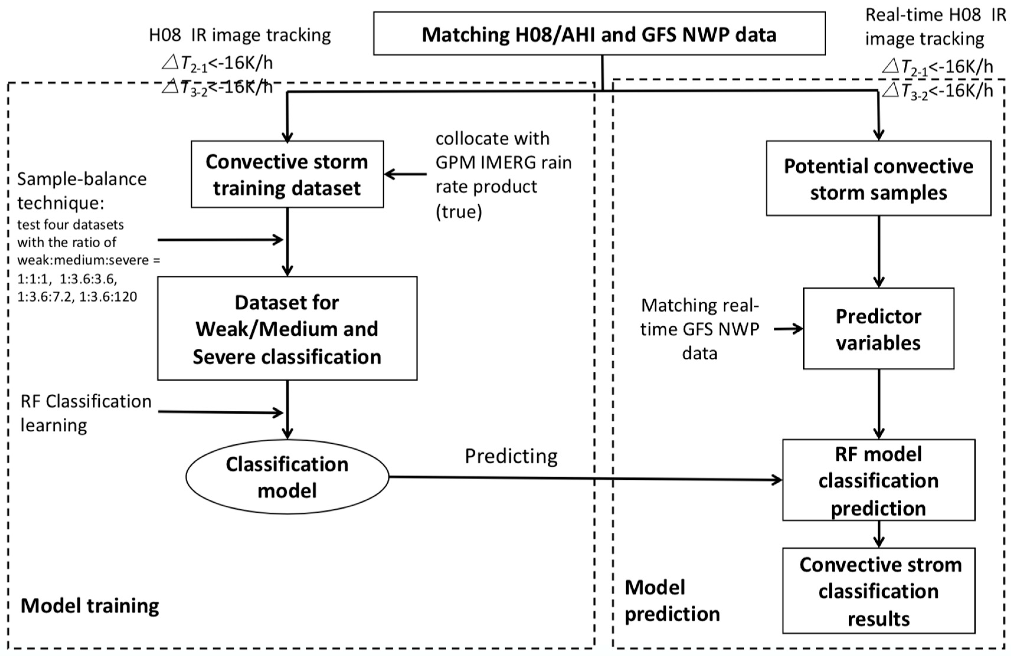
4.1. RF Classification Model Training

Random Forests as an important ensemble and advanced ML algorithm is widely used in data classification and nonparametric regression [39,40]. Here, it is used to build a connection between convective storm system and satellite observations, which can predict the occurrence and intensity of convection. For a detailed introduction to the RF algorithm, please refer to the Appendix A at the end of this paper.

For validating the performance of the RF algorithm based SWIPE model, the data on the 2nd and 15th days of each month are used as independent samples (mentioned in Section 3.3 above) for testing and evaluating the SWIPE model. The test data sets include 47 severe convective systems, 150 medium convective systems and 5498 weak convective systems. These independent data are not included in the training, and the remaining data from April to October of 2016 are used as a training dataset to generating an effective RF classification model — SWIPE. Based on the tracked convective storm system dataset mentioned in Section 3.3, a total of 83 predictive factors (see

Table 2. Predictor variables for the RF classification model training and predicting.

Classification	Variable	Unit
Satellite measurements	T6.2-10.4, T6.9-10.4, T7.3-10.4, T8.6-10.4, T9.6-10.4, T10.4, T11.2-10.4, T12.3-10.4, ∆T13.3-10.4, ∆T8.6-11.2, ∆T11.2-12.3, ∆T3.9-11.2, ∆T3.9-7.3	K
	Area (pixel number of convective storm system)
GFS NWP	K-Index	°C
	CAPE (Convection Available Potential Energy)	J·kg−1
	CIN (Convective Inhibition)	J·kg−1
	LI (Lifted Index)
	EBS (Effective Bulk Shear)	m·s−1
	TPW (Total Precipitable Water)	mm
	${\mathsf{\theta }}_{\mathrm{se}850/925}$ (Pseudo-equivalent potential temperature at 850/925 hPa)	K
	PV (Potential Vorticity)
	Div925/850/10 (Convergence at 925 and 850 hPa/10m)	s−1
	MR850/925 (Mixing Ratio at 850/925 hPa)	g·kg−1

) from H08/AHI observations and spatiotemporally matched NWP data, are used to train the SWIPE model for identifying three different types of convective storm systems, which is one of the key steps for the SWIPE model. According to the previous studies for identifying and tracking convective storm systems [41], the predictors from H08/AHI mainly include the BTs observed by water vapor absorption and IR split window bands. Related studies by Reed et al [42] also indicate that the ECMWF (European Centre for Medium-range Weather Forecasts) analysis data is likely to be able to capture the synoptic-scale and mesoscale features of convective environments. These weather forecast indices can provide a good description of the thermal (K Index), dynamic (CAPE, CIN, Lifted Index, EBS) and moisture (TPW) characteristics of the atmospheric environment. Details of predictors from GFS NWP data used here are listed in Table 2 [43,44].

Note that the total numbers of three different convective systems will affect the final model training and prediction. Previous studies have already pointed out that the sample ratio of different types in the dataset can significantly impact the final accuracy of the prediction model [22,24]. For the original dataset, the natural ratio between severe, medium, and weak convections is about 1:3.6:120, which is also referred to as the original dataset or Scenario-0. When the weak convective systems in the model training are too much, the final prediction will be biased towards this excessive type. In order to further improve the prediction accuracy, the numbers of medium convective systems and weak convective systems are reduced. A variety of scale models were tried to ensure an optimal model. The ratios are adjusted to 1:1:1, 1:3.6:3.6 and 1:3.6:7.2, for three scenarios that are marked as Scenario-1, Scenario-2, and Scenario-3, respectively. This method for adjusting proportions of different types in the dataset is known as the sample-balance technique [45]. By including the original sample scenario,

Table 3. Numbers of weak, medium and severe convections of four typical sample datasets under different scenarios.

	Scenario-1	Scenario-2	Scenario-3	Scenario-0 (Original)
Weak	662	2388	4776	79,549
Medium	662	2388	2388	2388
Severe	662	662	662	662
Proportion	1:1:1	1:3.6:3.6	1:3.6:7.2	1:3.6:120

shows the numbers of weak, medium and severe convections of four typical sample datasets under three different scenarios as described above. Previous studies have shown that using the best performing samples can increase the accuracy of prediction by more than 20% [24]. Other studies [45,46] have already employed the sample-balance technique to randomly cut back samples of the majority class to equate the numbers of minority and majority class samples in the training dataset. The use of original majority class samples likely leads to a poor performance for predicting minority or majority classes. Thus, as mentioned above, we use this sample-balance technique to improve the probability of detection of medium and severe convective storm samples (minority class).

4.2. SWIPE Model Flowchart

Figure 3 shows the general flowchart of the SWIPE model training and predicting based on the RF algorithm. From this figure, a unified strategy from tracking to identifying is used to classify convective storm system into three categories. It roughly contains three key steps: First, it tracks potential convective cloud clusters using three continuous imageries from H08, and then collocates the H08/AHI and GFS NWP data with GPM IMERG rain rate data (benchmark) in a same spatiotemporal scale. The second step is to divide the convective storm system dataset into three different types (weak, medium, and severe). A classical sample-balance technique is used here to further improve the performance of models. Finally, the RF algorithm is used to train and develop a convection intensity classification statistical model - SWIPE.

4.3. SWIPE Model Evaluation

To better optimize the final RF based SWIPE prediction model, the model parameters are tuned iteratively in the SWIPE model training, including the number of trees in the forest (n_estimators), maximum depth of the trees (max_depth), and random split predictor variables (max_features). Figure 4 shows the effect of these parameters on the out-of-box (OOB) score. It indicates that OOB scores (about 0.96) of all the models hardly change with the variation of the parameters, implying good fitting RF based SWIPE prediction models or low sensitivity of the SWIPE model to parameters. We use the SWIPE model with the n_estimators ranges from 20 to 1000 in this investigation, which is likely to lead to the stable variation of OOB score in Figure 4.

Generally, some common and important scores must be calculated to evaluate the performance of a prediction model based on the classification confusion matrix. The following ratings in a contingency table are used to access predicted results [24,47] (see

Table 4. Contingency table.

		Measured Value
		1	0
Expected value	1	A	C
	0	B	D

).

Probability of Detection, POD = A/(A + B).

(3)

False-Alarm Ratio, FAR = C/(A + C).

(4)

Critical Success Index, CSI = A/(A + B + C).

(5)

Hit Rate, HR = (A + D)/(A + B + C + D).

(6)

To further illuminate the importance of NWP model variables, a new prediction model consisting of only 41 satellite variables is established for comparison purposes, which is marked as Scenario-S (using the same statistical model and the training dataset as Scenario-1, but only satellite parameters are used as predictors). In this study, in spite of false-alarm detection, we hope the nominally optimal prediction model is able to capture as many severe convective storm samples as possible (meaning a relatively higher POD score). Based on an extra-large amount of training samples for different model parameter tuning, the RF classification model is finally decided using dataset of Scenario-1 with n_estimators = 100, max_depth = 5, and max_features = 10 as the optimal prediction model.

Table 5. On the best performance metrics of convection classification using four independent RF classification models based on the four different scenarios of Scenario-1/2/3/0 and Scenario-S.

		POD	FAR	CSI	HR
Scenario-1	Severe	0.66	0.71	0.25	0.79
	Medium	0.70	0.91	0.39
Scenario-2	Severe	0.34	0.20	0.31	0.82
	Medium	0.90	0.88	0.43
Scenario-3	Severe	0.32	0.17	0.30	0.90
	Medium	0.79	0.83	0.40
Scenario-0	Severe	0.30	0.18	0.28	0.97
	Medium	0.11	0.47	0.10
Scenario-S	Severe	0.69	0.69	0.27	0.79
	Medium	0.62	0.92	0.08

Note: Scenario-1 (n_estimators = 100, max_depth = 5, and max_features = 10); Scenario-2 (n_estimators = 50, max_depth = 15, and max_features = 10); Scenario-3 (n_estimators = 50, max_depth = 10, and max_features = 8); Scenario-0 (n_estimators = 200, max_depth = 10, and max_features = 8); and Scenario-S (n_estimators = 100, max_depth = 5, and max_features = 10)

shows the best performance metrics of convection classification using four independent RF classification models based on four different scenarios of Scenario-1/2/3/0 described above. The specific model parameters are also listed in Table 5 below. From this table, the optimal RF model under Scenario-1 can generate the highest POD scores of 0.66 and 0.70 for severe and medium convective storm cases, respectively. While this model’s CSI and HR scores decrease to about 0.30 (severe = 0.25 and medium = 0.39) and 0.79, it can effectively capture severe and medium convective storm cases in operational nowcasting application with relatively high POD scores, and is therefore selected as final SWIPE model for research and applications.

4.4. Relative Importance Predictors

Random forests classification algorithms can assess the importance of each predictor [39]. In theory, the importance scores (IS) represent the weighting coefficients of every predictor for fitting a RF prediction model. It can be used to evaluate a quantitative contribution of every predictor for the fitting model, which is used to improve RF model training and selection of predictors.

Table 6. Importance scores of predictor variables of SWIPE model and their corresponding rankings (Scenario-1, n_estimators = 100, max_dept = 5, and max_features = 10) “max”, and “min” represent the 10% of maximum and the minimum pixels, respectively, in the tracked convective storm cloud cluster. “mean” represents the averaged value of all the pixels in the tracked convective storm cloud cluster.

Classification	Variable Score	Ranking	Variable Score	Ranking
Satellite	$\Delta {\mathrm{T}}_{\begin{array}{c}6.2-10.4\end{array}}$ max = 0.148	1	∆${\mathrm{T}}_{\begin{array}{c}8.6-11.2\end{array}}$ max = 0.0056	27
	$\Delta {\mathrm{T}}_{\begin{array}{c}9.6-10.4\end{array}}$ max = 0.107	2	$\Delta {\mathrm{T}}_{\begin{array}{c}6.9-10.4\end{array}}$ min = 0.0055	28
	$\Delta {\mathrm{T}}_{\begin{array}{c}6.9-10.4\end{array}}$ max = 0.1061	3	∆${\mathrm{T}}_{\begin{array}{c}8.6-11.2\end{array}}$ min = 0.0053	29
	$\Delta {\mathrm{T}}_{\begin{array}{c}7.3-10.4\end{array}}$ max = 0.0849	4	∆${\mathrm{T}}_{\begin{array}{c}13.2-10.4\end{array}}$ min = 0.0051	31
	${\mathrm{T}}_{\begin{array}{c}10.4\end{array}}$ min = 0.0656	5	$\Delta {\mathrm{T}}_{\begin{array}{c}10.4\end{array}}$ 10per warm = 0.005	32
	Area = 0.0638	6	$\Delta {\mathrm{T}}_{\begin{array}{c}11.2-10.4\end{array}}$ min = 0.0045	34
	${\mathrm{T}}_{\begin{array}{c}10.4\end{array}}$ mean = 0.0438	7	$\Delta {\mathrm{T}}_{\begin{array}{c}6.2-10.4\end{array}}$ min = 0.0038	35
	∆${\mathrm{T}}_{\begin{array}{c}13.2-10.4\end{array}}$ max = 0.0417	8	∆${\mathrm{T}}_{\begin{array}{c}11.2-12.3\end{array}}$ max = 0.0035	38
	$\Delta {\mathrm{T}}_{\begin{array}{c}12.3-10.4\end{array}}$ max = 0.0243	9	$\Delta {\mathrm{T}}_{\begin{array}{c}12.3-10.4\end{array}}$ mean = 0.0033	40
	$\Delta {\mathrm{T}}_{\begin{array}{c}7.3-10.4\end{array}}$ mean = 0.0202	10	$\Delta {\mathrm{T}}_{\begin{array}{c}7.3-10.4\end{array}}$ min = 0.0032	41
	∆${\mathrm{T}}_{\begin{array}{c}11.2-12.3\end{array}}$ min = 0.0177	11	∆${\mathrm{T}}_{\begin{array}{c}3.9-11.2\end{array}}$ min = 0.003	43
	$\Delta {\mathrm{T}}_{\begin{array}{c}8.6-10.4\end{array}}$ max = 0.0155	12	$\Delta {\mathrm{T}}_{\begin{array}{c}11.2-10.4\end{array}}$ max = 0.0029	44
	$\Delta {\mathrm{T}}_{\begin{array}{c}6.9-10.4\end{array}}$ mean = 0.0127	13	∆${\mathrm{T}}_{\begin{array}{c}3.9-11.2\end{array}}$ max = 0.0026	49
	$\Delta {\mathrm{T}}_{\begin{array}{c}6.2-10.4\end{array}}$ mean = 0.0126	14	∆${\mathrm{T}}_{\begin{array}{c}3.9-7.3\end{array}}$ mean = 0.0025	53
	$\Delta {\mathrm{T}}_{\begin{array}{c}12.3-10.4\end{array}}$ min = 0.011	15	$\Delta {\mathrm{T}}_{\begin{array}{c}9.6-10.4\end{array}}$ min = 0.0023	55
	${\mathrm{T}}_{\begin{array}{c}10.4\end{array}}$ max = 0.0083	18	$\Delta {\mathrm{T}}_{\begin{array}{c}8.6-10.4\end{array}}$ mean = 0.0017	65
	$\Delta {\mathrm{T}}_{\begin{array}{c}8.6-10.4\end{array}}$ min = 0.0071	21	∆${\mathrm{T}}_{\begin{array}{c}8.6-11.2\end{array}}$ mean = 0.0016	66
	∆${\mathrm{T}}_{\begin{array}{c}3.9-7.3\end{array}}$ min = 0.0066	22	$\Delta {\mathrm{T}}_{\begin{array}{c}11.2-10.4\end{array}}$ mean = 0.0015	71
	$\Delta {\mathrm{T}}_{\begin{array}{c}9.6-10.4\end{array}}$ mean = 0.0064	24	∆${\mathrm{T}}_{\begin{array}{c}3.9-11.2\end{array}}$ mean = 0.0012	76
	∆${\mathrm{T}}_{\begin{array}{c}13.2-10.4\end{array}}$ mean = 0.0059	26	∆${\mathrm{T}}_{\begin{array}{c}3.9-7.3\end{array}}$ max = 0.0011	77
			∆${\mathrm{T}}_{\begin{array}{c}11.2-12.3\end{array}}$ mean = 0.0009	78
GFS	CIN min = 0.0104	16	Li min = 0.0021	57
	${\mathsf{\theta }}_{\begin{array}{c}925\end{array}}$ min = 0.0094	17	PV min = 0.002	58
	${\mathrm{MR}}_{\begin{array}{c}925\end{array}}$ min = 0.0078	19	K-Index max = 0.002	59
	TPW min = 0.0075	20	${\mathrm{Div}}_{\begin{array}{c}10\end{array}}$ mean = 0.0019	60
	${\mathrm{Div}}_{\begin{array}{c}10\end{array}}$ max = 0.0065	23	K-Index mean = 0.0018	61
	${\mathrm{MR}}_{\begin{array}{c}850\end{array}}$ min = 0.0063	25	${\mathrm{Div}}_{\begin{array}{c}850\end{array}}$ mean = 0.0018	62
	${\mathrm{Div}}_{\begin{array}{c}10\end{array}}$ min = 0.0053	30	${\mathrm{MR}}_{\begin{array}{c}925\end{array}}$ max = 0.0018	63
	Li max = 0.0049	33	${\mathrm{MR}}_{\begin{array}{c}925\end{array}}$ mean = 0.0017	64
	CIN max = 0.0037	36	EBS max = 0.0015	67
	PV max = 0.0037	37	PV mean = 0.0015	68
	${\mathsf{\theta }}_{\begin{array}{c}850\end{array}}$ min = 0.0035	39	TPW mean = 0.0015	69
	${\mathrm{Div}}_{\begin{array}{c}850\end{array}}$ max = 0.0032	42	${\mathsf{\theta }}_{\begin{array}{c}850\end{array}}$ max = 0.0015	70
	${\mathsf{\theta }}_{\begin{array}{c}850\end{array}}$ mean = 0.0028	45	CAPE mean = 0.0014	72
	K-Index min = 0.0028	46	${\mathsf{\theta }}_{\begin{array}{c}925\end{array}}$ max = 0.0014	73
	${\mathrm{Div}}_{\begin{array}{c}925\end{array}}$ min = 0.0028	47	CIN mean = 0.0012	74
	TPW max = 0.0027	48	${\mathrm{Div}}_{\begin{array}{c}925\end{array}}$ mean = 0.0012	75
	Li mean = 0.0026	50	${\mathrm{MR}}_{\begin{array}{c}850\end{array}}$ max = 0.0008	79
	${\mathrm{MR}}_{\begin{array}{c}850\end{array}}$ mean = 0.0025	51	EBS mean = 0.0007	80
	${\mathrm{Div}}_{\begin{array}{c}925\end{array}}$ max = 0.0025	52	EBS min = 0.0007	81
	${\mathrm{Div}}_{\begin{array}{c}850\end{array}}$ min = 0.0023	54	CAPE max = 0.0006	82
	${\mathsf{\theta }}_{\begin{array}{c}925\end{array}}$ mean = 0.0021	56	CAPE min = 0.0005	83

shows the ranking results of the IS of 83 predictors for training the optimal RF prediction model using the independent dataset of Scenario-1 with n_estimators = 100, max_depth = 5, and max_features = 10 (Scenario-1). “max”, and “min” represent the 10% of maximum and the minimum pixels, respectively, in the tracked convective storm cloud cluster. Also “mean” represents the averaged value of all the pixels in the tracked convective storm cloud cluster. From this table, we find that most of the top ranking factors are satellite observation variables, such as T_6.2, T_6.9-10.4 and T_9.6. It is worth noting that the water vapor bands (6.2 μm, 6.9 μm and 7.3 μm) with a relatively high rank are closely associated with convectively dominated precipitation areas [24,28], which always exhibit a large cloud depth and a higher cloud top at the troposphere. This high correlation is also due to the convective storm samples tracked in this study, which are finally marked and determined using GPM IMERG rain rate product introduced in Section 3.

However, we also find some important variables with high ranks from real-time NWP data in Table 6, such as CIN, $\mathsf{\theta }$, MR₉₂₅ and TPW, indicating a strong connection between atmospheric stability, air moisture content and the occurrence of sudden convective storm [28]. When compared with high-ranking variables, we still find some low ranking variables (means low weight) from real-time NWP data in Table 6, such as EBS and CAPE index. This implies a weak connection between the sudden convective storm and the spatiotemporally matched characteristics of EBS and CAPE index.

From the results of Scenario-S at the last line in Table 5, it is found that the POD and FAR of severe convective storms of Scenario-S are slightly improved but the POD and CSI (weaken from 0.39 to 0.08) of medium convective storms are significantly decreased. However, Table 3 has shown that the total number of medium convective storms is greater than the total number of strong convective storms in nature. Therefore, the use of NWP variables can noticeably improve the prediction of convective storms, especially for medium cases. This finding also indicates the importance of the variables from real-time NWP data for the SWIPE model.

5. Case Studies

After determining a nominally optimal SWIPE prediction model, we have deployed it to provide sudden convective storm tracking and warning using H08/AHI data in NRT since 1 April 2018 at NSMC/CMA. For the H08/AHI data within a 10 min interval and 2 km spatial resolution, the averaged time cost of this SWIPE algorithm for tracking and warning sudden local convective storms over the East Asian area mentioned before is about 4 minutes, which can meet the latency requirement for operational nowcasting applications. Two typical sudden local convective storm cases tracked by the SWIPE are illustrated in detail as follows for demonstration purposes.

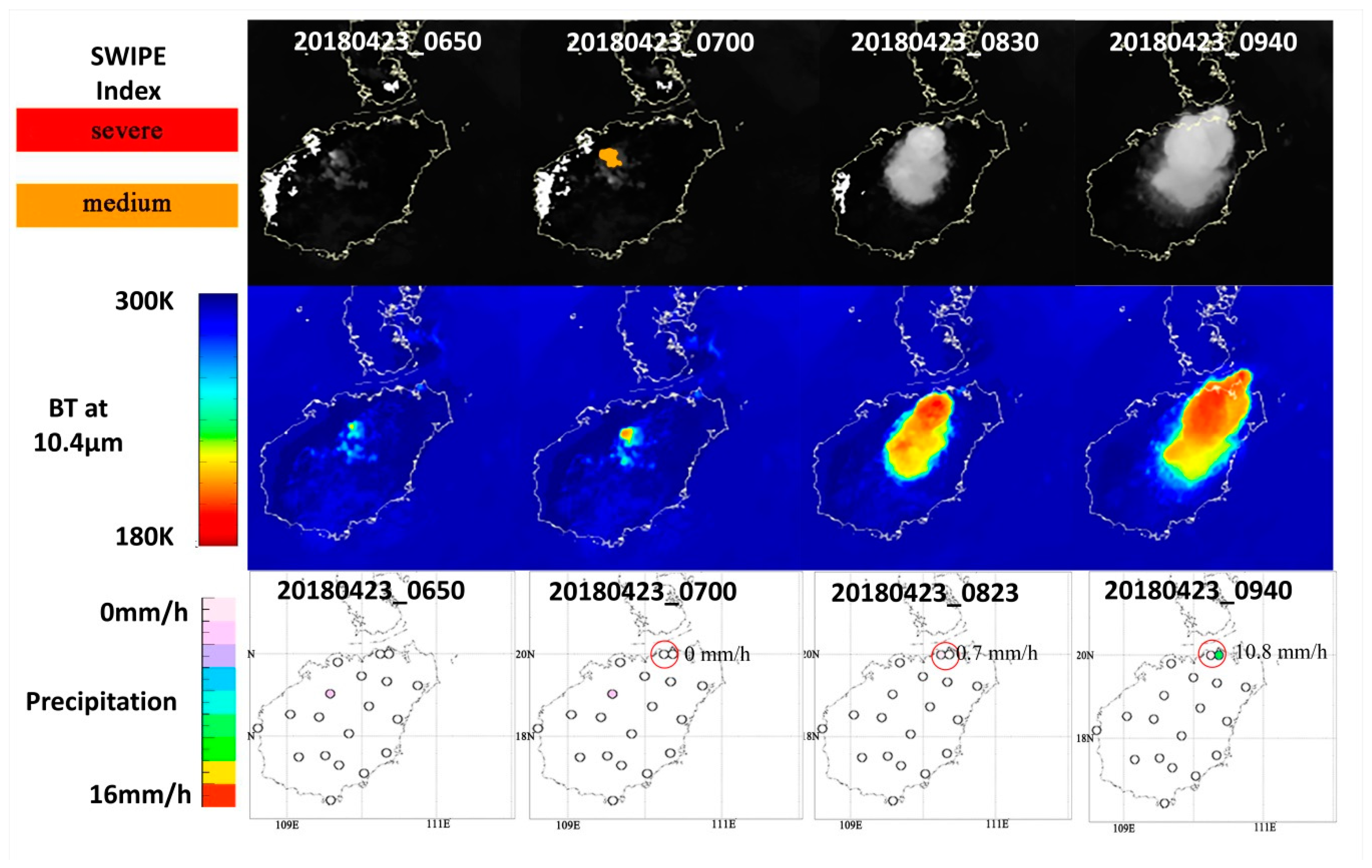
5.1. Case-1 at 07:00 UTC on 23 April 2018

The NRT SWIPE processing system successfully captured a medium sudden local convective storm case at 07:00 UTC (Beijing time 15:00) on 23 April 2018 in the Hainan province of China. This island is one of the southernmost islands of China with a mean latitude of 19°N, which has a typical tropical monsoon climate and tropical marine climate [33]. It is not surprising that this area often suffers from the attack of severe convective storm weather systems, in particular in the summertime. In addition, we also find many convective storm samples tracked by SWIPE from April to October in Figure 1. For precipitation, the ground station test results are the most accurate. The precipitation products are tested with the results of the ground test as the true value [16,38].

This convective storm case lasted about 3 hours. Its appearance and development is shown in Figure 5. From this figure, the SWIPE model initially marked a baby or newborn local convective storm system on the western side of Hainan Island at 07:00 UTC. This recognition result by the SWIPE algorithm disappeared immediately at 07:10 UTC (not shown here) due to the stable development of convective cloud cluster. According to the continuous records of the 21 ground-based rainfall gauge observations within 1 min intervals, the precipitation induced by this medium convective storm system initially occurs at 08:23 UTC in the Northern part of the island. In contrast, the H08/AHI can only take a picture for this convective storm system at 08:30 UTC. Therefore, the SWIPE model, in fact, captures this local sudden medium convective storm system one hour and twenty-three minutes earlier than the ground rainfall gauges (or radar). The sub-figures in the last column of Figure 5 exhibit the related results with the maximum rain rate of 10.8 mm/h at 09:40 UTC. It explicitly shows that the retrieved SWIPE index was two hours and 40 minutes earlier than the occurrence of the maximum rain rate.

5.2. Case-2 at 03:40 UTC on 27 July 2018

The NRT SWIPE model successfully captured another medium sudden convective storm case at 03:40 UTC (Beijing time 11:40) on 27 July 2018 in the Shandong province of China. As a typical North China Plain area, the average latitude of Shandong province is 35°N with moist summers and dry, cold winters (four distinct seasons). The summer precipitation generally contributes more than 50% of annual precipitation [48]. Since the precipitation area and the Intertropical Convergence Zone (ITCZ) have moved northward [49], Shandong Province will be frequently subjected to severe convective storm weather systems in the summer season (June, July, and August) as shown in Figure 1. The detailed process of this convection is shown in Figure 6.

This convective storm lasted about 2 hours. From the first row of Figure 6, it is found that the SWIPE model initially successfully captured a newborn sudden convective storm system in the central part of Shandong at 03:40 UTC. Note that, the continuous records of the 160 ground-based rainfall gauge data within 1-minute intervals in the Shandong province also clearly reveal that the rainfall first occurs at 03:51 UTC at the central part of Shandong Province. The sub-figures at the last column of Figure 6 exhibit the maximum rain rate of 51.3 mm/h (significantly larger than 16 mm/h) observed at 04:36 UTC. Therefore, in this case, the SWIPE model can capture sudden convective storm systems 56 minutes earlier than the occurrence of their maximum rain rate, whereas one hour ahead is completely adequate [50]. However, unfortunately, the SWIPE model underestimates the rank of this sudden convective storm system which should be a severe convection sample. This underestimation is likely to be induced by the relatively high FAR (0.91) of medium case using the Scenario-1 RF classification model.

6. Summary

This investigation aims to develop an efficient and robust predictive model called SWIPE for tracking and identifying sudden local convective storm systems over East Asia using combined AHI spectral, temporal, spatial information and the NWP based atmospheric environmental information. Based on an advanced RF learning algorithm, seven months of continuous GPM gridded rain rate data are used to define the three types of convective storms. H08/AHI and NWP data from April to October in 2016 are used to make a RF model training dataset. The RF algorithm is chosen because of its merits on better capturing non-linear patterns between predictors and sudden local convective storm systems. Before making a training dataset, a classical area-overlapped method is employed to track the potential convective cloud clusters using three continuous BT images at the 10.4 μm band from AHI. Built on the conclusions of previous studies, a sample-balance technique is used to randomly reduce the sample numbers of majority class in the training dataset. This technique can effectively equate the numbers of minority and majority class samples, and improve the poor performance on predicting both the minority and majority classes.

Finally, 83 variables in total, including IR window bands and water vapor absorption bands observations from H08/AHI, and the thermal (K-Index), dynamic (CAPE, CIN, LI, and EBS) and moisture (TPW) parameters of atmospheric environment from NWP, are chosen as predictors to train and establish the RF classification model. It is found that some variables from H08 (i.e. water vapor bands at 6.2 μm, 6.9 μm and 7.3 μm) and NWP data (i.e. TPW and CIN index) show relatively high ranks in RF model training. Because of their high dependency on convectively dominated precipitation areas, it implies the importance of predictors from both H08 and NWP data for training a convective storm system classification model.

Through parameter tuning iteratively in the RF model, an optimal classification predictive model is chosen here as final SWIPE for research and applications; which takes into account the needs for high POD on medium and severe convective storm systems recognition. The final accuracy of the optimal RF model under Scenario-1 is 0.79 for all the convective storm systems classification. The POD of the optimal RF model for severe and medium convections can also reach 0.66 and 0.70, respectively.

The use of NWP variables can noticeably improve the prediction of convective storms, especially for medium cases. Therefore, combined satellite and NWP data are important for the effective applications of this RF algorithm based SWIPE model. Two typical sudden local convective storm cases in Hainan and Shandong provinces of China in 2018 are studied for demonstration of SWIPE applications. These two cases are successfully tracked and captured by the SWIPE algorithm 2 hours and 40 minutes and 56 minutes earlier than the heavy rainfall event starting, respectively.

In the future, NWP data with a higher spatial resolution will be used to further improve the SWIPE prediction model. Also, some predictors for training SWIPE model need to be adjusted. While usually ground based radar observations provide critical information on storm development after it is initiated, in this study, the ground based radar observations are not used because the focus here is on the local convective storm identification in the pre-convection environment. The option to use ground-based radar observations will also be included in the model in the future. For example, the radar observations can be either used to define the convective categories instead of using GPM, or used as additional predictors in the RF model.

References

1. Taylor, C.M.; Belušić, D.; Guichard, F.; Parker, D.J.; Vischel, T.; Bock, O.; Harris, P.P.; Janicot, S.; Klein, C.; Panthou, G. Frequency of extreme Sahelian storms tripled since 1982 in satellite observations. Nature 2017, 544, 475–478. [Google Scholar] [CrossRef] [PubMed] [Green Version]
2. Proud, S.R. Analysis of aircraft flights near convective weather over Europe. Weather 2015, 70, 292–296. [Google Scholar] [CrossRef]
3. Zhang, Y.; Miao, S.; Dai, Y.; Bornstein, R. Numerical simulation of urban land surface effects on summer convective rainfall under different UHI intensity in Beijing. J. Geophys. Res. Atmos. 2017, 122. [Google Scholar] [CrossRef]
4. Mecikalski, J.R.; Mackenzie, W.M., Jr.; Koenig, M.; Muller, S. Cloud-Top Properties of Growing Cumulus prior to Convective Initiation as Measured by Meteosat Second Generation. Part I: Infrared Fields. J. Appl. Meteorol. Climatol. 2009, 49, 521–534. [Google Scholar] [CrossRef]
5. Weckwerth, T.M. Review of convection initiation and motivation for IHOP_2002. Mon. Weather Rev. 2006, 134, 5–22. [Google Scholar] [CrossRef]
6. Mecikalski, J.R.; Rosenfeld, D.; Manzato, A. Evaluation of Geostationary Satellite Observations and the Development of a 1–2 h Prediction Model for Future Storm Intensity. J. Geophys. Res. Atmos. 2016, 121. [Google Scholar] [CrossRef]
7. Mecikalski, J.R.; Bedka, K.M.; Paech, S.J.; Litten, L.A. A Statistical Evaluation of GOES Cloud-Top Properties for Nowcasting Convective Initiation. Mon. Weather Rev. 2010, 136, 4899–4914. [Google Scholar] [CrossRef]
8. Min, M.; Deng, J.; Liu, C.; Guo, J.; Lu, N.; Hu, X.; Chen, L.; Zhang, P.; Lu, Q.; Wang, L. An investigation of the implications of lunar illumination spectral changes for Day/Night Band-based cloud property retrieval due to lunar phase transition. J. Geophys. Res. Atmos. 2017, 122, 9233–9244. [Google Scholar] [CrossRef]
9. Ai, Y.; Li, J.; Shi, W.; Schmit, T.J.; Cao, C.; Li, W. Deep convective cloud characterizations from both broadband imager and hyperspectral infrared sounder measurements. J. Geophys. Res. Atmos. 2017, 122, 1700–1712. [Google Scholar] [CrossRef]
10. Maddox, R.A. Meoscale Convective Complexes. Bull. Am. Meteorol. Soc. 1980, 61, 469–475. [Google Scholar] [CrossRef]
11. Laing, A.G.; Carbone, R.E.; Levizzani, V. Cycles and Propagation of Deep Convection over Equatorial Africa. Mon. Weather Rev. 2010, 139, 2832–2853. [Google Scholar] [CrossRef]
12. Ai, Y.; Li, W.; Meng, Z.; Li, J. Life Cycle Characteristics of MCSs in Middle East China Tracked by Geostationary Satellite and Precipitation Estimates. Mon. Weather Rev. 2016, 144. [Google Scholar] [CrossRef]
13. Bedka, K.; Brunner, J.; Dworak, R.; Feltz, W.; Otkin, J.; Greenwald, T. Objective Satellite-Based Detection of Overshooting Tops Using Infrared Window Channel Brightness Temperature Gradients. J. Appl. Meteorol. Climatl. 2010, 49, 181–202. [Google Scholar] [CrossRef]
14. Wang, L. Cloud Classification of GMS-5 Data and Its Application in Rainfall Estimation. Sci. Atmos. Sin. 1998, 108, 1539–1543. [Google Scholar]
15. Thies, B.; Nauß, T.; Bendix, J. Precipitation process and rainfall intensity differentiation using Meteosat Second Generation Spinning Enhanced Visible and Infrared Imager data. J. Geophys. Res. Atmos. 2008, 113. [Google Scholar] [CrossRef] [Green Version]
16. Guo, J.; Deng, M.; Lee, S.S.; Wang, F.; Li, Z.; Zhai, P.; Liu, H.; Lv, W.; Yao, W.; Li, X. Delaying precipitation and lightning by air pollution over the Pearl River Delta. Part I: Observational analyses. J. Geophys. Res. Atmos. 2016, 121, 6472–6488. [Google Scholar] [CrossRef]
17. Ackerman, S.A. Global Satellite Observations of Negative Brightness Temperature Differences between 11 and 6.7 µm. J. Atmos. Sci. 1996, 53, 2803–2812. [Google Scholar] [CrossRef] [Green Version]
18. Shang, H.; Letu, H.; Nakajima, T.Y.; Wang, Z.; Ma, R.; Wang, T.; Lei, Y.; Ji, D.; Li, S.; Shi, J. Diurnal cycle and seasonal variation of cloud cover over the Tibetan Plateau as determined from Himawari-8 new-generation geostationary satellite data. Sci. Rep. 2018, 8. [Google Scholar] [CrossRef]
19. Schmit, T.J.; Li, J.; Gurka, J.J.; Goldberg, M.D.; Schrab, K.J.; Li, J.; Feltz, W.F. The GOES-R Advanced Baseline Imager and the Continuation of Current Sounder Products. J. Appl. Meteorol. Climatol. 2008, 47, 2696–2711. [Google Scholar] [CrossRef]
20. Min, M.; Chunqiang, W.U.; Chuan, L.I.; Liu, H.; Na, X.U.; Xiao, W.U.; Chen, L.; Wang, F.; Sun, F.; Qin, D. Developing the Science Product Algorithm Testbed for Chinese Next-Generation Geostationary Meteorological Satellites: Fengyun-4 Series. J. Meteorol. Res. 2017, 31, 708–719. [Google Scholar] [CrossRef]
21. Williams, J.K.; Ahijevych, D.A.; Kessinger, C.J.; Saxen, T.R.; Steiner, M.; Dettling, S. A machine learning approach to finding weather regimes and skillful predictor combinations for short-term storm forecasting. In Proceedings of the 13th Conference on Aviation, Range and Aerospace Meteorology, American Meteorological Society, New Orleans, LA, USA, 20–24 January 2008. [Google Scholar]
22. Min, M.; Bai, C.; Guo, J.; Sun, F.; Liu, C.; Wang, F.; Xu, H.; Tang, S.; Li, B.; Di, D.; et al. Estimating summertime precipitation from Himawari-8 and global forecast system based on machine learning. IEEE Trans. Geosci. Remote Sens. 2018. [Google Scholar] [CrossRef]
23. Karasiak, N. Remote Sensing of Distinctive Vegetation in Guiana Amazonian Park. In QGIS and Applications in Agriculture and Forest; Baghdadi, N., Mallet, C., Eds.; Wiley: Hoboken, NJ, USA, 2018; pp. 215–245. [Google Scholar]
24. Kühnlein, M.; Appelhans, T.; Thies, B.; Nauss, T. Precipitation estimates from MSG SEVIRI daytime, night-time and twilight data with random forests. J. Appl. Meteorol. Climatol. 2014, 53, 2457–2480. [Google Scholar] [CrossRef]
25. Li, J.; Li, J.; Otkin, J.; Schmit, T.J.; Liu, C.Y. Warning information in a preconvection environment from the geostationary advanced infrared sounding system—A simulation study using the IHOP case. J. Appl. Meteorol. Climatol. 2011, 50, 776–783. [Google Scholar] [CrossRef]
26. Min, M.; Zhang, Z. On the influence of cloud fraction diurnal cycle and sub-grid cloud optical thickness variability on all-sky direct aerosol radiative forcing. J. Quant. Spectr. Radiat. Transf. 2014, 142, 25–36. [Google Scholar] [CrossRef] [Green Version]
27. Min, M.; Wang, P.; Campbell, J.R.; Zong, X.; Li, Y. Midlatitude cirrus cloud radiative forcing over China. J. Geophys. Res. Atmos. 2010, 115. [Google Scholar] [CrossRef] [Green Version]
28. Roman, J.; Knuteson, R.; Ackerman, S.; Revercomb, H. Estimating minimum detection times for satellite remote sensing of trends in mean and extreme precipitable water vapor. J. Clim. 2016, 29. [Google Scholar] [CrossRef]
29. Huffman, G.J.; Bolvin, D.T.; Braithwaite, D.; Hsu, K.; Joyce, R.; Kidd, C.; Nelkin, E.J.; Sorooshian, S.; Tan, J.; Xie, P. Algorithm Theoretical Basis Document (ATBD) Version 5.2: NASA Global Precipitation Measurement (GPM) Integrated Multi-SatellitE Retrievals for GPM (IMERG). NASA: Greenbelt, MD, USA, 2018. Available online: http://pmm.nasa.gov/sites/default/files/document_files/IMERG_ATBD_V5.2.pdf (accessed on 13 February 2019).
30. Tang, G.; Zeng, Z.; Long, D.; Guo, X.; Yong, B.; Zhang, W.; Hong, Y. Statistical and hydrological comparisons between TRMM and GPM level-3 products over a midlatitude basin: Is day-1 IMERG a good successor for TMPA 3B42V7? J. Hydrometeorol. 2015, 17. [Google Scholar] [CrossRef]
31. Huffman, G.J.; Adler, R.F.; Bolvin, D.T.; Nelkin, E.J. The TRMM Multi-Satellite Precipitation Analysis (TMPA). Satell. Appl. Surface Hydrol. 2010, 9, 3–22. [Google Scholar]
32. Yihui, D.; Chan, J.C.L. The East Asian summer monsoon: An overview. Meteorol. Atmos. Phys. 2005, 89, 117–142. [Google Scholar] [CrossRef]
33. Yun, K.S.; Lee, J.Y.; Ha, K.J. Recent intensification of the South and East Asian monsoon contrast associated with an increase in the zonal tropical SST gradient. J. Geophys. Res. Atmos. 2014, 119, 8104–8116. [Google Scholar] [CrossRef] [Green Version]
34. Glickman, T.S. Glossary of Meteorology; American Meteorological Society: Boston, MA, USA, 2000. [Google Scholar]
35. Morel, C.; Sénési, S.; Autones, F. Building Upon Saf-Nwc Products: Use of the Rapid Developing Thunderstorms (Rdt) Product In MÉTÉO-France Nowcasting Tools. Meteorol. Satell. Data Users’ Conf. 2002, 248–255. [Google Scholar]
36. Sieglaff, J.M.; Cronce, L.M.; Feltz, W.F.; Bedka, K.M.; Pavolonis, M.J.; Heidinger, A.K. Nowcasting convective storm initiation using satellite-based box-averaged cloud-top cooling and cloud-type trends. J. Appl. Meteorol. Climatol. 2011, 50, 110–126. [Google Scholar] [CrossRef]
37. Stensrud, D.J.; Fritsch, J.M. Mesoscale convective systems in weakly forced large-scale environments. part ii: Generation of a mesoscale initial condition. Mon. Weather Rev. 1994, 122, 2068–2083. [Google Scholar] [CrossRef]
38. Guo, J.; Su, T.; Li, Z.; Miao, Y.; Li, J.; Liu, H.; Xu, H.; Cribb, M.; Zhai, P. Declining frequency of summertime local-scale precipitation over eastern China from 1970 to 2010 and its potential link to aerosols. Geophys. Res. Lett. 2017, 44. [Google Scholar] [CrossRef]
39. Breiman, L. Random Forests. Mach. Learn. 2001, 45, 5–32. [Google Scholar] [CrossRef] [Green Version]
40. Ramirez, S.; Lizarazo, I. Detecting and tracking mesoscale precipitating objects using machine learning algorithms. Int. J. Remote Sens. 2017, 38, 5045–5068. [Google Scholar] [CrossRef]
41. Pavolonis, M.J.; Feltz, W.F.; Heidinger, A.K.; Gallina, G.M. A daytime complement to the reverse absorption technique for improved automated detection of volcanic ash. J. Atmos. Ocean. Technol. 2006, 23, 1422–1444. [Google Scholar] [CrossRef]
42. Reed, R.J.; Hollingsworth, A.; Heckley, W.A.; Delsol, F. An Evaluation of the Performance of the ECMWF Operational System in Analyzing and Forecasting Easterly Wave Disturbances over Africa and the Tropical Atlantic. Mon. Weather Rev. 2009, 116, 824–865. [Google Scholar]
43. Laing, A.G.; Fritsch, J.M. The Large-Scale Environments of the Global Populations of Mesoscale Convective Complexes. Mon. Weather Rev. 2000, 128, 2756–2776. [Google Scholar] [CrossRef]
44. Zhang, G.J. Roles of tropospheric and boundary layer forcing in the diurnal cycle of convection in the U.S. southern great plains. Geophys. Res. Lett. 2003, 30, 665–678. [Google Scholar] [CrossRef]
45. Liu, Y.; Chawla, N.V.; Harper, M.P.; Shriberg, E.; Stolcke, A. A study in machine learning from imbalanced data for sentence boundary detection in speech. Comput. Speech Lang. 2006, 20, 468–494. [Google Scholar] [CrossRef]
46. Tahir, M.A.; Kittler, J.; Yan, F. Inverse random under sampling for class imbalance problem and its application to multi-label classification. Pattern Recognit. 2012, 45, 3738–3750. [Google Scholar] [CrossRef]
47. Wilks, D.S. Statistical Methods in the Atmospheric Sciences. In International Geophysics, 2nd ed.; Academic Press: Cambridge, MA, USA, 2005; p. 91. [Google Scholar]
48. Fu, G.B.; Charles, S.P.; Yu, J.J.; Liu, C.M. Decadal climatic variability, trends, and future scenarios for the north China plain. J. Clim. 2009, 22, 2111–2123. [Google Scholar] [CrossRef]
49. Guo, J.; Liu, H.; Li, Z.; Rosenfeld, D.; Jiang, M.; Xu, W.; Jiang, J.; He, J.; Chen, D.; Min, M.; et al. Aerosol-induced changes in the vertical structure of precipitation: A perspective of TRMM precipitation radar. Atmos. Chem. Phys. 2018, 18, 13329–13343. [Google Scholar] [CrossRef]
50. Sun, J.; Chen, M.; Wang, Y. A frequent-updating analysis system based on radar, surface, and mesoscale model data for the Beijing 2008 forecast demonstration project. Weather Forecast. 2010, 25, 4236–4248. [Google Scholar] [CrossRef]
Figure 1. Spatial distributions of three typical convective storm systems from April to October of 2016. Gray, orange, and red solid circles respectively represent slight (or none), medium, and severe convective storm systems.
Remotesensing 11 00383 g001
Figure 2. A real case of tracked convective storm system at 19:30 UTC on 05 July 2016 in Guangdong province of China based on H08/AHI observations. The first small sub-figure at the upper-left corner is the grayscale 10.4 μm BT image with coast line (yellow solid line). The other three small colorful sub-figures at the left panel represent 10.4 μm BT images at 19:10, 19:20, and 19:30 UTC, respectively. The colorful area in right panel represents the pixels of H08/AHI with BT<238 K at 19:30 UTC on 05 July 2016.
Remotesensing 11 00383 g002
Figure 3. The flow chart of SWIPE model training and predicting based on RF algorithm. It contains three steps: First, it tracks potential convective cloud clusters. The second step is to divide the convective storm system dataset into three different types (weak, medium, and severe). Finally, the RF algorithm is used to train and develop a convection intensity classification statistical model — SWIPE. Δ T represents the cloud top cooling rate.
Remotesensing 11 00383 g003
Figure 4. Effects of total number of trees in the forest (n_estimators), maximum depth of the tree (max_depth), and random split predictor variables (max_features = 7 (upper left), 8 (upper right), 9 (middle left), 10 (middle right), and 11 (lower left)) on OOB scores for the RF classification models of convective storm system.
Remotesensing 11 00383 g004
Figure 5. A sudden convective storm case tracked by the SWIPE model at 07:00 UTC on 23 April 2018 in the Hainan province of China. The sub-figures in the first row represent the results of SWIPE index and the grayscale 10.4 μm BT image with coast line (yellow solid line). The colorful sub-figures at the second row represent the 10.4 μm BT images. The sub-figures in the third row are the accumulated precipitation in the past one hour (mm/h) measured by the ground rainfall gauge stations. The sub-figures in the first and second columns signify the two contiguous results or scenarios when this convective storm case in Hainan province is tracked by the SWIPE model at the first time. The sub-figures in the third and fourth columns represent the results or scenarios with the first rainfall measurement and the maximum rain rate, respectively.
Remotesensing 11 00383 g005
Figure 6. Same as Figure 5, for a sudden convective storm case at 03:40 UTC on 27 July 2018 in Shandong province of China.
Remotesensing 11 00383 g006