Object Detection in Remote Sensing Images Based on a Scene-Contextual Feature Pyramid Network

Key Lab of Optoelectronic Technology & Systems of Education Ministry, Chongqing University, Chongqing 400044, China
*
Author to whom correspondence should be addressed.
Remote Sens. 2019, 11(3), 339; https://doi.org/10.3390/rs11030339
Submission received: 14 January 2019
/
Revised: 31 January 2019
/
Accepted: 6 February 2019
/
Published: 8 February 2019
Abstract
:Object detection has attracted increasing attention in the field of remote sensing image analysis. Complex backgrounds, vertical views, and variations in target kind and size in remote sensing images make object detection a challenging task. In this work, considering that the types of objects are often closely related to the scene in which they are located, we propose a convolutional neural network (CNN) by combining scene-contextual information for object detection. Specifically, we put forward the scene-contextual feature pyramid network (SCFPN), which aims to strengthen the relationship between the target and the scene and solve problems resulting from variations in target size. Additionally, to improve the capability of feature extraction, the network is constructed by repeating a building aggregated residual block. This block increases the receptive field, which can extract richer information for targets and achieve excellent performance with respect to small object detection. Moreover, to improve the proposed model performance, we use group normalization, which divides the channels into groups and computes the mean and variance for normalization within each group, to solve the limitation of the batch normalization. The proposed method is validated on a public and challenging dataset. The experimental results demonstrate that our proposed method outperforms other state-of-the-art object detection models.
1. Introduction
Object detection in remote sensing images is of great importance for many practical applications, such as urban planning and urban ecological environment evaluation. Recently, due to the powerful feature extraction ability in convolutional neural networks (CNNs), the deep learning methods [1,2,3,4,5,6,7,8] have achieved great success in object detection. Region-based CNN (R-CNN) [9] is one of the earliest algorithms employing CNN, and it has been shown to have a great and positive impact on object detection. In R-CNN, the regions that possibly contain the target objects, which are called “regions of interest” (ROIs), are generated by a selective search algorithm (SS algorithm) [10]. Then, with a CNN algorithm, the R-CNN locates the target objects in the ROIs. Following R-CNN, many other related models have been proposed. Fast R-CNN [11] and faster R-CNN [12] are two of the representative related methods. In fast R-CNN, the model maps all the ROIs onto a feature map of the last convolutional layer so that it can extract the features of an entire image at one time and greatly shorten the running time. In faster R-CNN, the model develops a region proposal network (RPN) to replace the original SS algorithm to optimize the ROI generation method. The RPN takes an arbitrary scale image as the input and produces a series of rectangular ROIs, assigning each of the output ROIs with an objectivity score. Thus, with the objectivity scores, the faster R-CNN model can filter out many low-scoring ROIs and shorten the detection time. Although these methods have achieved good results in object detection, both of them still adopt a single-scale feature layer in which the detection of targets with various scales, especially small-sized objects, is not effective.
Therefore, research on object detection based on multi-scale features has become the mainstream topic of current research [13]. In the early stages of this research, researchers used image pyramids to construct multi-scale features, i.e., image scales of different sizes to generate corresponding features and achieve multi-scale features. However, image scaling increases the amount of time required for analysis. The single shot multibox detector (SSD) algorithm [14] improves the image pyramid method and achieves multi-scale feature by fusing different scale features from different layers that do not add extra computation. However, in the SSD algorithm, low-level features, which are effective for small object detection, are not fully utilized. A feature pyramid network (FPN) [15] adopts a top-down and bottom-up structure that makes full use of the low-level and high-level features, requires no additional computation, and has an excellent detection effect, especially for small objects.
Due to the great breakthrough and rapid development of object detection in natural images, researchers in the field of remote sensing image processing have paid increased attention to CNN-based object detection methods. However, compared with natural images, CNN-based detection methods have several limitations:
In light of the above problems, researchers have put forward several solutions. Vakalopoulou et al. [16] proposed an automatic building detection model, which was based on deep convolutional neural network theory, was trained by a huge dataset using supervised learning, and was capable of effectively realizing the accurate extraction of irregular buildings. Ammour et al. [17] used a deep convolutional neural network system for car detection in unmanned aerial vehicle (UAV) images. In their method, the system first segmented the input image into small homogeneous regions and then used a deep CNN model combined with a linear support vector machine (SVM) classifier to classify “car” regions and “non-car” regions. Zhang et al. [18] extracted the features of an object by training a CNN model. Combined with a modified ellipse, a line segment detector (for select candidates in the images), and a histogram of oriented gradients (HOG) feature (for classification), their model obtained good performance in different complex backgrounds. Long et al. [19] used a CNN-based model for object detection and proposed an unsupervised score-based bounding box regression algorithm for pruning the bounding boxes of regions (after classification), ultimately improving the accuracy of object localization. Zhang et al. [20] built a weakly supervised iterative learning framework to augment the original training image data. The proposed framework was effective in solving the problem of lacking samples for training and obtained good performance with respect to aircraft detection. To solve the problem of not having enough samples for training, Maggiori et al. [21] used a two-step training approach for recognizing remote sensing images; they first initialized a CNN model by using a large amount of possibly inaccurate reference data and then refined a small amount of accurately labeled data. In this way, their model also effectively solves the problem of the lack of data. Sun et al. [22] presented a novel two-level training CNN model, which consisted of a CNN model for detecting the location of cities in remote sensing images and a CNN model for the further detection of multi-sized buildings. Cheng et al. [23] proposed a rotation of invariant deep CNN models. The model designed a novel layer of networks for extracting the features of oriented objects and effectively solved the orientation detection problem. Chen et al. [24] also focused on the problem of object orientation, but approached it differently than Cheng et al., by proposing an orientation CNN model to detect the direction of buildings and using an oriented bounding box for improving the location and accuracy of building detection. In recent years, the target detection task in remote sensing images based on multi-scale feature framework has also been attracting more and more attention from researchers. Deng et al. [25] designed a multi-scale feature framework by constructing a multiple feature map with multiple filter sizes and achieved effective detection of small targets. Similarly, Guo et al. [26] proposed an optimized object proposal network to produce multiple object proposals. The method adds multi-scale anchor boxes to multi-scale feature maps for which the network can generate object proposals exhaustively, which improve the performance of the detection. In addition to focusing on multiple size object detection, Yang et al. [27] also considered the rotation of the target, proposing a framework called a rotation dense feature pyramid network (R-DFPN) that can effectively detect ships in different scenes, including oceans and ports. Yu et al. [28] proposed an end-to-end feature pyramid network (FPN)-based framework that is effective for multiple ground object segmentation.
In our work, we analyze the relationships between objects and scenes in remote sensing images. Specifically, we analyze the training part of a large-scale dataset for object detection in aerial images: DOTA dataset [29] by counting the number of images of each class of object and the number of images in which the object appears in relevant scenes. As shown in Table 1, we found that most of the objects appear in their relevant scenes in remote sensing images and that the objects have a strong correlation with the contextual information of their scene.
Therefore, in this paper, we propose a multi-scale CNN-based detection method called a scene-contextual feature pyramid network (SCFPN), which is based on an FPN, by combining scene-contextual features with a backbone network. There have been some similar methods to ours. However, different from the FPN, the proposed method fully considers the context of the scene and improves the backbone network structure. The main contributions of this paper are as follows:
- We propose the scene-contextual feature pyramid network, which is based on a multi-scale detection framework, to enhance the relationship between scene and target and ensure the effectiveness of the detection of multi-scale objects.
- We apply a combination structure called ResNeXt-d as the block structure of the backbone network, which can increase the receptive field and extract richer information for small targets.
- We use the group normalization layer into the backbone network, which divides the channels into groups and computes within each group the mean and the variance for normalization, to solve the limitation of the batch normalization layer, and eventually get a better performance.
Experiments based on remote sensing images from a public and challenging dataset for object detection show that the detection method based on the proposed SCFPN demonstrates state-of-the-art performance. The rest of this paper is organized as follows: Section 2 introduces the details of the proposed method. Section 3 presents the experiments conducted on the remote sensing dataset to validate the effectiveness of the proposed method. Section 4 discusses the results of the proposed method. Finally, Section 5 concludes the paper.
2. Proposed Method
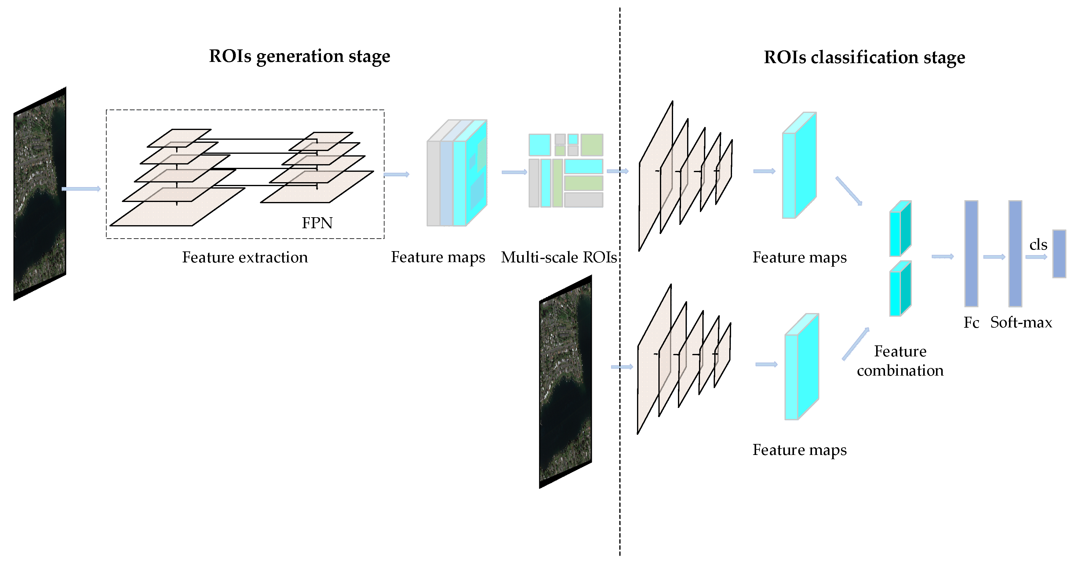
In this section, we will detail the various parts of the proposed SCFPN framework. Figure 1 shows the overall framework of the proposed SCFPN. The framework mainly consists of two parts: an RPN based on a feature pyramid network (FPN-RPN) for multi-scale ROI generation and a scene-contextual feature fusion network for ROI classification. Specifically, in the FPN-RPN, we first generated feature maps that are fused by multi-scale features for each input image. Then, we generated multi-scale ROIs by using the FPN-RPN. In scene-contextual feature fusion network, we first extracted the features of the scene context and generated multi-scale ROIs by using the backbone network. Then, we fused the features by combining them in order to train a classifier. Finally, the class prediction of the ROIs were processed with the classifier.
2.1. SCFPN Framework
The proposed SCFPN detection framework is based on faster FPN [15], which makes full use of low-level and high-level features and can detect multi-sized objects effectively. These advantages are suitable for the task of object detection in remote sensing images, which have a wide range of sizes of targets. Similar to faster FPN, we adopted a two-stage detection framework, which has a ROI generation stage and a ROI classification stage.
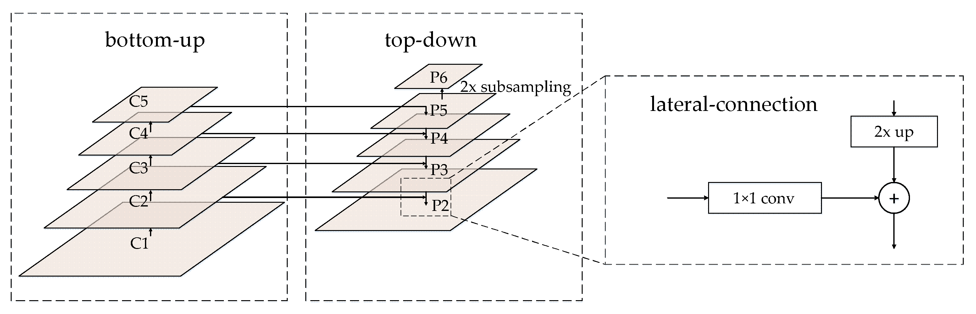
In the ROI generation stage, we constructed a multi-scale RPN network based on an FPN framework, which is called FPN-RPN. Figure 2 shows the structure of the FPN-RPN. The FPN-RPN consisted of three parts: the bottom-up feedforward network, top-down network, and lateral connections. In the bottom-up feedforward network, we chose the multilevel feature maps {, , , }, corresponding to the output of the last layer of each network stage, which had the strongest semantic features. All of them had strides of {4, 8, 16, 32} pixels relative to the input image. In the top-down network, we strengthened the high-level features by up-sampling the lateral connections to the previous feature {, , , } and achieving higher resolution features {, , , }. Specifically, in the lateral connection, we first performed 2× up-sampling by using the nearest-neighbor up-sampling method on the high-level feature map (); then, we combined it with the corresponding preceding feature map () and achieved a new feature map (). Finally, we repeated this process until the finest feature map () was generated. It should be noted that, in order to maintain the same number of channels in the preceding and subsequent feature maps, the preceding map needs to be processed by a 11 convolutional kernel. In the anchor setting, to cover a larger anchor scale of , we introduced , which is simply a stride 2 subsampling of . {, , , , } correspond to the anchor scales of {, , , , }, respectively.
Moreover, we designed a scene-contextual feature fusion network for ROI classification, which is different from the faster FPN, which directly inputs the generated ROI feature maps into the backbone network for classification. In our proposed scene-contextual feature fusion network, we construct two feature extraction branches, which use the same backbone architecture to extract the global image feature and ROI features, respectively. Specifically, we first extracted the global image feature and the multi-scale ROI features using the backbone network. To solve the problem of the mismatch of the size of the features, the ROI align pooling layer [30] was used to resize the multi-scale ROI features and the global image feature to the same size and achieve the resized multi-scale ROIs feature and global feature . Then, we combined and into a fusion feature . The fusion feature are defined as follows:
Finally, we input the fusion features of the ROIs into the soft-max classifier for predicting the class of each ROI and achieving the final detection results.
To train the proposed SCFPN model, we used a multi-task loss function [11], which is defined as follows:
where j is the index of an anchor in a mini-batch, is the predicted probability of anchor j being an object region, and is the ground-truth label, which is 0 for negative and 1 for positive. The predicted box and the ground-truth box are defined in [11]. The two terms and in Equation (2) are normalized with ,, and a balancing weight , respectively. In addition, the function of smoothL1 [11] is defined as follows:
2.2. Backbone Network
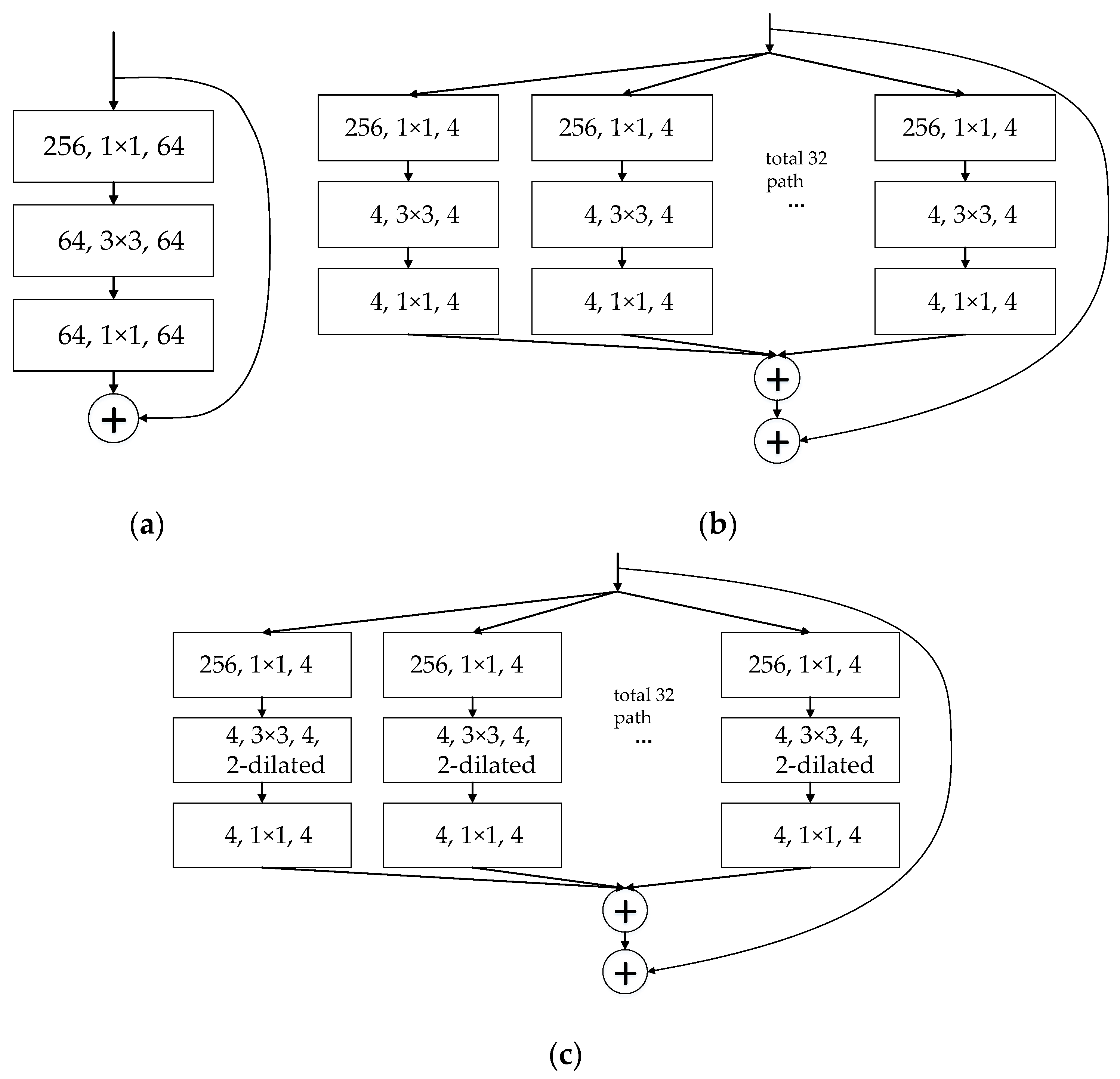
Traditionally, to improve the performance and feature extraction capability of the backbone network, the network is always deepened or widened. However, with the increase of the number of hyper-parameters (such as channels, filter size, etc.), the difficulty of network training and computational overhead increases. Thus, ResNeXt [31], which adopts the aggregated residual transform block structure as the backbone network to improve the performance without increasing the complexity of the parameters while reducing the number of hyper-parameters, was utilized. However, the model still faces the problem that a naive subsampling inadvertently loses the details in the feature map rescaling. Dilated convolution [32] is one of the variants of convolution. Compared with convolution, the dilated convolution filter has a dilation rate for representing the size of the receptive field dilation. The larger the dilation rate, the larger the receptive field, corresponding to the convolution kernel size. This improvement of convolution obtains a greater receptive field, which can solve the problem of losing details when subsampling the feature map. Therefore, we applied the block of ResNeXt and introduced a dilated convolutional filter to obtain a combination structure called ResNeXt-d, which enlarges the receptive field and enhance the perception of small targets.
Figure 3 shows three kinds of structures of blocks: (a) a block of ResNet [33]; (b) a block of ResNeXt; and (c) a block of the proposed method. Figure 3 shows that the block of ResNeXt (Figure 3b) divides the original residual block (Figure 1a) into branches by width, each of which is called a cardinality. Specifically, Figure 3b shows a block of ResNeXt with a cardinality = 32. The proposed block of ResNeXt-d is shown in Figure 3c. The main difference between the proposed block of ResNeXt-d (Figure 3c) and the block of ResNeXt (Figure 3b) is that the middle 33 convolutional filter is replaced by a 33 dilated convolutional filter with a dilatation rate of 2 (denoted by the term “2-dilated” in Figure 3c).
The proposed backbone network consists of a stack of residual blocks. These blocks have the same topology and are subject to the same simple rules as ResNeXt/ResNet. Table 1 shows the structure of 50 layers of the ResNet, ResNeXt, and ResNeXt-d backbone networks. Convolutional layer parameters in the ResNet, ResNeXt, and ResNeXt-d networks are denoted as “filter size, number of channel”, “filter size, number of channel, number of cardinality”, and “filter size, dilation rate, number of channel, number of cardinality”, respectively. In the Table 1, we can see that in the backbone of the proposed method, we divide the block of ResNet into 32 branches by width (set cardinality = 32) and replace the middle 33 convolutional filter with a 33 dilated convolutional filter with a dilatation rate of 2 (set dilatation rate = 2), which enlarges the receptive field into 77 and makes the convolution output contain richer information of targets, especially of small targets. In addition, the parameter scales, the total number of parameters of all the layers, of the three models are similar (last row in Table 2).
2.3. Group Normalization
Batch normalization (BN) [34] is commonly used in deep learning and has a significant effect on improving training and the convergence speed. In BN, the normalization calculation is based on the dimension of the batch, and this leads to a strong dependence on the setting of the batch size. Generally, setting a larger batch size is more suitable for training and can achieve better performance. However, with respect to object detection in remote sensing images, because of the large size of the input images, the batch size can only be set to 2 or 4 with an 11-Gigabyte random access memory, graphic processing unit (11-GB RAM GPU), which greatly limits the performance of the model. To solve this problem, we used group normalization (GN) [35], which cleverly avoids the batch size limitation to achieve object detection in remote sensing images.
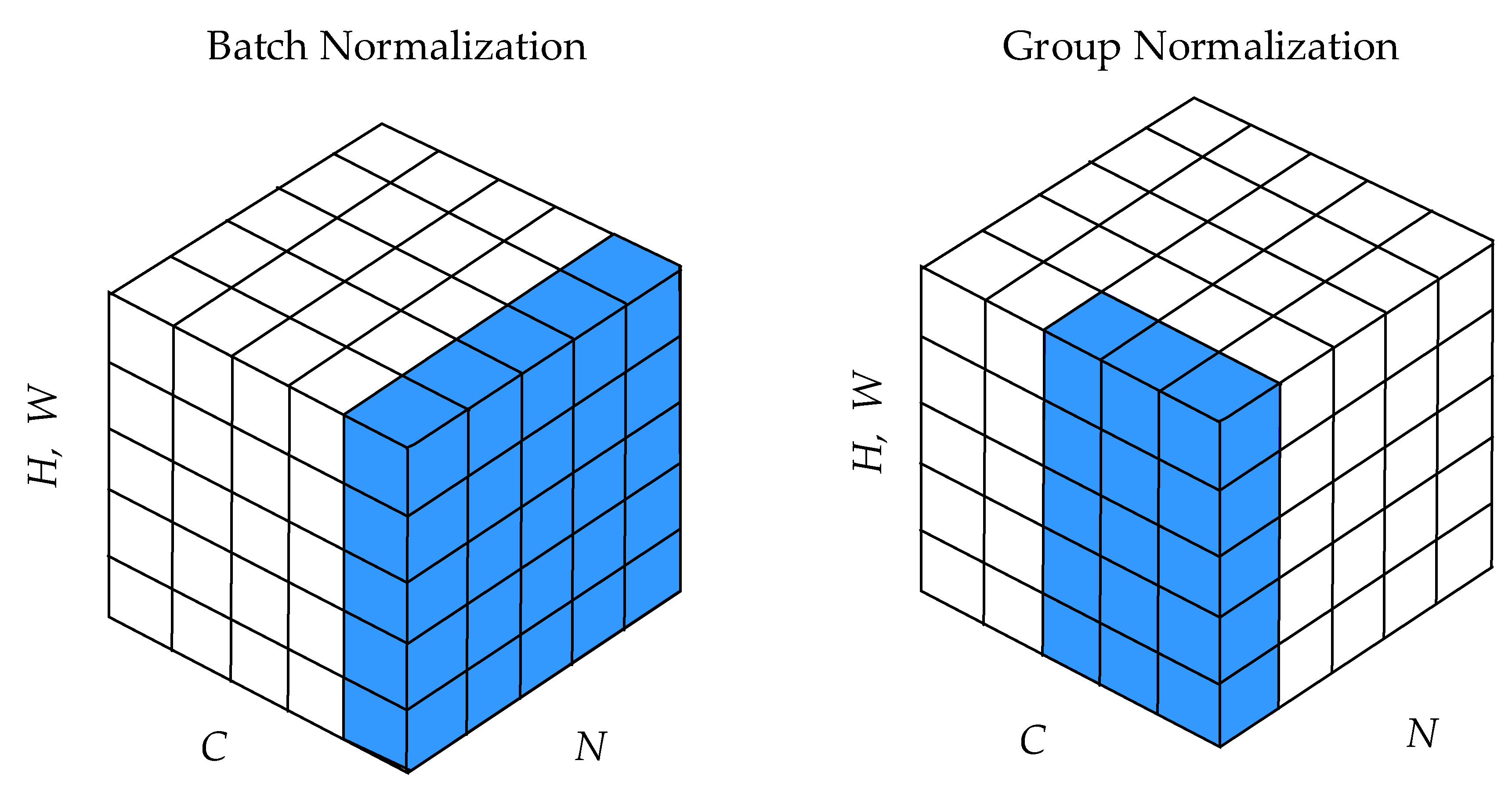
In the case of remote sensing images, the data in the deep network is in a four-dimensional (4D) vector (N, C, H, W) order, where N is the batch axis, C is the channel axis, and H and W are the spatial height and width axes. Figure 4 shows how BN and GN calculate the mean and variance, respectively. It notes that each small cube denotes a pixel and the pixels in blue are normalized by the same mean and variance, computed by aggregating the values of these pixels. As shown in Figure 4, BN is normalized in the batch direction; for each channel, it computes the mean and variance along the (NHW) axes. Therefore, the larger the size of N, the more accurate the mean and variance of the calculation. GN divides the channels into groups and computes within each group index i the mean and variance for normalization. Formally, a GN layer computes the mean and variance in a set of pixels , defined as follows [34]:
where G is the number of groups, which is a pre-defined hyper-parameter (we set G = 64 for our model); C/G is the number of channels per group; is the floor operation; and and denote the sub-index of i and k along the N axis. This means that the pixels sharing the same batch index are normalized together. Additionally, and denote the sub-index of i and k along the C axis and “” denotes that the indexes i and k are in the same group of channels, assuming each group of channels is stored in a sequential order along the C axis. Thus, GN computes the mean and variance only along the (H, W) axes and along group channels, and this effectively avoids the limitation of the batch size in the training model. Through a large number of experimental comparisons, we found that the use of GN can significantly improve the detection performance while keeping the computation consumption at a low level.
3. Experiments
To evaluate the performance of the proposed SCFPN, we performed the 15-class object detection experiments on a publicly available and challenging dataset: the DOTA dataset [29]. The dataset description, evaluation metrics, and training details are described in this section.
3.1. Dataset Description
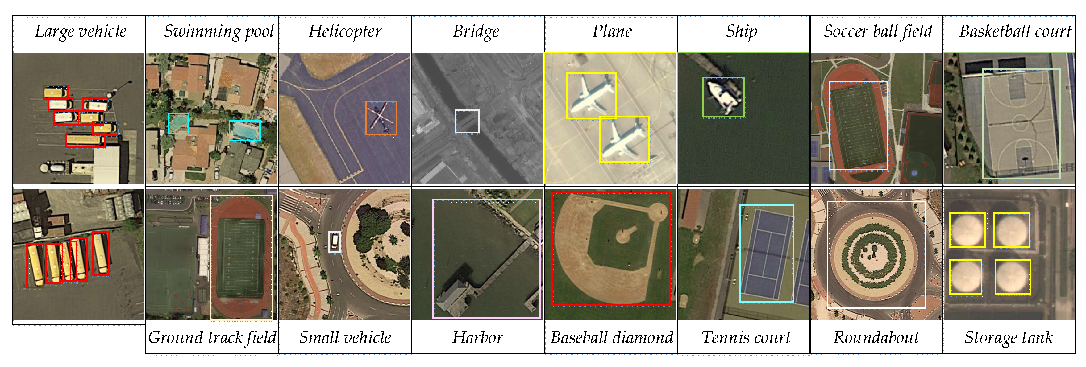
The DOTA dataset is a 15-class geospatial object detection dataset for multi-class object detection. This dataset contains the following classes of objects: soccer ball field, helicopter, swimming pool, roundabout, large vehicle, small vehicle, bridge, harbor, ground track field, basketball court, tennis court, baseball diamond, storage tank, ship, and plane. It collates a total of 2806 aerial images, and the sizes of the images range from about 800 × 800 to about 4000 × 4000. Various pixel sizes of objects are considered in the dataset. It labels a total of 188,282 instances: 57% of them are small object instances ranging from 10 pixels to 50 pixels; 41% are middle object instances ranging from 50 pixels to 300 pixels; and 2% are large objects of over 300 pixels. In order to ensure that the training data and test data distributions approximately match, the dataset randomly selects 1/2 as a training set, 1/6 as a validation set, and 1/3 as the testing set. Figure 5 shows the samples of the dataset.
3.2. Evaluation Metrics
In this paper, we utilized the widely used average precision (AP) [22,23,24], precision-recall curve (PRC) [25,26,27], and F-measure (F1) [25,27,36] metrics to quantitatively evaluate the performance of the proposed SCFPN. The AP computes the average value of the precision over the interval from recall = 0 to recall = 1, and the higher the AP, the better the performance. Additionally, the mean AP (mAP) computes the average precision of all classes. The precision metric measures the fraction of detections that are true positives; the recall metric measures the fraction of positives that are correctly identified. The F1 metric combines the precision and recall metrics into a single measure to comprehensively evaluate the quality of an object detection method. The precision, recall, and F1 metrics can be formulated as follows:
where TP denotes the number of true positives, TN denotes the number of true negatives, FP denotes the number of false positives, and FN denotes the number of false negatives. It is worth mentioning that the judgment of true positives or false positive in a detection task is dependent on the widely used Intersection-Over-Union (IOU) metric. If the value of IOU is greater than or equal to 0.7, the region is treated as a true positive; otherwise, it is a false positive.
3.3. Training Details
Following training strategies were provided by the Detectron [37] repository. Our proposed detectors are end-to-end trained on a Nvidia GTX 1080Ti GPU with 11-GB RAM and are optimized by synchronized stochastic gradient descent (SGD) [12] with a weight decay of 0.0001 and momentum of 0.9. Each mini-batch has 2 images, and we resized the shorter edge of the image to 800 pixels; the longer edge is limited to 1333 pixels to avoid using too much memory. We trained a total of 140,000 iterations, with a learning rate of 0.001 for the first 100,000 iterations, 0.0001 for the next 20,000 iterations, and 0.00001 for the remaining 20,000 iterations.
All the experiments were initialized with common objects in context (COCO) pre-trained weights. Group normalization was fixed during the detector fine-tuning. We only adopted a simple horizontal image flipping data augmentation. As for ROI generation, we first picked up 10,000 proposals with the highest scores and then used a non-maximum suppression (NMS) operation to get, at most, 2000 ROIs for training. In testing, we took 2000/10,000 (10,000 highest scores for NMS, 2000 ROIs after NMS) for the setting. We also used the popular and effective ROI-Align [30] technique in the proposed model.
4. Results and Discussion
4.1. Results
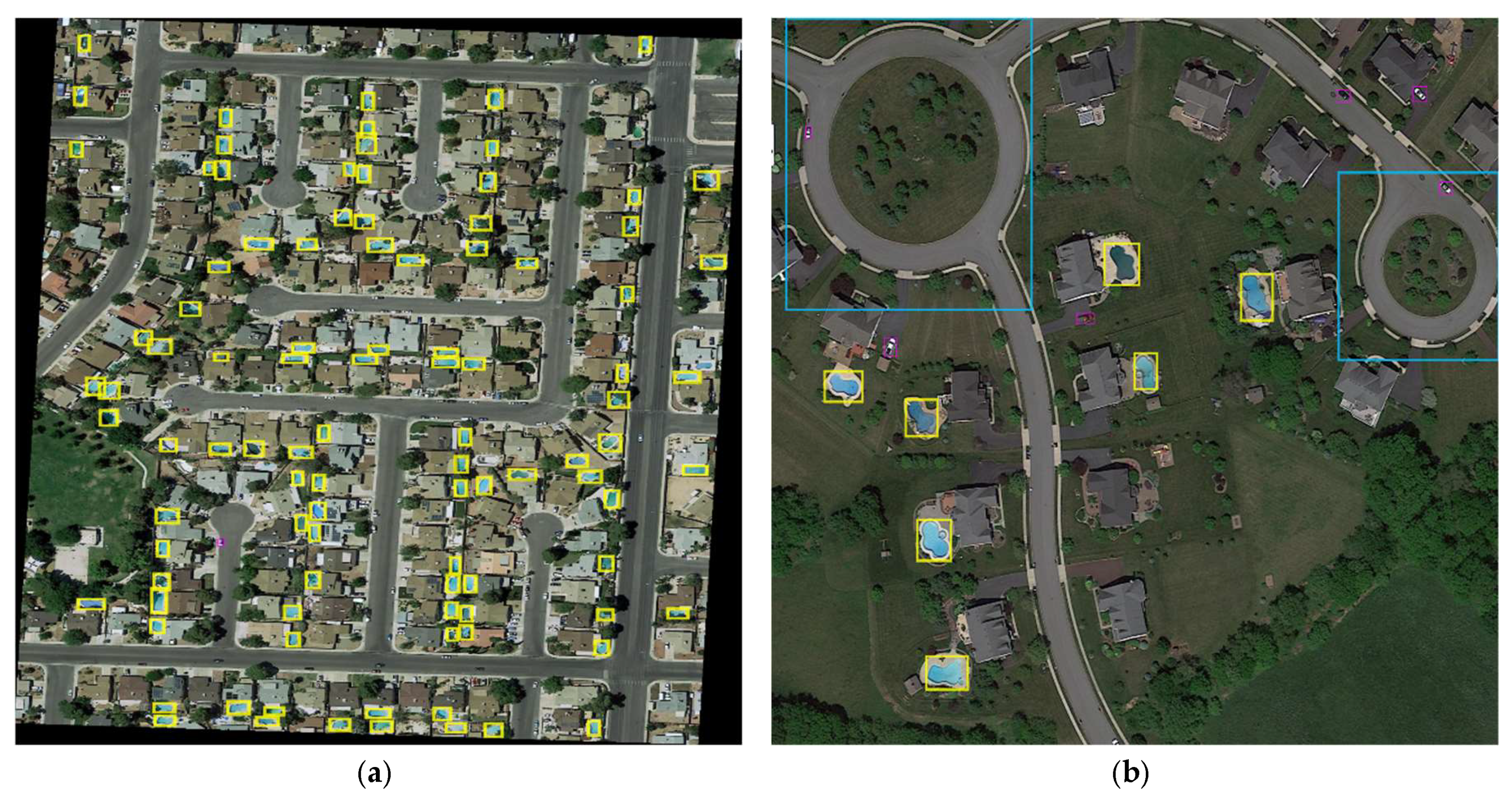
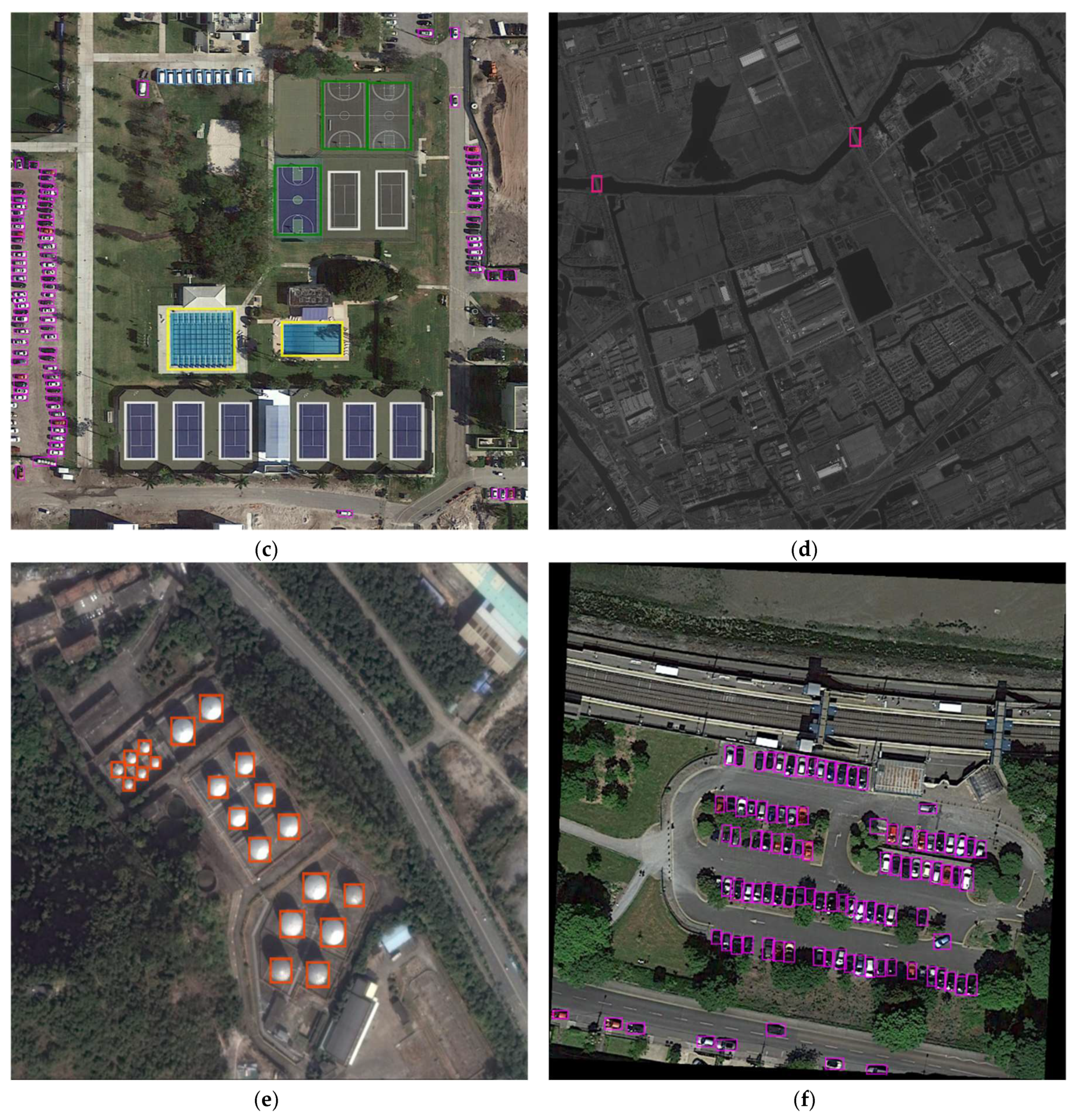
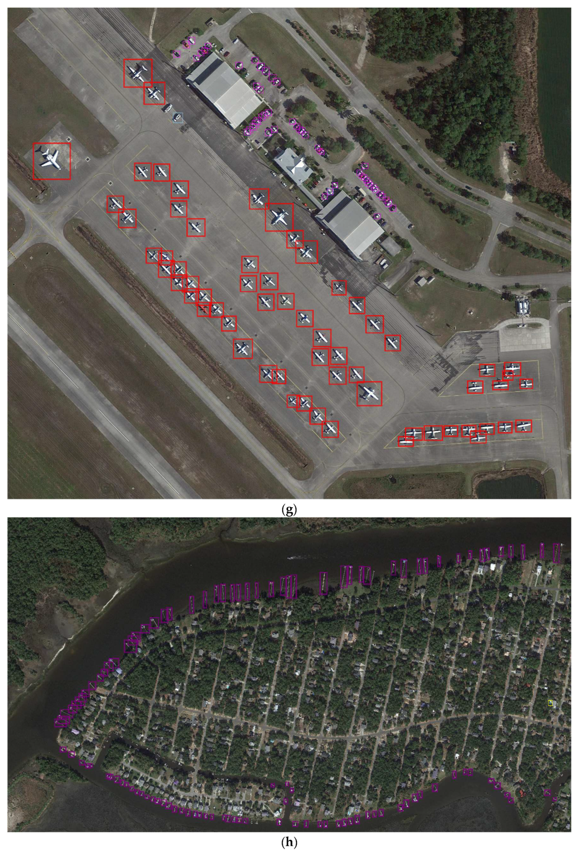
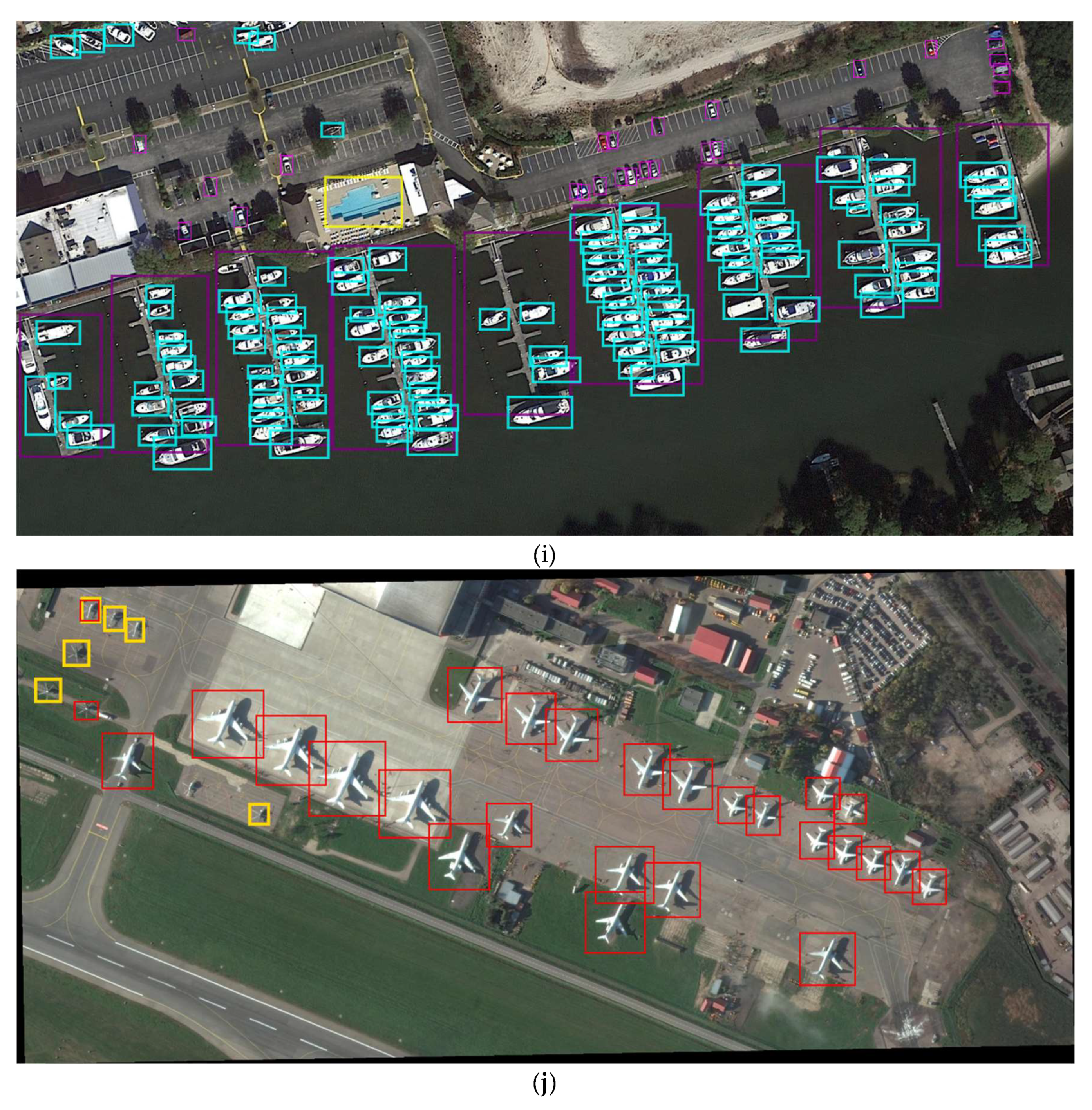
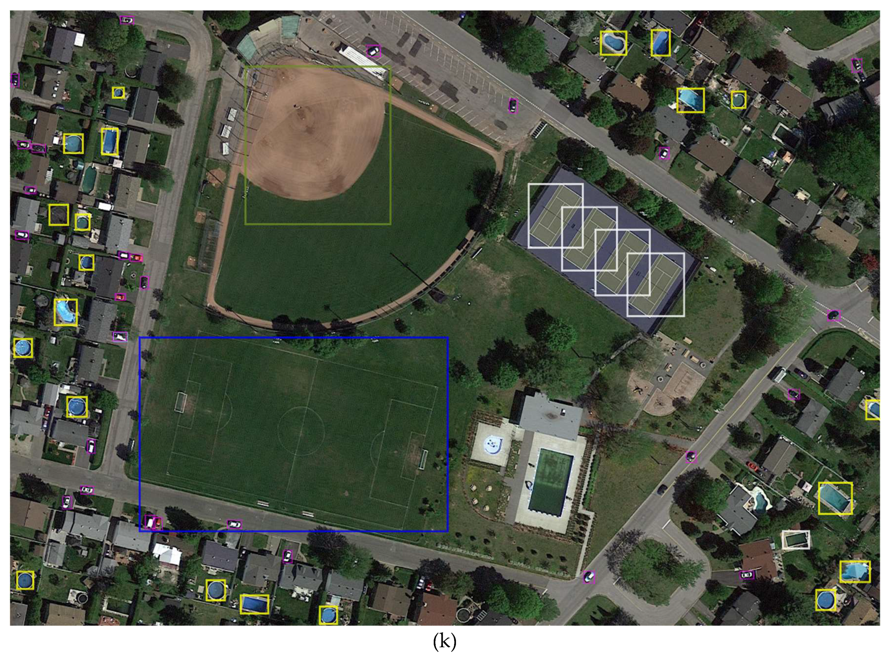
The visualization of the objects detected by SCFPN in the DOTA dataset is shown in Figure 6. The detection results for the object classes of plane, baseball diamond, bridge, ground track field, small vehicle, large vehicle, ship, tennis court white, basketball court, storage tank, soccer field, roundabout, harbor, swimming pool, and helicopter are denoted by pink, beige, deep pink, ivory, purple–red, sky blue, cyan, white, green, orange–red, blue, deep blue, purple yellow, and gold boxes, respectively. Figure 6 shows that the proposed SCFPN not only demonstrates a relatively good detection performance with respect to small and dense targets, such as airplanes, vehicles, ships, and storage tanks, but it also achieves great detection results with respect to large scene objects, such as various kinds of sports courts, harbors, roundabouts, and bridges.
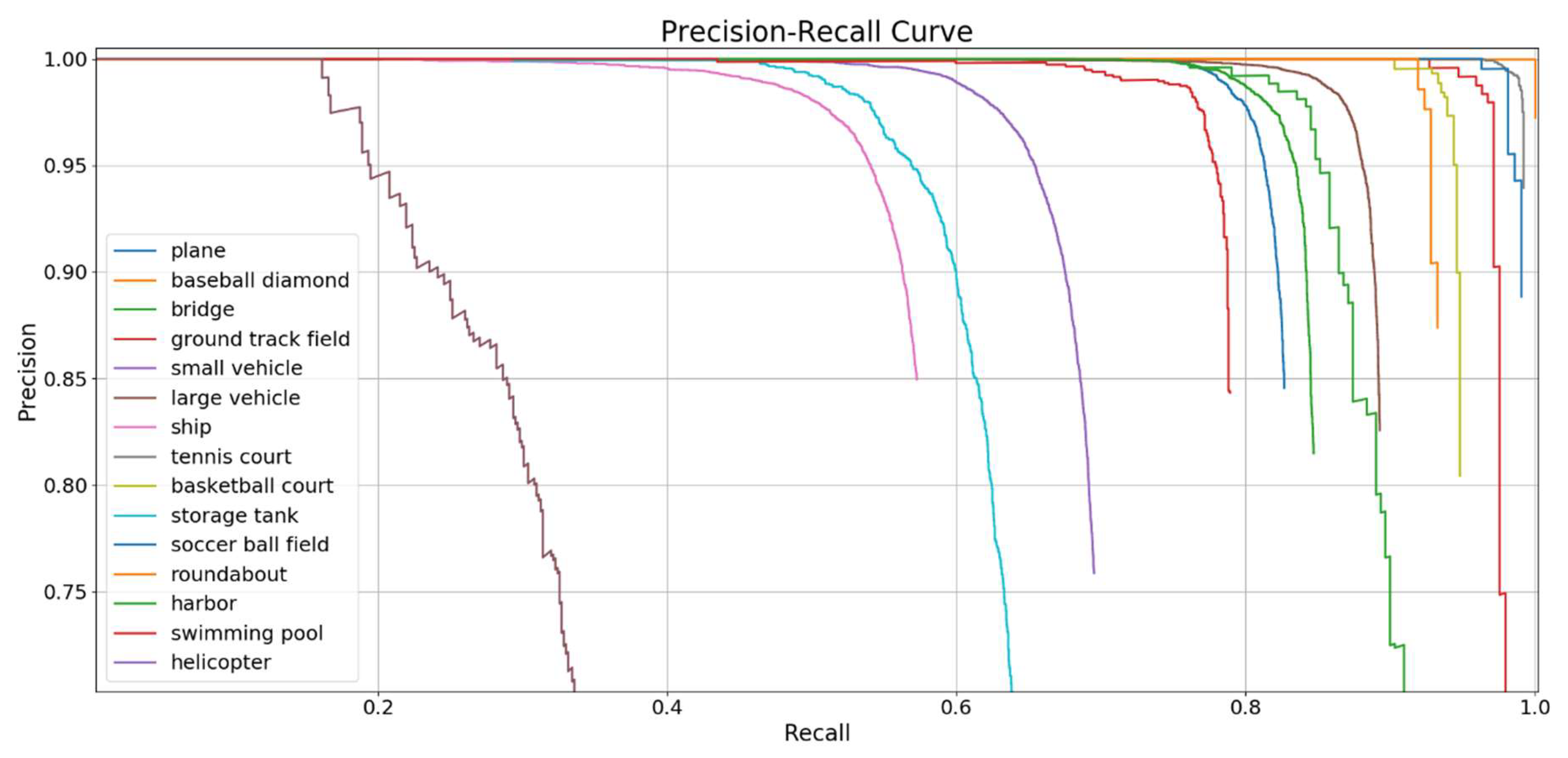
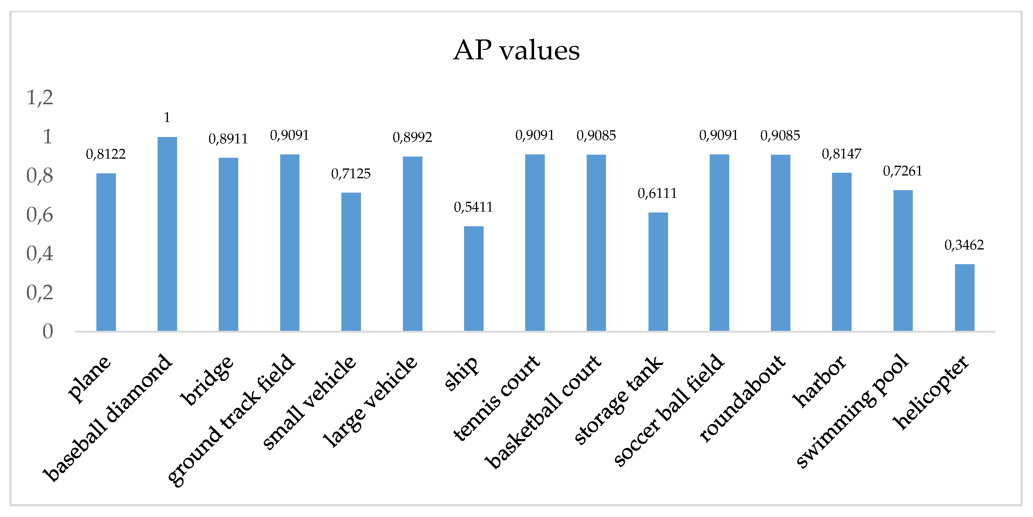
Figure 7 shows the precision-recall curves over the 15 testing classes. The recall ratio evaluates the ability to detect more targets, while the precision evaluates the quality of the detection of correct objects rather than false alarms. Thus, the bigger the recall value with a sharp decline of the curve, the better the recognition performance of the class. As can be seen in Figure 7, the precision-recall curves of 10 object classes show a sharp decline when the recall value exceeds 0.8. The AP values of different classes of targets are shown in Figure 8. Figure 8 shows that the proposed method achieves great performance on the 15-class detection task. Specifically, there are six target classes exceeding a 0.9 AP value, which are the baseball diamond, ground track field, tennis court, basketball court, soccer field, and roundabout classes. For the small and dense targets, such as large vehicles and planes, we also achieved great detection results for which the AP values are 0.8992 and 0.8122, respectively. However, our model is not ideal for detecting helicopters. There are two main causes of this result. First, the number of samples of helicopters for training and testing are fewer than those of the other target classes, which leads to unbalanced training and low detection accuracy. Second, the helicopter samples nearly always appear at the same time as the plane samples, and helicopters and planes are often located in airport scenes, which will lead to the erroneous detection of helicopters as planes.
4.2. Comparative Experiment
In the comparative experiment, we performed a series of experiments on the DOTA dataset, and the proposed method achieved a state-of-the-art level performance of 79.32% for the mAP. Table 3 shows the comparison of the mAP results of the various detection methods.
In Table 3, it can be seen that the R-FCN [4] and faster R-CNN have poor performance because of the lack of an FPN framework. Faster FPN, which uses the FPN framework based on faster R-CNN, achieves a great improvement over the faster R-CNN model. To evaluate the effect of the proposed SCFPN, we designed the contrast experiments, considering the use of the scene-contextual feature, group normalization layer, and ResNeXt-d, respectively.
The advantages of fusing the scene-contextual feature are that it can enhance the correlation between the target and scene, reduce errors in the ROI classification, and improve the detection performance. To verify the helpfulness of fusing scene-contextual feature, we designed two sets of comparative experiments: (faster FPN-1, SCFPN-1) and (faster FPN-2, SCFPN-2). The main difference between the two groups of experiments is the backbone network, because both faster FPN-1 and SCFPN-1 use ResNeXt-101 as the backbone network and both faster FPN-2 and SCFPN-2 use ResNeXt-d-101. It can be seen that the SCFPN-1 fusing scene-contextual feature leads to a 2.54% performance improvement over faster FPN-1. In addition, the SCFPN-2 fusing scene-contextual feature also achieves better performance than faster FPN-2.
The comparison of faster FPN, faster FPN-1, and faster FPN-2 was designed to verify the effectiveness of the proposed ResNeXt-d blocks. Faster FPN-1, which uses the ResNeXt backbone network, achieves a 1.62% performance improvement over faster FPN, which uses the ResNet backbone network. Faster FPN-2 uses ResNeXt-d as the backbone network, and this leads to a further 1.37% improvement over faster FPN-1.
The GN layer was used to solve the limitations of the BN layer. In the experiments, both SCFPN-3 and faster FPN-3 used the GN layer to replace the BN layer. Compared with SCFPN-2 and faster FPN-2, which still use the BN layer, the GN layer methods achieved better performance.
In all of the comparison experiments, SCFPN-3, which has the fusing scene-contextual feature, uses ResNeXt-d as the backbone network, and uses a GN layer, shows the best improvement and achieves the highest mAP value of 79.32%.
Table 4 shows the value of F1 for each method. It can be seen that the proposed method also achieves the highest F1 value of 72.44%.
Table 5 presents the average testing time per image for each method. It is seen that the method we proposed ensures performance improvement while keeping the testing time at a relatively fast level.
To further evaluate the stability of the proposed method, cross-validation was adopted in the comparative experiment. We divided the DOTA dataset into five parts: four of them were used as training data, and one was used as testing data. We obtained the five results by executing five experiments respectively and calculating the average value of the five results as the final results. Table 5 shows the final cross-validation results for each method. As shown in Table 6, the proposed method has stable performance and achieves the highest mAP value of 78.69% and the highest F1 value of 73.11%.
4.3. Discussion
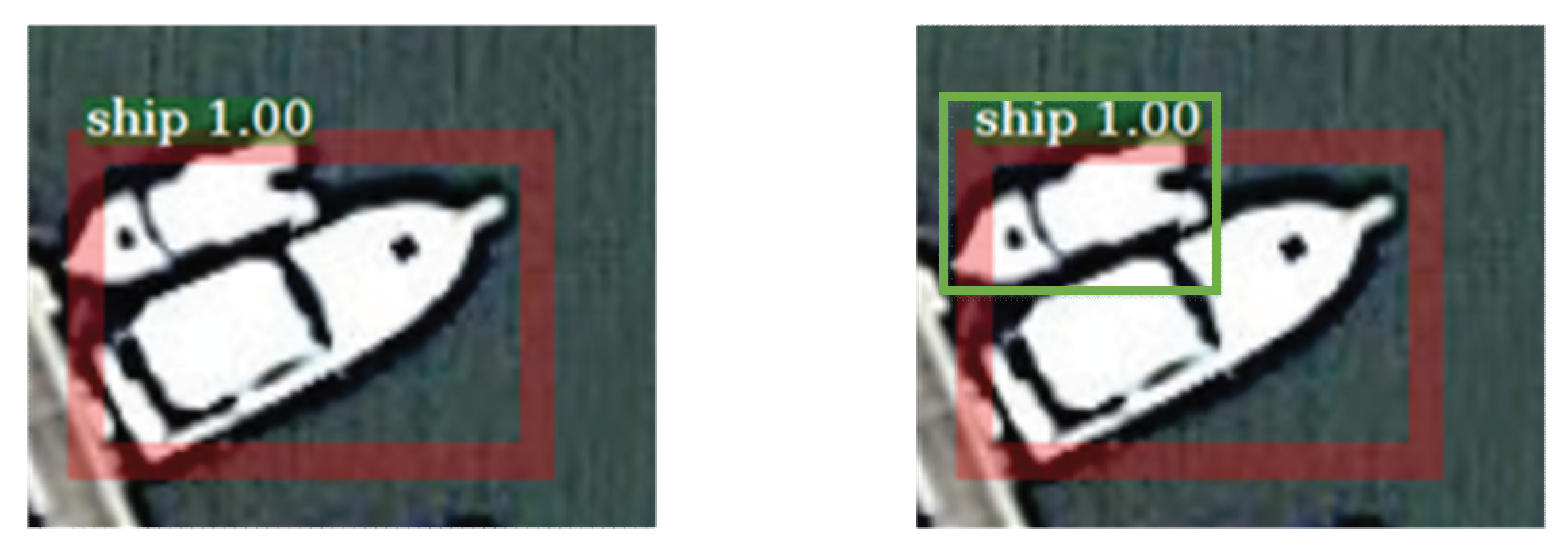
By comparing and analyzing the groups of experiments, the validity of the proposed method was verified. SCFPN offers superior performance with respect to both multi-scale and high-density objects. However, it can be seen from Figure 8 that the ship detection demonstrates poor performance. We visualized the detection results for the class of ships and found that many ships were undetected in the results. Figure 9 shows a common undetected case, contrasting a detected result by the proposed SCFPN (left) and the ground-truth target (right; the green box denotes the undetected ship). Figure 9 shows that the value of IOU between the detected ship and the undetected ship is over 0.7. However, in our method, we used non-maximum suppression (NMS) to process the overlap boxes, which regards an IOU value between boxes of over 0.7 as the same target and only keeps one detected box with the maximum prediction value. Therefore, for dense, small, and oriented objects (such as ships and vehicles), the use of horizontal bounding boxes for detection makes it easy to eliminate a ground-truth target that has high value of IOU between other targets. We also tried to use soft-NMS to solve this problem, but the effect of the improvement was not significant.
Thus, the use of horizontal bounding boxes for detection is the greatest limitation of our model. Perhaps using oriented bounding boxes could provide better solution to this problem and further improve the performance. This is an issue that should be addressed in future studies.
5. Conclusions
In this paper, we proposed an efficient method for multi-sized object detection in remote sensing images. The proposed method has the following novel features: 1) a scene-contextual feature pyramid network (SCFPN), which is based on a multi-scale detection framework, is proposed to enhance the relationship between the target and the scene and ensure the effectiveness of the detection of multi-scale objects; 2) a combination block structure called ResNeXt-d is applied in the backbone network to increase the receptive field and extract richer information for small targets; and 3) we use the GN layer to solve the limitation of the BN layer and eventually achieve a better performance. The experimental results on the public and challenging DOTA dataset and the comparisons with state-of-the-art methods demonstrate the effectiveness and superiority of the proposed method. With the use of the multi-scale framework, our proposal is shown to be effective in detecting multi-scale objects. However, despite demonstrating the best performance, our method utilizes horizontal bounding boxes to detect targets, and this can lead to the failure to detect dense targets. Thus, our future work will focus on investigating a detection framework with oriented bounding boxes to improve the performance of our proposed model.
Author Contributions
The work presented in this paper was developed collaboratively by all the authors. W.G. is the corresponding author of this research work. C.C. proposed the whole detection framework and designed and conducted the experiments. Y.C. was involved in experimental analysis. W.L. was involved in the writing and argumentation of the manuscript. All the authors discussed and approved the final manuscript.
Funding
This work was funded by the Key Projects of Science and Technology Agency of Guangxi province, China (Guike AA 17129002); National Science and Technology Key Program of China (2013GS500303); and the Municipal Science and Technology Project of CQMMC, China (2017030502).
Acknowledgments
We acknowledge the use of DOTA dataset which acquired from the DOTA website (http://captain.whu.edu.cn/dotaweb/index.html). We are also very grateful for the valuable suggestions and comments of peer reviewers.
Conflicts of Interest
The authors declare no conflicts of interest.
References
- Krizhevsky, A.; Sutskever, I.; Hinton, G.E. ImageNet classification with deep convolutional neural networks. In Proceedings of the International Conference on Neural Information Processing Systems (NIPS), Lake Tahoe, NV, USA, 3–6 December 2012; pp. 1097–1105. [Google Scholar]
- Simonyan, K.; Zisserman, A. Very Deep Convolutional Networks for Large-Scale Image Recognition. arXiv, 2014; arXiv:1409.1556. [Google Scholar]
- Szegedy, C.; Liu, W.; Jia, Y.; Jia, Y.Q.; Sermanet, P. Going deeper with convolutions. In Proceedings of the IEEE International Conference on Computer Vision and Pattern Recognition (CVPR), Boston, MA, USA, 7–12 June 2015; pp. 1–9. [Google Scholar]
- Dai, J.F.; Li, Y.; He, K.M.; Sun, J. R-FCN: Object Detection via Region-based Fully Convolutional Networks. arXiv, 2016; arXiv:1606.06409. [Google Scholar]
- Girshick, R.; Donahue, J.; Darrell, T.; Malik, J. Rich feature hierarchies for accurate object detection and semantic segmentation. In Proceedings of the IEEE Conference on Computer Vision and Pattern Recognition (CVPR), Columbus, OH, USA, 23–28 June 2014; pp. 580–587. [Google Scholar]
- Wang, Q.; Wan, J.; Yuan, Y. Locality Constraint Distance Metric Learning for Traffic Congestion Detection. Pattern Recognition. 2018, 75, 272–281. [Google Scholar] [CrossRef]
- Wang, Q.; Chen, M.; Nie, F.; Li, X. Detecting Coherent Groups in Crowd Scenes by Multiview Clustering. TPAMI 2018. [Google Scholar] [CrossRef]
- Yuan, Y.; Xiong, Z.; Wang, Q. An Incremental framework for Video-based Traffic Sign Detection, Tracking and Recognition. ITSM 2016, 18, 1918–1929. [Google Scholar] [CrossRef]
- Girshick, R.; Donahue, J.; Darrell, T.; Malik, J. Region-Based Convolutional Networks for Accurate Object Detection and Segmentation. TRAMPI 2015, 38, 142–158. [Google Scholar] [CrossRef]
- Uijlings, J.R.R.; Sande, K.; Gevers, T.; Smeulders, A.W.M. Selective Search for Object Recognition. Int. J. Comput. Vis. 2013, 104, 154–171. [Google Scholar] [CrossRef]
- Girshick, R. Fast R-CNN. In Proceedings of the IEEE International Conference on Computer Vision, Santiago, Chile, 11–18 December 2015; pp. 1440–1448. [Google Scholar]
- Ren, S.; He, K.; Girshick, R.; Sun, J. Faster R-CNN: Towards Real-Time Object Detection with Region Proposal Networks. TRAMPI 2017, 39, 1137–1149. [Google Scholar] [CrossRef]
- Zeng, D.; Zhao, F.; Ge, S.; Shen, W. Fast cascade face detection with pyramid network. Pattern Recognit. Lett. 2018. [Google Scholar] [CrossRef]
- Liu, W.; Anguelov, D.; Erhan, D.; Szegedy, C.; Fu, C.; Berg, A.C. SSD: Single Shot Multibox Detector. In Proceedings of the European Conference on Computer Vision, Amsterdam, The Netherlands, 8–16 October 2016; pp. 21–37. [Google Scholar]
- Lin, T.Y.; Dollár, P.; Girshick, R.; He, K.; Hariharan, B.; Belongie, S. Feature pyramid networks for object detection. arXiv, 2017; arXiv:1612.03144. [Google Scholar]
- Vakalopoulou, M.; Karantzalos, K.; Komodakis, N.; Paragios, N. Building detection in very high resolution multispectral data with deep learning features. In Proceedings of the IEEE International Geoscience and Remote Sensing Symposium (IGARSS), Milan, Italy, 26–31 July 2015; pp. 1873–1876. [Google Scholar]
- Ammour, N.; Alhichri, H.; Bazi, Y.; Benjdira, B.; Alajlan, N.; Zuair, M. Deep Learning Approach for Car Detection in UAV Imagery. Remote Sens. 2017, 9, 312. [Google Scholar] [CrossRef]
- Zhang, L.; Shi, Z.; Wu, J. A Hierarchical Oil Tank Detector with Deep Surrounding Features for High-Resolution Optical Satellite Imagery. IEEE J. STARS 2017, 8, 1–15. [Google Scholar] [CrossRef]
- Long, Y.; Gong, Y.; Xiao, Z.; Liu, Q. Accurate Object Localization in Remote Sensing Images Based on Convolutional Neural Networks. IEEE Geosci. Remote Sens. 2017, 55, 2486–2498. [Google Scholar] [CrossRef]
- Zhang, F.; Du, B.; Zhang, L.P.; Xu, M.Z. Weakly Supervised Learning Based on Coupled Convolutional Neural Networks for Aircraft Detection. IEEE Geosci. Remote Sens. 2016, 54, 5553–5563. [Google Scholar] [CrossRef]
- Maggiori, E.; Tarabalka, Y.; Charpiat, G.; Alliez, P. Convolutional Neural Networks for Large-Scale Remote-Sensing Image Classification. IEEE Geosci. Remote Sens. 2016, 55, 645–657. [Google Scholar] [CrossRef]
- Sun, L.; Tang, Y.; Zhang, L. Rural Building Detection in High-Resolution Imagery Based on a Two-Stage CNN Model. IEEE Geosci. Remote Sens. Lett. 2017, 14, 1998–2002. [Google Scholar] [CrossRef]
- Cheng, G.; Zhou, P.; Han, J. Learning Rotation-Invariant Convolutional Neural Networks for Object Detection in VHR Optical Remote Sensing Images. IEEE Geosci. Remote Sens. 2016, 54, 7405–7415. [Google Scholar] [CrossRef]
- Chen, C.Y.; Gong, W.G.; Hu, Y.; Chen, Y.L.; Ding, Y. Learning Oriented Region-based Convolutional Neural Networks for Building Detection in Satellite Remote Sensing Images. Int. Arch. Photogramm. Remote Sens. Spat. Inf. Sci. 2017, XLII-1/W1, 461–464. [Google Scholar] [CrossRef]
- Deng, Z.; Sun, H.; Zhou, S.; Zhao, J.; Lei, L.; Zou, H. Multi-scale object detection in remote sensing imagery with convolutional neural networks. ISPRS J. Photogramm. Remote Sens. 2018, 145, 3–22. [Google Scholar] [CrossRef]
- Guo, W.; Yang, W.; Zhang, H.; Hua, G. Geospatial Object Detection in High Resolution Satellite Images Based on Multi-Scale Convolutional Neural Network. Remote Sens. 2018, 10, 131. [Google Scholar] [CrossRef]
- Yang, X.; Sun, H.; Fu, K.; Yang, J.; Sun, X.; Yan, M.; Guo, Z. Automatic Ship Detection in Remote Sensing Images from Google Earth of Complex Scenes Based on Multiscale Rotation Dense Feature Pyramid Networks. Remote Sens. 2018, 10, 132. [Google Scholar] [CrossRef]
- Yu, B.; Yang, L.; Chen, F. Semantic Segmentation for high spatial resolution remote sensing images based on convolution neural network and pyramid pooling module. IEEE J. STARS 2018, 99, 1–10. [Google Scholar] [CrossRef]
- Xia, G.S.; Bai, X.; Ding, J.; Zhu, Z.; Belongie, S.; Luo, J.; Datcu, M.; Pelillo, M.; Zhang, L. DOTA: A Large-scale Dataset for Object Detection in Aerial Images. arXiv, 2017; arXiv:1711.10398. [Google Scholar]
- He, K.; Gkioxari, G.; Dollar, P.; Girshick, R. Mask R-CNN. IEEE Trans. Pattern Anal. Mach. Intell. 2017, 99, 1-1. [Google Scholar] [CrossRef]
- Xie, S.; Girshick, R.; Dollar, P.; Tu, Z.; He, K. Aggregated Residual Transformations for Deep Neural Networks. arXiv, 2017; arXiv:1611.05431. [Google Scholar]
- Yu, F.; Koltun, V. Multi-Scale Context Aggregation by Dilated Convolutions. arXiv, 2015; arXiv:1511.07122. [Google Scholar]
- He, K.; Zhang, X.; Ren, S.; Sun, J. Deep Residual Learning for Image Recognition. In Proceedings of the IEEE Conference on Computer Vision and Pattern Recognition (CVPR), Las Vegas, NV, USA, 26–30 June 2016; pp. 770–778. [Google Scholar]
- Ioffe, S.; Szegedy, C. Batch normalization: accelerating deep network training by reducing internal covariate shift. In Proceedings of the International Conference on International Conference on Machine Learning, Lille, France, 6–11 July 2015; pp. 448–456. [Google Scholar]
- Wu, Y.X.; He, K.M. Group Normalization. arXiv, 2018; arXiv:1803.08494. [Google Scholar]
- Gao, X.; Sun, X.; Zhang, Y.; Yan, M.; Xu, G.; Sun, X.; Jiao, J.; Fu, K. An end-to-end neural network for road extraction from remote sensing imagery by multiple feature pyramid network. IEEE Access. 2018, 6, 39401–39414. [Google Scholar] [CrossRef]
- Girshick, R.; Radosavovic, I.; Gkioxari, G.; Dollar, P.; He, K. Detectron. Available online: https://github.com/facebookresearch/detectron (accessed on 22 January 2018).
Figure 1.
Framework of the proposed scene-contextual feature pyramid network (SCFPN). ROI: region of interest; FPN: feature pyramid network; Fc: fully convolutional layer; cls: classification.
Figure 1.
Framework of the proposed scene-contextual feature pyramid network (SCFPN). ROI: region of interest; FPN: feature pyramid network; Fc: fully convolutional layer; cls: classification.

Figure 2.
Architecture of the proposed region proposal network based on a feature pyramid network (FPN-RPN).
Figure 2.
Architecture of the proposed region proposal network based on a feature pyramid network (FPN-RPN).

Figure 3.
Architecture of different blocks. (a) ResNet; (b) ResNeXt; and (c) ResNeXt-d.

Figure 4.
Normalization methods. Each subplot shows a feature map tensor, with N as the batch axis, C as the channel axis, and (H, W) as the spatial axes. The pixels in blue are normalized by the same mean and variance, computed by aggregating the values of these pixels.
Figure 4.
Normalization methods. Each subplot shows a feature map tensor, with N as the batch axis, C as the channel axis, and (H, W) as the spatial axes. The pixels in blue are normalized by the same mean and variance, computed by aggregating the values of these pixels.

Figure 5.
Samples of the 15-class geospatial object detection dataset.

Figure 6.
Visualization of the objects detected by SCFPN in the DOTA dataset. (a) swimming pool; (b) swimming pool, small vehicle, and roundabout; (c) small vehicle, large vehicle, basketball court, swimming pool, and tennis court; (d) bridge; (e) storage tank; (f) small vehicle; (g) plane and small-vehicle; (h) harbor; (i) boat, small vehicle, harbor, and swimming pool; (j) plane and helicopter; and (k) baseball diamond, tennis court, small vehicle, swimming pool, and soccer field.


Figure 7.
The precision-recall curves of different classes in the proposed method.

Figure 8.
The average precision (AP) values of the different classes in the proposed method.

Figure 9.
A common case of missed detection. The red box denotes the detected result and the green box (right) denotes the undetected object.
Figure 9.
A common case of missed detection. The red box denotes the detected result and the green box (right) denotes the undetected object.


Table 1.
Analysis results of the training part of the DOTA dataset.
| Object Classes | Number of Images | Number of Relevant Scenes Images |
|---|---|---|
| Ground track field | 177 | 138 (scenes of sports areas) |
| Ship | 326 | 318 (scenes of rivers and seas) |
| Soccer field | 136 | 105 (scenes of sports areas) |
| Helicopter | 30 | 30 (scenes of airplanes) |
| Large vehicle | 380 | 380 (scenes of roads and parking lots) |
| Small vehicle | 486 | 480 (scenes of roads and parking lots) |
| Bridge | 210 | 210 (scenes of rivers) |
| Baseball diamond | 122 | 122 (scenes of sports areas) |
| Tennis court | 302 | 278 (scenes of sports areas) |
| Roundabout | 170 | 169 (scenes of crossroads) |
| Plane | 197 | 193 (scenes of airplanes) |
| Basketball court | 111 | 102 (scenes of sports areas) |
| Swimming pool | 144 | 143 (scenes of sports and residential areas) |
| Storage tank | 161 | 158 (scenes of country) |
| Harbor | 339 | 339 (scenes of rivers and seas) |
Table 2.
Structure of 50 layers of the three backbone networks.
| Stage | Output | ResNet-50 | ResNeXt-50 | ResNeXt-d-50 |
|---|---|---|---|---|
| C1 | 112112 | 77, 64 | 77, 64 | 77, 64 |
| C2 | 56 56 | 33 max pool | 33 max pool | 33 max pool |
| C3 | 2828 | |||
| C4 | 1414 | |||
| C5 | 77 | |||
| 11 | 15-d fc, softmax | 15-d fc, softmax | 15-d fc, softmax | |
| Parameter Scale | ||||
Table 3.
Comparison of the mean average precision (mAP) results. SC: scene-contextual framework; FPN: feature pyramid network; GN: group normalization layer; R-CNN: region-based convolutional neural network. 101 means the model with 101 layers. The bold result is the best performance value.
Table 3.
Comparison of the mean average precision (mAP) results. SC: scene-contextual framework; FPN: feature pyramid network; GN: group normalization layer; R-CNN: region-based convolutional neural network. 101 means the model with 101 layers. The bold result is the best performance value.
| Detection Methods | Backbone | SC | FPN | GN | mAP (%) |
|---|---|---|---|---|---|
| R-FCN [4] | ResNet-101 | - | - | - | 45.63 |
| Faster R-CNN | ResNet-101 | - | - | - | 49.18 |
| Faster FPN | ResNet-101 | - | √ | - | 71.36 |
| Faster FPN-1 | ResNeXt-101 | - | √ | - | 72.68 |
| Faster FPN-2 | ResNeXt-d-101 | - | √ | - | 74.31 |
| Faster FPN-3 | ResNeXt-d-101 | - | √ | √ | 75.65 |
| SCFPN-1 | ResNeXt-101 | √ | √ | - | 75.22 |
| SCFPN-2 | ResNeXt-d-101 | √ | √ | - | 77.63 |
| SCFPN-3 | ResNeXt-d-101 | √ | √ | √ | 79.32 |
Table 4.
Comparison of the F1 results. The bold result is the best performance value.
| Method | R-FCN | Faster RCNN | Faster FPN | SCFPN-1 | SCFPN-2 | SCFPN-3 |
|---|---|---|---|---|---|---|
| F1 (%) | 36.68 | 40.84 | 60.02 | 66.97 | 69.15 | 72.44 |
Table 5.
The average testing time for the different methods.
| Method | R-FCN | Faster RCNN | Faster FPN | SCFPN-1 | SCFPN-2 | SCFPN-3 |
|---|---|---|---|---|---|---|
| Testing Time | 0.18 s | 0.17 s | 0.20 s | 0.22 s | 0.22 s | 0.24 s |
Table 6.
Comparison of the cross-validation results. The bold results are the best performance values.
Table 6.
Comparison of the cross-validation results. The bold results are the best performance values.
| Method | R-FCN | Faster RCNN | Faster FPN | SCFPN-1 | SCFPN-2 | SCFPN-3 |
|---|---|---|---|---|---|---|
| mAP (%) | 41.26 | 46.93 | 70.11 | 74.46 | 76.52 | 78.69 |
| F1 (%) | 37.45 | 41.38 | 59.17 | 66.72 | 69.54 | 73.11 |
© 2019 by the authors. Licensee MDPI, Basel, Switzerland. This article is an open access article distributed under the terms and conditions of the Creative Commons Attribution (CC BY) license (http://creativecommons.org/licenses/by/4.0/).
Share and Cite
MDPI and ACS Style
Chen, C.; Gong, W.; Chen, Y.; Li, W. Object Detection in Remote Sensing Images Based on a Scene-Contextual Feature Pyramid Network. Remote Sens. 2019, 11, 339. https://doi.org/10.3390/rs11030339
AMA Style
Chen C, Gong W, Chen Y, Li W. Object Detection in Remote Sensing Images Based on a Scene-Contextual Feature Pyramid Network. Remote Sensing. 2019; 11(3):339. https://doi.org/10.3390/rs11030339
Chicago/Turabian StyleChen, Chaoyue, Weiguo Gong, Yongliang Chen, and Weihong Li. 2019. "Object Detection in Remote Sensing Images Based on a Scene-Contextual Feature Pyramid Network" Remote Sensing 11, no. 3: 339. https://doi.org/10.3390/rs11030339
Note that from the first issue of 2016, this journal uses article numbers instead of page numbers. See further details here.