Enhanced Regional Monitoring of Wheat Powdery Mildew Based on an Instance-Based Transfer Learning Method

Abstract

In order to monitor the prevalence of wheat powdery mildew, current methods require sufficient sample data to obtain results with higher accuracy and stable validation. However, it is difficult to collect data on wheat powdery mildew in some regions, and this limitation in sampling restricts the accuracy of monitoring regional prevalence of the disease. In this study, an instance-based transfer learning method, i.e., TrAdaBoost, was applied to improve the monitoring accuracy with limited field samples by using auxiliary samples from another region. By taking into account the representativeness of contributions of auxiliary samples to adjust the weight placed on auxiliary samples, an optimized TrAdaBoost algorithm, named OpTrAdaBoost, was generated to map regional wheat powdery mildew. The algorithm conducts this by: (1) producing uncertainty associated with each prediction based on the similarities, and calculating the representativeness contribution of all auxiliary samples by taking into account the overall uncertainty of the wheat powdery mildew map; (2) calculating the errors of the weak learners during the training process and using boosting to filter out the unreliable auxiliary samples by adjusting the weights of auxiliary samples; (3) combining all weak learners according to the weights of training instances to build a strong learner to classify disease severity. OpTrAdaBoost was tested using a dataset with 39 study area samples and 106 auxiliary samples. The overall monitoring accuracy was 82%, and the kappa coefficient was 0.72. Moreover, OpTrAdaBoost performed better than other algorithms that are commonly used to monitor wheat powdery mildew at the regional level. Experimental results demonstrated that OpTrAdaBoost was effective in improving the accuracy of monitoring wheat powdery mildew using limited field samples.

1. Introduction

Wheat powdery mildew is caused by the fungus Blumeria graminis and is one of the most common diseases that result in significant loss of crop yield and quality in China [1,2,3]. Recently, wheat powdery mildew has spread from Southwestern China to Eastern and Northern China. In addition to its wider geographic range, the disease has also become more frequent and severe over the years [1,4]. According to the statistics of the China’s National Agricultural Technology Extension and Service Center (NATESC), the annual average outbreak area for powdery mildew was 10 million ha over the last 17 years [5]. Accurate monitoring of wheat powdery mildew at the regional level is important for food security and environmental protection [6]. Traditionally, wheat powdery mildew is monitored by visual inspection of individual plants, which is time-consuming and inefficient [7]. In recent years, a new satellite-based remote sensing technology has become a more viable option for managing and controlling agricultural practices [3,6,8,9,10].

Wheat powdery mildew is monitored by remote sensing technologies based on changes in transpiration rate, chlorosis, leaf color, and morphology in infected plants, which in turn affects the spectral reflectance properties of wheat [8]. Wheat powdery mildew occurrence and severity at the regional level are currently modeled using statistical analysis and machine learning methods. Statistical analysis methods, such as regression analysis, discriminant analysis, and distance analysis could be used to fit the relationship between the occurrence and severity of wheat powdery mildew and spectral features. In these methods, the spectral features that are sensitive to the wheat powdery mildew are selected and the mathematical model is directly built to provide accurate identification of the disease [11,12,13,14,15]. Machine learning methods, such as decision tree, support vector machine (SVM), and Bayes classification, can learn from samples and devise complex models to detect the relationship between wheat powdery mildew and spectral features. The machine learning algorithms can achieve data-driven modeling, and therefore, models can overcome following strictly static program instructions [16,17,18].

The existing methods for monitoring wheat powdery mildew at the regional level do not always meet the needs of agricultural management due to the difficulty of collecting field samples [19]. In general, data from intensive ground surveys is required to model wheat powdery mildew and to validate the model, but there are several factors that make the collection of wheat powdery mildew data difficult. Wheat powdery mildew symptoms are visible at the end of booting stage (Zadoks stage 4) through to the milk-ripening stage (Zadoks stage 7); therefore, the disease can be detected visually for only a short period of time [3]. In addition to this, field sampling is often expensive, since an expert’s interpretation is required to detect the disease, and once field data is collected, the post-processing of data is often time-consuming. Although the development of drones provides an alternative to traditional methods in obtaining field samples spatially, operating with drones requires lots of effort in the preflight phase, flying, and the post-processing of images, and it is often expensive to use drones when a large area of field needs to be monitored. Taken together, it is difficult to collect sufficient field data for wheat powdery mildew, making it difficult to accurately monitor the disease.

Limited training data is a common problem in remote sensing applications. Many approaches have been used to mitigate small training samples, including data augmentation, unsupervised training, and transfer learning [19]. Data augmentation generates a large number of training data using label-preserving transformations [20], such as affine transformations, rotations, and small patch removal, and data augmentation is often applied when processing remote sensing images. Unsupervised training, where training labels are not required, is widely used to detect objects and change [21,22]. Transfer learning is a methodology to accurately classify the data of target domain by using auxiliary domains [23,24], which has been applied in remote sensing to increase the quality and quantity of samples. For example, Othman et al. [25] used labeled data on landscapes from an auxiliary domain to build a land-use classification system. The model performed well on public datasets from University of California Merced and Banja-Luka LU. Ghazi et al. [26] used transfer learning to fine-tune pretrained models, including GoogLeNet, AlexNet, and VGGNet. The authors then developed a classification system for plant identification that achieved an overall accuracy of 80% on the validation set and an overall inverse rank score of 0.752 on the official test set. TrAdaBoost is an instance-based transfer learning method that is used to address inductive transfer learning problems [27]. Lv et al. [28] integrated TrAdaBoost with Bagging (Bootstrap aggregating) to build a concept extraction model. Three datasets named BETH, PARTNERS, and BETHBIO were employed to show the effectiveness of the concept extraction model. The proposed model outperformed the baseline model by 2.3% and 4.4% when the baseline model was trained by training data that was combined from the source domain and the target domain in two experiments of BETH versus PARTNERS and BETHBIO versus PARTNERS, respectively. Li et al. [29] used feature selection and enhanced TrAdaBoost to classify microscopic images of interregional sandstones and generated an effective and valid method to classify images. However, thus far, the use of transfer learning techniques for crop disease monitoring has received limited attention and there are very few studies that explore whether these approaches can improve the accuracy of crop disease minoring.

In this study, we applied TrAdaBoost to improve the monitoring accuracy of wheat powdery mildew with limited study area samples using auxiliary samples from another region. We defined a quantity named ‘Representativeness’, which indicates the ability of sample data to represent the disease severity–features relationships throughout a study area for reliable model calibration or construction. We hypothesized that limited field samples cannot represent the study area, and auxiliary samples could be used to improve the representativeness of study area samples. Taking this into account, we proposed an optimized TrAdaBoost algorithm (OpTrAdaBoost), which took the representativeness contribution of auxiliary data into consideration to adjust the weights of the auxiliary samples, to monitor wheat powdery mildew. The features that can indicate crop growth status and environmental characteristics were used as input of OpTrAdaBoost. The performance of OpTrAdaBoost was evaluated and compared with other commonly used algorithms, including the Mahalanobis distance, partial least square regression, Fisher’s linear discriminant analysis, logistic regression, and support vector machine. We found that different algorithms exhibited different traits in mapping the intensity of powdery mildew, and OpTrAdaBoost performed the best among these algorithms.

2. Materials and Methods

2.1. Study Area and Data

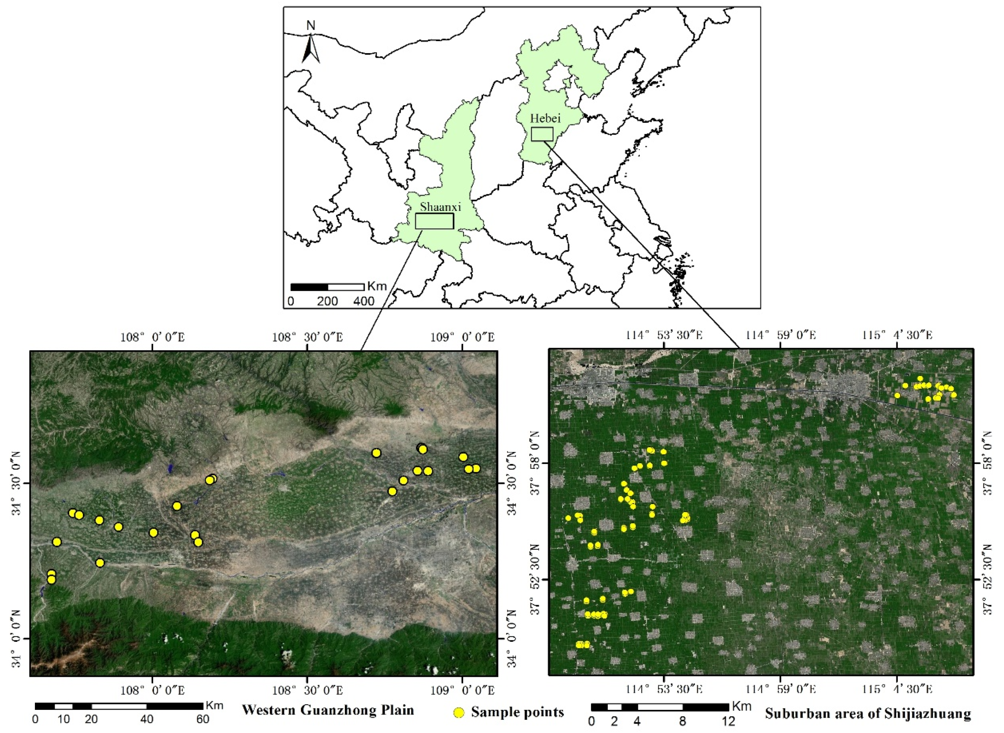
Two field sites were investigated (Figure 1). The study area (108°24′7″E, 34°25′12″N) was the Western Guanzhong Plain, located in Shaanxi province, China, where the major crop type is winter wheat. The region has a temperate humid continental monsoon climate, where the annual mean temperature ranges from 9.9 to 15.8 °C and the annual mean rainfall ranges from 500 to 700 mm [30]. The main land formation of this area is the Weihe Plain, and its terrain is higher in the southern and northern areas and lower in the central and eastern areas [31]. The growing season for wheat is from September to June. Due to the long-term application of organic fertilizers, this region has a fertile agricultural soil, termed Lou soil (manural loessial soil) and classified as Eum-orthic Anthrosol [32]. According to the local agricultural management department, powdery mildew is a common disease in this region.

The auxiliary area (114°57′3″E, 37°55′51″N) was a suburban area of Shijiazhuang, in Hebei province. This region also has a temperate humid continental monsoon climate with an annual mean temperature of 12–13 °C and annual precipitation of 400–800 mm [6,33]. Abundant sunshine and suitable temperature make it suitable for crop growth. The region has concentrated areas of farmland and the growing season for wheat is also from September to June. The major soil type in this region is Haplic Luvisols [34]. Powdery mildew, which is sensitive to local climate and environmental conditions, is reported to be a common disease.

The field survey experiment was arranged in both areas. A total of 145 plots were surveyed for damage caused by wheat powdery mildew as ground truth data in May 2014 (Figure 1). Thirty-nine samples were acquired from the study area, and 106 samples were acquired in the auxiliary area. The sampling design was based on the Rules of Investigation and Forecast of Wheat Powdery Mildew (NY/T 613-2002). Five 1 × 1-m ranges were uniformly selected at a 30 × 30-m spatial range to match the spatial resolution of Landsat 8 images. The central latitude and longitude of each plot were recorded by a submeter precision handheld global positioning system (GPS). The occurrence of wheat powdery mildew was noted in the survey. The disease severity represents the percentage of each leaf that was damaged and it was categorized in 10 classes: 0% (class 0), 1–10% (class 1), 11–20% (class 2), 21–30% (class 3), 31–40% (class 4), 41–50% (class 5), 51–60% (class 6), 61–70% (class 7), 71–80% (class 8), and 81–100% (class 9). After that, the disease index (DI) of each plot was calculated using:

$$DI=\frac{\sum \left(d_i\times l_i\right)}{n\times L}\times 100\%,$$

(1)

where d_i is the class of disease severity, l_i is the number of leaves in each class, n is the highest level of disease severity, and L is the quantity of all selected leaves. Regions were categorized following the guidelines of the National Plant Protection Department [3]: regions with DI = 0% were labeled as normal, regions with 0% < DI ≤ 30% were labeled as slightly diseased, and regions with DI > 30% was labeled as seriously diseased.

The other data used in this study consists of remote sensing data and environmental data, which are summarized in

Table 1. Data used in the study.

Region	Type of Data	Source of Data	Acquired Time	Spatial Resolution	Time Resolution
Western Guanzhong Plain	Remote sensing data	Landsat 8/OLI	2014.5.11	30 m	16 days
	Environmental data	Climate Hazards Group Infrared Precipitation with Station data (CHIRPS) [35]	2014.3.1–2014.5.11	0.05°	1 day
		The MODIS/Terra Land Surface Temperature and Emissivity (LST/E) product (MOD11A1)	2014.3.1–2014.5.11	1 km	1 day
	Field survey data	Fieldwork	2014.5.8—2014.5.10
Suburban area of Shijiazhuang	Remote sensing data	Landsat 8/OLI	2014.5.22	30 m	16 days
	Environmental data	Climate Hazards Group Infrared Precipitation with Station data (CHIRPS)	2014.3.1–2014.5.22	0.05°	1 day
		The MODIS/Terra Land Surface Temperature and Emissivity (LST/E) product (MOD11A1)	2014.3.1–2014.5.22	1 km	1 day
	Field survey data	Fieldwork	2014.5.23—2014.5.28

.

2.2. Remote Sensing Data

A radiometric calibration and an atmospheric correction for Landsat-8 images were conducted using ENVI 5.3 [30]. A radiometric calibration was carried out to convert calibrated digital numbers (DNs) to at-sensor radiance [36]. Atmospheric correction was used to remove the effects of the atmosphere on the reflectance values of images taken by satellite sensors [37]. MOD11A1 generates per-pixel temperature and emissivity values, which are recorded on a daily basis using the generalized split-window LST algorithm [38]. The daily LST of each region was acquired by averaging the daytime LST and nighttime LST.

The temporal dynamics of powdery mildew are primarily influenced by temperature and humidity [39,40], and therefore the average LST and precipitation during March to May was calculated using CHIRPS and daily LST data. The spectral vegetation indices, which are sensitive to wheat powdery mildew, were also utilized to monitor disease. The normalized difference vegetation index (NDVI) and enhanced vegetation index (EVI) were inversed to measure crop growth [41,42,43]. Wetness and greenness, which are generated using tasseled cap transformation, were also inversed to indicate the field habitat characteristics [6]. These indices had been used to monitor wheat powdery mildew in previous studies [6,44] and were calculated using the following equations:

$$NDVI=\frac{{\rho }_{NIR}-{\rho }_{Red}}{{\rho }_{NIR}+{\rho }_{Red}},$$

(2)

$$EVI=G\frac{{\rho }_{NIR}-{\rho }_{Red}}{{\rho }_{NIR}+C_1\times {\rho }_{Red}-C_2\times {\rho }_{Blue}+L},$$

(3)

$$Wetness=w_1\times b_1+w_2\times b_2+w_3\times b_3+w_4\times b_4+w_5\times b_5+w_6\times b_6,$$

(4)

$$Greenness=g_1\times b_1+g_2\times b_2+g_3\times b_3+g_4\times b_4+g_5\times b_5+g_6\times b_6$$

(5)

where ${\rho }_{NIR}$, ${\rho }_{Red}$, and ${\rho }_{Blue}$ in Equations (2) and (3) represent the reflectance of near infrared (NIR), red, and blue, respectively. The values of L, C₁, C₂, and G in Equation (3) were determined using a previous publication [45]. L is the canopy background adjustment that addresses nonlinear, differential NIR, and red radiant transfer through a canopy; G is the gain factor; and C₁ and C₂ are the coefficients of the aerosol resistance term, which uses the blue band to correct for aerosol influences in the red band [46]. The $w_i$ and $g_i$ (i = 1, 2, …, 6) indicate the corresponding coefficient for each band in the Landsat-8 OLI image, and b_i (i = 1, 2, …, 6) indicates the reflectance. The values of $w_i$ and $g_i$ are included in

Table 2. Tasseled cap transformation coefficients for Landsat 8 OLI images.

Index	Band
	1	2	3	4	5	6
	Blue	Green	Red	NIR	SWIR-1	SWIR-2
	0.45–0.51 μm	0.53–0.59 μm	0.64–0.67 μm	0.85–0.88 μm	1.57–1.65 μm	2.11–2.29 μm
Wetness	0.1511	0.1973	0.3283	0.3407	−0.7117	−0.4559
Greenness	−0.2941	−0.243	−0.5424	0.7276	0.0713	−0.1608

.

2.3. Optimized TrAdaBoost Algorithm (OpTrAdaBoost) for Disease Monitoring

TrAdaBoost is a boosting method for transfer learning, which iteratively selects suitable instances from an auxiliary domain to assist in training the accuracy classifier for the target domain by adjusting the weights of labeled instances in both the auxiliary and target domain iteratively [29]. In TrAdaBoost, the training data in the target domain is called same-distribution training data, and the training data in the auxiliary domain is called the diff-distribution training data. In each iteration, all training data is used to train a weak learner and the labels of all training instances are predicted using this weak learner, and then the weights of training instances are adjusted according to the error of the weak learner on these instances. After several iterations, the instances that help the learning algorithm to train better classifiers are selected [47].

The support vector machine with radial basis function kernel (RBFSVM) [48,49] was applied as the weak learner in TrAdaBoost. At the initialization of the algorithm, an initial weight vector w was given, and the initial weight values of all samples were equal. The maximum number of iterations N was also determined. Per iteration, some samples were taken out from the auxiliary samples and study area samples, respectively. The removed samples were used to train a RBFSVM, and the weight of a sample indicated the probability of this sample to be selected to train the RBFSVM. At the end of each iteration, the error of RBFSVM on each training sample was calculated using:

$$erro{r}_i^t=\left|h_t\left(x_i\right)-c\left(x_i\right)\right|,$$

(6)

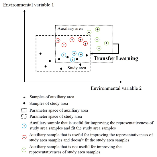
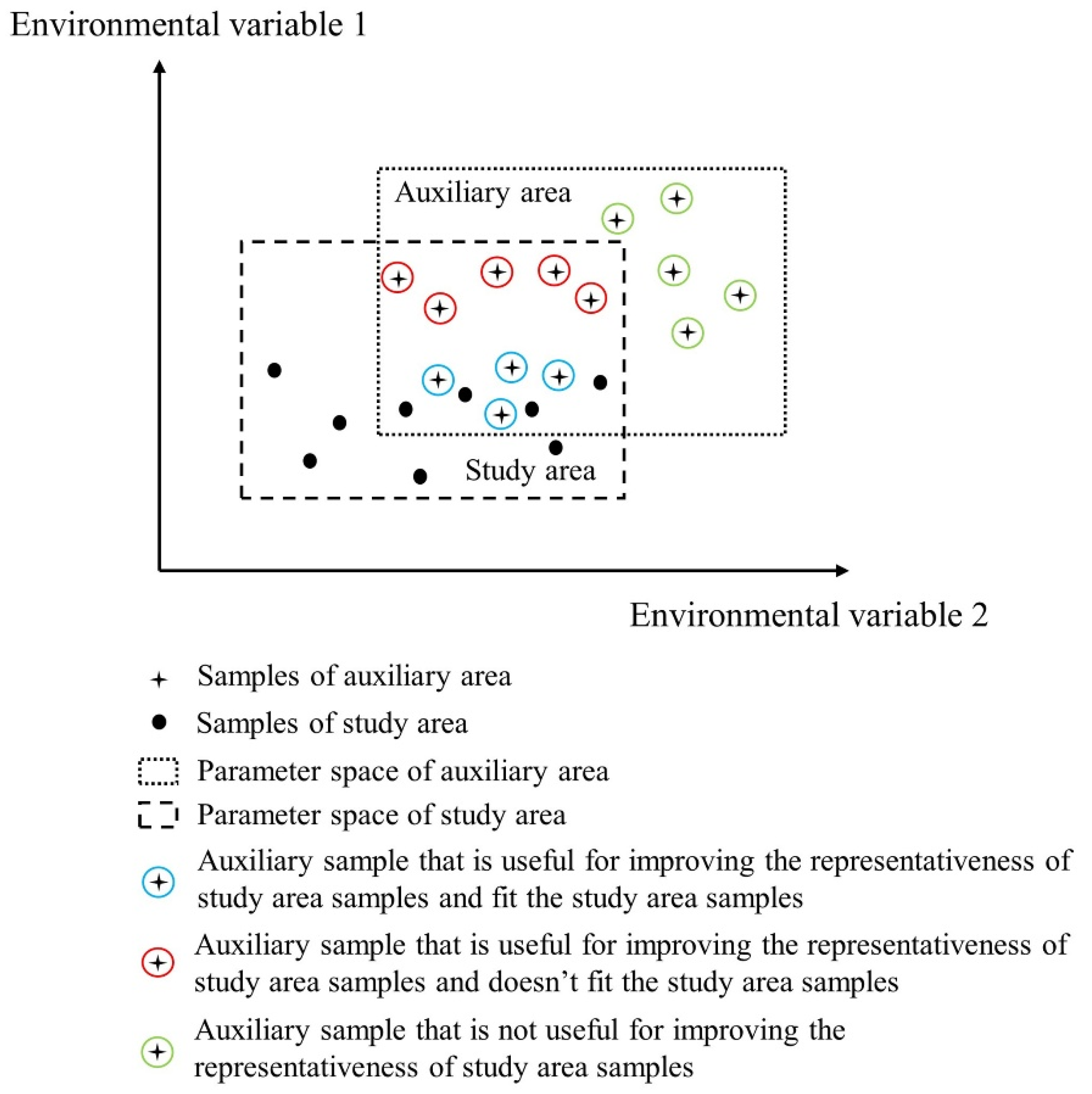
in which $h_t\left(x_i\right)$ is the label of sample i predicted by RBFSVM in the tth iteration and $c\left(x_i\right)$ is the real label of sample i. If an auxiliary training sample was wrongly predicted, the sample likely conflicted with the study area sample. Then, we decreased its weight to reduce its effect, where in the next round, the misclassified auxiliary training sample would affect the learning process less than the previous round. In contrast, if a study area training sample is wrongly predicted, we increased its weight to improve its effect in the next round. Through this mechanism, the auxiliary samples that were useful for improving the representativeness of study area samples and similar to the study area samples were selected (Figure 2, black cross and blue circles).

However, the learning effect of TrAdaBoost was not satisfied if the mechanism for auxiliary weights adjustment relied only on the error of RBFSVM on auxiliary data. This is because RBFSVM discarded auxiliary samples that enriched the representativeness of study area samples but did not fit the study area samples (Figure 2, black cross and red circles). In order to enhance the accuracy of monitoring wheat powdery mildew, we took the representativeness contribution of auxiliary data into consideration when adjusting the auxiliary weights, and created OpTrAdaBoost. The calculation of representativeness contribution is described as follows:

The severity of wheat powdery mildew at the unvisited location of study area was predicted based on similarities to visited locations and disease severity at the visited locations. We produced uncertainty associated with each predication based on the similarities of the locations. In the experiment, the uncertainties of the unvisited locations in the study area were calculated based on samples from the study area. Then, each sample from the auxiliary dataset was added to the study area dataset to reduce the overall uncertainty, and the amount of reduction was used as the representativeness contribution of the auxiliary sample. Specifically, the following steps were taken:

• Calculate similarity at the feature level. Similarity was calculated using NDVI, EVI, wetness, greenness, average LST, and average precipitation. Equation (3) in [50] was used to estimate similarities of unvisited locations to the study area samples at the feature level, because a Gaussian-shaped function is superior in determining their similarities:

  $$S_{v,j,i}=exp\left(\frac{{\left(e_{vj}-e_{vi}\right)}^2}{2{\left(S{D}_{e_v}\times \frac{S{D}_{e_v}}{S{D}_{e_{vi}}}\right)}^2}\right),$$

  (7)

  in which $e_{vj}$ and $e_{vi}$ are values of the vth feature at the two locations, $S{D}_{e_v}$ is the standard deviation of the vth feature in the study area, and $S{D}_{e_{vi}}$ is the square root of the mean deviation of the values of the vth feature at all unvisited locations (j = 1, 2, 3, …, $p$) from that at sample location i; $S{D}_{e_{vi}}$ is quantified as:

  $$S{D}_{e_{vi}}=\sqrt{\frac{{{\displaystyle \sum }}_{j=1}^p{\left(e_{vj}-e_{vi}\right)}^2}{p}}$$

  (8)
• Integrate feature-level similarities at the sample level and evaluate prediction uncertainty at each unvisited location. The weighted average method was used to integrate feature level similarities [51] because features have different weights in the process of disease monitoring. The relative weight for every feature was calculated using a factor analysis [52]. The similarities between an unvisited location j and a study area sample i at the sample level were determined as follows:

  $$S_{j,i}=w_1\times S_{1,j,i}+w_2\times S_{2,j,i}+\dots +w_k\times S_{k,j,i},$$

  (9)

  where $S_{j,i}$ represents the similarity between unvisited location j and sample location i at the sample level,$w_k$ ($k$ is the number of features) is the weight of feature $k$ calculated using factor analysis, and $S_{k,j,i}$ is the similarity between unvisited location j and sample location i at feature $k$, which is calculated in step (i). The prediction uncertainty at each unvisited location was calculated using Equation (6) in [50] because the uncertainty measurement is basically a measurement of how reliable it is to use existing samples to represent a given unvisited location:

  $$Uncertaint{y}_j=1-max\left(S_{j,1}, S_{j,2},\dots , S_{j,m}\right)$$

  (10)

  where $m$ is the size of study area samples, and a larger prediction uncertainty was assigned to unvisited locations that had divergent crop growth status and environmental conditions compared to the study area samples.
• Calculate prediction uncertainty with additional auxiliary samples. An auxiliary sample was added to the study area samples and the prediction uncertainty at each unvisited location was calculated by repeating steps (i) and (ii). After this step, another auxiliary sample was added to the study area samples and the prediction uncertainty at each unvisited location was calculated again. Note that when a new auxiliary sample was added into the study area samples, the previous auxiliary sample was removed, and there was only one auxiliary sample per iteration.
• Evaluate the representativeness contribution of auxiliary samples. Taking auxiliary sample i as an example, the uncertainty maps before and after adding auxiliary sample i were produced through steps (i), (ii), and (iii). The representativeness contribution of auxiliary sample i was quantified as:

  $$Contribution=M_i\times V_i$$

  (11)

  where $M_i$ is the number of pixels at which the prediction uncertainty was reduced after adding auxiliary sample i and $V_i$ is the amount of reduction of overall prediction uncertainty after adding auxiliary sample i.

These four steps were iterated until the representativeness contributions of all auxiliary samples were calculated. Following these steps, a normalization operator was applied to scale the values of representativeness contributions of all auxiliary samples to make them fit in a range from 0 to 1. Eventually, the weight vector was adjusted using the following equations in each iteration:

$$w_i^{t+1}=\{\begin{array}{cc}{w}_i^t{\mathsf{\beta }}^{erro{r}_i^t\times (1-Contributio{n}_i)},\hfill & \hfill 1\le i\le n\\ w_i^t{{\mathsf{\beta }}_t}^{-erro{r}_i^t},\hfill & \hfill n+1\le i\le n+m\end{array},$$

(12)

where $n$ is the size of auxiliary data, $m$ is the size of study area data, and $w_i^t$ is the weight of sample i in the tth iteration. $\mathsf{\beta }$ and ${\mathsf{\beta }}_t$ were defined using a previous publication [47]. $\mathsf{\beta }$ is a change rate for the multiplicative updates of auxiliary weights, which is calculated using $n$ and N, and $\mathsf{\beta }\in \left(0,1\right)$. Note that ${\mathsf{\beta }}^{erro{r}_i^t\times (1-Contributio{n}_i)}$ decreases with the increase of $erro{r}_i^t$ and ${\mathsf{\beta }}^{erro{r}_i^t\times (1-Contributio{n}_i)}$ increases with the increase of $Contributio{n}_i$. Thus, in the next round, the auxiliary samples, which are misclassified in the current round but are useful for improving the representativeness of study area samples, also could have higher weights. ${\mathsf{\beta }}_t$ is a change rate for the multiplicative updates of study area sample weights and ${\mathsf{\beta }}_t\in \left(0,1\right]$, ${\mathsf{\beta }}_t$, and ${{\mathsf{\beta }}_t}^{-erro{r}_i^t}$ all increase with the increase of $erro{r}_i^t$. Thus, the study area samples, which are misclassified in the current round, will have higher weights in the next round. In the end, the labels of unvisited locations were predicted as in the following:

$$h\left(x\right)=\{\begin{array}{cc}1,\hfill & {{\displaystyle \prod }}_{t=⎡\frac{N}{2}⎤}^N{\mathsf{\beta }}_t^{-h_t\left(x\right)}\ge {{\displaystyle \prod }}_{t=\frac{N}{2}}^N{\mathsf{\beta }}_t^{-\frac{1}{2}}\hfill \\ 0,\hfill & otherwise\hfill \end{array}$$

(13)

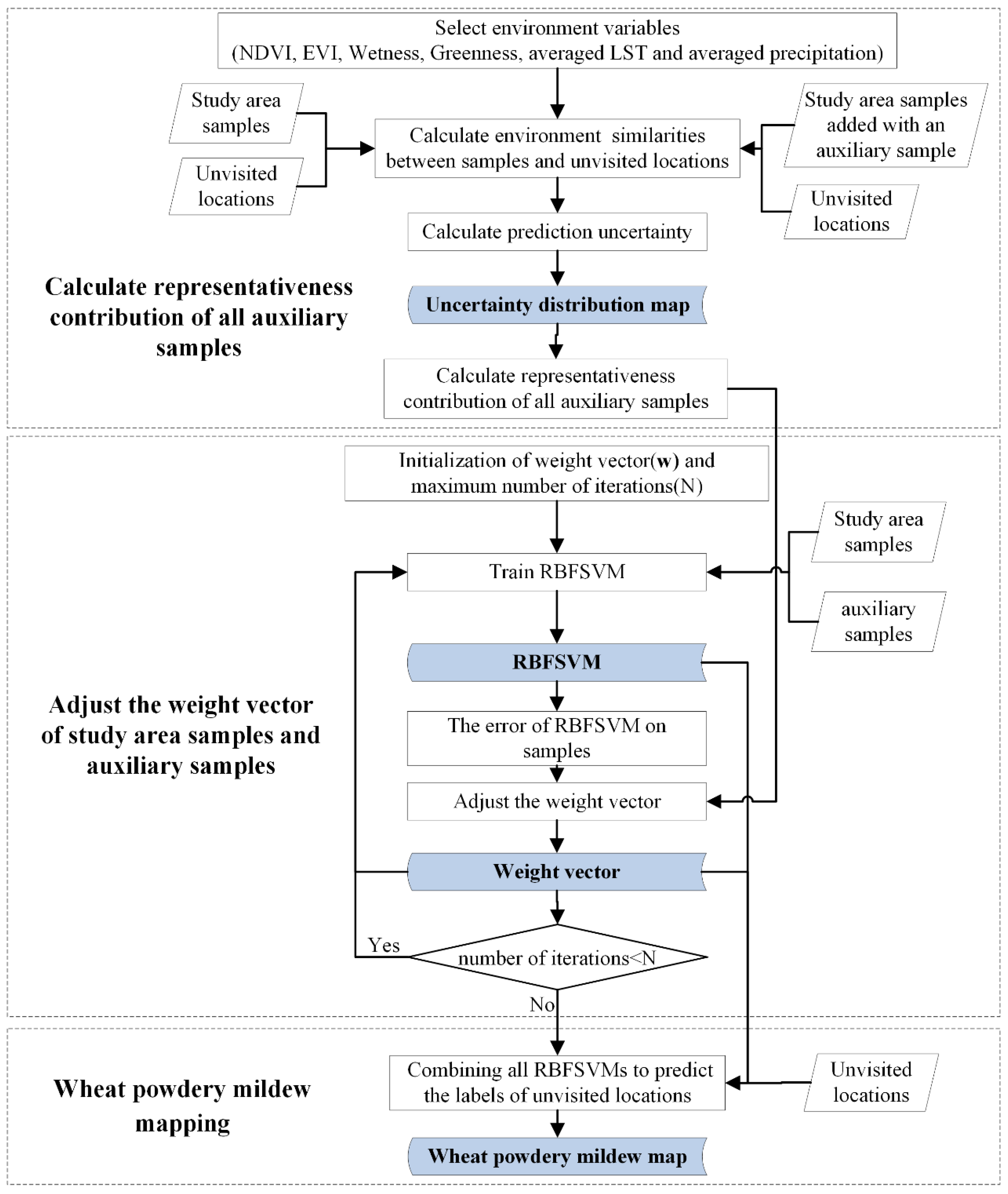
Since samples in this study were divided into three groups: health, slightly infected, and seriously infected, this algorithm needed to categorize instances precisely into one of the three classes. In our experiment, the multiclassification was achieved based on a one-versus-one approach [53]. We had trained three OpTrAdaBoost classifiers in the experiment; each classifier receives the samples of a pair of classes from the training dataset and learns to distinguish these two classes. When monitoring the wheat powdery mildew, a voting scheme is applied: all three OpTrAdaBoost classifiers were applied to an unvisited location and the class that got the highest number of votes got predicted. Figure 3 shows the flowchart of the overall methodology.

2.4. Existing Algorithms for Disease Monitoring

We selected five commonly used methods, the Mahalanobis distance (MD), partial least square regression (PLSR), Fisher’s linear discriminant analysis (FLDA), logistic regression (LR), and support vector machine (SVM), to compare with our algorithm OpTrAdaBoost. The existing methods are widely utilized to monitor disease outbreaks. The parameter settings used for SVM were exactly the same as those of OpTrAdaBoost, and

Table 3. Characteristics of existing methods used in this study for disease monitoring.

Methods	Full Name	Description	Literature
MD	Mahalanobis distance	A direction-sensitive distance classifier that uses statistics for each class and assumes all class covariances are equal.	Richards, 1999 [54]
PLSR	Partial least square regression	A statistical method that finds a linear regression model by projecting the predicted variables and the observable variables to a new space.	Herman, 1985 [55]
FLDA	Fisher’s linear discriminant analysis	A method used in statistics, pattern recognition, and machine learning to find a linear combination of features that characterizes or separates two or more classes of objects.	McLachlan, 2004 [56]
LR	Logistic regression	A statistical method that is used to describe the relationship between a dependent variable and multiple independent variables. It is less affected by some non-normality of variables.	David, 2010 [57]
SVM	Support vector machine	A supervised learning model that divides the examples of the separate categories by a clear gap that is as wide as possible.	Hearst, 1998 [58]

contains detailed descriptions of these methods.

3. Results

3.1. Influence of Parameters

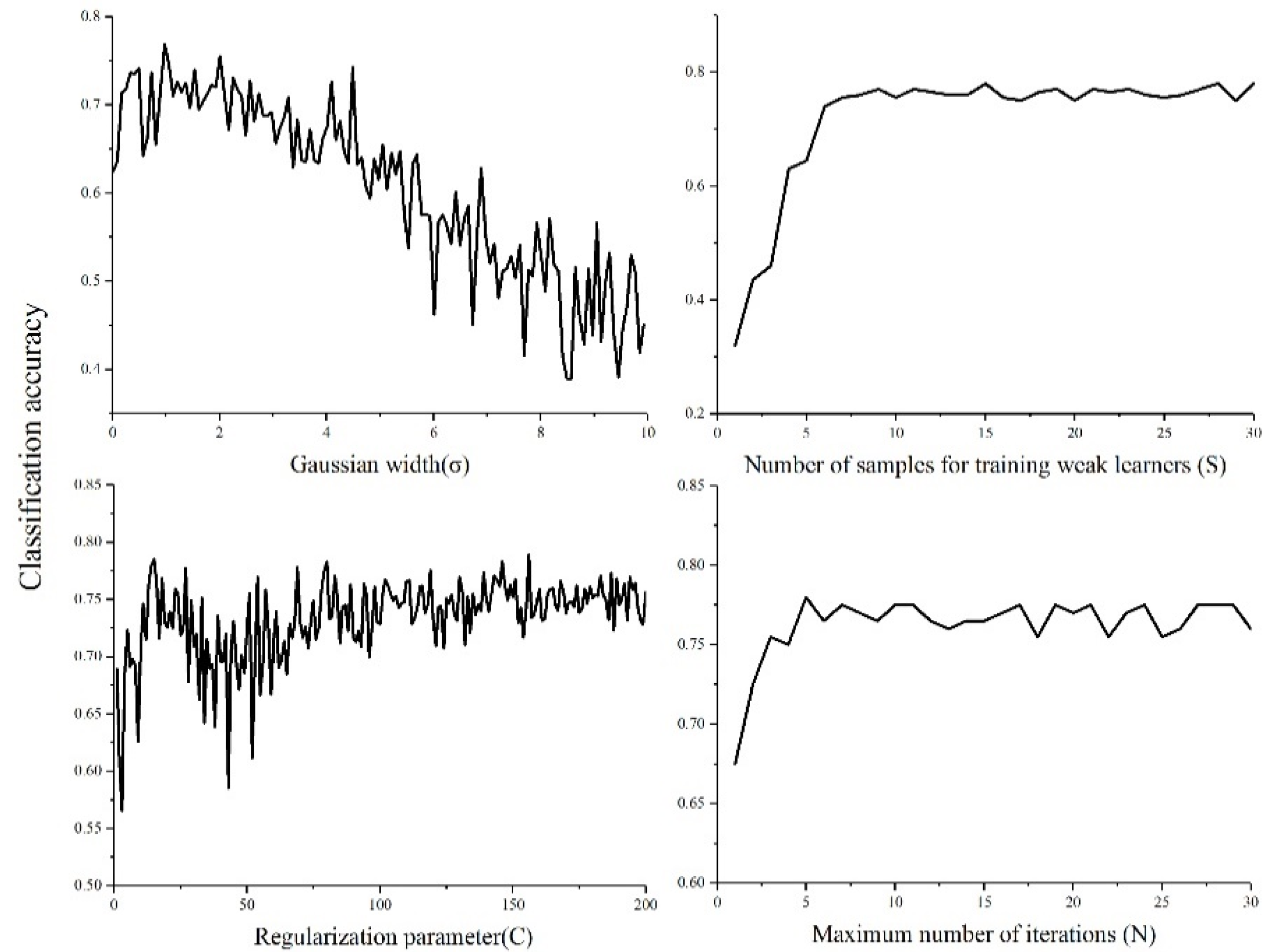
The performance of OpTrAdaBoost was affected by the Gaussian width (σ) of the RBFSVM, regularization parameter (C) of the RBFSVM, number of samples (S) used to train the RBFSVM per iteration, and maximum number of iterations (N). Classification results of OpTrAdaBoost were used to find suitable values for C, σ, N, and S. Since we did not have enough samples in the study area to partition it into training and test datasets, the leave-one-out cross validation was used to evaluate the generalization performance. The value of σ varied from σ_min to σ_max, where σ_min was the minimal Euclidean distance of all training samples in the input space and σ_max was the scatter radius of all training samples. The values of C, N, and S varied from 1 to 200, 1 to 50, and 1 to 65, respectively. For each variable, the experiment was repeated 10 times and the average accuracy was calculated (Figure 4). In general, the curve of each variable is a little noisy and it may have to do with the fact that the leave-one-out cross validation produces “noisy” (high-variance) results in general. Also, we observed that:

(1)

When C was small, variation of C led to some variation in the accuracy of disease classification. In general, the classification accuracy increased as C increased, and then the classification accuracy fell to 58%. After that, the classification accuracy increased again until it reached 0.75. In the end, the variation of C had little effect on the final generalization performance. One likely reason was that when N was fixed and C was increasing, the value of the loss function of the RBFSVM for samples that were predicted incorrectly became higher. This can lead to faster weight adjustment of the training instance, so that new samples had the chance to be chosen to train the weak learner. When all samples had been chosen to train the weak learners, the accuracy became stable.

(2)

The curve of σ was quite different from C, where a small bulge at the left top corner was observed, suggesting that the classification accuracy rose slightly until σ increased to a certain value. Then, the classification accuracy decreased gradually as σ increased. This suggests that the variation of σ has a larger impact on the final performance of OpTrAdaBoost compared to C.

(3)

S and N showed similar influence on OpTrAdaBoost. The classification accuracy increased quickly to the highest value and then became stable. However, the variation of S led to a larger change of classification accuracy than N before classification accuracy reached a “steady state”, suggesting that S has a stronger impact on the performance of OpTrAdaBoost than N.

3.2. Comparison of Different Algorithms

We compared OpTrAdaBoost with five existing algorithms using the leave-one-out cross validation to evaluate the general performance of these algorithms. First, we evaluated the classification accuracies of the five commonly used algorithms using two training datasets: a dataset consisting only of study area samples (T₁) and a dataset consisting of both auxiliary and study area samples (T₂) (

Table 4. The classification accuracy of five commonly used algorithms on two different training datasets.

Training Dataset	Algorithm
	FLDA	LR	MD	PLSR	SVM
T1	74%	67%	49%	59%	74%
T2	44%	54%	54%	49%	62%

), and the accuracy of classification varied significantly for different algorithms. On T₁, the overall accuracy varied from 49% to 74%, and on T₂, the overall accuracy varied from 44% to 62%. FLDA, LR, PLSR, and SVM yielded higher accuracy on T₁ than T₂; however, MD yielded higher accuracy on T₂ compared to T₁. Among the five commonly used algorithms, FLDA and SVM had the highest classification accuracy on T₁ (74%) and MD performed the worst on T₁ (49%). SVM produced the highest classification accuracy on T₂ (62%), and FLDA produced the worst performance on T₂ (44%).

We next compared the performance of OpTrAdaBoost on the T₂ dataset to the performances of the five commonly used algorithms on the T₁ dataset (

Table 5. Overall verification results of five commonly used algorithms and OpTrAdaBoost.

		Reference				User’s Accuracy (%)	Overall Accuracy (%)	Kappa
		Normal	Slight	Serious	Sum
FLDA	Normal	9	5	0	14	64	74	0.61
	Slight	2	11	0	13	85
	Serious	0	3	9	12	75
	Sum	11	19	9	39
	Producer’s accuracy (%)	82	58	100
	TP rate (%)	82	58	100
	Type I error	18	42	0
	TN rate (%)	82	90	90
	Type II error	18	10	10
LR	Normal	8	3	0	11	73	67	0.48
	Slight	3	12	3	18	67
	Serious	0	4	6	10	60
	Sum	11	19	9	39
	Producer’s accuracy (%)	73	63	67
	TP rate (%)	73	63	67
	Type I error	27	37	33
	TN rate (%)	89	70	87
	Type II error	11	30	13
MD	Normal	1	1	0	2	50	49	0.02
	Slight	10	18	9	37	49
	Serious	0	0	0	0	0
	Sum	11	19	9	39
	Producer’s accuracy (%)	9	95	0
	TP rate (%)	9	95	0
	Type I error	91	5	100
	TN rate (%)	96	5	100
	Type II error	4	95	0
PLSR	Normal	7	3	0	10	70	59	0.31
	Slight	4	14	7	25	56
	Serious	0	2	2	4	50
	Sum	11	19	9	39
	Producer’s accuracy (%)	64	74	22
	TP rate (%)	64	74	22
	Type I error	36	26	78
	TN rate (%)	89	45	93
	Type II error	11	55	7
SVM	Normal	9	2	0	11	82	74	0.59
	Slight	2	14	3	19	74
	Serious	0	3	6	9	67
	Sum	11	19	9	39
	Producer’s accuracy (%)	82	74	67
	TP rate (%)	82	74	67
	Type I error	18	26	33
	TN rate (%)	93	75	90
	Type II error	7	25	10
OpTrAdaBoost	Normal	10	3	1	14	71	82	0.72
	Slight	1	14	0	15	93
	Serious	0	2	8	10	80
	Sum	11	19	9	39
	Producer’s accuracy (%)	91	74	89
	TP rate (%)	91	74	89
	Type I error	9	26	11
	TN rate (%)	86	95	93
	Type II error	14	5	7

). We did not compare results of the T₂ dataset because the existing algorithms did not produce higher classification accuracy on the T₂ dataset. We found that the accuracy indices of the disease classifications varied significantly by algorithm, with overall accuracy ranging from 49% to 82% and the kappa coefficient ranging from 0.02 to 0.72 (Table 5). When comparing the six algorithms, OpTrAdaBoost performed better than the other algorithms.

The user’s accuracy and producer’s accuracy of slightly infected, heavily infected, and healthy classes reflected the commission error and omission error of each class (Table 5). For the healthy class, the user’s accuracy varied from 50% to 82% and producer’s accuracy varied from 9% to 91%. MD had lowest user’s accuracy and producer’s accuracy, which indicated that it performed worst in identifying healthy samples. OpTrAdaBoost produced the highest producer’s accuracy of 91%, and the user’s accuracy was 71%, indicating that OpTrAdaBoost was able to accurately identify healthy samples, but tended to misclassify diseased samples as healthy samples. For the slightly infected class, MD had the highest producer’s accuracy and lowest user’s accuracy, suggesting that too many healthy and seriously infected samples were misclassified as slightly infected samples when using MD. FLDA, LR, PLSR, and SVM yielded moderate accuracy for identifying the slightly infected class, and OpTrAdaBoost produced the highest user’s accuracy of 93%, and the producer’s accuracy was 74%, which indicated that it was able to accurately identify the slightly infected samples, but tended to misclassify slightly infected samples as samples of other classes. As for the seriously infected class, except for FLDA and OpTrAdaBoost, the other algorithms were unable to accurately identify the seriously infected samples, as was indicated by the less than 70% accuracy of the user and producer’s categorization of severely infected samples.

Additionally, all six methods had different capabilities in discriminating the three classes. MD performed poorly in classifying both healthy and diseased samples. PLSR yielded moderate accuracy for healthy samples, and low accuracies for slight and severe diseased samples. LR produced higher overall accuracy compared to PLSR, and it performed better when classifying both the healthy and diseased samples. SVM and FLDA had the same overall accuracy, while FLDA performed better in identifying the seriously infected samples. OpTrAdaBoost produced the highest overall accuracy and it is the only one algorithm that had over 70% user’s and producer’s accuracy for all three classes. Taken together, OpTrAdaBoost was superior in discriminating in healthy samples and the two levels of diseased samples.

3.3. Disease Mapping by OpTrAdaBoost

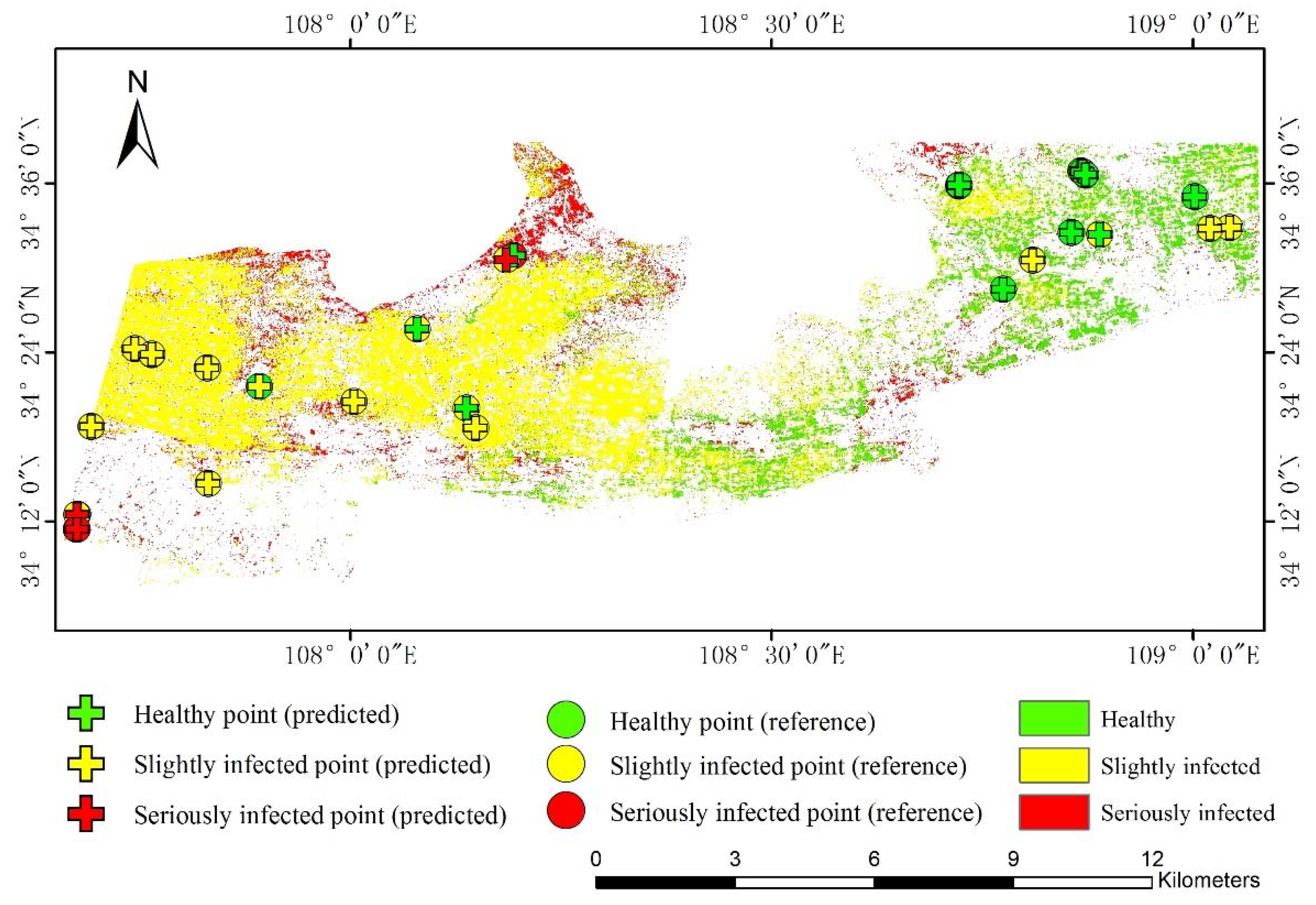
Using all features (NDVI, EVI, wetness, greenness, average LST, and average precipitation), the infection map of powdery mildew was produced using OpTrAdaBoost (Figure 5). In general, the Western region of the Western Guanzhong Plain had more infected areas and higher intensity of powdery mildew compared to the eastern region, which is in agreement with our field observations. A slightly infected area was located in the middle of the western region and seriously infected wheat were distributed along the Northwest and Southwest regions. To visually compare the estimated and the field infection data, samples were labeled with cross and circle signs in Figure 5. In the resulting map, a correct estimation of the model was indicated with data points that have the same color of the cross and circle sign. Overall, we found that most samples were correctly classified. However, the slightly infected samples tended to be misclassified as healthy, and seriously infected samples were often misclassified in the Northern region as slightly infected.

4. Discussion

Here, we found that the commonly used algorithms for monitoring crop disease were unable to produce higher classification accuracy on datasets consisting of both auxiliary and study area samples (see Section 3.2). The highest classification accuracy of the existing algorithms was 62% (Table 4) and the average accuracy was 50%. This indicates that while auxiliary data can be used to improve a model, it also introduces noise that can reduce the accuracy of the model. These algorithms do not have the ability to extract information from the auxiliary data and discard the noise, and this likely resulted in the low classification accuracy in these models when using auxiliary data.

We also found that the six algorithms (MD, PLSR, FLDA, LR, SVM, and OpTrAdaBoost) exhibited different traits in mapping the intensity of powdery mildew (Table 5). MD performed worse than the other methods and was unable to identify samples that were labeled as healthy and seriously infected. This may have been caused by the smaller sample size of healthy and seriously infected samples in our dataset, and the complex relationship between features (NDVI, EVI, wetness, greenness, average LST, and average precipitation) and severity of powdery mildew. LR and PLSR are commonly used algorithms for classification; however, their performance on our dataset was moderate. LR performed better than PLSR in identifying the healthy and seriously infected classes. This was likely caused by the PLSR’s use of principal components instead of original features to establish the relationship between raw data and disease severity [59,60], thus the model lost some information from the original data, which reduced its performance for monitoring disease. FLDA and SVM showed distinct characteristics in disease monitoring. FLDA performed well in discriminating seriously infected samples, with over 70% user’s and producer’s accuracy of the seriously infected class. The producer’s accuracy of FLDA was better than OpTrAdaBoost, and one likely reason was that OpTrAdaBoost also brought some noise when it extracted useful information from the auxiliary data. The noisy part of the seriously infected samples had more effect on the learner because the appearances of seriously infected samples in the study area and auxiliary area were different due to the difference in wheat cultivar. Despite this, FLDA performed poorly in differentiating the slightly infected class, and its high value for user’s accuracy and low value for producer’s accuracy for the slightly infected class indicated that FLDA overestimated the healthy and seriously infected areas to a certain degree. FLDA is a classical method for projecting high-dimensional feature vectors into a lower dimension through a linear transformation process that best separates the data groups [61]. However, the field samples of different classes were not always linearly separable, and FLDA does not perform well when the data is not linearly separable, which may explain its poor performance in differentiating the slightly infected class. In contrast, SVM performed better at identifying the slightly infected samples compared to FLDA. SVM can efficiently perform a nonlinear classification using the kernel trick, implicitly mapping the inputs into high-dimensional feature spaces, which may have resulted in its higher performance.

OpTrAdaBoost performed better than the exiting algorithms, especially in discriminating infected and noninfected regions. For the healthy class of samples, OpTrAdaBoost had producer’s accuracy over 90%, overall accuracy over 80%, and kappa over 0.7. OpTrAdaBoost was also better at discriminating slightly infected regions compared to the other algorithms, and its producer’s accuracy and user’s accuracy for the slightly infected class were 73% and 93%, respectively. The good performance of OpTrAdaBoost is likely due to two features. OpTrAdaBoost used RBFSVM as the weak learner in this study, thus it had the advantages of SVM to effectively avoid overfitting the data by selecting proper values of C and σ. In addition, OpTrAdaBoost also used auxiliary samples to monitor powdery mildew. By adjusting the weight placed on the auxiliary samples, the algorithm extracted useful information from the auxiliary data and used the additional information to improve the representativeness of study area samples, thus improving the quantity and quality of training data. For the seriously infected class, OpTrAdaBoost performed better than other algorithms except FLDA; future studies could synergize their traits and combine the two algorithms to improve the accuracy in discriminating serious instances from the others.

However, it should be noted that some limitations and challenges still remain in monitoring crop diseases with OpTrAdaBoost at a regional scale. Firstly, more factors, such as crop cultivars, cultivation procedures, management practices, etc., needed to be taken into consideration when choosing the auxiliary area to reduce the noise caused by these factors. Secondly, the field samples of the study area and auxiliary area were acquired at nearly the same time. Therefore, it is not clear whether OpTrAdaBoost will perform well when field samples are acquired at different times. In addition, some environmental variations, such as phenological difference, cultivation procedures, and soil types, may also cause some confusions and uncertainties in disease monitoring given their similar feature properties with disease. In future research, increased disease fieldwork with the above factors should be considered when generating models to monitor disease at regional scales in a reliable manner.

5. Conclusions

Monitoring of wheat powdery mildew at a regional level is of practical importance for agricultural management. In this study, we proposed an algorithm, OpTrAdaBoost, to monitor wheat powdery mildew in the Western Guanzhong Plain using auxiliary field data acquired from the suburban area of Shijiazhuang. From the dataset, a set of variables that can indicate crop growth status and environmental characteristics were extracted, and a monitoring model based on OpTrAdaBoost was developed. The performance of OpTrAdaBoost was compared to five commonly used algorithms. All algorithms showed different traits when mapping the intensity of powdery mildew, and OpTrAdaBoost performed the best among all algorithms. Our results suggest that the OpTrAdaBoost algorithm proposed in this study is able to produce a reasonable wheat powdery mildew damage map with an overall accuracy of 82%. Therefore, such a method could provide an economic and efficient alternative to conventional methods, especially in the regions where the collection of data is difficult. Future studies should try to evaluate the performance of OpTrAdaBoost when field samples are acquired at different times. Along with this, using more variables, such as soil type, crop cultivars, and so forth, to develop a more comprehensive model to monitor crop disease may help reduce the uncertainty level in the disease mapping process. Moreover, incorporating information of inoculum source and physical processing models (e.g., the Susceptible Infected Recovered Model (SIR Model)), which could describe the disease dispersal behavior and mechanism, will be expected to facilitate the disease monitoring process.

References

- Cao, X.; Luo, Y.; Zhou, Y.; Duan, X.; Cheng, D. Detection of powdery mildew in two winter wheat cultivars using canopy hyperspectral reflectance. Crop Prot. 2013, 45, 124–131. [Google Scholar] [CrossRef]
- Shen, X.K.; Ma, L.X.; Zhong, S.; Liu, N.; Zhang, M.; Chen, W.; Zhou, Y.; Li, H.J.; Chang, Z.J.; Li, X. Identification and genetic mapping of the putative Thinopyrum intermedium-derived dominant powdery mildew resistance gene PmL962 on wheat chromosome arm 2BS. Theor. Appl. Genet. 2015, 128, 517–528. [Google Scholar] [CrossRef] [PubMed]
- Zhang, J.; Pu, R.; Yuan, L.; Wang, J.; Huang, W.; Yang, G. Monitoring Powdery Mildew of Winter Wheat by Using Moderate Resolution Multi-Temporal Satellite Imagery. PLOS ONE 2014, 9. [Google Scholar] [CrossRef] [PubMed]
- Li, B.; Cao, X.; Chen, L.; Zhou, Y.; Duan, X.; Luo, Y.; Fitt, B.D.; Xu, X.; Song, Y.; Wang, B. Application of geographic information systems to identify the oversummering regions of Blumeria graminis f. sp. tritici in China. Plant Dis. 2013, 97, 1168–1174. [Google Scholar] [CrossRef]
- Shi, Y.; Huang, W.; Zhou, X. Evaluation of wavelet spectral features in pathological detection and discrimination of yellow rust and powdery mildew in winter wheat with hyperspectral reflectance data. J. Appl. Remote Sens. 2017, 11, 026025. [Google Scholar] [CrossRef]
- Yuan, L.; Bao, Z.; Zhang, H.; Zhang, Y.; Liang, X. Habitat monitoring to evaluate crop disease and pest distributions based on multi-source satellite remote sensing imagery. Optik Int. J. Light Electron. Opt. 2017, 145, 66–73. [Google Scholar] [CrossRef]
- Yuan, L.; Zhang, J.; Shi, Y.; Nie, C.; Wei, L.; Wang, J. Damage Mapping of Powdery Mildew in Winter Wheat with High-Resolution Satellite Image. Remote Sens. 2014, 6, 3611. [Google Scholar] [CrossRef]
- Mutanga, O.; Dube, T.; Galal, O. Remote sensing of crop health for food security in Africa: Potentials and constraints. Remote Sens. Appl. Soc. Environ. 2017, 8, 231–239. [Google Scholar] [CrossRef]
- Pryzant, R.; Ermon, S.; Lobell, D. Monitoring Ethiopian Wheat Fungus with Satellite Imagery and Deep Feature Learning. In Proceedings of the 2017 IEEE Conference on Computer Vision and Pattern Recognition Workshops (CVPRW), Honolulu, HI, USA, 21–26 July 2017; pp. 1524–1532. [Google Scholar]
- Luo, J.; Zhao, C.; Huang, W.; Zhang, J.; Zhao, J.; Dong, Y.; Yuan, L.; Du, S. Discriminating Wheat Aphid Damage Degree Using 2-Dimensional Feature Space Derived from Landsat 5 TM. Sens. Lett. 2012, 10, 608–614. [Google Scholar] [CrossRef]
- Bauriegel, E.; Giebel, A.; Geyer, M.; Schmidt, U.; Herppich, W.B. Early detection of Fusarium infection in wheat using hyper-spectral imaging. Comput. Electron. Agric. 2011, 75, 304–312. [Google Scholar] [CrossRef]
- Bhattacharya, B.K.; Chattopadhyay, C. A multi-stage tracking for mustard rot disease combining surface meteorology and satellite remote sensing. Comput. Electron. Agric. 2013, 90, 35–44. [Google Scholar] [CrossRef]
- Huang, W.; Guan, Q.; Luo, J.; Zhang, J.; Zhao, J.; Liang, D.; Huang, L.; Zhang, D. New Optimized Spectral Indices for Identifying and Monitoring Winter Wheat Diseases. IEEE J. Sel. Top. Appl. Earth Obs. Remote Sens. 2014, 7, 2516–2524. [Google Scholar] [CrossRef]
- Luo, J.; Huang, W.; Zhao, J.; Zhang, J.; Ma, R.; Huang, M. Predicting the probability of wheat aphid occurrence using satellite remote sensing and meteorological data. Optik Int. J. Light Electron. Opt. 2014, 125, 5660–5665. [Google Scholar] [CrossRef]
- Shi, Y.; Huang, W.; Luo, J.; Huang, L.; Zhou, X. Detection and discrimination of pests and diseases in winter wheat based on spectral indices and kernel discriminant analysis. Comput. Electron. Agric. 2017, 141, 171–180. [Google Scholar] [CrossRef]
- Nie, C.; Yuan, L.; Yang, X.; Wei, L.; Yang, G.; Zhang, J. Comparison of Methods for Forecasting Yellow Rust in Winter Wheat at Regional Scale. IFIP Adv. Inf. Commun. Technol. 2015, 452, 444–451. [Google Scholar] [CrossRef]
- Chemura, A.; Mutanga, O.; Dube, T. Separability of coffee leaf rust infection levels with machine learning methods at Sentinel-2 MSI spectral resolutions. Precis. Agric. 2016, 18, 859–881. [Google Scholar] [CrossRef]
- Jin, X.; Jie, L.; Wang, S.; Qi, H.; Li, S. Classifying Wheat Hyperspectral Pixels of Healthy Heads and Fusarium Head Blight Disease Using a Deep Neural Network in the Wild Field. Remote Sens. 2018, 10, 395. [Google Scholar] [CrossRef]
- Chan, C.S.; Anderson, D.T.; Ball, J.E. Comprehensive survey of deep learning in remote sensing: Theories, tools, and challenges for the community. J. Appl. Remote Sens. 2017, 11, 1. [Google Scholar] [CrossRef]
- Lv, J.-J.; Shao, X.-H.; Huang, J.-S.; Zhou, X.-D.; Zhou, X. Data augmentation for face recognition. Neurocomputing 2017, 230, 184–196. [Google Scholar] [CrossRef]
- Grinias, I.; Panagiotakis, C.; Tziritas, G. MRF-based segmentation and unsupervised classification for building and road detection in peri-urban areas of high-resolution satellite images. ISPRS J. Photogramm. Remote Sens. 2016, 122, 145–166. [Google Scholar] [CrossRef]
- Leichtle, T.; Geiß, C.; Lakes, T.; Taubenböck, H. Class imbalance in unsupervised change detection—A diagnostic analysis from urban remote sensing. Int. J. Appl. Earth Obs. Geoinf. 2017, 60, 83–98. [Google Scholar] [CrossRef]
- Tuia, D.; Persello, C.; Bruzzone, L. Domain adaptation for the classification of remote sensing data: An overview of recent advances. IEEE Geosci. Remote Sens. Mag. 2016, 4, 41–57. [Google Scholar] [CrossRef]
- Pan, S.J.; Yang, Q. A survey on transfer learning. IEEE Trans. Knowl. Data Eng. 2010, 22, 1345–1359. [Google Scholar] [CrossRef]
- Othman, E.; Bazi, Y.; Alajlan, N.; Alhichri, H.; Melgani, F. Using convolutional features and a sparse autoencoder for land-use scene classification. Int. J. Remote Sens. 2016, 37, 2149–2167. [Google Scholar] [CrossRef]
- Ghazi, M.M.; Yanikoglu, B.; Aptoula, E. Plant identification using deep neural networks via optimization of transfer learning parameters. Neurocomputing 2017, 235, 228–235. [Google Scholar] [CrossRef]
- Ma, Y.; Gong, W.; Mao, F. Transfer learning used to analyze the dynamic evolution of the dust aerosol. J. Quant. Spectrosc. Radiat. Transf. 2015, 153, 119–130. [Google Scholar] [CrossRef]
- Lv, X.; Yi, G.; Deng, B. Transfer learning based clinical concept extraction on data from multiple sources. J. Biomed. Inf. 2014, 52, 55–64. [Google Scholar] [CrossRef] [Green Version]
- Li, N.; Hao, H.; Gu, Q.; Wang, D.; Hu, X. A transfer learning method for automatic identification of sandstone microscopic images. Comput. Geosci. 2017, 103, 111–121. [Google Scholar] [CrossRef]
- Ma, H.; Jing, Y.; Huang, W.; Shi, Y.; Dong, Y.; Zhang, J.; Liu, L. Integrating Early Growth Information to Monitor Winter Wheat Powdery Mildew Using Multi-Temporal Landsat-8 Imagery. Sensors 2018, 18. [Google Scholar] [CrossRef]
- Bai, J.-J.; Yu, Y.; Di, L. Comparison between TVDI and CWSI for drought monitoring in the Guanzhong Plain, China. J. Integr. Agric. 2017, 16, 389–397. [Google Scholar] [CrossRef]
- Li, S.; Li, Y.; Li, X.; Tian, X.; Zhao, A.; Wang, S.; Wang, S.; Shi, J. Effect of straw management on carbon sequestration and grain production in a maize–wheat cropping system in Anthrosol of the Guanzhong Plain. Soil Tillage Res. 2016, 157, 43–51. [Google Scholar] [CrossRef]
- Zhou, J.; Zhang, Y.; Zhou, A.; Liu, C.; Cai, H.; Liu, Y. Application of hydrochemistry and stable isotopes (δ34S, δ18O and δ37Cl) to trace natural and anthropogenic influences on the quality of groundwater in the piedmont region, Shijiazhuang, China. Appl. Geochem. 2016, 71, 63–72. [Google Scholar] [CrossRef]
- Niu, J.; Zhang, W.; Ru, S.; Chen, X.; Xiao, K.; Zhang, X.; Assaraf, M.; Imas, P.; Magen, H.; Zhang, F. Effects of potassium fertilization on winter wheat under different production practices in the North China Plain. Field Crops Res. 2013, 140, 69–76. [Google Scholar] [CrossRef]
- Funk, C.C.; Peterson, P.J.; Landsfeld, M.F.; Pedreros, D.H.; Verdin, J.P.; Rowland, J.D.; Romero, B.E.; Husak, G.J.; Michaelsen, J.C.; Verdin, A.P. A Quasi-Global Precipitation Time Series for Drought Monitoring; 2327-638X; US Geological Survey: Reston, VA, USA, 2014.
- Chander, G.; Markham, B.L.; Helder, D.L. Summary of current radiometric calibration coefficients for Landsat MSS, TM, ETM+, and EO-1 ALI sensors. Remote Sens. Environ. 2009, 113, 893–903. [Google Scholar] [CrossRef] [Green Version]
- Pacifici, F.; Longbotham, N.; Emery, W.J. The Importance of Physical Quantities for the Analysis of Multitemporal and Multiangular Optical Very High Spatial Resolution Images. IEEE Trans. Geosci. Remote Sens. 2014, 52, 6241–6256. [Google Scholar] [CrossRef]
- Wan, Z.; Dozier, J. A generalized split-window algorithm for retrieving land-surface temperature from space. IEEE Trans. Geosci. Remote Sens. 1996, 34, 892–905. [Google Scholar]
- Zou, Y.-F.; Qiao, H.-B.; Cao, X.-R.; Liu, W.; Fan, J.-R.; Song, Y.-L.; Wang, B.-T.; Zhou, Y.-L. Regionalization of wheat powdery mildew oversummering in China based on digital elevation. J. Integr. Agric. 2018, 17, 901–910. [Google Scholar] [CrossRef]
- Liu, N.; Lei, Y.; Gong, G.; Zhang, M.; Wang, X.; Zhou, Y.; Qi, X.; Chen, H.; Yang, J.; Chang, X.; et al. Temporal and spatial dynamics of wheat powdery mildew in Sichuan Province, China. Crop Prot. 2015, 74, 150–157. [Google Scholar] [CrossRef]
- Gao, X.; Huete, A.R.; Ni, W.; Miura, T. Optical–biophysical relationships of vegetation spectra without background contamination. Remote Sens. Environ. 2000, 74, 609–620. [Google Scholar] [CrossRef]
- Pang, G.; Wang, X.; Yang, M. Using the NDVI to identify variations in, and responses of, vegetation to climate change on the Tibetan Plateau from 1982 to 2012. Quat. Int. 2017, 444, 87–96. [Google Scholar] [CrossRef]
- Xue, J.; Su, B. Significant remote sensing vegetation indices: A review of developments and applications. J. Sens. 2017, 2017. [Google Scholar] [CrossRef]
- Yuan, L.; Pu, R.; Zhang, J.; Wang, J.; Yang, H. Using high spatial resolution satellite imagery for mapping powdery mildew at a regional scale. Precis. Agric. 2015, 17, 332–348. [Google Scholar] [CrossRef]
- Liu, H.Q.; Huete, A. A feedback based modification of the NDVI to minimize canopy background and atmospheric noise. IEEE Trans. Geosci. Remote Sens. 1995, 33, 457–465. [Google Scholar]
- Miura, T. Overview of the radiometric and biophysical performance of the MODIS vegetation indices. Remote Sens. Environ. 2002, 83, 195–213. [Google Scholar]
- Dai, W.; Yang, Q.; Xue, G.-R.; Yu, Y. Boosting for transfer learning. In Proceedings of the 24th International Conference on Machine Learning, Corvalis, OR, USA, 20–24 June 2007; pp. 193–200. [Google Scholar]
- Boser, B.E.; Guyon, I.M.; Vapnik, V.N. A training algorithm for optimal margin classifiers. In Proceedings of the Fifth Annual Workshop on Computational Learning Theory, Pittsburgh, PA, USA, 27–29 July 1992; pp. 144–152. [Google Scholar]
- Scholkopf, B.; Sung, K.K.; Burges, C.J.C.; Girosi, F.; Niyogi, P.; Poggio, T.; Vapnik, V. Comparing support vector machines with Gaussian kernels to radial basis function classifiers. IEEE Trans. Signal Process. 1997, 45, 2758–2765. [Google Scholar] [CrossRef]
- Zhu, A.X.; Liu, J.; Du, F.; Zhang, S.J.; Qin, C.Z.; Burt, J.; Behrens, T.; Scholten, T. Predictive soil mapping with limited sample data. Eur. J. Soil Sci. 2015, 66, 535–547. [Google Scholar] [CrossRef] [Green Version]
- McBratney, A.B.; Santos, M.M.; Minasny, B. On digital soil mapping. Geoderma 2003, 117, 3–52. [Google Scholar] [CrossRef]
- Maskey, R.; Fei, J.; Nguyen, H.-O. Use of exploratory factor analysis in maritime research. Asian J. Shipp. Logist. 2018, 34, 91–111. [Google Scholar] [CrossRef]
- Zhang, Z.L.; Luo, X.G.; García, S.; Tang, J.F.; Herrera, F. Exploring the effectiveness of dynamic ensemble selection in the one-versus-one scheme. Knowl.-Based Syst. 2017, 125, 53–63. [Google Scholar] [CrossRef]
- Richards, J.; Jia, X. Remote Sensing Digital Image Analysis; Springer: Berlin, Germany, 1999. [Google Scholar]
- Wold, H. Partial least squares. In Encyclopedia of Statistical Sciences; Wiley: New York, NY, USA, 1985. [Google Scholar]
- McLachlan, G. Discriminant Analysis and Statistical Pattern Recognition; John Wiley & Sons: Hoboken, NJ, USA, 2004; Volume 544. [Google Scholar]
- Wooff, D.; Chevalier, A.; Sharples, L. Logistic Regression: A Self-learning Text, 2nd ed.; Springer: Berlin, Germany, 2010; pp. 192–194. [Google Scholar]
- Hearst, M.A.; Dumais, S.T.; Osuna, E.; Platt, J.; Scholkopf, B. Support vector machines. IEEE Intell. Syst. Appl. 1998, 13, 18–28. [Google Scholar] [CrossRef]
- Li, B.; Morris, J.; Martin, E.B. Model selection for partial least squares regression. Chemom. Intell. Lab. Syst. 2002, 64, 79–89. [Google Scholar] [CrossRef]
- Faber, N.; Rajko, R. How to avoid over-fitting in multivariate calibration—The conventional validation approach and an alternative. Anal. Chim. Acta 2007, 595, 98–106. [Google Scholar] [CrossRef] [PubMed]
- AbuZeina, D.; Al-Anzi, F.S. Employing fisher discriminant analysis for Arabic text classification. Comput. Electr. Eng. 2017. [Google Scholar] [CrossRef]
Figure 1.
The location and sampling sites of the two areas: Western Guanzhong Plain (left) and suburban farmlands of Shijiazhuang (right). Yellow dots indicate locations that were sampled for wheat powdery mildew.
Figure 2.
A general overview of the results that can be obtained from the proposed algorithm, highlighting the auxiliary samples with different representativeness contributions and different similarities to study area samples.
Figure 3.
The flowchart of OpTrAdaBoost. RBFSVM: support vector machine with radial basis function kernel.
Figure 4.
The performance of OpTrAdaBoost with different values of σ, C, N, and S for the RBFSVM.
Figure 5.
The infection map of powdery mildew in Western Guanzhong Plain produced by OpTrAdaBoost. Green represents estimated healthy wheat, yellow represents estimated slightly infected wheat, and red represents estimated seriously infected wheat. Green circles are healthy samples, yellow circles are slightly infected samples, and red circles are seriously infected samples. Green crosses are estimated healthy wheat at the location of samples, yellow crosses are estimated slighted infected wheat at the location of samples, and red crosses are estimated seriously infected wheat at the location of samples.