Assimilating Remote Sensing Phenological Information into the WOFOST Model for Rice Growth Simulation

Abstract

Precise simulation of crop growth is crucial to yield estimation, agricultural field management, and climate change. Although assimilation of crop model and remote sensing data has been applied in crop growth simulation, few studies have considered optimizing the crop model with respect to phenology. In this study, we assimilated phenological information obtained from Moderate Resolution Imaging Spectroradiometer (MODIS) time series data into the World Food Study (WOFOST) model to improve the accuracy of rice growth simulation at the regional scale. The particle swarm optimization (PSO) algorithm was implemented to optimize the initial phenology development stage (IDVS) and transplanting date (TD) in the WOFOST model by minimizing the difference between simulated and observed phenology, including heading and maturity date. Assimilating phenology improved the accuracy of the rice growth simulation, with correlation coefficients (R) equal to 0.793, 0822, and 0.813 at three fieldwork dates. The performance of the proposed strategy is comparable with that of the enhanced vegetation index (EVI) time series assimilation strategy, with less computation time. Additionally, the result confirms that the proposed strategy could be applied with different spatial resolution images and the difference of simulated LAI_mean is less than 0.35 in three experimental areas. This study offers a novel assimilation strategy with regard to the phenology development process, which is efficient and scalable for crop growth simulation.

1. Introduction

Accurate crop growth simulation is important for crop yield prediction, field management, and climate change evaluation [1,2,3]. A crop growth model could quantify crop physiological development growth and yield based on the interactions among environmental characteristics (such as soil, weather, and water) [4,5,6]. The WOFOST model is one of the widely used crop model, which has been successfully applied at the field scale in previous studies [7,8]. However, the performance of this model is limited by the uncertainties of the initial parameters and an incomplete description of the simulation structure [9]. For example, physiological processes (such as photosynthesis and respiration) in the WOFOST model are strongly related to the phenology development process [4] and affected by input parameters and model initialization. Hence, the accuracy of the WOFOST model is expected to be improved with accurate initial parameters [10], especially for large-scale application.

The remote sensing technique is a cost-efficient approach for crop growth monitoring over large areas, which could reflect actual crop growth condition during the growth season. The geophysical scale could be extended by the combination of satellite data and the crop growth model [11]. Meanwhile, satellite data can be regarded as a “real” crop observation to constrain the crop model, thereby providing an accurate simulation result. Therefore, data assimilation, which incorporates observed data into dynamic mechanistic models, has been widely used in agricultural monitoring studies [12,13,14,15,16,17,18]. Ines et al. assimilated satellite-based soil moisture and leaf area index (LAI) into a crop model for maize yield estimation and indicated that the prediction performance in the assimilation-crop framework was improved compared to that without assimilation [14]. According to previous studies, the state variables in the assimilation can be divided into two types: Vegetation indices (such as normalized difference vegetation index, NDVI) and crop biophysical parameters (such as LAI, the fraction of absorbed photosynthetically active radiation (FAPAR), and surface soil moisture). The former combined the radiation transfer model and crop model to minimize the difference between model-simulated and satellite-observed vegetation indices through optimizing model initial parameters [19,20]. Liu et al. assimilated the NDVI into the PROSAIL-WOFOST coupled model to simulate rice growth [16]. However, some parameters (e.g., leaf angle distribution) in the radiation transfer model are constants, which is inconsistent with reality, leading to uncertainties. Biophysical parameters were increasingly applied in the assimilation, since they are significant at the crop growth stage and can be obtained from both the crop model and remote sensing data [6]. Most studies employed satellite-retrieved LAI as the state variable to optimize the crop model for various applications [21,22,23]. Nevertheless, the LAI retrieval typically relies on empirical models, which is resource intensive in terms of time and labor [24]. The empirical parameters in the model vary with crop types, time periods, and geophysical conditions [6]. Meanwhile, the selection of LAI data affects the assimilation results. Li et al. demonstrated that LAI in different phenological stages, temporal frequencies, and spatial scales influenced the accuracy of wheat yield estimation [21]. Additionally, although the large number of satellite images in the assimilation could improve the simulation accuracy, the computational burden inevitably increases, causing low assimilation efficiency, especially in a large area [25,26].

The development of crop phenology is an indispensable part of crop models (such as the WOFOST, CERES, and ORYZA models) since phenological information affects crop matter distribution during the growing stages [6,27]. Phenology is an intuitive representation of crop growth, reflecting crop periodic biological changes affected by the climate and other environmental conditions [28]. However, few studies have optimized crop growth simulation regarding the development of crop phenology. Taking the WOFOST model as an example, the model assumes crop growth starts from the emergence stage, but for rice, growth starts from the transplant stage in farmland [29,30]. Therefore, enhancing the process of phenology development in crop models is significant for crop growth simulation, especially for rice. Additionally, an increasing number of studies have indicated that the remote sensing technique provides more potential for accurate quantitative crop phenology monitoring [31,32]. Liu et al. extracted rice phenology from MODIS time series data to improve the accuracy of rice mapping [33]. Hence, it is feasible to assimilate satellite-derived phenological information into the crop model for crop growth simulation. Compared with directly assimilating satellite time series data, assimilating phenology extracted from time series data could lessen the computational burden since only a few images are input into the assimilation. Meanwhile, phenology is extracted from satellite time series data without empirical relationships, which is applicable across spatial and temporal domains [28,31].

In this study, we attempted to optimize the WOFOST model from the perspective of phenology development using satellite data. The MODIS EVI time-series product was adopted to extract the rice phenological stages (including transplanting, heading, and maturity). This phenological information was then assimilated into the WOFOST model through optimization of the initial phenology development stage (IDVS) and transplanting date (TD) to improve the model performance. Meanwhile, the Landsat 8 time series data was employed to verify the scalability of the proposed framework, with a spatial resolution of 30 m. We also assimilated the EVI time series data into the PROSAIL-WOFOST model for comparison.

2. Study Area and Data

2.1. Study Area

The study area is located in the Dongting Lake region in the northwest of Yueyang city, Hunan province, China, which is an important production base (Figure 1). The lake area is an alluvial plain with an elevation of 34 m [34]. The main land use type of the study area is cropland, specifically, paddy fields [35]. The rice cultivation is mainly single-season. This region belongs to the subtropical monsoon humid climate with sufficient sunshine for growing paddy rice from May to September. The average temperature ranges from 23 °C to 29.1 °C in summer. The annual precipitation ranges from 1100 to 1400 mm, and most of the precipitation occurs from April to June. Twenty points were selected in the study area for experimental sampling.

2.2. Field Data

The filed datasets include meteorological data and field-measured data. The meteorological data, including daily maximum and minimum temperatures, solar radiation, wind speed, actual vapor pressure, and precipitation, were downloaded from the China Meteorological Data Sharing Service System (http://data.cma.cn/) and used to drive the crop growth model. For Hunan province, there are 85 weather stations for calculation of meteorological data by an interpolation method.

Canopy LAI is collected during the entire rice growth season to validate the WOFOST model in the study region. Three fieldworks were conducted on 23 July, 8 August, and 23 August for collecting canopy LAI of rice. In the study area, 20 randomly distributed sampling plots were selected for field measurement. The locations were recorded with the global positioning system (GPS). Each sample site approximately covered an area of 250 m × 250 m, with five subplots enclosed in each site (Figure 1). Then, no-destructive LAI was measured five times in each 10 m × 10 m area around each subplot using the LAI-2000 LAI meter (LI-COR, Lincoln, NE, USA) in three fieldworks. The average of five times represents the subplot LAI value. Then LAI values from the five subplots were averaged to represent the unique LAI in each sample plot. Meanwhile, the samples of soil were collected in each sample plot and analyzed to obtain the profile of soil in the study area at the Chinese Academy of Agricultural Sciences [36].

2.3. Remote Sensing Data

GFSAD30AUNZCNMOCE data from USGS (https://web.croplands.org/) was downloaded for rice field extraction in this study. The data was processed for cropland classification with Landsat 8 time series images in 2015, with a spatial resolution of 30 m (Figure 1).

MODIS vegetation indices (VIs) products, including Terra MOD13Q1 data and Aqua MYD13Q1 data, were employed to extract the phenology information. For each product, the highest quality observations were selected over a 16-day period with respect to cloud state, aerosol quantity, observation coverage, and view angle. Since the start period of Terra and Aqua are DOY 001 and DOY 009, respectively, the combination of these two products could provide NDVI and EVI data with a temporal (spatial) resolution of 8-day (250 m). Both products have two quality assessment (QA) band (VI quality and pixel reliability) and for a detailed description of quality flags refer to [37]. In this study, pixels with good quality (rank 0) were directly selected based on the pixel reliability band. If the pixel was “marginal data” (rank 1), only pixels with no cloud, no shadow, and low aerosol were selected from the VI quality band. All appropriate satellite images were obtained in the rice growth period (May 15 to October 1 in 2017). In this study, the rice farmland was extracted based on cropland data and three extracted phenological dates derived from the MODIS time series [13]. The reasonable range of three rice phenology periods derived from the meteorological bureau (http://www.hnqx.gov.cn) and local farmers.

For an examination of the scalability of the proposed method, all available Landsat 8 surface reflectance images (30 m) from May 15th to October 1st in 2017 were downloaded from USGS archive (http://www.hnagri.gov.cn). Due to the cloudy effect and low temporal resolution (16 days), these images could not form valid EVI time series for phenology extraction in the entire study area. However, based on the cloud mask and visual interpretation, three small areas, located in the overlapped area among different paths and rows, could form EVI time series, which consequently were selected for an assessment of the scalability (marked by the black box in Figure 1b).

3. Methods

In this study, phenological information was extracted from MODIS time series data. Then, we assimilated the heading and maturity date into the WOFOST model through adjustment of IDVS and TD to optimize the rice growth simulation. Figure 2 shows the flowchart of the main methodology applied in this study. Meanwhile, the EVI time series data was assimilated into the PROSAIL-WOFOST model for comparison. The detailed information can be seen in the Supplementary Materials.

3.1. Phenology Development Simulation in the WOFOST Model

The WOFOST model is a dynamic and carbon-driven crop growth model, developed by the school of C.T. de Wit [5], which has a complex hierarchical structure. Diepen et al. [38] describes the details of the WOFOST model quite thoroughly in his study. Thus, only a brief introduction is presented in this paper regarding the phenology development simulation of the WOFOST model.

The process of phenology development in the WOFOST model is described by the dimensionless state variable development stage (DVS). For most annual crops, DVS is set to 0 at seedling emergence, 1 at flowering, and 2 at maturity. The determination of DVS depends on the accumulation of the daily development rate (DVR), which is a crop specific function of the surrounding temperature and is possibly affected by the photoperiod. Thermal time accumulation (sometimes called temperature sum or heat sum) is introduced to calculate DVR, which is proposed to reflect the effect of temperature on the development rate.

Thermal time accumulation is the integral over time of the daily effective temperature ($T_e$) after crop emergence. $T_e$ is the difference between the daily average temperature ($\mathrm{T}$) and a base temperature ($T_{base}$) below which no development occurs, i.e., $T_e=\max \left(\left(T-T_{base}\right),0\right)$. Above a certain maximum effective temperature $(T_{max-e})$, $T_e$ remains constant. Between $T_{max,e}$ and $T_{base}$, the daily increase in thermal time is obtained by linear interpolation. Then, DVR is calculated by $T_e$ [°C] and the required thermal time passing to the next development stage, $T_{req}$ [°C] (Equation (1)):

$$\mathrm{DVR}=\frac{T_e}{T_{req}}$$

(1)

In Equation (1), $T_{req}$ means the sum of the effective temperature between emergence to flowering or flowering to maturity, which needs a specific phenology transfer date for calculation. For transplanted rice, the transplant and heading stage represent the start and peak during rice growth in a paddy field, but the flowering stage is difficult identify since this stage is short. Therefore, we modified the definition of $T_{req}$ to “the sum of effective temperature between transplant to heading or heading to maturity”. The DVS values were reset correspondingly, with 1 for heading and 2 for maturity stage.

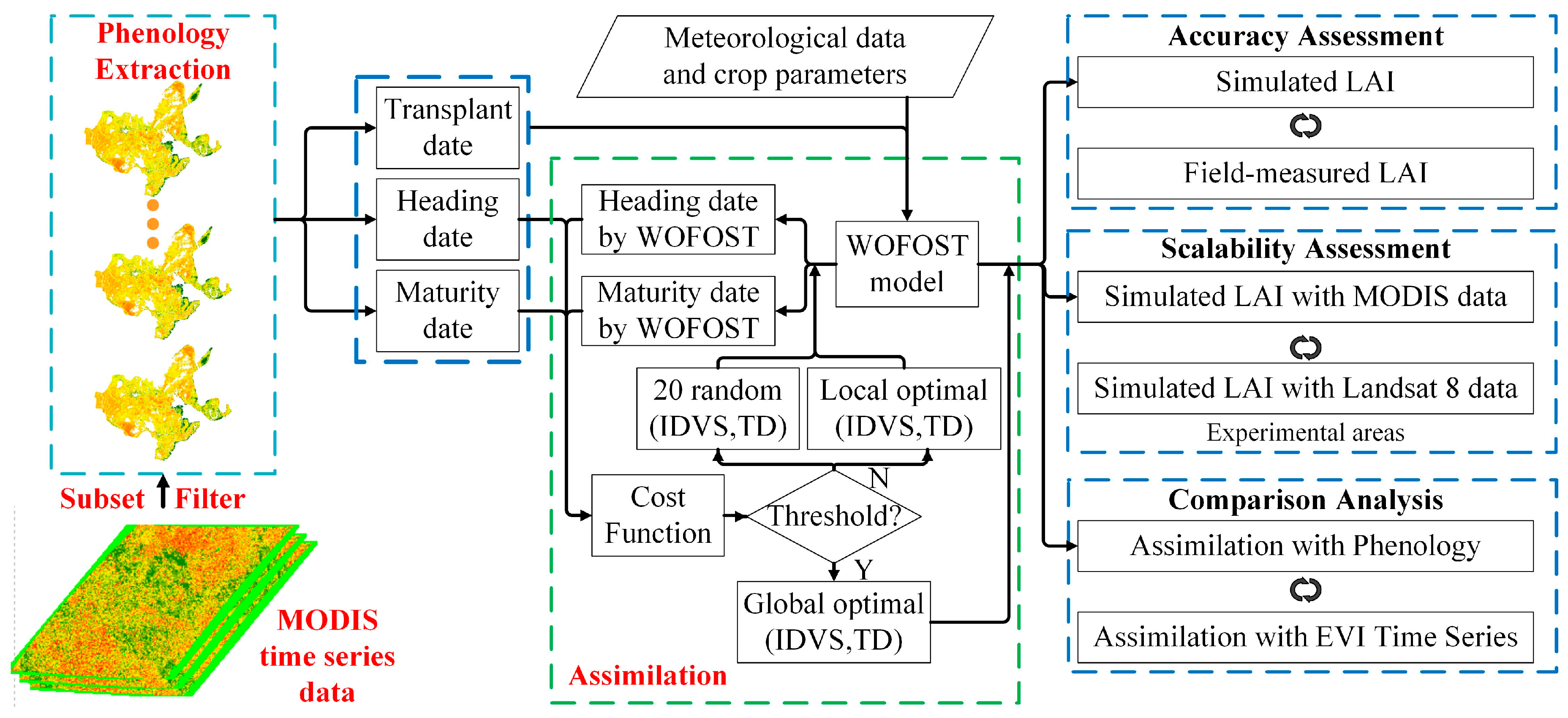
3.2. Phenology Extraction from Remote Sensing Data

The extraction of vegetation phenological information with satellite data is mostly based on the time series VIs. Therefore, it is crucial to select VIs that are sensitive to vegetation seasonal characteristics. NDVI and EVI have been proven to be the ideal indicators for vegetation status monitoring, thus they are widely used in phenology extraction studies [39,40,41]. The two VIs can reflect the comprehensive crop growth condition affected by the environment. However, NDVI is easily saturated in high vegetation coverage and affected by soil background. However, EVI could overcome the influence of soil background with the “anti-atmospheric vegetation index” and “anti-soil vegetation index” [42]. In this study, rice was transplanted in the early growth period, during which the crop coverage is low and soil background will easily affect the NDVI calculation. Therefore, we selected EVI from MODIS products to construct the EVI time series curve.

Although quality control has been conducted on MODIS composite products, the composite algorithm has not yet completely eliminated the effects caused by cloud, illumination, and topography. These factors result in the EVI time series data containing noise and thus affecting the accuracy of phenology extraction. Hence, the filtering method is applied to remove the noise and reconstruct the EVI time series. The Savitzky–Golay (S-G) smoothing filter, also known as the least squares or digital smoothing polynomial, is widely used to smooth the noise signal in phenology studies [43,44]. Therefore, S-G filtering was conducted to smooth the irregular EVI time series in this study, based on its locally adaptive moving window, which could keep the subtle local change of time-series data.

After smoothing, the rice growth cycle can be reflected by EVI time series curves. As the heading date is the peak of the growth period, rice also has maximum EVI values and cover fractions in remote sensing images [27,45]. In general, the rice field is flooded before transplanting and low EVI values are observed during this period [40]. However, with the transplanting of rice, the EVI values will increase. Therefore, it is reasonable to define the transplanting date of rice as the minimal point along the EVI profile. The EVI curve begins to decrease after the heading stage due to the etiolation and senescence of the rice leaves. The maturation date of rice is then identified by the minimum point in the first derivative of the EVI curve [46,47].

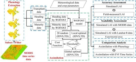
3.3. Assimilation of Remote Sensing Phenological Information with the WOFOST Model

The phenological parameters of the WOFOST model are generally acquired by fieldwork. However, fieldwork is not only inefficient, but also difficult to conduct on a regional scale. Therefore, remote sensing time series data are selected to extract the phenology transformation date. For rice, IDVS (DVS value at the date of transplanting) is determined by the growth condition before transplanting, instead of setting it as zero for other crops. Therefore, the IDVS was adjusted in the assimilation according to the effect of IDVS on rice growth simulation (Table S2). Additionally, low canopy cover fraction leads to high bias in the TD extraction, therefore, TD from remote sensing time series was unsuitable for model initialization. Hence, remote sensing phenological information (heading and maturity) was assimilated into the WOFOST model through optimization of the IDVS and TD for rice growth simulation in regional scale. The WOFOST model was calibrated according to prior knowledge and the initial parameters in our study are shown in Table S1.

The particle swarm optimization algorithm (PSO) was employed as the assimilation method. The fundamental of this algorithm is adjustment of IDVS value and TD until the difference between the simulated and extracted phenology transfer date is minimized. The difference was calculated using a cost function as follows:

$$\mathrm{C}=\sqrt{\frac{1}{2}\left({\left({\mathrm{Htime}}_{\mathrm{Si}}-{\mathrm{Htime}}_{\mathrm{Ei}}\right)}^2+{\left({\mathrm{Mtime}}_{\mathrm{Sj}}-{\mathrm{Mtime}}_{\mathrm{Ej}}\right)}^2\right)}$$

(2)

where ${\mathrm{Htime}}_{\mathrm{Si}}/{\mathrm{Mtime}}_{\mathrm{Sj}}$ is the heading/maturity date simulated by WOFOST, and ${\mathrm{Htime}}_{\mathrm{Ei}}/{\mathrm{Mtime}}_{\mathrm{Ej}}$ is the heading/maturity date extracted from MODIS (Landsat8) time series data. The WOFOST model and assimilation process are described in detail in our previous studies [22]. The assimilation flowchart is shown in Figure 2. In this study, the assimilation of phenology from MODIS time series data was implemented over the entire study area, and the phenology dates from Landsat 8 were performed in three experimental areas for the scalability assessment of the proposed method.

4. Results

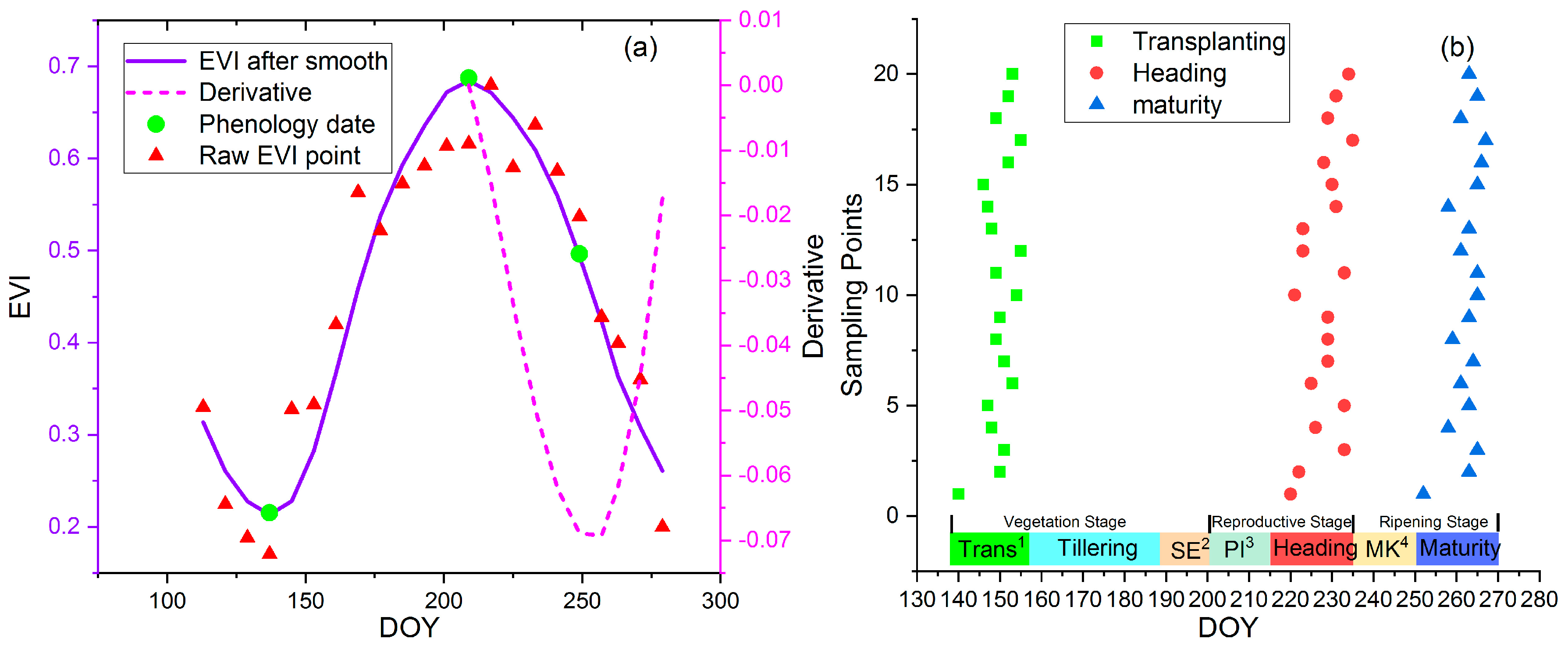
4.1. Remote Sensing Phenology Extraction

Three crucial phenology stages, including transplant, heading, and maturity, were extracted from EVI time series data to optimize the phenology development process in the WOFOST model. The phenological dates are identified with EVI curves according to the rice growth rhythm. Figure 3a shows the EVI time series curve located in one sample point. As can be seen, the EVI curve reaches the lowest value at DOY 140, since the EVI values are affected by the background noise (water and soil) because of the irrigation at the transplanting date. The heading and maturity dates are determined by the date of the EVI curve peak (DOY219) and the date with the largest slope (DOY 252), respectively. Figure 3b illustrates that the three extracted phenological dates at the sample points agree with the local rice phenology calendar obtained from the local meteorological bureau and farmers (Table S3). The spatial distributions of the three rice phenology dates are shown in Figure 4. Due to the hilly topography, the spatial variation in the northeastern Dongting Lake is higher than that in the west. The undulating topography makes the farmland uncontinuous, which increases the difficulty in consentaneous field management. The difference can be observed at the three phenological dates. The outliers of these three phenology images were filtered based on the priori knowledge from the agriculture sector in the study area.

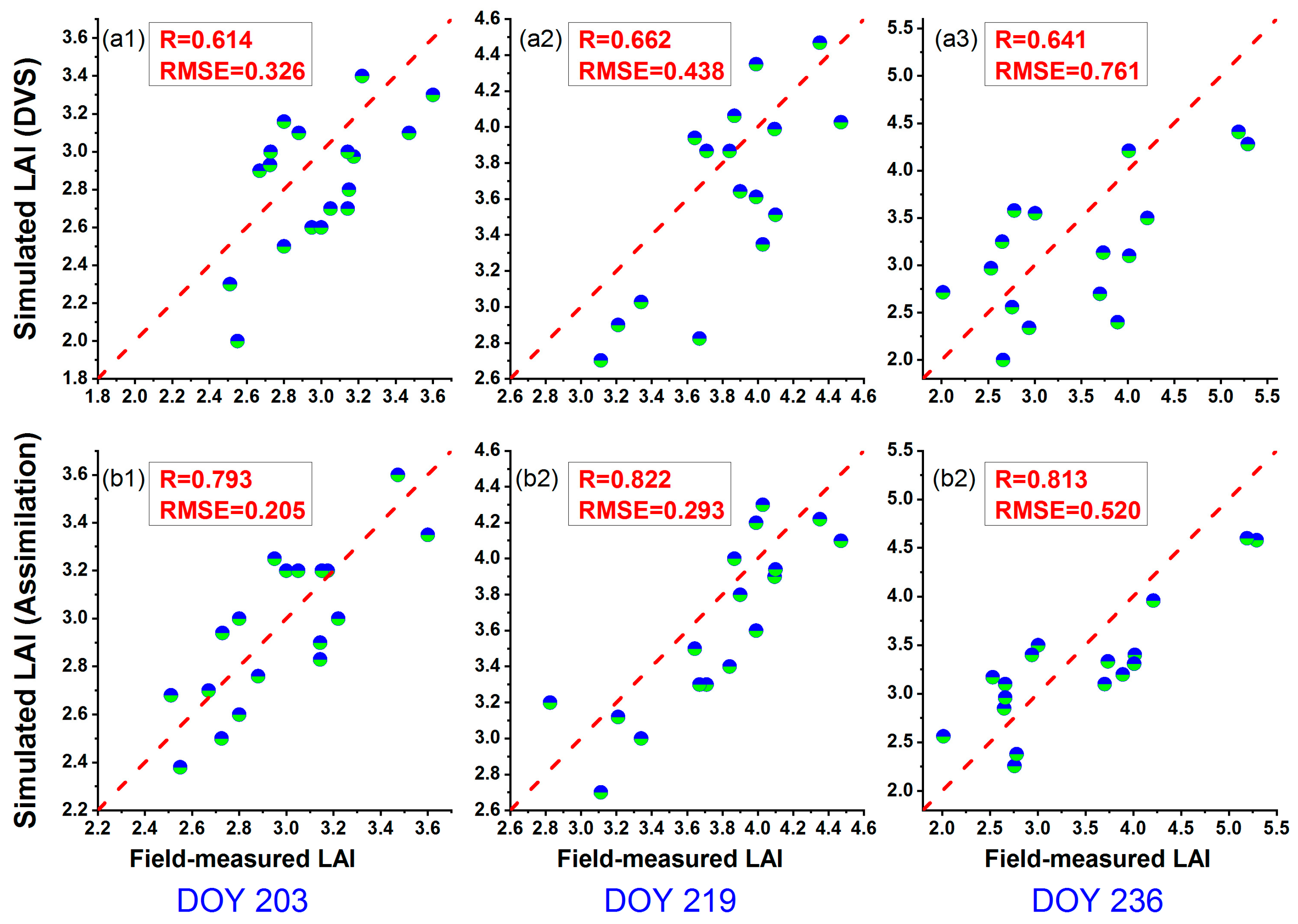
4.2. Rice Growth Simulation with Assimilated Phenological Information

LAI, as the significant biophysical parameter, could provide explicit characteristics of crop growth, thus it was selected to evaluate the performance of the WOFOST model optimized by the proposed method. The correlation coefficient (R) and root mean square error (RMSE) was calculated by the simulated and measured LAI under two conditions: Phenology-based assimilation and without assimilation. As can be seen in Figure 5, the R/ RMSE without assimilation is obviously lower/higher than that with phenology-based assimilation. This result indicates that the assimilation of phenological information effectively improves the performance of the WOFOST model by adjusting IDVS and TD. Meanwhile, the spatial distributions of the WOFOST-simulated LAI with assimilation at different dates are shown in Figure 6. The LAI in the heading period (Figure 6b) is larger than that in the other two periods. The distribution of LAI presents homogeneity and stability in the west of Dongting Lake while LAI in the northeast area shows variability, which is consistent with the distribution of satellite-based phenology (Figure 4). In addition, regarding the scalability assessment of the proposed method, we assimilated phenological information from Landsat 8 EVI time series (30 m) into the WOFOST model. The average LAI are calculated to show the simulation difference between MODIS and Landsat 8 (Figure 7). Although the difference of spatial resolution between MODIS and Landsat 8 is large, the averaged simulated LAI shows little difference in the three experimental areas (less than 0.35). The results indicate that the proposed method can be applied in the farmland with different field sizes, as long as remote sensing time series data with high spatial and temporal resolution are provided.

4.3. Comparison with EVI-Assimilated Rice Growth Simulation

To explore the performance between different assimilation strategy, the EVI time series data was assimilated into a coupled model, which consists of the WOFOST model and PROSAIL model to simulate rice growth, with 8, 10, 12, and 14 images. The structure of the coupled model and the assimilation framework are shown in the Supplementary Materials. The accuracy of LAI simulation and computation time with different assimilation strategies are shown in

Table 1. Accuracy and computation time of rice growth simulation among different assimilation strategies.

Different Strategies	Accuracy (R) a			Computation Time (h)
	DOY203	DOY219	DOY236
Assimilation with Phenology	0.793	0.822	0.813	3.8
Assimilation with EVI (8 images)	0.703	0.714	0.722	8.4
Assimilation with EVI (10 images)	0.741	0.760	0.758	9.2
Assimilation with EVI (12 images)	0.795	0.824	0.810	10.7
Assimilation with EVI (14 images)	0.799	0.818	0.814	12.8
Assimilation with phenology and EVI (12 images)	0.80	0.825	0.816	13.7

Note: ^a The R means the correlation coefficient calculated from simulated and measured LAI.

. As the number of the assimilated image increases, both the computation time and accuracy increase from 0.70–0.72 with eight images to 0.79–0.82 with 12 images. Although the computation time remains growth, the accuracy changes little from 12 images to 14 images, which indicates that assimilating excessive information from remote sensing data increases computational cost without accuracy improvement. Meanwhile, the performance of the proposed assimilation strategy is comparable with that of the strategy with 12 EVI images, while only one-third the computation time is required. Additionally, we assimilated both the 12 EVI time series images and satellite-based phenology into the PROSAIL-WOFOST model for comparison, with an R ranging from 0.80 to 0.82. Although this strategy performed well, the computation cost is the highest. These results indicate that assimilating remote sensing phenology into the WOFOST model is an efficient strategy for rice growth simulation.

5. Discussion

Although previous studies have successfully improved crop models through data assimilation, the strategies relied on biophysical parameters (such as LAI) to optimize the crop physiological development process. Typically, these parameters are obtained with empirical models or a look-up table method, which vary with crop types, time periods, and geophysical conditions. Meanwhile, the assimilation accuracy and efficiency are affected by the selection of satellite data. Therefore, we attempted to establish an assimilation strategy from the perspective of phenology development, which provides an efficient approach for rice growth simulation. In our study, phenological information of rice was extracted from MODIS time series data and assimilated into the WOFOST model to improve the rice growth simulation at the regional scale. The assimilation framework adjusted IDVS and TD by minimizing the difference between simulated and satellite-extracted phenology dates. The results demonstrate that assimilating phenology improves the performance of the WOFOST model, with an R of 0.79–0.82. The result confirms that the proposed strategy could be applied with a different scale. Compared with the assimilation of EVI time series, the accuracy of the proposed strategy is comparable, with less computation time.

The default phenology development in the WOFOST model is not suitable for different crops. For instance, rice grows in farmland after transplantation while this crop model simulates crop growth from emergence. Therefore, the initialization of the phenology development should be adjusted for different crops, especially for rice. Although we optimized the process of the phenology development for rice and adjusted the IDVS in the WOFOST based on remote sensing phenology, the performance of this framework is affected by several factors. Firstly, the rice phenology extraction is influenced by the quality and the resolution (including spatial and temporal resolution) of satellite time series images. In the assessment of the scalability, the effects of thin cloud and shadow were the main error sources, decreasing the accuracy of rice phenological date extraction. Meanwhile, the WOFOST model assumes only three phenology stages during the crop growth season while there are several other phenology stages that affect the crop growth rate. Therefore, the method can be further improved by considering more phenology stages. According to the rice cultivate pattern and growth rhythm, the MODIS EVI products (250 m) were applied in this study to extract rice phenology since the rice fields in the study area are larger than 0.1 km². The spatial resolution of satellite time series data needs to be considered based on the field size when the proposed method is conducted in other regions. For a small rice field, the satellite images with higher spatial and temporal resolution are inevitable for phenology extraction. The fusion and reconstruction of remote sensing imagery have great potential for this challenge.

In addition to uncertainties from phenology extraction, the quantity and quality of measured data impact the simulation performance. Because of the large extent of the study area, the in situ measurement is difficult to acquire, especially for phenology dates. The sample points are sparsely distributed in the study area, which might affect the validation results. Meanwhile, the crop yield, as an important indicator of crop growth, was adopted to validate the simulation accuracy in previous studies [2,13]. Therefore, the crop yield is expected to be obtained as an additional validation indicator in our future work. Additionally, although the WOFOST model was calibrated with multi-source information (Table S1), the spatial distributions of input parameters need to be integrated into the crop model considering the spatial heterogeneity. Quantitative retrieval from satellite data and spatial interpolation will be helpful for the regionalization of the input parameters. Therefore, the localization and regionalization of the model parameters make it possible for accurate crop growth simulation on a regional scale.

6. Conclusions

In this study, we proposed an assimilation strategy from the perspective of phenology development, which effectively improves the rice simulation accuracy of the WOFOST model. The satellite-extracted phenological information was assimilated into the WOFOST model through optimization of IDVS and TD for rice growth simulation. The results show that the performance of the WOFOST model with phenology assimilation is remarkably improved (with R higher than 0.79 and RMSE lower than 0.52 for LAI simulation). The accuracy is comparable with EVI-assimilated strategy (with 12 images) while only one-third the computation time is required. Additionally, the proposed strategy was successfully conducted with different spatial resolution images and a similar simulation result was revealed (difference of simulated LAI_mean less than 0.35 in three experimental areas). This study suggests that assimilating remote sensing phenology into the WOFOST model is an efficient and scalable strategy to improve the performance of the crop model, which provides a novel insight for data assimilation in the field of crop growth simulation.

References

1. Chen, J.S.; Huang, J.X.; Hui, L.; Pei, Z. Rice yield estimation by assimilation remote sensing into crop growth modell. Sci. Sin. 2010, 40, 177–187. [Google Scholar]
2. Huang, J.; Tian, L.; Liang, S.; Ma, H.; Becker-Reshef, I.; Huang, Y.; Su, W.; Zhang, X.; Zhu, D.; Wu, W. Improving winter wheat yield estimation by assimilation of the leaf area index from Landsat TM and MODIS data into the WOFOST model. Agric. For. Meteorol. 2015, 204, 106–121. [Google Scholar] [CrossRef]
3. Mishra, S.K.; Shekh, A.M.; Pandey, V.; Yadav, S.B.; Patel, H.R. Sensitivity analysis of four wheat cultivars to varying photoperiod and temperature at different phenological stages using WOFOST model. J. Agrometeorol. 2015, 17, 74–79. [Google Scholar]
4. Heulen, H.V.; Van Diepen, C. Crop growth models and agro-ecological characterization. In Proceedings of the First Congress of the European Society of Agronomy, Paris, France, 5–7 December 1990; pp. 2–16. [Google Scholar]
5. Bouman, B.A.M.; Keulen, H.V.; Laar, H.H.V.; Rabbinge, R. The ‘School of de Wit’ crop growth simulation models: A pedigree and historical overview. Agric. Syst. 1996, 52, 171–198. [Google Scholar] [CrossRef]
6. Jin, X.; Kumar, L.; Li, Z.; Feng, H.; Xu, X.; Yang, G.; Wang, J. A review of data assimilation of remote sensing and crop models. Eur. J. Agron. 2018, 92, 141–152. [Google Scholar] [CrossRef]
7. Wu, L.; Liu, X.; Wang, P.; Zhou, B.; Liu, M.; Li, X. The assimilation of spectral sensing and the WOFOST model for the dynamic simulation of cadmium accumulation in rice tissues. Int. J. Appl. Earth Observ. Geoinform. 2013, 25, 66–75. [Google Scholar] [CrossRef]
8. Zhao, Y.; Chen, S.; Shen, S. Assimilating remote sensing information with crop model using Ensemble Kalman Filter for improving LAI monitoring and yield estimation. Ecol. Model. 2013, 270, 30–42. [Google Scholar] [CrossRef]
9. Mladen, T.; Rossella, A.; Ljubomir, Z.; Mariethereseabi, S.; Claudio, S.; Pasquale, S. Assessment of AquaCrop, CropSyst, and WOFOST Models in the Simulation of Sunflower Growth under Different Water Regimes. Agron. J. 2014, 101, 509–521. [Google Scholar]
10. Dorigo, W.A.; Zurita-Milla, R.; Wit, A.J.W.D.; Brazile, J.; Singh, R.; Schaepman, M.E. A review on reflective remote sensing and data assimilation techniques for enhanced agroecosystem modeling. Int. J. Appl. Earth Observ. Geoinform. 2007, 9, 165–193. [Google Scholar] [CrossRef]
11. Liang, S.; Qin, J. Data Assimilation Methods for Land Surface Variable Estimation; Springer: Amsterdam, The Netherlands, 2008; pp. 313–339. [Google Scholar]
12. Ahmadalipour, A.; Moradkhani, H.; Yan, H.; Zarekarizi, M. Remote sensing of drought: Vegetation, soil moisture, and data assimilation. In Remote Sensing of Hydrological Extremes; Springer: Berlin, Germany, 2017; pp. 121–149. [Google Scholar]
13. Chen, Y.; Zhang, Z.; Tao, F. Improving regional winter wheat yield estimation through assimilation of phenology and leaf area index from remote sensing data. Eur. J. Agron. 2018, 101, 163–173. [Google Scholar] [CrossRef]
14. Maas, S.J. Use of remotely-sensed information in agricultural crop growth models. Ecol. Model. 1988, 41, 247–268. [Google Scholar] [CrossRef]
15. Moulin, S.; Bondeau, A.; Delecolle, R. Combining agricultural crop models and satellite observations: From field to regional scales. Int. J. Remote Sens. 1998, 19, 1021–1036. [Google Scholar] [CrossRef]
16. Huang, J.; Ma, H.; Su, W.; Zhang, X.; Huang, Y.; Fan, J.; Wu, W. Jointly assimilating MODIS LAI and ET products into the SWAP model for winter wheat yield estimation. IEEE J. Sel. Top. Appl. Earth Obs. Remote Sens. 2015, 8, 4060–4071. [Google Scholar] [CrossRef]
17. Huang, J.; Sedano, F.; Huang, Y.; Ma, H.; Li, X.; Liang, S.; Tian, L.; Zhang, X.; Fan, J.; Wu, W. Assimilating a synthetic Kalman filter leaf area index series into the WOFOST model to improve regional winter wheat yield estimation. Agric. For. Meteorol. 2016, 216, 188–202. [Google Scholar] [CrossRef]
18. Huang, J.; Ma, H.; Sedano, F.; Lewis, P.; Liang, S.; Wu, Q.; Su, W.; Zhang, X.; Zhu, D. Evaluation of regional estimates of winter wheat yield by assimilating three remotely sensed reflectance datasets into the coupled WOFOST–PROSAIL model. Eur. J. Agron. 2019, 102, 1–13. [Google Scholar] [CrossRef]
19. Bouman, B.A.M. Linking physical remote sensing models with crop growth simulation models, applied for sugar beet. Int. J. Remote Sens. 1992, 13, 2565–2581. [Google Scholar] [CrossRef]
20. Weiss, M.; Troufleau, D.; Baret, F.; Chauki, H.; Prévot, L.; Olioso, A.; Bruguier, N.; Brisson, N. Coupling canopy functioning and radiative transfer models for remote sensing data assimilation. Agric. For. Meteorol. 2001, 108, 113–128. [Google Scholar] [CrossRef]
21. Li, H.; Chen, Z.; Liu, G.; Jiang, Z.; Huang, C. Improving Winter Wheat Yield Estimation from the CERES-Wheat Model to Assimilate Leaf Area Index with Different Assimilation Methods and Spatio-Temporal Scales. Remote Sens. 2017, 9, 190. [Google Scholar] [CrossRef]
22. Jin, M.; Liu, X.; Wu, L.; Liu, M. An improved assimilation method with stress factors incorporated in the WOFOST model for the efficient assessment of heavy metal stress levels in rice. Int. J. Appl. Earth Observ. Geoinform. 2015, 41, 118–129. [Google Scholar] [CrossRef]
23. Cheng, Z.; Meng, J.; Wang, Y. Improving Spring Maize Yield Estimation at Field Scale by Assimilating Time-Series HJ-1 CCD Data into the WOFOST Model Using a New Method with Fast Algorithms. Remote Sens. 2016, 8, 303. [Google Scholar] [CrossRef]
24. Huang, X.; Huang, G.; Yu, C.; Ni, S.; Yu, L. A multiple crop model ensemble for improving broad-scale yield prediction using Bayesian model averaging. Field Crops Res. 2017, 211, 114–124. [Google Scholar] [CrossRef]
25. Liu, F.; Liu, X.; Ding, C.; Wu, L. The dynamic simulation of rice growth parameters under cadmium stress with the assimilation of multi-period spectral indices and crop model. Field Crops Res. 2015, 183, 225–234. [Google Scholar] [CrossRef]
26. Wu, L.; Liu, X.; Wang, C.; Qin, Q.; Zheng, X.; Sun, Y. Temporal scale optimization for assimilation of spectral information and crop growth model. Trans. Chin. Soc. Agric. Eng. 2015, 142–148. [Google Scholar]
27. Sakamoto, T.; Yokozawa, M.; Toritani, H.; Shibayama, M.; Ishitsuka, N.; Ohno, H. A crop phenology detection method using time-series MODIS data. Remote Sens. Environ. 2005, 96, 366–374. [Google Scholar] [CrossRef]
28. Zheng, H.; Cheng, T.; Yao, X.; Deng, X.; Tian, Y.; Cao, W.; Zhu, Y. Detection of rice phenology through time series analysis of ground-based spectral index data. Field Crops Res. 2016, 198, 131–139. [Google Scholar] [CrossRef]
29. Dong, J.; Xiao, X.; Kou, W.; Qin, Y.; Zhang, G.; Li, L.; Jin, C.; Zhou, Y.; Wang, J.; Biradar, C. Tracking the dynamics of paddy rice planting area in 1986–2010 through time series Landsat images and phenology-based algorithms. Remote Sens. Environ. 2015, 160, 99–113. [Google Scholar] [CrossRef] [Green Version]
30. Boogaard, H.L.; van Diepen, C.A.; Rutter, R.P.; Cabrera, J.M.C.A.; Laar, H.H. User’s Guide for the WOFOST 7.1 Crop Growth Simulation Model and WOFOST Control Center 1.5; Winand Staring Centre for Integrated Land, Soil and Water Research: Wageningen, The Netherlands, 1998. [Google Scholar]
31. Onojeghuo, A.O.; Blackburn, G.A.; Wang, Q.; Atkinson, P.M.; Kindred, D.; Miao, Y. Rice crop phenology mapping at high spatial and temporal resolution using downscaled MODIS time-series. GISci. Remote Sens. 2018, 55, 659–677. [Google Scholar] [CrossRef]
32. Peng, D.; Huete, A.R.; Huang, J.; Wang, F.; Sun, H. Detection and estimation of mixed paddy rice cropping patterns with MODIS data. Int. J. Appl. Earth Observ. Geoinform. 2011, 13, 13–23. [Google Scholar] [CrossRef]
33. Liu, Z.; Hu, Q.; Tan, J.; Zou, J. Regional scale mapping of fractional rice cropping change using a phenology-based temporal mixture analysis. Int. J. Remote Sens. 2018, 1–14. [Google Scholar] [CrossRef]
34. Yuan, Y.; Zhang, C.; Zeng, G.; Liang, J.; Guo, S.; Huang, L.; Wu, H.; Hua, S. Quantitative assessment of the contribution of climate variability and human activity to streamflow alteration in Dongting Lake, China. Hydrol. Process. 2016, 30, 1929–1939. [Google Scholar] [CrossRef]
35. Qi, X.; Fu, Y.; Wang, R.Y.; Ng, C.N.; Dang, H.; He, Y. Improving the sustainability of agricultural land use: An integrated framework for the conflict between food security and environmental deterioration. Appl. Geogr. 2018, 90, 214–223. [Google Scholar] [CrossRef]
36. Lu, R. Analytical Methods of Soil and Agricultural Chemistry; China Agricultural Science and Technology Press: Beijing, China, 1999; pp. 107–240. [Google Scholar]
37. Didan, K.; Munoz, A.B.; Solano, R.; Huete, A. MODIS Vegetation Index User’s Guide (MOD13 Series); Vegetation Index and Phenology Lab., University of Arizona: Tucson, AZ, USA, 2015. [Google Scholar]
38. Diepen, C.A.; Wolf, J.; Keulen, H.; Rappoldt, C. WOFOST: A simulation model of crop production. Soil Use Manag. 2010, 5, 16–24. [Google Scholar] [CrossRef]
39. Wardlow, B.D.; Egbert, S.L. A comparison of MODIS 250-m EVI and NDVI data for crop mapping: A case study for southwest Kansas. Int. J. Remote Sens. 2010, 31, 805–830. [Google Scholar] [CrossRef]
40. Fan, L.; Luo, Z.Z. Rice yield estimation based on MOSIS-NDVI: Case study of Chongqing Three Gorges warehouse district. Southwest China J. Agric. Sci. 2009, 1416–1419. [Google Scholar]
41. Chen, P.Y.; Fedosejevs, G.; Tiscareño-López, M.; Arnold, J.G. Assessment of MODIS-EVI, MODIS-NDVI and VEGETATION-NDVI Composite Data Using Agricultural Measurements: An Example at Corn Fields in Western Mexico. Environ. Monit. Assess. 2006, 119, 69–82. [Google Scholar] [CrossRef] [PubMed]
42. Wang, Z.; Liu, C.; Alfredo, H. From AVHRR-NDVI to MODIS-EVI: Advances in vegetation index research. Acta Ecol. Sin. 2003, 23, 979–987. [Google Scholar]
43. Jönsson, P.; Eklundh, L. TIMESAT—A program for analyzing time-series of satellite sensor data. Comput. Geosci. 2004, 30, 833–845. [Google Scholar] [CrossRef]
44. Jonsson, P.; Eklundh, L. Seasonality extraction by function fitting to time-series of satellite sensor data. IEEE Trans. Geosci. Remote Sens. 2002, 40, 1824–1832. [Google Scholar] [CrossRef]
45. Li, S.H.; Xiao, J.T.; Ni, P.; Zhang, J.; Wang, H.S.; Wang, J.X. Monitoring paddy rice phenology using time series MODIS data over Jiangxi Province, China. Int. J. Agric. Biol. Eng. 2014, 7, 28–36. [Google Scholar]
46. You, X.; Meng, J.; Zhang, M.; Dong, T. Remote Sensing Based Detection of Crop Phenology for Agricultural Zones in China Using a New Threshold Method. Remote Sens. 2013, 5, 3190–3211. [Google Scholar] [CrossRef] [Green Version]
47. Yu, F.; Price, K.P.; Ellis, J.; Shi, P. Response of seasonal vegetation development to climatic variations in eastern central Asia. Remote Sens. Environ. 2003, 87, 42–54. [Google Scholar] [CrossRef]
Figure 1. Overview of the study area. (a) Location of the study area and the land cover types in 2015 provided by the GFSAD30AUNZCNMOCE product. (b) The distribution of rice farmland and three experimental areas in the study area. (c) The size of a typical rice field from Google Earth (larger than 0.1 km2). (d) Illustration of the sampling approach.
Remotesensing 11 00268 g001
Figure 2. Flowchart of rice growth simulation optimization with satellite-based phenology and the WOFOST model.
Remotesensing 11 00268 g002
Figure 3. (a) Phenology extraction from EVI timeseries data at one sample point; (b) extracted phenological dates at sample points together with rice phenology calendar (Note: 1 transplanting date, 2 Stem elongation, 3 Panicle initiation, 4 Milking).
Remotesensing 11 00268 g003
Figure 4. Spatial distribution of three phenology time in the study area at the (a) transplant date; (b) heading date; (c) maturity date.
Remotesensing 11 00268 g004
Figure 5. The performance of rice growth simulation under two conditions. (a1a3): no data assimilation; (b1b3): phenology-based assimilation.
Remotesensing 11 00268 g005
Figure 6. Spatial-temporal distribution of WOFOST-simulated LAI.
Remotesensing 11 00268 g006
Figure 7. The difference of simulated mean LAI between MODIS data and Landsat 8 data at different time in three experimental areas.
Remotesensing 11 00268 g007