Estimating the Height and Basal Area at Individual Tree and Plot Levels in Canadian Subarctic Lichen Woodlands Using Stereo WorldView-3 Images

Geography Department, Université du Québec à Montréal, Montréal, QC H3C 3P8, Canada
*
Author to whom correspondence should be addressed.
Remote Sens. 2019, 11(3), 248; https://doi.org/10.3390/rs11030248
Submission received: 12 December 2018
/
Revised: 21 January 2019
/
Accepted: 22 January 2019
/
Published: 26 January 2019
(This article belongs to the Special Issue Remote sensing based Forest Inventories from Landscape to Global Scale)
Abstract
:Lichen woodlands (LW) are sparse forests that cover extensive areas in remote subarctic regions where warming due to climate change is fastest. They are difficult to study in situ or with airborne remote sensing due to their remoteness. We have tested a method for measuring individual tree heights and predicting basal area at tree and plot levels using WorldView-3 stereo images. Manual stereo measurements of tree heights were performed on short trees (2–12 m) of a LW region of Canada with a residual standard error of ≈0.9 m compared to accurate field or UAV height data. The number of detected trees significantly underestimated field counts, especially in peatlands in which the visual contrast between trees and ground cover was low. The heights measured from the WorldView-3 images were used to predict the basal area at individual tree level and summed up at plot level. In the best conditions (high contrast between trees and ground cover), the relationship to field basal area had a R2 of 0.79. Accurate estimates of above ground biomass should therefore also be possible. This method could be used to calibrate an extensive remote sensing approach without in-situ measurements, e.g., by linking precise structural data to ICESAT-2 footprints.
1. Introduction
Lichen woodlands (LW), and more generally northern open canopy forests, cover extensive areas in the circumpolar subarctic regions. The naming (e.g., “taiga”) and definition (e.g., latitude range) of these forests vary [1]. Some authors [2,3] distinguished three zones from south to north (approximately 50° to 70° north) which they called respectively closed-canopy boreal forests, open canopy woodlands and forest-tundra. Others have more recently defined LW as an ecotone stretching between closed canopy boreal forests and tundra [4,5,6], i.e., a boreal-arctic transition. We will here adopt the latter definition and consider the LW as having a geographical distribution in Canada and Alaska as presented in the map proposed in Reference [4] (Figure 1). According to this definition, subarctic forest cover approximately 2 × 10⁶ km2 in Canada alone. They are characterized by short growing seasons, temperatures varying from 20 °C in summer to −50 °C in winter, and a discontinuous permafrost. Their plant diversity is poor, especially in the case of treed vegetation. In Canada, black spruce (Picea mariana [Mill.] BSP.), jack pine (Pinus banksiana [Lamb.]) and eastern larch (Larix laricina [Du Roy Koch.]) constitute the large majority of LW trees, with the former species being largely predominant. LW are characterized by short and open canopies, and a forest floor mostly covered by lichens (see Figure 2). Although their above ground biomass density (t ha−1, thereafter termed “biomass”) is currently low, a lengthening of the growing season, CO2 fertilization, and the consequent rise in productivity of LW could have a significant global impact on carbon sequestration due to the extensiveness of these woodlands [7,8]. According to Ouranos [9], the length of the growing season in subarctic regions could increase by 20 days by 2050, while the average annual temperature could rise by 3 °C during the same period. This could cause a densification of northern woodlands [10] and an increase of tree height and biomass. Other factors, such as the forest fire regime, could nevertheless cause a migration of LW towards the south [5]. Precisely describing the current state of the boreal-tundra ecotone LW and following their evolution in the coming decades, is, therefore, becoming ever more important. In particular, methods allowing the accurate estimation of the factors that determine the above ground biomass density, such as tree height, basal area (BA) and stem density (stems ha−1) should be deployed over LW to better describe their structure and carbon contents. Compared to the continuous boreal forests, subarctic forests have, however, been much less studied [11]. This can be explained by their low to null commercial interest and their remoteness [12]. The road density in these areas is extremely low, and the airports are very sparse. This makes field work or airborne surveys complicated and extremely expensive, at least in the far north regions of Canada or Russia, and with that, much less intensive than in the southern boreal forest.
The key measurements for assessing tree biomass are the height and geolocation of individual trees because diameter at breast height can be predicted from height (e.g., Reference [13]), biomass from height and DBH, and stem density can be obtained by simply tallying the number of trees located within a given area. Apart from field measurements, individual tree heights can be well estimated using photogrammetric methods [14]. In sparse forests, heights can be obtained from single aerial photographs (in monoscopic mode) using the radial displacement of trees viewed obliquely, or by the length of their shadows [15]. More often, the height is calculated based on parallax differences on stereoscopic pairs of photographs [14,15], a method often referred to as “spatial intersection” of the conjugate rays. In the former case, both the top and the base of the tree (or its shadow) must be visible, which is not always the case, even in sparse woodlands. In the latter case, the top of the targeted tree must be seen in both photographs to enable spatial intersection, yielding the XYZ position of the tree top. By measuring the ground elevation near the tree in the same way, or by extracting it from an airborne laser scanning (ALS) digital terrain model [16], the height of the tree can be calculated. The accuracy of the elevation measurement of the tree top depends on the shape of the tree and the spatial resolution of the images. For trees having a tapering crown, underestimation is expected because the tip of the tree often cannot be resolved. For example, Spurr [15] reported an underestimation ranging from 0.6 m at a photographic scale of 1:10,000, to 1.5 m at a scale of 1:20,000 for elongated trees, for analog aerial photographs. For the same scales but for broad crowns, the underestimations were respectively 0.0 m and 0.3 m. All the above methods have so far been exclusively applied to aerial imagery. In theory, such measurements could also be made on high-resolution satellite images. While high-resolution airborne photographic surveys are, as previously mentioned, rather complicated and costly in remote subarctic regions, earth observation from space does not entail logistical difficulties. To the best of our knowledge, however, measurements of individual tree height from space have never been accomplished.
Since 1999, with the launch of the IKONOS sensor [17], earth observation from space can supply images having a ground sampling distance of 1 m or less. These are often referred to as high-resolution spaceborne images (HRSI), although the meaning of this acronym may vary. Few studies have attempted to characterize the structure of northern open canopy forests using HRSI. Leboeuf et al. [18,19] proposed a method for mapping biomass, basal area and wood volume based on the retrieval of the proportion of shadows from QuickBird images (0.61 m ground sampling distance), followed by statistical modelling, yielding relative root mean square errors (RMSE) of 17–32%. Although the shadow length, as determined by tree height, certainly influenced the results, the method was not based on measuring it specifically. Only the overall proportion of shadows per plot was statistically linked to biomass. A related approach, but applied at the individual tree level, consisted in using shadow area to predict stem volume, achieving an R2 of 0.61 [20]. However, because shadow-based methods are influenced by the sun elevation at the time of image acquisition, the regression models used to predict biomass are only valid for the images for which they were calibrated, thus hindering generalization. Other studies proceeded by creating a digital surface model (DSM) using stereo image matching, and then by subtracting ground heights provided by either ALS (e.g., Reference [21]), or by a digital terrain model (DTM) extracted from the photogrammetric point cloud itself. Montesano et al. [12] combined stereo WorldView-1 images (0.46 m ground sampling distance) and ICESat-GLAS waveforms [22] to estimate the height of trees in northern Siberia with a RMSE varying from 0.85 to 1.37 m. In this case, the Worldview-1 imagery was used only to assess the ground-level elevations, not the top of the trees. Later for the same region, Montesano et al. [6] used WorldView-1 and -2 stereo-images to reconstruct both the ground and vegetation elevations using the image matching algorithm of the AMES stereo pipeline of NASA [23]. By comparing results obtained from imagery acquired with sun elevations varying from 7° to 43°, they found that the highest accuracy for the DTM reconstruction was achieved in high sun elevation conditions (RMSE < 0.68 m), whereas a low sun elevation was preferable for characterizing vegetation heights. Meddens et al. [24] used the 5-m resolution ArcticDEM [25] elevation product to estimate canopy height in Alaska. The vegetated ArcticDEM pixels identified using multispectral imagery were replaced by values interpolated from non-vegetated pixels. By subtracting the original ArcticDEM with the modified version, an approximate canopy height model (CHM) was created. Forest heights were then predicted with a RMSE generally between 2–3 m by combining this CHM with several other monoscopic predictors derived from WorldView-2 imagery. The calibration of the regression model, however, required several thousand calibration points extracted from ALS data. Several other studies concerned the creation of DSMs over forest canopied using stereo HRSI, albeit not in subarctic woodlands (e.g., References [25,26,27,28,29]).
Considering the narrowness of the crowns of subarctic trees, even a ground sampling distance of 0.5–1.0 m is probably insufficient to reconstruct the height of narrow-crown black spruces. Digital Globe launched the Worlview-3 (WV3) satellite in 2014 [30], followed by WorldView-4 (WV4) in 2016. Both provide images with a nominal ground sampling distance of 0.31 m at nadir in panchromatic mode, as well as stereo capacity and several narrower spectral bands at a coarser resolution. Starting in 2020, the Pléiades NEO constellation of four satellites with tri-stereo capacity should start producing images at a resolution of 30 cm [31]. For disambiguation, we will thereafter term the latter class of imaging sensors (pixel size < 0.50 m) “very high resolution spaceborne imaging” (VHRSI). Images from WV3 or WV4 are designed to have a high photogrammetric quality and can be used to generate DSM using automated image matching techniques. Accuracy assessments relative to these sensors are, however, still rare, and none of the existing studies concerned subarctic forests. Aguilar and et al. [32] used WV3 stereo pairs to generate DSMs of different surface types. Compared to a lidar dataset, a RMSE of 0.26 m (compared to ALS) was observed over bare ground surfaces for DSMs generated using the RPC stereo processor matching algorithm [33]. This confirms the high photogrammetric quality of WV3 images and demonstrated the high performance of the matching algorithm for the simplest type of surface. Goldbergs et al. [34], however, showed that commercial stereo image matching software (PCI Geomatica, Canada, and Photomod from Racurs, Russia) designed to work with spaceborne images acquired with pushbroom sensors (here GeoEye and WorldView-1), failed to properly reconstruct the vertical structure of open canopies. Although this study was conducted in an Australian savannah, it illustrates the image matching challenges over sparse woodlands.
In general, the quality of photogrammetric data extracted from stereo-pairs of VHRSI with regard to detailed forest structure characterization depends on certain fundamental factors that are independent of the image matching method. First, the tree tops must be visible (non-occluded) in the two images forming a stereo-pair, and must be discernable from other trees, or from other objects such as the underlying ground cover [14]. Therefore, occlusions, or lack of contrast and resolution, impedes on establishing the stereo correspondence. Contrast itself depends on the radiometric properties of the objects and on the radiometric resolution of the sensor. Second, the photogrammetric quality of the sensor (i.e., distortions-free optics, well calibrated internal orientation, etc.), and the capacity of the platform to achieve a viewing geometry (convergence, bisector and asymmetry angles of the conjugate rays, see References [35,36]) that provides good conditions for spatial intersection affect the accuracy of the height measurements. We assert that it is important to assess the impact of the above factors separately from the evaluation of the quality of a derived DSM, because the latter is also altered by the image matching uncertainty.
Moreover, although ALS can provide individual heights even for small trees of northern regions when the laser point density is fairly high [37], it is logistically difficult to perform ALS surveys due to the scarcity of airports. What is more, using a lower point density would logically result in many narrow crowns of black spruces being missed as some would lie between scan lines. A few airborne lidar acquisition attempts were made in northern Canada, for example by Margolis et al. [38] using PALS, a laser profiler mounted on a small aircraft. To the best of our knowledge, the largest ALS survey of northern forests of Canada was carried out by Hopkinson et al. [39]. They used an Optech ALTM3100 system to acquire strips of data with a swath width of 640 m, over a total length of 24,000 km between the latitudes of 43°N and 65°N, and with a point density of at least 1 point/m2. This was a rather unique endeavour that is unlikely to the repeated regularly.
While airborne surveys are difficult, lidar Earth observation spaceborne platforms provide only partial solutions. LW regions in Canada indeed fall in great part within a latitude range [5] that is not covered by important programs such as data acquisition with the GEDI spaceborne mission [40], that does not cover regions north of 51.6°N, nor by the ArcticDEM program [25], that only covers regions above 60°N. Only the ICESat-2 mission [41], launched on September 15, 2018, will provide sparse 3D point clouds for LW. It will, however, do so in a spatially discontinuous manner, and with a spatial resolution (17 m diameter footprints) insufficient to precisely characterize the structure of subarctic forests.
Our main objective was therefore to assess the accuracy of manual individual tree height measurements performed by spatial intersection of conjugate rays on stereo WorldView-3 images of an open-crown Canadian subarctic forest. In addition, we wanted to verify that the plot-level basal area (in m2 ha−1), as a surrogate to biomass, can be predicted from the tree heights. This implies that most trees would have to be detected on both images of the stereo-pair. For this reason, our aim was also to assess the accuracy of density estimates of detectable trees (in stems ha−1). The level of tree detectability (non-occluded and discernable) was assessed for different ground covers to verify the effect of contrast between trees and their background. We performed the stereo measurements manually to ensure that the results depended only on the inherent information content of the imagery rather than on the quality of an image matching algorithm. Indeed, what cannot be retrieved manually because of lack of contrast or occlusions would neither appear in photogrammetric point clouds derived automatically. However, detectable individual trees may be badly reconstructed or entirely missed by automated stereo reconstruction.
The methods presented in this study were developed to potentially serve two purposes. The first is to allow building a better characterization of the structure variability of LW by facilitating localized sampling in remote areas using remote sensing means only, thus avoiding the costs and logistical problems of in-situ measurements. The second was to enable researchers to create “virtual plots” anywhere in LW, in sizes and shapes adapted to the calibration procedures of other remote sensing data, such as ICESAT-2, again without field campaigns.
2. Materials and Methods
2.1. Study Area
Field data and imagery were acquired within a 102 km2 area (centered on 78.7°W, 53.7°N) located near the La Grande River, in the Chisasibi municipality of the province of Quebec, Canada (Figure 3). The study area lies within the LW bioclimatic domain [5] (Québec, 2016). Its subarctic climate is characterized by average temperatures of −3 °C and average annual precipitations of 684 mm. The growing season lasts approximately 130 days, with roughly 700-degree days of growth (according to maps published in Reference [42]). Topography is nearly flat (elevations vary from 18 to 68 m above sea level), and soils are thin, sandy and well drained in most areas, except in peatlands, where the organic layer can reach important depths.
The most common vegetation formations are sparse woodlands growing on sandy soils covered by cladonia species (e.g., Cladonia stellaris [Opiz. Pouzar & Vĕzda]), i.e., white fruticose lichens approximately 10 cm in height. At least 95% of trees are black spruces, which are accompanied by a few larches and jack pines. The trees sometime reach 12 m in height, but most are less than 10 m high, notably because of their very slow growth (5–11 cm y−1). Their crowns are very narrow and often terminated by a thick and sometimes roundish volume of shoots (Figure 2). Part of the territory is occupied by peatlands sparsely covered by similar trees, but having a different ground cover, which is composed mostly of mosses, herbaceous species and Labrador tea (Rhododendron groenlandicum [(Oeder) Kron & Judd]). Some denser patches of forests can also be found, but these occupy only a small fraction of the study area.
2.2. Field Data
Tree measurements and unmanned aerial vehicle (UAV) flybys were carried out in the field from 24 July to 11 August 2017 in 14 well-distributed circular field plots (Figure 3). The plots had radii from 9.77 m to 12.62 m (with plot areas respectively from 300 m2 to 500 m2) depending on the local density of trees. We categorized the plots’ ground cover types as lichen, rocky or peatland. Two different measurement protocols were used. In “standard” plots, the DBH and species of all trees having a height of 2 m or more were recorded. In addition, the height and XY position of five trees representative of the plot’s height distribution were measured. In “intensive” plots, the DBH, species, height and XY location of all trees of 2 m or more were recorded. In addition, five trees per intensive plot (total of 30 trees) were felled and their height was precisely measured with a distance tape after felling. Table 1 summarizes the plot information. The density may appear high therein. This is because the very low size threshold (height < 2 m) for including trees created large totals per plot, with many trees having a DBH of only 2 cm. It is to be contrasted to the majority of forest studies, which use a much larger threshold (e.g., DBH ≥ 9 cm) resulting in lower densities.
DBH larger than 4 cm were measured to the nearest mm using a DBH tape. Smaller ones were measured with a fixed-increment caliper, with increments of 1, 2 and 4 cm. The heights were measured with a Sokkia telescopic height pole for trees not exceeding 8 m, and with a Vertex III instrument (Haglöf, Långsele, Sweden) for taller ones. For pole measurements, one operator standing next to the tree deployed the telescopic segments and read the height on the display while another ascertained from a distance that the tip of the pole was level with the tree extremity. In the case of Vertex measurements, the apex of all trees could be precisely seen and was viewed at an angle of approximately 45°. Using the height data from felled trees, the bias of the non-destructive field height measurements (pole or Vertex) was assessed and corrected. Moreover, the position of the trees was measured relative to the plot center by using the Vertex in distance mode. Three reference points were precisely placed at 2 m horizontally from the plot center in respectively the N, SE and SW directions. For each tree, a distance measurement was performed from each reference point. For this procedure, the Vertex was mounted on a supporting pole equipped with a bubble level to ensure its verticality over each reference point during the measurements. The XY positions of trees relative to the plot center were then determined using trilateration. Before initial measurements, and at approximately 30-min intervals, the Vertex instrument was recalibrated to account for eventual changes in air temperature and humidity that might affect the accuracy of its distance measurements, which are based on ultrasound pulses. The relative tree positions were later translated to the absolute plot center location obtained by GNSS positioning (details follow).
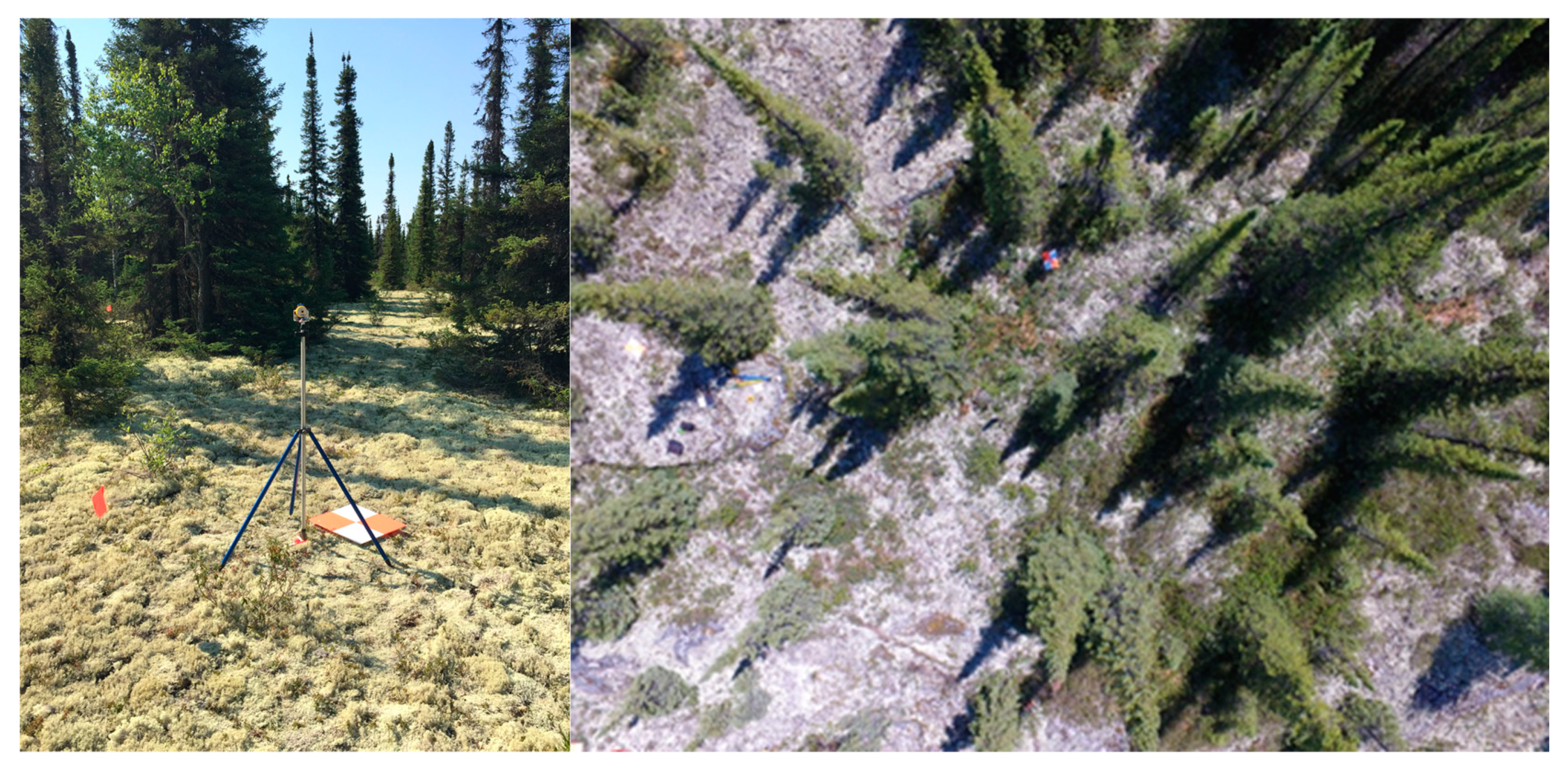
For all plots, a small UAV (DJI Phantom 3 4k, equipped with a Sony Exmor camera) was used to take still images from an altitude of approximately 20 m above ground. The camera had a focal length of 3.6 mm and a focal plane size of 6.317 mm by 4.738 mm, with 1.57 µm pixels. Viewpoints roughly laid out as a regular lattice provided an image overlap of 85–90% in both directions. The ground sampling distance of the images was approximately 1 cm. Prior to the UAV surveys, four targets (panels with a center mark, see Figure 2) visible from the air were laid out in the plot directly on the ground. One was placed at the exact plot center and three others at the periphery, separated by 120 degrees. These targets, serving as ground control points (GCPs), were surveyed with a SX-Blue 2 GNSS receiver (GPS and GLONASS) from Geneq Inc. (Montreal, Canada). In addition, eight ground elevations were measured in each plot with the GNSS receiver using the above procedure. Two measurements were done in each cardinal direction between the center (already measured) and the periphery, resulting in a cross pattern.
Finally, seven well distributed GCPs for georeferencing the WorldView-3 image pair (Figure 3) were geopositioned using the same GNSS procedure. The GCPs corresponded to minute and fixed objects visible on the satellite images, e.g., a white stone emerging from a darker background, the corner of a concrete block, etc. Terrestrial photos were taken at each location during the GNSS positioning to ensure that the pinpointing of the GCP pixels on the images corresponded to the exact field position of the GNSS receiver.
For all acquired positions, the GNSS antenna was mounted on top of a 2-m support pole held vertically on the measured point. Antenna height above ground was subtracted from the Z measurements. Positions were corrected in real-time using the Wide Area Augmentation System. GNSS signals were integrated for 1 min at each station and the final geolocation was obtained by computing the average of the 60 positions. During the collection of all GCPs (for plot positioning, UAV image orientation and WV3 image georeferencing), the GNSS point dilution of precision (PDOP) was generally 1.3 or 1.4.
2.3. Remote Sensing Imagery
A Digital Globe WorldView-3 stereo pair was acquired on 7 July 2018 with a convergence angle of approximately 37°. No clouds or haze were present at the acquisition time. Each of the two images was composed of a panchromatic band at 0.31 m nominal ground sampling distance at the nadir and eight spectral bands at 1.24 m resolution [43]. The images were obtained in orthoready 16-bit format (2A) with their rational polynomial coefficients (RPC). The detailed image characteristics and acquisition parameters appear in Table 2.
2.4. Image Georeferencing
To create the precisely oriented WV3 stereo-model, 30 tie points between the images were manually picked, and the image pair was tied to the 7 GCPs. This resulted in an adjustment of the initial RPC values. This operation was performed using Summit Evolution Professionnal v 7.4 (DAT/EM Systems International, Anchorage, AK, USA). The UAV images were first aero-triangulated using the approximate principal point positions given by the UAV’s GPS data and tie points were automatically generated. For each plot, the aero-triangulated block was then tied to the four geolocated ground targets visible in the images. The above orientation procedures of the UAV images were performed using Pix4Dmapper v.4.1.24 (Pix4D, Lausanne, Switzerland).
2.5. Tree Height Measurements and Stem Counts from the WV3 Images
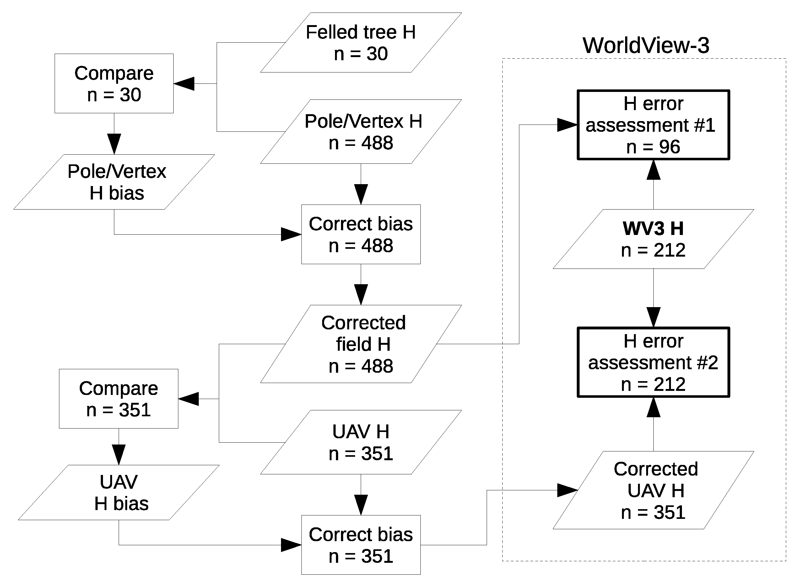
The method for assessing the accuracy of tree height (H) measurements from WV3 stereo images aimed to compare these to the best available reference height data and for the largest number of trees. Because the measurements of heights in the field are time consuming, they were not performed on all trees within the standard plots. For these, we have instead used bias-corrected tree heights extracted from 3D point clouds derived from the UAV images using dense stereo matching. Height measurements from low altitude UAV images have been shown to be accurate [44]. These UAV point clouds also helped in establishing the correspondence between the field and WV3 heights. Moreover, even heights measured in the field using a height pole or the Vertex contained small errors. To avoid any bias in the assessment of the error of WV3 based on reference tree height measurements, we have:
- Estimated the bias between the pole/Vertex heights and the true height measured on the corresponding felled trees (n = 30), and then corrected all the non-destructive height measurements accordingly;
- estimated the bias between the bias-corrected field heights and the corresponding heights extracted from the UAV 3D point clouds, and then corrected all the UAV heights accordingly.
To measure heights from the UAV data, image matching was performed using Pix4dMapper to create a dense 3D point cloud. The ground points were then identified using the lasground function of LAStools (rapidLasso GmbH) with a value of 1.75 for the step parameter. A DTM was created by interpolating these ground points using the LAS dataset to Raster function of ESRI’s ArcMap v. 10.5, taking the average of values falling in each cell. The highest point on the tree apex was identified manually by inspecting the raster values, and the local DTM elevation was subtracted from it to estimate tree height. The bias of this these measurements was assessed by computing the average difference between the bias-corrected field tree heights and the corresponding UAV tree heights (n = 351). This bias was then removed from the UAV heights.
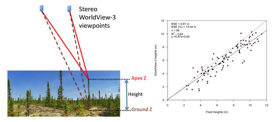
The height of individual trees was measured manually using stereo viewing of pansharpened color WV3 image with LCD shutter glasses within Summit Evolution v. 7.4 (DAT/EM Systems International, Anchorage, AK, USA), a software application for capturing 3D information from stereo data. A color composite of the green, red and infrared channels was sharpened with the panchromatic band and contrast-stretched to improve the visual discernibility of trees compared to the black and white panchromatic images. For all trees for which the apex was clearly visible in both images of the stereo pair, the interpreter digitized the 3D position of the apex and that of the nearest visible ground point. This point was in most cases very near the tree (e.g., 1 m), but in denser plots, it sometimes had to be selected some distance away from the tree (e.g., 3–4 m). Because of local topographical variations, greater distances from the tree increase the risk of error. The height of each tree was calculated as the vertical difference between the apex and the nearest ground elevation. The correspondence between the WV3-measured tree heights and the field or UAV tree heights was assessed visually using stereo viewing, and by plotting the XY position of the WV3-detected trees on UAV orthoimages created from the coloured point clouds. The bias of the WV3 measurements was estimated by calculating the average difference between the field or UAV bias-corrected heights and the corresponding satellite-based measurements. The bias was then removed from the WV3 heights before they were used for predicting DBH. Finally, the uncertainty of the WV3 tree height measurements was first assessed by computing the RMSE between the field or UAV heights and the WV3 heights. Also, the R2 and the standard residual error of regression between WV3 heights and the corresponding field of UAV heights were calculated. A flowchart of the overall procedure for all bias corrections and accuracy assessments appears in Figure 4.
Furthermore, for the WV3 heights, we assessed the respective impacts of the errors of ground elevations and of tree apex elevations to understand their relative contributions to the overall height error.
It should be noted that some trees could not be reconstructed in 3D from the UAV images and that many could not be well discerned or viewed in both of the WV3 images, making the stereo measurement impossible. These trees were therefore ignored. We have however compared the field plot-wise stem counts to the corresponding counts of detected trees on the WV3 images. The rate of omission relative to the field tally was assessed. This rate was compared between the different plot types (cladonia, rocky, or peatland; see Figure 5). We also regressed the WV3 counts against the field counts to compute the R2 and the standard residual error. Because the detection of very small trees proved to be very difficult, two regression models were created: one for all trees (H ≥ 2 m) and one for trees of 4 m and more.
2.6. Estimating Basal Area at Tree and Plot Level
The basal area (BA) of individual trees was predicted from the WV3 height measurements using a statistical model linking DBH to height that we have calibrated locally based on our data. A single model was developed for all species (largely dominated by black spruce) based on all the field measured height and DBH using linear regression. Although many DBH-H models are non-linear [13], our data clearly showed a linear trend, with just a few outliers. We have therefore used a linear regression approach to predict DBH from H. For every tree that could be detected from space, we predicted DBH by applying this linear model to the bias-corrected WV3 heights. At plot level, we summed the individual tree basal areas computed from the predicted DBH to estimate the plot basal area in m2 ha−1. A linear regression model was developed for relating the WV3 derived BA to its reference value obtained from field data. As for tree counts, one model was calibrated using all trees (H ≥ 2 m) and another using only the trees having H ≥ 4 m. All statistical analyses (stem counts, and H and BA regression models) were performed in R software [45].
3. Results
3.1. Georeferencing and Measurement Error in Reference Data
The WV3 image pair was tied to the 7 GCP with a RMSE of 70 cm, 60 cm and 92 cm respectively in X, Y and Z. The RMSE of UAV image orientations relative to each plot’s four GCPs was on average 20 cm, 26 cm and 17 cm, respectively in X, Y and Z (with a RMSE standard deviation of across plots of respectively 0.22 m, 0.28 m, and 0.15 m). The RMSE of the trilateration of trees positions within plots was 13 cm in XY. For all trees detected from space, field tree heights could be linked unambiguously to the corresponding UAV and WV3 measurements.
3.2. Detection Rates and Stem Density
Before reporting on the height error assessment, we present the detection rate of trees because it affects the number of trees considered in that assessment. A total of 351 trees (H ≥ 2 m) could be identified in the UAV point cloud in the intensive plots (or from the 5 trees per standard plot) out of 488 trees tallied in the field. Most of the missed trees were small ones located within tree clusters that could not be seen from any angle in the UAV images. The average rate of detection of trees in the WV3 stereo images was 25%. There was no relationship between the number of field trees and the number of trees detected from space when all trees (H ≥ 2 m) were considered (R2 of −0.081). However, for trees of 4 m or more (detection rate of 42%), the R2 rose to 0.41 in the specific case of plots with cladonia lichen (n = 9). Figure 6 shows this relationship along with the equation. There was a significant difference (Kruskall Wallis statistic p = 0.011, with one degree of freedom, for trees with H > 4 m) between the detection rate of trees on a bright background (lichen or rock), compared to a greenish background (peatland).
3.3. Tree Height Measurements from the Imagery
The bias of pole or Vertex height measurements of standing trees relative to the height measurements after felling was −9 cm (pole of Vertex H minus felled tree H). RMSE of the pole/Vertex H was 18 cm. The bias and RMSE of UAV heights (UAV minus corresponding bias-corrected pole/Vertex H) were respectively −37 cm and 55 cm. Figure 7 shows the relationship between these measurements. The abovementioned bias was removed before we used the UAV heights to assess the accuracy of WV3 heights.
The heights measured by spatial intersection from the stereo WV3 images were compared to those directly measured in the field for 96 trees over all ground cover types. The bias (WV3 minus field) was of −0.83 m and the RMSE of 1.27 m (Figure 8a). When the WV3 heights were compared to bias-corrected UAV heights (n = 212) used as reference, the bias was 1.09 m and the RMSE was 1.36 m (Figure 8b). The residual standard error (RSE) of the regressions between reference and WV3 heights were 0.85 m and 0.80 m in the respective cases of field and UAV comparisons. Cover type affected the accuracy of the measurements. As shown in Table 3, the accuracy was highest when the background (ground cover) was bright (lichen or rock).
Since the height measurements were done by taking the difference between the elevation of the tree apex and that of a nearby ground point, the bias could have been caused by either of these measurements. Table 4 shows the differences in ground elevation between the GNSS measurements and the corresponding UAV ground points (UAV minus GNSS), and between these and manual stereo measurements made on the WV3 images (WV3 minus UAV). It principally shows that the ground elevations are on average underestimated by 44 cm when done from space, thus adding to tree heights. The elevation of tree apices was also underestimated, but by 1.27 m (RMSE of 1.64 m). The tree height downward bias when measured from WV3 can therefore be mainly attributed to the apex measurement. This bias is partly compensated by the downward bias of the ground elevation measurements. The field, UAV, and WorldView-3 height measurement data are available as Supplementary Materials (see appropriate section at the end of this article).
3.4. Tree and Plot Level Basal Area
A linear model for predicting DBH from H was locally calibrated using field data (n = 418) with a R2 of 0.90 and a RSE of 12 mm (Figure 9).
WV3 heights were used to predict DBH using this model, and individual tree BA was calculated from the predicted DBH. BA were then summed up at plot level. Plot level BA error was therefore determined by the uncertainty of the WV3 height measurements, but also by the rate of tree detection. This relationship appears in Figure 10, while Table 5 presents the error of plot-level basal area predictions in two versions, respectively based on: (1) the bias-corrected height of all the detected trees (H ≥ 2 m), and (2), the bias-corrected height of detected trees having H ≥ 4 m. In the latter case, the WV3 predictions were compared to the field BA only for the trees of 4 m and more. Again, the type of ground cover was taken into account in the error assessment. The best relationship was obtained for trees of 4 m and more on lichen or rocky ground cover. Despite the high R2 (0.79), the RSE represented in this case more than a quarter (26.8%) of the average field BA due to these being so small. The relative RSE varied markedly between the different cases because the value of the denominator (average field BA of selected trees and plots) was itself variable.
4. Discussion
4.1. Detection Rates and Stem Density
Measuring the height of trees by spatial intersection of conjugate rays from VHSRI requires that the tree apex be clearly seen and visually matched in the two images. It is also necessary to measure the elevation of ground points near the targeted trees. We have attempted to perform apex and ground elevation measurements on 14 plots for conifer trees having heights between 2 and 12 m and with very narrow crowns. The results show that while the height measurements were quite accurate, several factors make it difficult to measure the height of a very high proportion of trees, despite the openness of the subarctic canopies.
The view angles with which the images were acquired (elevations of 71°) necessarily entail the occlusion of some short trees by higher ones in either one of the images or both, leading in any case to the impossibility of measuring height. This is more frequent in dense plots or in situations where trees grow in thickets separated by open ground. Since small trees are more numerous than taller ones, missing those short ones greatly affects the total count per plot. This is partly alleviated by only considering trees in the 4–12 m range. Our capacity to assess stem density in this case was much better, with a R2 of 0.41 and a relative RSE of 8.8%. The visual discernibility of non-occluded tree crowns also affected the estimate of density. During the height measurements, if the contrast between the apex of a tree and the background made the precise pinpointing of the apex dubious, the tree was simply rejected. This was much more often the case over peatlands because of the color of the ground cover that provided insufficient contrast with the tree, especially for small ones. Different visualization strategies and contrast stretches did not allow overcoming this limitation.
Several approaches could be taken to minimize the occlusion problem. Constraining the acquisition angles to be higher (e.g., 80°), if technically possible, would reduce the convergence angle and increase the uncertainty of the height measurements [35]. Moreover, using a tri-stereo approach in which three overlapping images are acquired along track, namely with forward-looking, nadir, and backward-looking view angles, would increase the chance of seeing a given tree top on at least two images, if not three. The current Pléiades sensor currently offers this possibility, but with a 50 cm ground sampling distance, a resolution that is likely detrimental to the discernibility of narrow tree tops. However, in 2020, the new Pleiades NEO will offer tri-stereo with a 30 cm ground sampling distance, which is a potential improvement in tree detection rates. Furthermore, alternative techniques could be used in conjunction with spatial intersection to measure tree heights monoscopically, i.e., radial displacement or length of shadow [15]. While this is only possible in certain geometrical conditions, i.e., both extremities of the tree or its shadow must be visible (non-occluded), it could provide a useful complement to the stereo measurements.
Viewing the ground in a stereo to obtain a terrain elevation near a tree did not pose as big a problem compared to tree tops. Most plots were mostly horizontal, such that a horizontal offset of the measured ground point relative to the targeted tree did not cause large errors. Alternatively, a local digital terrain model could be created by interpolating manual ground elevation measurements on WV3 images, and then being used in the calculation of tree height.
4.2. Height Measurement Accuracy
For the detected trees, the RMSE of height measurements from the stereo WV3 images were 1.27 m and 1.36 m when assessed using respectively field or UAV data. It has to be remembered that these RMSE express the “raw” error of WV3 measurements and not the residuals of a regression (RSE). Those were lower, respectively at 0.91 m and 0.80 m. These values are roughly comparable to what was obtained by St-Onge et al. [16] using analog aerial photographs at a scale of 1:8000 for the stereo measurement of the elevation of tree tops and an ALS DTM for that of the tree bases. In their study, the average deviation between photogrammetric heights and field height was 1.01 m. Using digital aerial images at a scale of 1:10,000, Korpela et al. [46] reported RMSE values of 0.93 m and 1.07 m for two conifer species. Somewhat similar ranges of values were reported for the height error of single trees obtained using low density ALS. For example, Kwak et al. [47] achieved a RMSE varying from 1.13 m to 1.31 m using a laser point density of 1.8 points m2.
Because this is, to the best of our knowledge, the first attempt to measure individual tree heights from space, we have no basis for comparison to previous work of the same nature. All previous studies using stereo satellite images for estimating forest height involved stereo image matching to produce DSMs of forest canopies (e.g., Reference [26]), while one study consisted of predicting the stem volume of individual trees based on shadow area [20]. Our work, however, provides useful insight for interpreting the matching results reported in those studies. It clearly demonstrates the achievable level of accuracy of manual height measurements at the individual tree level. We thus showed that even if an error-free image-matching algorithm existed, the 3D reconstruction of the canopy surface elevations would nevertheless be affected by problems of occlusions or insufficient contrast.
4.3. Basal Area and Biomass
Despite the limitations in our capacity to correctly estimate stem density at plot level, the predictions of plot-wise basal area were promising, with an R2 of 0.79 in the best case. Leaving aside very small trees (2 m–4 m) had a small impact on BA but allowed the development of a more accurate relationship between WV3-derived BA and corresponding field data. It is to be noted that our approach for estimating BA from WV3 stereo images relies on bias-corrected heights. We therefore assumed that the estimate of the average bias performed using a sample of more than 200 trees is representative. Considering that our samples were well distributed within the images (Figure 3) and cover the entire range of heights present in this territory, we contend that this assumption is reasonable. Since the relationship between H and DBH is very strong (R2 = 0.90, n = 419), the uncertainty in the BA estimates mostly results from the WV3 height measurement error. Because BA and above ground biomass are closely related (see for example Reference [48], for a theoretical explanation), the height measurement capacity provided by VHSRI stereo images also signifies that biomass could be well estimated as well. Precise height measurements, accompanied by a relatively high rate of detection, were, however, only possible in woodlands with a bright ground cover. Results in peatland were much less accurate, to a point that probably precludes accurate BA or biomass estimations in this type of environment. One possible solution would be to acquire imagery at a time where there is a snow cover on the ground and tree crowns are devoid of snow. In this case, however, the ground elevations would have to be acquired from summer images. One other limitation of winter images is that larches, being deciduous, are leafless in winter and would be hard to detect.
4.4. Limitations, Usefulness and Implications
As it stands, the method that we have proposed, once calibrated, is much less labor-intensive than field work. It is, of course, much more so than automated methods such as stereo matching. For this reason, it can only be deployed on a very small fraction of the LW extent. It, however, can serve to sample LW across latitudinal gradients, using spatial sampling schemes (e.g., stratified random sampling) that would be prohibitive if implemented in the field due to logistical constraints. Using the data gathered from these samples, a better characterization of the average biomass and of its variability in LW could be made possible. This method is in theory applicable to any open forests or woodlands in which the ground is visible between trees, such as open savannahs, etc.
We consider the number of trees and their spatial distribution within the footprint of the WV3 stereo images to be largely sufficient to support conclusions about the accuracy of height measurements by spatial intersection from space. However, because of the priority goal of this work and due to logistical and financial constraints, the number of plots remained limited at 14. It should be increased in the future to improve the certainty of the error assessment of plot-level basal area.
Furthermore, the ICESAT-2 mission is acquiring 3D point cloud data over most of the globe with its single photon lidar sensor. This data is being captured along three pairs of tracks separated by 3.3 km. Along each track, the photons returned from laser pulses backscattering are collected within 17-m diameter footprints. In forested areas, only a few photons will be acquired per footprint. Therefore, the principal data product for vegetated areas will be in the form of 17 m by 100 m transects. Provided that stereo Worldview-3 of -4, or other HRSI, is available over ICESAT-2 tracks, measurements of tree heights, BA and predictions of ABG could be made using manual stereo measurements within a sufficient number of plots to relate the detailed structural characteristics of sparse woodlands to the metrics derived from ICESAT-2 point clouds. This could potentially enable the calibration of biomass prediction models that could be deployed extensively over the LW of North America.
5. Conclusions
Our work consisted of attempting to measure individual tree height by spatial intersection of conjugate rays from a stereo pair of WorldView-3 images. Stereo measurements were performed manually on trees that could be visually discerned. The DBH and basal area were then predicted from the heights measured, and the plot level basal area was computed. Height and basal area estimated were then compared to accurate field data. Based on this assessment, we reached the following conclusions:
- It is possible to accurately measure (residual standard error of 0.80–0.91 m) the height of individual conifer trees from space in sparse woodlands;
- the underestimation of heights (bias of −0.83 to −1.07 m) was mainly caused by that of the elevation of the tree top (−1.27 m), while the bias of ground elevations was much smaller (−0.44 m);
- it is difficult to measure a large proportion of trees because many of the smaller ones are occluded by taller trees on at least one of the images, precluding stereo measurements;
- tree top discernibility is higher when the background (ground cover type) is bright because it increases the contrast with the relatively dark crowns.
We also conclude that it is possible to assess basal area at plot level (R2 = 0.79) in good conditions, i.e., trees having a height of 4 m or more, growing on a bright background (lichen-covered or rocky surfaces), under the conditions found in this study. This should allow for the “virtual” collection of plot data, i.e., the acquisition of individual tree heights and related attributes without having to perform measurements in situ in these remote regions. It should contribute to improving the characterization of the structure and biomass of lichen woodlands, and should help calibrate models that make use of extensive remote sensing data, such as those of the ICESAT-2 mission.
Supplementary Materials
The field, UAV, and WorldView-3 height measurement data are available online at https://www.mdpi.com/2072-4292/11/3/248/s1 in self-explanatory Microsoft Excel files.
Author Contributions
Conceptualization, B.S.; Methodology, all authors; Software, S.G.; Validation, S.G.; Formal Analysis, all authors; Investigation, all authors; Resources, B.S.; Data Curation, S.G.; Writing-Original Draft Preparation, all authors; Writing-Review & Editing, B.S.; Visualization, S.G.; Supervision, B.S.; Project Administration, B.S.; Funding Acquisition, B.S.
Funding
This research was funded by the National Science and Engineering Research Council of Canada [grant number RGPIN-2016-05145].
Acknowledgments
We deeply and sincerely thank the Cree Nation Band Council of Chisasibi, and his chief, Davey Bobbish, for granting us access to the woodlands of the municipality of Chisasibi. Without their generous approval, most of the research reported here could not have taken place.
Conflicts of Interest
The authors declare no conflict of interest.
References
- Callaghan, T.V.; Crawford, R.M.M.; Eronen, M.; Hofgaard, A.; Payette, S.; Rees, W.G.; Skre, O.; Sveinbjörnsson, B.; Vlassova, T.K.; Werkman, B.R. The dynamics of the tundra-taiga boundary: An overview and suggested coordinated and integrated approach to research. AMBIO Spec. Rep. 2002, 12, 3–5. [Google Scholar] [CrossRef]
- Rowe, J.S. Forest Regions of Canada; Fisheries and Environment Canada: Ottawa, ON, Canada, 1972.
- Hare, F.K.; Ritchie, J.C. The Boreal Bioclimates. Geogr. Rev. 1972, 62, 333–365. [Google Scholar] [CrossRef]
- Payette, S.; Fortin, M.-J.; Gamache, I. The Subarctic Forest–Tundra: The Structure of a Biome in a Changing Climate. Bioscience 2001, 51, 709. [Google Scholar] [CrossRef]
- Payette, S.; Delwaide, A. Tamm review: The North-American lichen woodland. For. Ecol. Manag. 2018, 417, 167–183. [Google Scholar] [CrossRef]
- Montesano, P.M.; Neigh, C.; Sun, G.; Duncanson, L.; Van Den Hoek, J.; Ranson, K.J. Remote Sensing of Environment The use of sun elevation angle for stereogrammetric boreal forest height in open canopies. Remote Sens. Environ. 2017, 196, 76–88. [Google Scholar] [CrossRef]
- Hauglin, M.; Næsset, E. Detection and segmentation of small trees in the forest-tundra ecotone using airborne laser scanning. Remote Sens. 2016, 8, 407. [Google Scholar] [CrossRef]
- Ropars, P.; Boudreau, S. Shrub expansion at the foresttundra ecotone: Spatial heterogeneity linked to local topography. Environ. Res. Lett. 2012, 7, 015501. [Google Scholar] [CrossRef]
- Ouranos. Vers l’Adaptation. Synthèse des Connaissances sur les Changements Climatiques au Québec. Partie 2: Vulnérabilités, Impacts et Adaptation aux Changements Climatiques. 2015. Available online: https://www.ouranos.ca/publication-scientifique/SyntheseRapportfinal.pdf. (accessed on 15 November 2018).
- Kirdyanov, A.V.; Hagedorn, F.; Knorre, A.A.; Fedotova, E.V.; Vaganov, E.A.; Naurzbaev, M.M.; Moiseev, P.A.; Rigling, A. 20th century tree-line advance and vegetation changes along an altitudinal transect in the Putorana Mountains, northern Siberia. Boreas 2012, 41, 56–67. [Google Scholar] [CrossRef]
- Ranson, K.J.; Montesano, P.M.; Nelson, R. Object-based mapping of the circumpolar taiga-tundra ecotone with MODIS tree cover. Remote Sens. Environ. 2011, 115, 3670–3680. [Google Scholar] [CrossRef]
- Montesano, P.M.; Sun, G.; Dubayah, R.; Ranson, K.J. The Uncertainty of Plot-Scale Forest Height Estimates from Complementary Spaceborne Observations in the taiga-tundra ecotone. Remote Sens. 2014, 6, 10070–10088. [Google Scholar] [CrossRef]
- Peng, C.; Zhang, L.; Zhou, X.; Dang, Q.; Huang, S. Developing and evaluating tree height-diameter models at three geographic scales for black spruce in Ontario. North. J. Appl. For. 2004, 21, 83–92. [Google Scholar]
- Korpela, I. Individual tree measurements by means of digital aerial photogrammetry. Silva Fenn. 2004, Monographs 3, 1–93. [Google Scholar]
- Spurr, S.H. Photogrammetry and Photo-Interpretation, 2nd ed.; The Ronald Press Company: New York, NY, USA, 1960. [Google Scholar]
- St-Onge, B.; Jumelet, J.; Cobello, M.; Véga, C. Measuring individual tree height using a combination of stereophotogrammetry and lidar. Can. J. For. Res. 2004, 34, 2122–2130. [Google Scholar] [CrossRef]
- Sawaya, K.E.; Olmanson, L.G.; Heinert, N.J.; Brezonik, P.L.; Bauer, M.E. Extending satellite remote sensing to local scales: Land and water resource monitoring using high-resolution imagery. Remote Sens. Environ. 2003, 88, 144–156. [Google Scholar] [CrossRef]
- Leboeuf, A.; Beaudoin, A.; Fournier, R.A.; Guindon, L.; Luther, J.E.; Lambert, M.C. A shadow fraction method for mapping biomass of northern boreal black spruce forests using QuickBird imagery. Remote Sens. Environ. 2007, 110, 488–500. [Google Scholar] [CrossRef]
- Leboeuf, A.; Fournier, R.A.; Luther, J.E.; Beaudoin, A.; Guindon, L. Forest attribute estimation of northeastern Canadian forests using QuickBird imagery and a shadow fraction method. For. Ecol. Manag. 2012, 266, 66–74. [Google Scholar] [CrossRef]
- Ozdemir, I. Estimating stem volume by tree crown area and tree shadow area extracted from pan—Sharpened Quickbird imagery in open Crimean juniper forests. Int. J. Remote Sens. 2008, 29, 5643–5655. [Google Scholar] [CrossRef]
- St-Onge, B.; Vega, C.; Fournier, R.A.; Hu, Y. Mapping canopy height using a combination of digital stereo-photogrammetry and lidar. Int. J. Remote Sens. 2008, 29, 3343–3364. [Google Scholar] [CrossRef]
- Abshire, J.B.; Sun, X.; Riris, H.; Sirota, J.M.; McGarry, J.F.; Palm, S.; Yi, D.; Liiva, P. Geoscience Laser Altimeter System (GLAS) on the ICESat mission: On-orbit measurement performance. Geophys. Res. Lett. 2005, 32, 1–4. [Google Scholar] [CrossRef]
- Shean, D.E.; Alexandrov, O.; Moratto, Z.M.; Smith, B.E.; Joughin, I.R.; Porter, C.; Morin, P. An automated, open-source pipeline for mass production of digital elevation models (DEMs) from very-high-resolution commercial stereo satellite imagery. ISPRS J. Photogramm. Remote Sens. 2016, 116, 101–117. [Google Scholar] [CrossRef] [Green Version]
- Meddens, A.J.H.; Vierling, L.A.; Eitel, J.U.H.; Jennewein, J.S.; White, J.C.; Wulder, M.A. Developing 5m resolution canopy height and digital terrain models from WorldView and ArcticDEM data. Remote Sens. Environ. 2018, 218, 174–188. [Google Scholar] [CrossRef]
- Center, P.G. ArcticDEM. Available online: https://www.pgc.umn.edu/data/arcticdem/ (accessed on 15 November 2018).
- Immitzer, M.; Stepper, C.; Böck, S.; Straub, C.; Atzberger, C. Use of WorldView-2 stereo imagery and National Forest Inventory data for wall-to-wall mapping of growing stock. For. Ecol. Manag. 2016, 359, 232–246. [Google Scholar] [CrossRef]
- Pearse, G.D.; Dash, J.P.; Persson, H.J.; Watt, M.S. Comparison of high-density LiDAR and satellite photogrammetry for forest inventory. ISPRS J. Photogramm. Remote Sens. 2018, 142, 257–267. [Google Scholar] [CrossRef]
- Thomas, V.; Treitz, P.; Jelinski, D.; Miller, J.; Lafleur, P.; McCaughey, J.H. Image classificaiton of a northern peatland complex using spectral and plant community data. Remote Sens. Environ. 2002, 84, 83–99. [Google Scholar] [CrossRef]
- Vastaranta, M.; Yu, X.; Luoma, V.; Karjalainen, M.; Saarinen, N.; Wulder, M.A.; White, J.C.; Persson, H.J.; Hollaus, M.; Yrttimaa, T.; et al. Aboveground forest biomass derived using multiple dates of WorldView-2 stereo-imagery: Quantifying the improvement in estimation accuracy. Int. J. Remote Sens. 2018, 39, 1–18. [Google Scholar] [CrossRef]
- Longbotham, N.; Pacifici, F.; Malitz, S.; Baugh, W.; Camps-valls, G. Measuring the Spatial and Spectral Performance of WorldView-3. In Hyperspectral Imaging and Sounding of the Environment; Optical Society of America: Lake Arrowhead, CA, USA, 2015; p. 2703. [Google Scholar]
- Airbus. Pléiades Neo. Available online: https://www.intelligence-airbusds.com/files/pmedia/public/r51130_9_leaflet-pleiadesneov2.pdf (accessed on 15 November 2017).
- Aguilar, M.A.; Nemmaoui, A.; Aguilar, F.J.; Qin, R. Quality assessment of digital surface models extracted from WorldView-2 and WorldView-3 stereo pairs over different land covers. GISci. Remote Sens. 2018, 56, 109–129. [Google Scholar] [CrossRef]
- Qin, R. RPC stereo processor (RSP)—A software package for digital surface model and orthophoto generation from satellite stereo imagery. ISPRS Ann. Photogramm. Remote Sens. Spat. Inf. Sci. 2016, 3, 77–82. [Google Scholar] [CrossRef]
- Goldbergs, G.; Maier, S.W.; Levick, S.R.; Edwards, A. Limitations of high resolution satellite stereo imagery for estimating canopy height in Australian tropical savannas. Int. J. Appl. Earth Obs. Geoinf. 2019, 75, 83–95. [Google Scholar] [CrossRef]
- Jeong, J.; Kim, T. Analysis of Dual-Sensor Stereo Geometry and Its Positioning Accuracy. Photogramm. Eng. Remote Sens. 2014, 80, 653–661. [Google Scholar] [CrossRef]
- Jeong, J.; Kim, T. Quantitative Estimation and Validation of the Effects of the Convergence, Bisector Elevation, and Asymmetry Angles on the Positioning Accuracies of Satellite Stereo Pairs. Photogramm. Eng. Remote Sens. 2016, 82, 625–633. [Google Scholar] [CrossRef]
- Gobakken, T.; Næsset, E.; Thieme, N.; Bollandsa, O.M. Detection of small single trees in the forest tundra ecotone using height values from airborne laser scanning. Can. J. Remote Sens. 2011, 37, 264–274. [Google Scholar] [CrossRef]
- Margolis, H.A.; Nelson, R.F.; Montesano, P.M.; Beaudoin, A.; Sun, G.; Andersen, H.-E.; Wulder, M.A. Combining satellite lidar, airborne lidar, and ground plots to estimate the amount and distribution of aboveground biomass in the boreal forest of North America. Can. J. For. Res. 2015, 45, 838–855. [Google Scholar] [CrossRef] [Green Version]
- Hopkinson, M.A.; Wulder, N.C.; Coops, T.; Milne, A.; Fox, C.W.B. Airborne lidar sampling of the Canadian boreal forest: Planning, execution, and initial processing. In Proceedings of the SilviLaser 2011 Conference, Hobart, Australia, 16–20 October 2011. [Google Scholar]
- Anonymous. GEDI Ecosystem Lidar. Available online: https://gedi.umd.edu/ (accessed on 15 November 2018).
- Popescu, S.C.; Zhou, T.; Nelson, R.; Neuenschwander, A.; Sheridan, R.; Narine, L.; Walsh, K.M. Photon counting LiDAR: An adaptive ground and canopy height retrieval algorithm for ICESat-2 data. Remote Sens. Environ. 2018, 208, 154–170. [Google Scholar] [CrossRef]
- Gerardin, V.; McKenney, D. Une Classification Climatique du Québec à Partir de Modèles de Distribution Spatiale de Données Climatiques Mensuelles: vers une Définition des Bioclimats du Québec; Contribution du Service de la Cartographie éCologique, no 60; Ministère de l’Environnement: Québec, QC, Canada, 2001.
- DigitalGlobe. WorldView-3 Above and Beyond. Available online: http://worldview3.digitalglobe.com/ (accessed on 16 November 2018).
- Chen, S.; Mcdermid, G.J. Measuring Vegetation Height in Linear Disturbances in the Boreal Forest with UAV Photogrammetry. Remote Sens. 2017, 9, 1257. [Google Scholar] [CrossRef]
- R Core Team. R: A Language and Environment for Statistical Computing; Foundation for Statistical Computing: Vienna, Austria, 2013. [Google Scholar]
- Korpela, I.; Dahlin, B.; Schäfer, H.; Bruun, E.; Haapaniemi, F.; Honkasalo, J.; Ilvesniemi, S.; Kuutti, V.; Linkosalmi, M.; Mustonen, J.; et al. Single-tree forest inventory using lidar and aerial images for 3D treetop positioning, species recognition, height and crown width estimation. Int. Arch. Photogramm. Remote Sens. Spat. Inf. Sci. 2007, 36, 227–233. [Google Scholar] [CrossRef]
- Kwak, D.A.; Lee, W.K.; Lee, J.H.; Biging, G.S.; Gong, P. Detection of individual trees and estimation of tree height using LiDAR data. J. For. Res. 2007, 12, 425–434. [Google Scholar] [CrossRef]
- Chiba, Y. Architectural analysis of relationship between biomass and basal area based on pipe model theory. Ecol. Model. 1998, 108, 219–225. [Google Scholar] [CrossRef]
Figure 1.
Geographical distribution of lichen woodlands in North America (adapted from Reference [4]).
Figure 1.
Geographical distribution of lichen woodlands in North America (adapted from Reference [4]).

Figure 2.
Terrestrial and aerial views of typical sparse spruce woodlands. The aerial image was acquired with the UAV described in Section 2.2.
Figure 2.
Terrestrial and aerial views of typical sparse spruce woodlands. The aerial image was acquired with the UAV described in Section 2.2.

Figure 3.
Study zone corresponding to the WV3 images, and location of field plots and ground control points (GCP).
Figure 3.
Study zone corresponding to the WV3 images, and location of field plots and ground control points (GCP).

Figure 4.
Tree height measurements, bias correction and error assessments.

Figure 5.
Stereo (top/bottom) sub-images corresponding to the three ground cover types (from left to right: lichen, peatland and rocky), with an example of stereo correspondence for a tree apex (left column).
Figure 5.
Stereo (top/bottom) sub-images corresponding to the three ground cover types (from left to right: lichen, peatland and rocky), with an example of stereo correspondence for a tree apex (left column).

Figure 6.
Field counts of trees (H ≥ 4 m) compared to WorldView-3 counts for plot with a lichen ground cover.
Figure 6.
Field counts of trees (H ≥ 4 m) compared to WorldView-3 counts for plot with a lichen ground cover.

Figure 7.
UAV height estimates relative to the non-destructive field height measurements.

Figure 8.
WorldView-3 height estimates relative to the field heights (a) and UAV heights (b) for all ground cover types.
Figure 8.
WorldView-3 height estimates relative to the field heights (a) and UAV heights (b) for all ground cover types.

Figure 9.
Field height to DBH relationship.

Figure 10.
Plot-level basal area estimated from WV3 heights relative to field basal area (for lichen and rocky ground cover).
Figure 10.
Plot-level basal area estimated from WV3 heights relative to field basal area (for lichen and rocky ground cover).


Table 1.
Field plot characteristics (standard deviations in parentheses).
| Plot | Cover Type | Density * (stems ha−1) | Type | Avg DBH in cm (SD) | Avg H in m (SD) |
|---|---|---|---|---|---|
| 1 | Rocky | 1320 | Standard | 5.4 (2.7) | 4.63 (1.61) |
| 2 | Rocky | 1417 | Standard | 5.6 (2.7) | 4.73 (1.61) |
| 3 | Lichen | 2627 | Standard | 6.3 (3.6) | 5.29 (2.10) |
| 4 | Lichen | 1467 | Intensive | 9.8 (4.0) | 8.05 (2.52) |
| 5 | Peatland | 1467 | Intensive | 3.9 (1.8) | 3.5 (1.24) |
| 6 | Lichen | 720 | Standard | 8.0 (5.9) | 6.3 (3.47) |
| 7 | Lichen | 1151 | Intensive | 6.2 (4.5) | 4.74 (2.11) |
| 8 | Lichen | 3335 | Standard | 5.2 (3.7) | 4.54 (2.20) |
| 9 | Lichen | 1559 | Standard | 7.6 (5.0) | 5.98 (2.93) |
| 10 | Lichen | 3368 | Intensive | 4.7 (3.9) | 4.15 (2.09) |
| 11 | Peatland | 3338 | Standard | 4.9 (2.6) | 4.47 (1.53) |
| 12 | Lichen | 4168 | Intensive | 5.3 (3.4) | 4.45 (2.13) |
| 13 | Lichen | 1659 | Standard | 5.3 (3.6) | 4.57 (2.12) |
| 14 | Peatland | 2768 | Intensive | 5.3 (2.8) | 4.6 (1.85) |
* For trees having a height of at least 2 m.
Table 2.
WorldView 3 stereo image characteristics and acquisition parameters.
| Parameter | Image 1 | Image 2 |
|---|---|---|
| Time of acquisition (UTC) | 16 h 47 min 02 s | 16 h 47 min 55 s |
| Solar azimuth | 165.5° | 165.8° |
| Solar elevation | 58.4° | 58.4° |
| Satellite azimuth | 24.1° | 186.5° |
| Satellite elevation | 71.5° | 71.0° |
Table 3.
WorldView-3 height estimates relative to UAV heights, by cover type.
| Cover Type | n | R2 | Bias (m) | RMSE (m) |
|---|---|---|---|---|
| Lichen | 170 | 0.87 | 1.06 | 1.33 |
| Rocky | 27 | 0.80 | 0.95 | 1.16 |
| Peatland | 15 | 0.53 | 1.62 | 1.84 |
Table 4.
RMSE and bias of ground elevations.
| Comparison | RMSE (m) | Bias (m) |
|---|---|---|
| UAV ground point—GNSS | 1.40 | 0.15 |
| WorldView-3—UAV ground point | 1.08 | −0.44 |
Table 5.
Basal area prediction errors.
| Cover Type | n | Trees with H ≥ 2 m | Trees with H ≥ 4 m | ||||||
|---|---|---|---|---|---|---|---|---|---|
| RSE (m2 ha−1) | % RSE | R2 | p-Value | RSE (m2 ha−1) | % RSE | R2 | p-Value | ||
| All cover types | 14 | 1.57 | 20.2 | 0.62 | <0.001 | 1.47 | 21.3 | 0.67 | <0.001 |
| Lichen and rocky | 11 | 1.11 | 13.5 | 0.77 | <0.001 | 1.06 | 14.3 | 0.79 | <0.001 |
| Lichen | 9 | 1.19 | 12.8 | 0.66 | 0.005 | 1.11 | 13.3 | 0.70 | 0.003 |
© 2019 by the authors. Licensee MDPI, Basel, Switzerland. This article is an open access article distributed under the terms and conditions of the Creative Commons Attribution (CC BY) license (http://creativecommons.org/licenses/by/4.0/).
Share and Cite
MDPI and ACS Style
St-Onge, B.; Grandin, S. Estimating the Height and Basal Area at Individual Tree and Plot Levels in Canadian Subarctic Lichen Woodlands Using Stereo WorldView-3 Images. Remote Sens. 2019, 11, 248. https://doi.org/10.3390/rs11030248
AMA Style
St-Onge B, Grandin S. Estimating the Height and Basal Area at Individual Tree and Plot Levels in Canadian Subarctic Lichen Woodlands Using Stereo WorldView-3 Images. Remote Sensing. 2019; 11(3):248. https://doi.org/10.3390/rs11030248
Chicago/Turabian StyleSt-Onge, Benoît, and Simon Grandin. 2019. "Estimating the Height and Basal Area at Individual Tree and Plot Levels in Canadian Subarctic Lichen Woodlands Using Stereo WorldView-3 Images" Remote Sensing 11, no. 3: 248. https://doi.org/10.3390/rs11030248
Note that from the first issue of 2016, this journal uses article numbers instead of page numbers. See further details here.