Weakly Coupled Ocean–Atmosphere Data Assimilation in the ECMWF NWP System


European Centre for Medium-Range Weather Forecasts (ECMWF), Shinfield Road, Reading RG2 9AX, UK
*
Author to whom correspondence should be addressed.
Remote Sens. 2019, 11(3), 234; https://doi.org/10.3390/rs11030234
Submission received: 19 December 2018
/
Revised: 18 January 2019
/
Accepted: 19 January 2019
/
Published: 23 January 2019
(This article belongs to the Special Issue Assimilation of Remote Sensing Data into Earth System Models)
Abstract
:Numerical weather prediction models are including an increasing number of components of the Earth system. In particular, every forecast now issued by the European Centre for Medium-Range Weather Forecasts (ECMWF) runs with a 3D ocean model and a sea ice model below the atmosphere. Initialisation of different components using different methods and on different timescales can lead to inconsistencies when they are combined in the full system. Historically, the methods for initialising the ocean and the atmosphere have been typically developed separately. This paper describes an approach for combining the existing ocean and atmospheric analyses into what we categorise as a weakly coupled assimilation scheme. Here, we show the performance improvements achieved for the atmosphere by having a weakly coupled ocean–atmosphere assimilation system compared with an uncoupled system. Using numerical weather prediction diagnostics, we show that forecast errors are decreased compared with forecasts initialised from an uncoupled analysis. Further, a detailed investigation into spatial coverage of sea ice concentration in the Baltic Sea shows that a much more realistic structure is obtained by the weakly coupled analysis. By introducing the weakly coupled ocean–atmosphere analysis, the ocean analysis becomes a critical part of the numerical weather prediction system and provides a platform from which to build ever stronger forms of analysis coupling.
1. Introduction
As of June 2018, the European Centre for Medium-Range Weather Forecasts (ECMWF) has a coupled forecasting system for all timescales; every forecast from the high-resolution 10-day deterministic forecasts, the ensemble forecasts and the monthly forecasts to the seasonal prediction system runs an Earth system model. Specifically, this means that there is a three-dimensional ocean model and a sea ice model that runs coupled to the atmosphere, wave and land surface components. Such a multi-component Earth system model needs initialisation of each of its components, and this manuscript is concerned with how the ocean and atmosphere are initialised together for the purposes of numerical weather prediction (NWP).
In order to advance numerical weather prediction, ECMWF is developing its modelling and its data assimilation toward an Earth system approach [1]. When forecasts of medium-range to longer range are the focus, components of the Earth system that are typically slower than the atmosphere become more important. This is both in terms of their presence in the model and an accurate specification of their initial conditions [2]. Such components include not only the ocean and sea ice but also the land surface, waves, and aerosols, as well as their interactions with each other and the atmosphere [3]. Figure 1 represents the various components present in the system.
The land surface and waves are fully established components of the ECMWF systems. Aerosols are treated separately within the Integrated Forecasting System (IFS) as part of the Copernicus Atmosphere Monitoring Service (CAMS). The ocean has been used in the IFS for seasonal applications since 1997 [4], for monthly forecast since 2002 [5] and in the Ensemble Forecasts (ENS) from the initial time step since 2013 [6,7]. In late 2016, an interactive sea ice model was added to the ENS. Only now are these components starting to interact with the atmospheric analyses.
In order to make the most of the Earth system approach in a forecast, the components should be somehow consistent with one another. If the different components are not internally consistent, they are sometimes referred to as unbalanced. This lack of balance can lead to fast adjustments in the system in the initial stages of the forecast in a phenomenon known as initialisation shock [8]. Initialisation shock can be reduced by initialising the various components together via coupled data assimilation [9].
Much of the literature on coupled assimilation has focused on the initialisation of forecasts for seasonal to decadal timescales. For example, the Japan Agency for Marine-Earth Science and Technology (JAMSTEC) has a fully coupled four-dimensional variational data assimilation (4D-Var) system used for experimental seasonal and decadal predictions [10,11,12]. The National Oceanic and Atmospheric Administration Geophysical Fluid Dynamics Laboratory (NOAA/GFDL) has a coupled assimilation system based on the ensemble Kalman filter (specifically, the ensemble adjustment Kalman filter) to initialise decadal predictions [13,14]. The NOAA National Centers for Environmental Prediction (NOAA/NCEP) has a coupled assimilation system [15] for subseasonal and seasonal predictions, as well as reanalysis [16]. A prototype system built in March 2016 in the Japan Meteorological Agency Meteorological Research Institute (JMA/MRI) was designed to replace the ocean-only observation assimilation approach. The atmosphere component is updated every 6 h by 4D-Var with a TL159L100 uncoupled inner loop model, while the ocean component runs on a 10-day cycle using 3D-Var with an incremental analysis update. Experimentation with this system for coupled reanalysis and NWP is underway [17].
The U.S. Naval Research Laboratory (NRL), having a different focus from most centres, runs a coupled model, with most resources dedicated to the ocean component. Its global coupled model goes up to an ocean resolution of and is initialised by separate assimilation systems. In the near future, the organisation plans to implement the interface solver of Frolov et al. (2016) [18] to allow more coupling within the analysis.
Environment and Climate Change Canada (ECCC) has recently begun producing its global deterministic NWP forecasts using a coupled ocean–atmosphere model. This model is currently initialised separately in each of its components. The UK Met Office has a system to initialise global coupled NWP forecasts where the background for each component in a 6 hour assimilation window comes from the coupled model [19], although this is not yet operational.
Under the ERA-CLIM2 project, ECMWF has piloted techniques for coupled ocean–atmosphere data assimilation that were applied in the context of reanalysis. These are the Coupled European Reanalysis of the 20th century (CERA-20C) [20] and the CERA-SAT [21] reanalysis using the modern-day satellite observation system. The assimilation method developed for CERA involved “outer loop” coupling within the 4D-Var algorithm of the atmosphere and the ocean. This method has a high level of coupling in the analysis, which, as Figure 2 shows, can mean that the whole NWP system can be degraded by model biases in the ocean component of the coupled model.
As the first steps toward coupled ocean–atmosphere data assimilation for NWP at ECMWF, we have chosen to adopt a weaker form of coupled assimilation than in the CERA system.
Following a World Meteorological Organisation (WMO) meeting on coupled assimilation, Penny et al. (2017) [17] defined weakly and strongly coupled data assimilation (and variations thereof). Their definitions were as follows:
- “Quasi Weakly Coupled DA (QWCDA): assimilation is applied independently to each of a subset of components of the coupled model. The result may be used to initialize a coupled forecast.”
- “Weakly Coupled DA (WCDA): assimilation is applied to each of the components of the coupled model independently, while interaction between the components is provided by the coupled forecasting system.”
- “Quasi Strongly Coupled DA (QSCDA): observations are assimilated from a subset of components of the coupled system. The observations are permitted to influence other components during the analysis phase, but the coupled system is not necessarily treated as a single integrated system at all stages of the process.”
- “Strongly Coupled DA (SCDA): assimilation is applied to the full Earth system state simultaneously, treating the coupled system as one single integrated system. In most modern DA systems this would require a cross-domain error covariance matrix be defined.”
Hence, QWCDA might be thought of as uncoupled assimilation to initialise a coupled model. Observations in one component never influence the analysis of the other component. In WCDA, an observation of one component is not able to directly influence the analysis of the other component in the valid assimilation window. However, as a coupled forecast is used, the observational information gets propagated to the background used for subsequent analysis cycles; hence, there is a lag by which observations can influence different components. The CERA system falls under the QSCDA category, where observations from each component can influence the analysis of the other within a single analysis window. SCDA is simply treating a coupled system as a multivariate assimilation problem, and no special terminology or mathematical analysis is necessary.
In this paper, we introduce a form of weakly coupled data assimilation which allows for the different timescales in the ocean and atmospheric analysis windows. The atmosphere and the ocean are coupled implicitly at a frequency of 24 h, determined by the frequency of the slowest component to update.
The remainder of this paper is organised as follows. In Section 2, we describe the various components of the IFS and describe both uncoupled and weakly coupled ocean–atmosphere assimilation strategies. The experimental design is described in Section 3. Section 4 shows and discusses the experimental results and gives a detailed examination of local impacts to sea ice. Finally, in Section 5, we look to future developments of the weakly coupled data assimilation system at ECMWF.
2. IFS
The ECMWF Integrated Forecasting System consists of multiple components. The main component for it all is the upper atmospheric analysis. The dynamical model which propagates the analysis from one cycle to the next contains a limited number of components: the atmospheric model [22,23], the land model [24], the lake model [25] and the wave model [26]. The atmosphere is represented on a 3D reduced Gaussian grid, and its analysis is deduced by using 4D-Var in incremental form [27]. A number of outer loops are used, and the minimisation is performed at increasingly high resolution. The number of outer loops and resolution of the inner loops are dependent on the resolution of the nonlinear model. The land data assimilation component is weakly coupled to the atmosphere. They share the same model to produce the first guess, and the state of the land surface and the state of the atmosphere are modified separately [28]. Subsequent forecasts are initialised using the latest analysis of the atmosphere and the land surface. This is archetypal weakly coupled assimilation, as defined previously. Currently, the land surface has various components. The snow analysis is performed using two-dimensional optimal interpolation (2D-OI), as is the soil temperature analysis. Soil moisture is analysed using a simplified extended Kalman filter (SEKF). Similar to the land, the wave analysis is weakly coupled to the atmosphere and uses 2D-OI. However, the first guess used for the wave analysis is not the same first guess that is used for the atmosphere. The first guess is the nonlinear trajectory of one of the outer loops of the atmospheric 4D-Var. Currently, the final trajectory is used. This means that, in a given cycle, observations of the atmosphere update the surface wind fields and thus will influence the wave analysis in that given cycle. The opposite is not true: wave observations will not modify the atmospheric state during that cycle. These observations will only modify the atmospheric state at the subsequent cycles due to the interactions in the forecasts that cycle the analysis.
The model that cycles the analysis does not contain a dynamical ocean model or sea ice model. For the purposes of this paper, we say it is uncoupled, referring to ocean–atmosphere interactions. The lower boundary of the atmosphere needs to be supplied; the sea-surface temperature (SST) field and sea ice concentration (CI) field are required.
2.1. Observations
Over 40 million observations are processed and used daily, with the vast majority of these coming from satellites. These include polar orbiting and geostationary, infrared and microwave imagers, scatterometers, altimeters, and GPS radio occultations [29]. In addition to the satellite observations, there are in situ observations used from aircraft, radiosondes and dropsondes, as well as observations from ships, buoys, land-based stations and radar-derived rainfall [30].
For the sea surface, L4 gridded products are used to give global coverage of sea-surface temperatures and sea ice concentrations. The L4 product used is the Operational Sea Surface Temperature and Sea Ice Analysis (OSTIA) [31], a resolution dataset that is solely observation based. For its SST product, OSTIA combines satellite data from the Group for High Resolution Sea Surface Temperature (GHRSST) and in situ observations to produce a daily analysed field of foundation sea-surface temperature. Sea ice concentration fields in OSTIA are derived from the EUMETSAT Ocean Sea Ice Satellite Application Facility (OSI SAF) L3 OSI-401-b observations of sea ice concentration [32]. Lake ice concentration observations that are outside of the domain of OSI-401-b are taken from an NCEP sea ice concentration product [33].
2.2. 4D-Var, HRES and the EDA
The above observations are assimilated with the 4D-Var methodology (see, e.g., Rabier et al., 2000 [27]), which uses, amongst other details, hybrid-B and a weak constraint term. A single high-resolution (HRES) analysis and forecast are produced. The flow-dependent component of the background error covariance matrix B comes from an Ensemble of Data Assimilations (EDA) that solves similar 4D-Var problems but at a lower resolution and with stochastically perturbed observations [34]. The EDA currently runs with 25 members. The HRES analysis is performed twice daily over a 12 hour analysis window from 2100Z (0900Z) to 0900Z (2100Z). The 4D-Var is solved in incremental form with three outer loops, such that each inner loop minimisation is performed on a lower-resolution grid. From each analysis, a 10-day coupled ocean–atmosphere forecast is produced. For more details on the configuration, see Haseler (2004) [35].
2.3. OCEAN5
OCEAN5 is a reanalysis–analysis system with two streams—behind real-time (BRT) and real-time (RT) [36]. The three-dimensional ocean Nucleus for European Modelling of the Ocean (NEMO) model and the Louvain-la-Neuve 2 (LIM2) sea ice model are coupled and used as the model within OCEAN5. The OCEAN5 analysis is initialised from a behind-real-time ocean and sea ice coupled reanalysis, known as ORAS5 [37] (see purple boxes in Figure 3). The variables temperature, salinity, and horizontal currents () are analysed using the 3D-Var First Guess at Appropriate Time (FGAT) assimilation technique. The length of the assimilation window varies from 8 to 12 days and is split into two chunks (see blue boxes in Figure 3), the first of which is 5 days long. In parallel, a separate minimisation is performed to analyse sea ice concentration using the same 3D-Var FGAT method.
Observations that are assimilated currently are in situ profiles of temperature and salinity, and satellite-derived sea level anomaly and sea ice concentration observations. For SST, a relaxation is performed toward the OSTIA operational SST product in the OCEAN5 RT analysis.
The ocean and sea ice analysis system requires forcing fields in the form of a surface wind field, surface temperature and humidity fields, as well as surface fluxes. These come from the HRES analysis (and forecast for the final day of the OCEAN5 assimilation window). The surface fluxes consist of downward solar radiation, thermal radiation downwards, total precipitation, and snowfall. From the wave model, the ocean requires forcing fields of significant wave height, mean wave period, coefficient of drag with waves, 10 metre neutral windspeed, normalized energy flux into the ocean, normalized wave stress into the ocean, and Stokes drift. A full description is given in Zuo et al. (2018) [37].
2.4. Uncoupled Approach/Workflow
From the above description, we can see that the HRES system can stand alone. It does not require any information from the OCEAN5 analysis. OCEAN5, on the other hand, requires forcing fields from an atmospheric analysis to operate.
Under this system, observations in the atmosphere will modify the atmospheric state. This change in atmospheric state will lead to a change in the forcing fields by which the ocean analysis is driven. This will lead to a change in the ocean analysis.
Observations of the ocean (unused by OSTIA, such as observations of currents) will not modify the atmospheric state, as no information from the ocean model is propagated back to the atmosphere. This system as a whole can be thought of as a “one-way” coupled assimilation system. The flow of information from the atmosphere to the ocean is depicted in the diagram in Figure 3 by orange arrows.
2.5. WCDA
We have seen that the atmospheric analysis requires the provision of an SST field and a sea ice field for use as its lower boundary condition. Similarly, the ocean analysis requires a set of atmospheric forcing fields to drive the ocean-only analysis.
To form a weakly coupled ocean–atmosphere data assimilation system, fields from the OCEAN5 analysis are used as the lower-boundary conditions for the atmospheric analysis over the ocean, rather than taking fields directly from the external OSTIA product. This will mean that observations of the ocean and the sea ice which previously would only influence the ocean analyses will also modify the atmospheric analysis via the lower-boundary conditions. The effect is not realized within a given assimilation cycle, but it is delayed.
Figure 3 shows the information flow between atmosphere and ocean. Consider an atmospheric observation on day 11 (within the highlighted region). This will change the analysis fields of the atmosphere on day 11, which will lead to the forcing fields that drive the ocean to change. Hence, this observation will have an effect on the latest ocean analysis valid at the start of day 12 (which, in this diagram, has an 11-day window from day 1 to day 12).
Now, instead, consider an ocean or sea ice observation on day 11. This directly changes the ocean/sea ice analysis for that day, but, as there is no feedback to the atmosphere until the end of the window, the atmospheric analysis for day 11 is unchanged. The impact of that ocean or sea ice observation is only detected by the atmosphere on day 12, when the updated sea ice analysis is seen as the lower-boundary condition for the atmosphere (magenta arrow in Figure 3).
Recall the definition of Weakly Coupled DA (WCDA): assimilation is applied to each of the components of the coupled model independently, while interaction between the components is provided by the coupled forecasting system. Clearly, the assimilation is applied independently to the atmosphere and the ocean/sea ice. Interaction between the components is not provided by a coupled model (i.e., a single parallel task on the supercomputer) but by the coupled forecasting system. That is, over a 24 hour period, the forecasting system passes forcings from the ocean to the atmosphere, and lower-boundary conditions are passed from the ocean/sea ice to the atmosphere. Hence, we categorise this as a weakly coupled data assimilation system for the ocean–atmosphere interaction.
Partial Coupling
The analysis of SST and sea ice concentration from OCEAN5 may not always be better than the OSTIA product. In particular, there are known deficiencies in the OCEAN5 analysis that can lead to degradations in forecast performance. For example, in the extratropics, the position of western boundary currents, such as the Gulf Stream, are known to be less accurate in the OCEAN5 analyses compared with OSTIA [37]. Hence, for WCDA, as with the model, flexibility has been developed so that ocean fields can be taken only over specific regions and not globally.
The sub-optimality of the ocean analyses are due to a well-known model bias in the ocean model which has been recognised already in the coupled model used to produce the 10-day forecasts [38,39,40,41]. The solution to this problem has been to use, for the model, a “partial coupling” approach, where the tendencies, rather than the absolute values, of SST are passed to the atmosphere. Partial coupling is required at latitudes (>) where the ocean model is unable to resolve eddies. Partial coupling can be described by the following equations.
where is a function of lead time, with decreasing to 0 by the end of the forecast. The reference field at initial time, , is given by
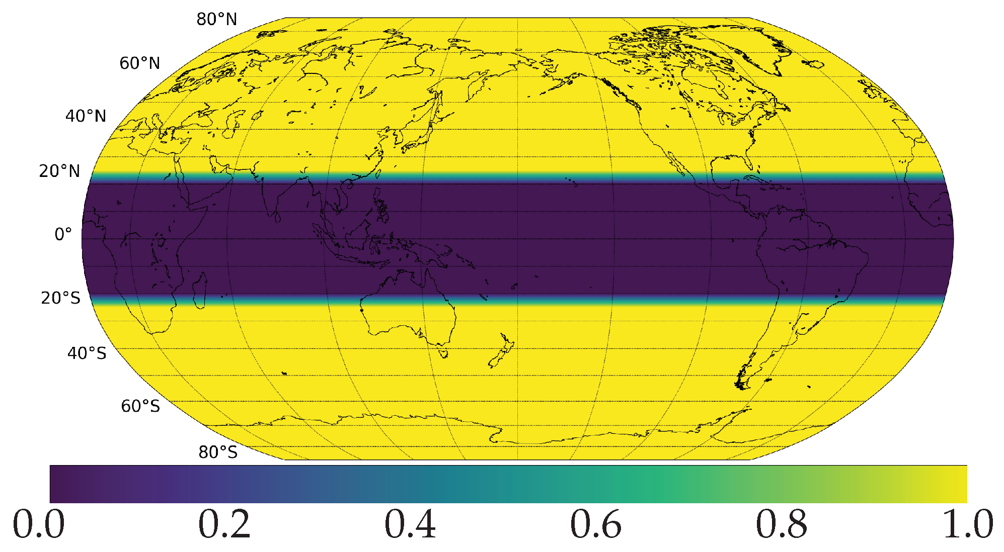
where is spatially varying and is depicted in Figure 4.
Equation (1) evaluated at gives an initial SST field of
which is the SST from NEMO in the tropics and the SST from OSTIA in the extratropics. For WCDA, we have therefore chosen to align the SST in the analysis with that used to initialise the forecast, i.e., following Equation (2).
3. Experimental Setup
A set of two experiments were conducted: the first is a control which does not use weakly coupled assimilation, and the second is an experiment with weakly coupled assimilation. Both experiments are based on IFS cycle 45R1. They were run at a 9 km global resolution (TCo1279), and both used the same uncoupled atmospheric EDA. The time period of the investigation is from 9 June 2017 to 21 May 2018. From each analysis, a 10-day coupled ocean–atmosphere forecast is produced.
3.1. Control—Uncoupled Assimilation
The initial conditions for the ocean component were taken from an ocean-only analysis, which takes its forcing fields from the operational HRES system, i.e., the same resolution but atmosphere only and driven by OSTIA boundary conditions. The atmospheric analysis used OSTIA SST and CI fields globally as its lower-boundary conditions.
3.2. Experiment—WCDA
An ocean analysis was run alongside the atmospheric analysis. The sea ice concentration field used for the lower boundary of the atmospheric analysis comes from the ocean analysis. Similarly, the sea-surface temperature field comes from the ocean analysis, although this is restricted to the tropics only, as described in Equation (2) and Figure 4. That is, the SST comes from the ocean analysis between 20 S and 20 N, OSTIA outside of 25 N(S), and a linear interpolation of the two in the 5 band from 20 N(S) to 25 N(S).
The atmospheric analysis is otherwise identical to the control run. Similarly, except for the forcing fields coming from the atmospheric analysis rather than the operational HRES system, the ocean analysis is identical to the ocean analysis used in the control experiment. A comparison of the WCDA experiment and the uncoupled control setup is shown in Figure 5.
4. Results and Discussion
For brevity, we show normalised differences in root-mean-square error (RMSE) as a measure of forecast errors [42]. Normalised RMSE differences (dRMSE) for an experiment e compared with a control experiment c is defined as
where and refer to forecasts of length t and analyses valid at time , and the norm is the root mean square throughout the number of samples through time.
4.1. Atmospheric Performance
Figure 6 shows the impact of WCDA on atmospheric humidity and temperature. There are three distinct regions of impact—the tropics and the poles—coming from the separate influences of WCDA through tropical SST and CI, respectively. The areas of hashed shading indicate that the differences in forecast errors are statistically significant. It is clear that the impact of WCDA does not have long-range impacts on the upper troposphere or on the spatial regions where WCDA is not active.
In the tropical region of Figure 6, we can see that the impact of the tropical SST is detected from the surface up to around 850 hPa in both temperature and humidity. The hashed shading shows that these improvements, indicated by blue colours, are statistically significant. The maps in Figure 7 show clearly that the improvement from SST is restricted to the latitudinal band for which the WCDA SST is active. Within this band, there are variations in how much benefit we get from WCDA. For instance, with the temperature at 1000 hPa, the strongest positive impacts are seen in the Arabian Sea, the Eastern Atlantic and Eastern Pacific (associated with cold tongues [43]).
In the Arabian Sea, there is evidence of improvement in other variables, such as in low-level winds and significant wave heights (not shown). This indicates that the SST WCDA has improved the position of the summer monsoon, which is known to be difficult to forecast well. The regions of positive impact in the Atlantic and the equatorial Pacific are regions that tend to have high cloud cover. This persistent cloud makes observing the SST from satellites difficult, and so it may be that the use of the ocean model within the OCEAN5 analysis system is able to effectively fill the observational gap.
In the polar regions, we see significant improvements in forecast errors due to the weakly coupled assimilation. Figure 8 and Figure 9 show that the improvements due to sea ice encompass the entire extent of the sea ice cover and are not simply confined to the ice edge. The areas of negative forecast impact in the sea ice variables (final row in Figure 8 and Figure 9) are likely an artefact of the mask used to compute these scores. In regions where both the analysis and forecast have no sea ice concentration, the forecast errors are identically zero. Hence, in the case where the control has a smaller extent than the experiment, we can find artificially high negative scores around the ice edge, which is what is seen in Figure 8 and Figure 9.
The small region of negative impact seen in humidity around 80 S (Figure 6a) is restricted to the areas around the Ross Ice Shelf and the Filchner-Ronne Ice Shelf (Figure 8, second row). The zonally averaged diagnostics give disproportionately large weight to areas at high latitudes. These ice shelves are mainly outside the domain of the ocean model which is currently used, and so interpolation between the ocean grid and the atmospheric grid is delicate in this area. Before operational implementation, a modified interpolation scheme was developed for this area to eliminate this negative signal.
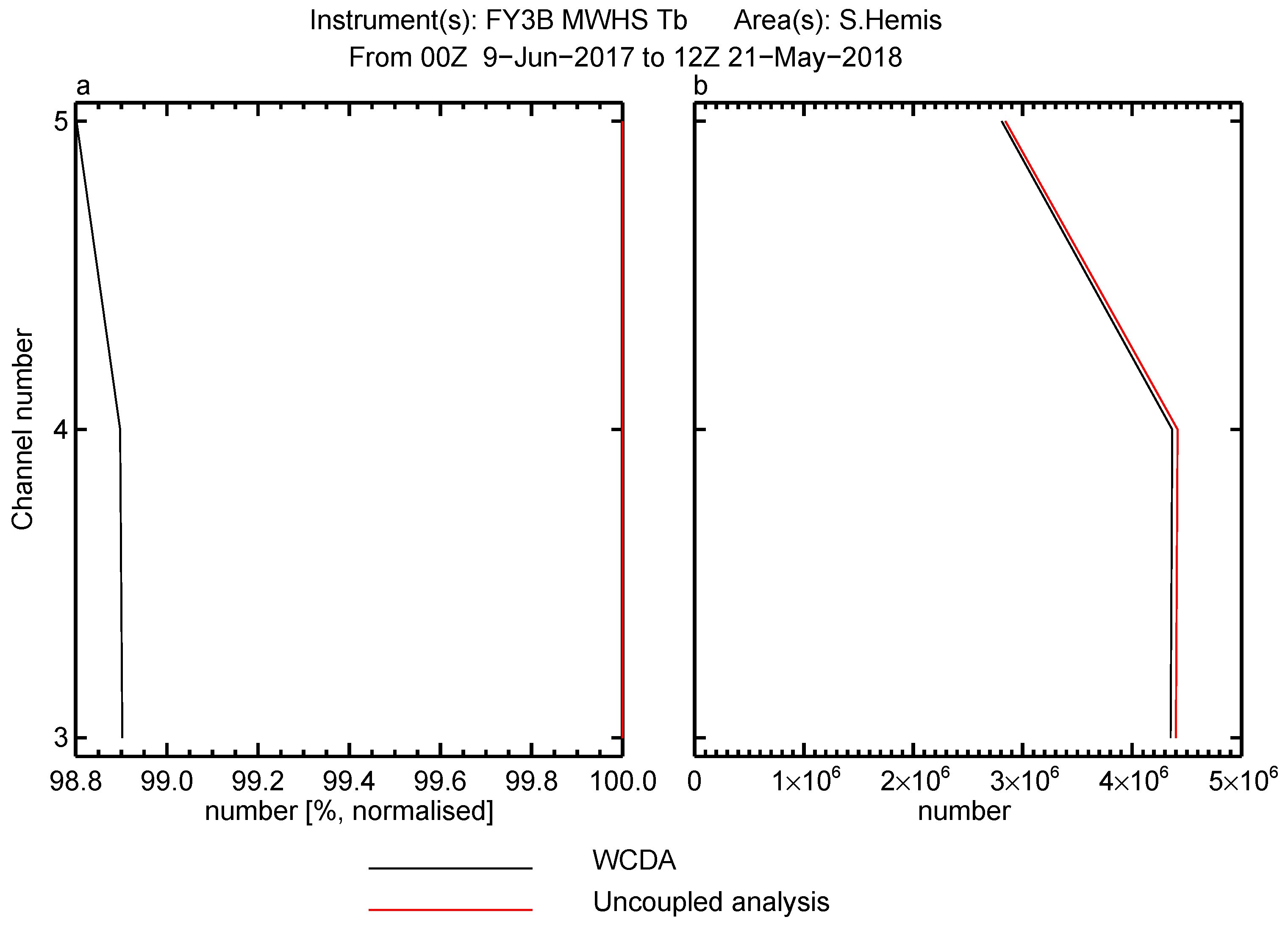
The influence of the WCDA CI extends up to roughly 700 hPa (Figure 6). This is further vertically than the impact of SST seen in the tropics. This can be explained by considering Figure 10, which shows the usage of microwave humidity soundings in the southern hemisphere. Such soundings are rejected over sea ice, and rejecting more contaminated soundings could lead to a more consistent atmospheric state in these regions. Further area-averaged dRMSEs of forecast error are shown in Appendix A.
4.2. Ocean Performance
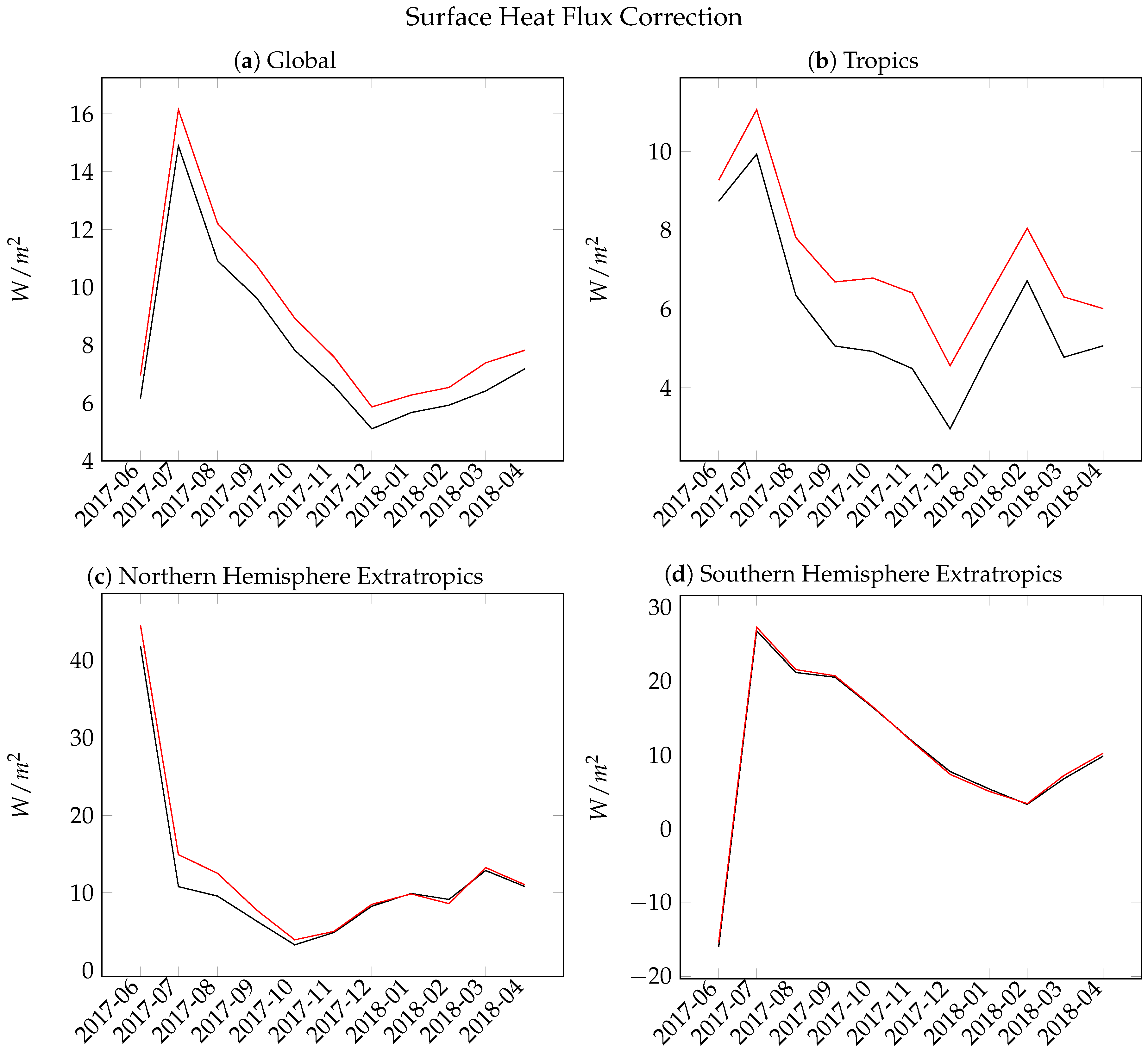
Figure 11 shows the area average of the heat flux correction, , used in the ocean analyses, which is defined as
where is a globally uniform restoration term of −200 WmK. This heat flux correction is applied to the surface non-solar heat flux. This flux correction represents the strength of the relaxation toward the OSTIA SST product. One can see that the flux correction in the extratropics is broadly similar in both experiments, with only the northern hemisphere extratropics showing a slightly smaller flux correction in July and August in the WCDA experiment. In the tropics, the flux correction is consistently substantially smaller in WCDA than in the uncoupled. This shows that the SST coupling in the tropics is leading to an SST field that is more consistent than the uncoupled analysis, requiring less corrections. We postulate that this could be due to the improved timeliness of the the SST that the atmospheric component uses (for the uncoupled analysis, the OSTIA SST field is only available on the day after its valid time); however, this requires a more detailed investigation that is outside the scope of this paper.
Figure 12 shows the area-averaged surface temperature increments in the ocean from the uncoupled and weakly coupled assimilation experiments. Similar to Figure 11, the larger benefits from WCDA appear to be seen in the tropics with the coupling of SST, showing reduced increments compared with the uncoupled analysis. However, in the northern hemisphere extratropics, the weakly coupled assimilation increments are consistently smaller than the increments in the uncoupled system. For the southern hemisphere extratropics, the picture is mixed, and it seems like the two systems are behaving very similarly.
4.3. Operational Impacts—Baltic Sea Detailed Sea Ice Investigation
Here, we take a detailed look at the spatial distribution of sea ice in the Baltic Sea, a particularly challenging area for sea ice concentration analyses. We show results for 2 separate days, as this is sufficient to highlight the behaviour of the different sea ice products in various scenarios throughout the winter season. Figure 13 shows different representations of the sea ice on 17 February 2018 from different sources. Figure 13a is a manually produced ice chart from FMI/SMHI showing sea ice concentration at the north of the Gulf of Bothnia, as well as in the eastern end of the Gulf of Finland. Figure 13b shows the available OSI SAF L3 sea ice concentration observations in the area. Note that because of the geography of the area, observations are only available in the centre of the Gulfs; coastal contamination requires that those points near the coast be masked from the product.
Figure 13c,d show the sea ice from uncoupled assimilation and WCDA experiments. One can see that the uncoupled analysis effectively smooths out the L3 observations and does not capture the high ice concentrations along the northern coastlines. WCDA, on the other hand, does a much better job at capturing the structures seen in the manual ice chart. In particular, the use of the background information coming from the dynamical model gives a much more realistic spatial distribution of the ice field. Figure 14 is similar but on 5 March 2018, the date of maximal sea ice extent in the Baltic Sea for the 2017/2018 season.
5. Conclusions and Future Plans
This study investigated the impact of weakly coupled ocean–atmosphere data assimilation on the ECMWF forecasts. The WCDA approach allows components of the Earth system with different timescales and assimilation methods to be linked together. As an alternative to using purely observation-based L4 products for the lower boundary of the atmosphere, with their associated latencies, WCDA allows dynamical models of the ocean and sea ice to fill the gaps in observations and propagate fields to the appropriate time. The results presented show that the use of WCDA improves the coupled forecasts in the regions near the interface of the variables being coupled.
In particular, it was shown that near-surface temperatures and humidities have smaller forecast errors in the WCDA system than the control experiment. Due to changes in the sea ice field, it was shown that the usage of satellite microwave sounder data within 4D-Var changes, as this data is screened based on the presence of sea ice. Statistics from the ocean analyses were compared and showed reduced analysis increments in the WCDA system, an indication of a more consistent analysis.
ECMWF’s operational upgrade to cycle 45R1 in June 2018 saw the introduction of WCDA through sea ice concentration. The forthcoming upgrade to cycle 46R1 is scheduled to also couple tropical SST, as per the experiments shown in this paper.
In addition to surface temperature and ice concentration information, the ocean analysis system can provide surface current information. Surface currents can be important for the assimilation of scatterometer data. Scatterometers measure the backscattering coefficient of the ocean surface. This coefficient is a function of wind velocity relative to the ocean current. In the current usage of scatterometers at ECMWF, we assume zero ocean currents, and so a WCDA system that has knowledge of the ocean currents should be able to make better use of scatterometer data.
There is plenty of scope to improve the partial coupling approach and its geospatial structure that determines the extent of SST coupling in the WCDA system. At the moment, it is a simple function of latitude. It may be beneficial for this to be basin dependent. Given the model biases in the western boundary currents, it may be beneficial to differ in the west and east of each basin.
These are the first steps in operational coupled ocean–atmosphere assimilation at ECMWF. A progressive approach toward implementation has been adopted rather than introducing coupling in all variables in a single system upgrade. This weakly coupled data assimilation system is flexible and could be applied in areas other than NWP, such as reanalysis. Whilst the weakly coupled approach is being developed, in parallel, the outer loop coupling approach is being explored as a possible operational system which would have a more immediate impact across the various Earth system components.
Author Contributions
Conceptualization, P.A.B., P.d.R.; software, P.A.B., H.Z., A.B., A.D.; writing—original draft preparation, P.A.B.; writing—review and editing, P.A.B., P.d.R., H.Z., A.B., A.D.
Funding
This research received no external funding.
Acknowledgments
We are grateful to Patrick Eriksson of FMI for providing assistance with the FMI/SMHI sea ice charts. Our thanks go to Magdalena Balmaseda, Stephen English, Sarah Keeley, and Kristian Mogensen for their help with implementations and insightful discussion of results.
Conflicts of Interest
The authors declare no conflict of interest.
Appendix A. Area-Averaged dRMSE of Forecast Errors
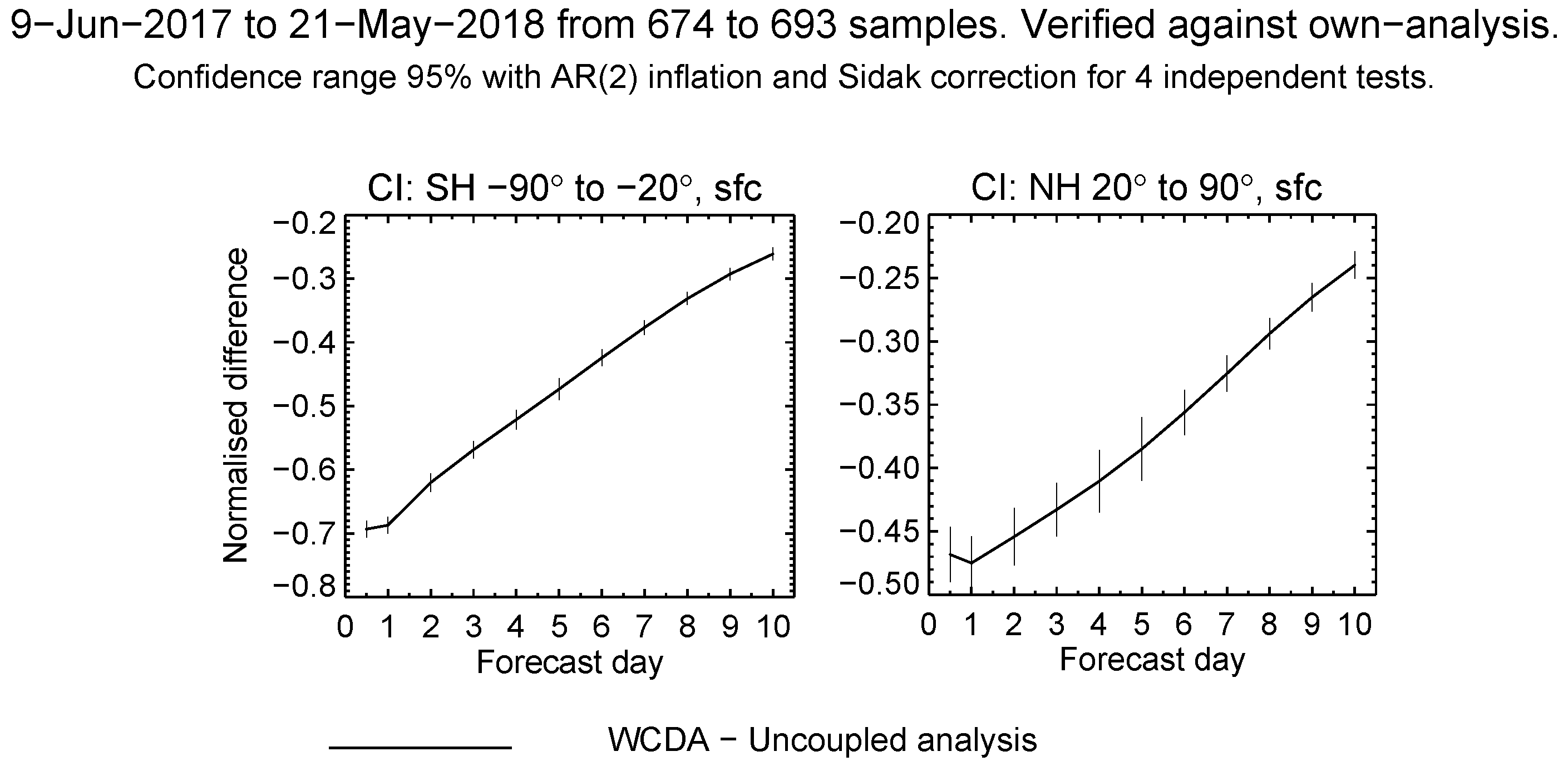
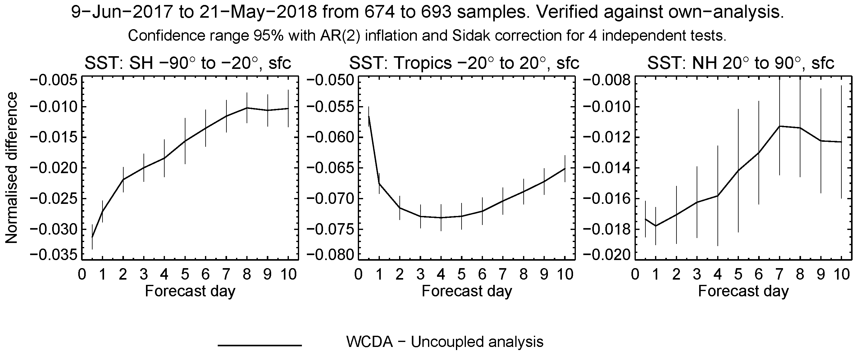
Figure A1.
Area-averaged diagram of the normalised difference in RMSE between WCDA and the control for sea ice concentration in the southern hemisphere (left), tropics (centre) and northern hemisphere (right) for forecasts at lead times of up to 10 days.
Figure A1.
Area-averaged diagram of the normalised difference in RMSE between WCDA and the control for sea ice concentration in the southern hemisphere (left), tropics (centre) and northern hemisphere (right) for forecasts at lead times of up to 10 days.

Figure A2.
As in Figure A1 but for sea-surface temperature.
Figure A2.
As in Figure A1 but for sea-surface temperature.

Figure A3.
As in Figure A1 but for atmospheric 2-m temperature.
Figure A3.
As in Figure A1 but for atmospheric 2-m temperature.

Figure A4.
As in Figure A1 but for atmospheric relative humidity and stratified by level, 100 hPa (top row), 500 hPa (second row), 850 hPa (third row) and 1000 hPa (bottom row).
Figure A4.
As in Figure A1 but for atmospheric relative humidity and stratified by level, 100 hPa (top row), 500 hPa (second row), 850 hPa (third row) and 1000 hPa (bottom row).

Figure A5.
As in Figure A4 but for atmospheric temperature.
Figure A5.
As in Figure A4 but for atmospheric temperature.

References
- ECMWF. The Strength of a Common Goal: A Roadmap to 2025; Technical Report; ECMWF: Reading, UK, 2016. [Google Scholar]
- Bauer, P.; Thorpe, A.; Brunet, G. The quiet revolution of numerical weather prediction. Nature 2015, 525, 47–55. [Google Scholar] [CrossRef] [PubMed]
- Maclachlan, C.; Arribas, A.; Peterson, K.A.; Maidens, A.; Fereday, D.; Scaife, A.A.; Gordon, M.; Vellinga, M.; Williams, A.; Comer, R.E.; et al. Global Seasonal forecast system version 5 (GloSea5): A high-resolution seasonal forecast system. Q. J. R. Meteorol. Soc. 2015, 141, 1072–1084. [Google Scholar] [CrossRef]
- Stockdale, T.N.; Anderson, D.L.; Alves, J.O.; Balmaseda, M.A. Global seasonal rainfall forecasts using a coupled ocean-atmosphere model. Nature 1998, 392, 370–373. [Google Scholar] [CrossRef]
- Vitart, F. Monthly Forecasting at ECMWF. Mon. Weather Rev. 2004, 132, 2761–2779. [Google Scholar] [CrossRef]
- Balmaseda, M.A.; Mogensen, K.; Weaver, A.T. Evaluation of the ECMWF ocean reanalysis system ORAS4. Q. J. R. Meteorol. Soc. 2013, 139, 1132–1161. [Google Scholar] [CrossRef]
- Bauer, P.; Richardson, D. New Model Cycle 40r1; ECMWF Newsletter No. 138, Winter 2013/2014; ECMWF: Reading, UK, 2014; p. 3. [Google Scholar]
- Rahmstorf, S. Climate drift in an ocean model coupled to a simple, perfectly matched atmosphere. Clim. Dyn. 1995, 11, 447–458. [Google Scholar] [CrossRef]
- Mulholland, D.P.; Laloyaux, P.; Haines, K.; Alonso Balmaseda, M. Origin and Impact of Initialization Shocks in Coupled Atmosphere-Ocean Forecasts. Mon. Weather Rev. 2015, 143, 4631–4644. [Google Scholar] [CrossRef]
- Sugiura, N.; Awaji, T.; Masuda, S.; Mochizuki, T.; Toyoda, T.; Miyama, T.; Igarashi, H.; Ishikawa, Y. Development of a four-dimensional variational coupled data assimilation system for enhanced analysis and prediction of seasonal to interannual climate variations. J. Geophys. Res. Oceans 2008, 113, 1–21. [Google Scholar] [CrossRef]
- Masuda, S.; Philip Matthews, J.; Ishikawa, Y.; Mochizuki, T.; Tanaka, Y.; Awaji, T. A new Approach to El Niño Prediction beyond the Spring Season. Sci. Rep. 2015, 5, 1–9. [Google Scholar] [CrossRef]
- Mochizuki, T.; Masuda, S.; Ishikawa, Y.; Awaji, T. Multiyear climate prediction with initialization based on 4D-Var data assimilation. Geophys. Res. Lett. 2016, 43, 3903–3910. [Google Scholar] [CrossRef] [Green Version]
- Yang, X.; Rosati, A.; Zhang, S.; Delworth, T.L.; Gudgel, R.G.; Zhang, R.; Vecchi, G.; Anderson, W.; Chang, Y.S.; DelSole, T.; et al. A predictable AMO-like pattern in the GFDL fully coupled ensemble initialization and decadal forecasting system. J. Clim. 2013, 26, 650–661. [Google Scholar] [CrossRef]
- Zhang, S.; Chang, Y.S.; Yang, X.; Rosati, A. Balanced and coherent climate estimation by combining data with a biased coupled model. J. Clim. 2014, 27, 1302–1314. [Google Scholar] [CrossRef]
- Saha, S.; Moorthi, S.; Wu, X.; Wang, J.; Nadiga, S.; Tripp, P.; Behringer, D.; Hou, Y.T.; Chuang, H.Y.; Iredell, M.; et al. The NCEP climate forecast system version 2. J. Clim. 2014, 27, 2185–2208. [Google Scholar] [CrossRef]
- Saha, S.; Moorthi, S.; Pan, H.L.; Wu, X.; Wang, J.; Nadiga, S.; Tripp, P.; Kistler, R.; Woollen, J.; Behringer, D.; et al. The NCEP climate forecast system reanalysis. Bull. Am. Meteorol. Soc. 2010, 91, 1015–1057. [Google Scholar] [CrossRef]
- Penny, S.G.; Akella, S.; Alves, O.; Bishop, C.; Buehner, M.; Chevallier, M.; Counillon, F.; Draper, C.; Frolov, S.; Fujii, Y.; et al. Coupled Data Assimilation for Integrated Earth System Analysis and Prediction: Goals, Challenges and Recommendations; Technical Report; World Meteorological Organisation: Geneva, Switzerland, 2017. [Google Scholar]
- Frolov, S.; Bishop, C.H.; Holt, T.; Cummings, J.; Kuhl, D. Facilitating Strongly Coupled Ocean-Atmosphere Data Assimilation with an Interface Solver. Mon. Weather Rev. 2016, 144, 3–20. [Google Scholar] [CrossRef]
- Lea, D.J.; Mirouze, I.; Martin, M.J.; King, R.R.; Hines, A.; Walters, D.; Thurlow, M. Assessing a New Coupled Data Assimilation System Based on the Met Office Coupled Atmosphere–Land–Ocean–Sea Ice Model. Mon. Weather Rev. 2015, 143, 4678–4694. [Google Scholar] [CrossRef]
- Laloyaux, P.; Balmaseda, M.; Dee, D.; Mogensen, K.; Janssen, P. A coupled data assimilation system for climate reanalysis. Q. J. R. Meteorol. Soc. 2016, 142, 65–78. [Google Scholar] [CrossRef]
- Schepers, D.; Boisséson, E.D.; Eresmaa, R.; Lupu, C.; Rosnay, P.D. CERA-SAT: A coupled satellite-era reanalysis. ECMWF Newslett. 2018, 155, 32–37. [Google Scholar] [CrossRef]
- ECMWF. Part III: Dynamics and numerical procedures. In IFS Documentation CY43R3; Number 3 in IFS Documentation; ECMWF: Reading, UK, 2017. [Google Scholar]
- ECMWF. Part IV: Physical processes. In IFS Documentation CY43R3; Number 4 in IFS Documentation; ECMWF: Reading, UK, 2017. [Google Scholar]
- Balsamo, G.; Beljaars, A.; Scipal, K.; Viterbo, P.; van den Hurk, B.; Hirschi, M.; Betts, A.K. A Revised Hydrology for the ECMWF Model: Verification from Field Site to Terrestrial Water Storage and Impact in the Integrated Forecast System. J. Hydrometeorol. 2009, 10, 623–643. [Google Scholar] [CrossRef]
- Dutra, E.; Stepanenko, V.M.; Balsamo, G.; Viterbo, P.; Miranda, P.M.A.; Mironov, D.; Schär, C. Impact of Lakes on the ECMWF Surface Scheme. In ECMWF Technical Memorandum; ECMWF: Reading, UK, 2009; pp. 1–15. [Google Scholar]
- ECMWF. Part VII: ECMWF wave model. In IFS Documentation CY43R3; Number 7 in IFS Documentation; ECMWF: Reading, UK, 2017. [Google Scholar]
- Rabier, F.; Järvinen, H.; Klinker, E.; Mahfouf, J.F.; Simmons, A. The ECMWF operational implementation of four-dimensional variational assimilation. Part I: Experimental results and diagnostics wiht operational configuration. Q. J. R. Meteorol. Soc. 2000, 126, 1143–1170. [Google Scholar] [CrossRef]
- De Rosnay, P.; Balsamo, G.; Albergel, C.; Muñoz-Sabater, J.; Isaksen, L. Initialisation of Land Surface Variables for Numerical Weather Prediction. Surv. Geophys. 2014, 35, 607–621. [Google Scholar] [CrossRef]
- English, S.; McNally, A.; Borman, N.; Salonen, K.; Matricardi, M.; Horányi, A.; Rennie, M.; Janisková, M.; Di Michele, S.; Geer, A.; et al. Impact of Satellite Data. In Technical Memoradum ECMWF; ECMWF: Reading, UK, 2013; p. 46. [Google Scholar]
- Haiden, T.; Dahoui, M.; Ingleby, B.; Rosnay, P.D.; Prates, C.; Kuscu, E.; Hewson, T.; Isaksen, L.; Richardson, D.; Zuo, H.; Jones, L. Use of In Situ Surface Observations at ECMWF. In Technical Memoradum ECMWF; ECMWF: Reading, UK, 2018. [Google Scholar]
- Donlon, C.J.; Martin, M.; Stark, J.; Roberts-Jones, J.; Fiedler, E.; Wimmer, W. The Operational Sea Surface Temperature and Sea Ice Analysis (OSTIA) system. Remote Sens. Environ. 2012, 116, 140–158. [Google Scholar] [CrossRef]
- OSI SAF. OSI-401-b. Available online: http://www.osi-saf.org/?q=content/global-sea-ice-concentration-ssmis (accessed on 14 January 2019).
- NCEP. MMAB Sea Ice Analysis. Available online: http://polar.ncep.noaa.gov/seaice/Analyses.shtml (accessed on 14 January 2019).
- Bonavita, M.; Isaksen, L.; Hólm, E. On the use of EDA background error variances in the ECMWF 4D-Var. Q. J. R. Meteorol. Soc. 2012, 138, 1540–1559. [Google Scholar] [CrossRef] [Green Version]
- Haseler, J. The Early-Delivery Suite; Technical Memorandum 454; ECMWF: Reading, UK, 2004. [Google Scholar]
- Zuo, H.; Balmaseda, M.A.; Tietsche, S.; Mogensen, K.; Mayer, M. The ECMWF operational ensemble reanalysis-analysis system for ocean and sea-ice: A description of the system and assessment. Ocean Sci. Discuss. 2019. under review. [Google Scholar] [CrossRef]
- Zuo, H.; Balmaseda, M.A.; Mogensen, K.; Tietsche, S. OCEAN5: The ECMWF Ocean Reanalysis System and Its Real-Time Analysis Component; Technical Report 823; ECMWF: Reading, UK, 2018. [Google Scholar]
- ECMWF. Part V: Ensemble prediction system. In IFS Documentation CY40R1; Number 5 in IFS Documentation; ECMWF: Reading, UK, 2014. [Google Scholar]
- Mogensen, K.; et al. The ECMWF Coupled Atmosphere-Wave-Ocean-Ice Model as Implemented in CY45R1: Part 1: Technical Implementation. In ECMWF Technical Memorandum; ECMWF: Reading, UK, 2019; in prep. [Google Scholar]
- Mogensen, K.; et al. The ECMWF Coupled Atmosphere-Wave-Ocean-Ice Model as Implemented in CY45R1: Part 2: Ocean Model Performance. In ECMWF Technical Memorandum; ECMWF: Reading, UK, 2019; in prep. [Google Scholar]
- Keeley, S.; et al. The ECMWF Coupled Atmosphere-Wave-Ocean-Ice Model as Implemented in CY45R1: Part 3: Ice model performance. In ECMWF Technical Memorandum; ECMWF: Reading, UK, 2019; in prep. [Google Scholar]
- Geer, A.J. Significance of changes in medium-range forecast scores. Tellus A 2016, 68, 1–21. [Google Scholar] [CrossRef]
- Siedler, G.; Gould, J.; Church, J. Ocean Circulation and Climate: Observing and Modelling the Global Ocean; International Geophysics, Elsevier Science: Amsterdam, The Netherlands, 2001. [Google Scholar]
- FMI; SMHI. Baltic sea ice chart. Available online: http://cdn.fmi.fi/marine-observations/products/ice-charts/20180217-full-color-ice-chart.pdf (accessed on 10 July 2018).
Figure 1.
Components of the European Centre for Medium-Range Weather Forecasts’ (ECMWF’s) Integrated Forecasting System (IFS) Earth system. Along with the atmosphere, there are the ocean, wave, sea ice, land surface and lake models.
Figure 1.
Components of the European Centre for Medium-Range Weather Forecasts’ (ECMWF’s) Integrated Forecasting System (IFS) Earth system. Along with the atmosphere, there are the ocean, wave, sea ice, land surface and lake models.

Figure 2.
Impact of first implementation of outer loop coupling (quasi strongly coupled data assimilation) on high-resolution global numerical weather prediction (NWP). The presence of model bias in the western boundary currents of the ocean is evident as degradations (red) to the 24 h forecast scores of vector winds (VW) at 1000 hPa. Results were obtained from IFS cycle 45R1 at a resolution of 25 km (TCo399) with a ocean and are based on global outer loop coupling over the period from 1 June 2017 to 2 July 2017. See Section 4 for details of the error diagnostic.

Figure 3.
Weakly coupled assimilation system information flow. Horizontal bars represent the analysis window for the various different components of the system. This is a simplified plot ignoring a 3 h offset of the systems. Orange arrows show the existing transfer of forcing from the atmosphere to the ocean. Magenta arrows show the addition using the OCEAN5 fields as the lower-boundary condition for the atmospheric analysis, thus forming the weakly coupled data assimilation (WCDA) system. The highlighted region is discussed in an example in the text.

Figure 4.
coefficient from Equation (1b) indicating that initial sea-surface temperature (SST) is taken from the ocean analysis in the tropics (from 20 S to 20 N) and from Operational Sea Surface Temperature and Sea Ice Analysis (OSTIA) in the extratropics. The transition regions can be seen as the bands consisting of intermediate colours.

Figure 5.
Schematic of experimental design. On the right is the experiment, with the weakly coupled DA passing information between atmosphere and ocean analyses. On the left is the control atmospheric analysis getting its SST and sea ice concentration (CI) from the external OSTIA product, with the forcing field for the control ocean analysis coming from the operational HRES system.

Figure 6.
Latitude–pressure diagram of the zonally averaged normalised difference in root-mean-square error (RMSE) between WCDA and the control for humidity (top) and temperature (bottom) forecasts at 12 h (left) and 24 h (right) lead times, for the period from 9 June 2017 to 21 May 2018. Hashed areas indicate statistically significant differences.

Figure 7.
Spatial maps of the normalised difference in RMSE between WCDA and the control for temperature at 1000 hPa (top), skin temperature (middle) and sea-surface temperature (bottom) forecasts at 12 h (left) and 120 h (right) lead times (48 h lead time for temperature at 1000 hPa), for the period from 9 June 2017 to 21 May 2018.

Figure 8.
Spatial maps centred on the Antarctic of the normalised difference in RMSE between WCDA and the control for 1000 hPa temperature (top), 1000 hPa humidity (middle) and sea ice concentration (bottom) forecasts at 12 h (left) and 24 h (right) lead times (120 h lead time for sea ice concentration), for the period 9 June 2017 to 21 May 2018.

Figure 9.
Similar to Figure 8 but focused on the Arctic.
Figure 9.
Similar to Figure 8 but focused on the Arctic.

Figure 10.
Observation usage of MWHS-1 in the southern hemisphere for the WCDA experiment (black) and the uncoupled control (red). Figure (a) shows the normalised observation usage and figure (b) shows the absolute numbers.
Figure 10.
Observation usage of MWHS-1 in the southern hemisphere for the WCDA experiment (black) and the uncoupled control (red). Figure (a) shows the normalised observation usage and figure (b) shows the absolute numbers.

Figure 11.
Monthly averaged ocean heat flux correction from the uncoupled analysis (red) and the weakly coupled analysis (black). This is split by region showing global (top left), the tropics (top right), the northern hemisphere extratropics (bottom left) and the southern hemisphere extratropics (bottom right).

Figure 12.
As in Figure 11 but for surface assimilation temperature increments.
Figure 12.
As in Figure 11 but for surface assimilation temperature increments.

Figure 13.
(a) Manually produced Finnish–Swedish ice chart of the Baltic Sea. © [44] Reproduced with permission. (b) OSI SAF 401-b product. Note missing data (grey) around coastlines due to coastal contamination in satellite retrievals of sea ice concentration. (c) Uncoupled analysis. Note the Gaussian nature of the ice field centred on the available OSI SAF L3 observations. (d) WCDA. Note the much more realistic structure and the good agreement with the manual ice chart. A manual ice chart (a) and sea ice concentration values in the Baltic sea on 17 February 2018 from OSI SAF L3 observations (b), uncoupled analysis (c) and WCDA (d).

Figure 14.
(a) Manually produced Finnish–Swedish ice chart of the Baltic Sea. © [44] Reproduced with permission. (b) OSI SAF 401-b product. Note missing data (grey) around coastlines due to coastal contamination in satellite retrievals of sea ice concentration. (c) Uncoupled analysis. Note the Gaussian nature of the ice field centred on the available OSI SAF L3 observations. (d) WCDA. Note the much more realistic structure and the good agreement with the manual ice chart. As in Figure 13 but on 5 March 2018, the date of maximum sea ice extent in the region for the season.

© 2019 by the authors. Licensee MDPI, Basel, Switzerland. This article is an open access article distributed under the terms and conditions of the Creative Commons Attribution (CC BY) license (http://creativecommons.org/licenses/by/4.0/).
Share and Cite
MDPI and ACS Style
Browne, P.A.; de Rosnay, P.; Zuo, H.; Bennett, A.; Dawson, A. Weakly Coupled Ocean–Atmosphere Data Assimilation in the ECMWF NWP System. Remote Sens. 2019, 11, 234. https://doi.org/10.3390/rs11030234
AMA Style
Browne PA, de Rosnay P, Zuo H, Bennett A, Dawson A. Weakly Coupled Ocean–Atmosphere Data Assimilation in the ECMWF NWP System. Remote Sensing. 2019; 11(3):234. https://doi.org/10.3390/rs11030234
Chicago/Turabian StyleBrowne, Philip A., Patricia de Rosnay, Hao Zuo, Andrew Bennett, and Andrew Dawson. 2019. "Weakly Coupled Ocean–Atmosphere Data Assimilation in the ECMWF NWP System" Remote Sensing 11, no. 3: 234. https://doi.org/10.3390/rs11030234
Note that from the first issue of 2016, this journal uses article numbers instead of page numbers. See further details here.