Combining Satellite Imagery and Numerical Modelling to Study the Occurrence of Warm Upwellings in the Southern Baltic Sea in Winter


1
Institute of Marine and Environmental Sciences, University of Szczecin, 70-383 Szczecin, Poland
2
Institute of Oceanography, University of Gdańsk, 81-378 Gdynia, Poland
3
Institute of Oceanology of Polish Academy of Sciences, 81-712 Sopot, Poland
*
Author to whom correspondence should be addressed.
Remote Sens. 2019, 11(24), 2982; https://doi.org/10.3390/rs11242982
Submission received: 30 October 2019
/
Revised: 8 December 2019
/
Accepted: 9 December 2019
/
Published: 12 December 2019
(This article belongs to the Special Issue Remote Sensing Applications in Coastal Environment)
Abstract
:Coastal upwelling involves an upward movement of deeper, usually colder, water to the surface. Satellite sea surface temperature (SST) observations and simulations with a hydrodynamic model show, however, that the coastal upwelling in the Baltic Sea in winter can bring warmer water to the surface. In this study, the satellite SST data collected by the advanced very high resolution radiometer (AVHRR) and the moderate-resolution imaging spectroradiometer (MODIS), as well as simulations with the Parallel Model 3D (PM3D) were used to identify upwelling events in the southern Baltic Sea during the 2010–2017 winter seasons. The PM3D is a three-dimensional hydrodynamic model of the Baltic Sea developed at the Institute of Oceanography, University of Gdańsk, Poland, in which parallel calculations enable high-resolution modelling. A validation of the model results with in situ observations and satellite-derived SST data showed the PM3D to adequately represent thermal conditions in upwelling areas in winter (91.5% agreement). Analysis of the frequency of warm upwellings in 12 areas of the southern Baltic Sea showed a high variability in January and February. In those months, the upwelling was most frequent, both in satellite imagery and in model results, off the Hel Peninsula (38% and 43% frequency, respectively). Upwelling was also frequent off the Vistula Spit, west of the Island of Rügen, and off the eastern coast of Skåne, where the upwelling frequency estimated from satellite images exceeded 26%. As determined by the PM3D, the upwelling frequency off VS and R was at least 25%, while off the eastern coast of Skåne, it reached 17%. The faithful simulation of SST variability in the winters of 2010–2017 by the high-resolution model used was shown to be a reliable tool with which to identify warm upwellings in the southern Baltic Sea.
1. Introduction
Upwelling is recorded in many coastal areas of seas and oceans and even in large lakes. It involves a vertical upward transport of near-bottom water masses to the surface [1]. According to the Ekman theory, upwelling in the northern hemisphere can occur when the current moves along the shore situated to the left of the velocity vector. The upwelled water is frequently different in its physical and chemical properties from the surface water. Therefore, in a thermally stratified sea, such as the Baltic Sea, the occurrence of an upwelling can be inferred not only from in situ measurements, but also from satellite imagery [2,3]. Studies carried out in the summer showed upwelling to be an important process affecting water mixing and coastal weather [4,5,6,7]. The upwelled water is usually nutrient-rich; therefore, upwelling affects primary production and the phytoplankton biomass [6,8,9,10,11].
The Baltic Sea is a shallow intracontinental sea of the Atlantic Ocean (Figure 1). It is a semi-enclosed water body with a surface area of 392,978 km2 and a 54 m mean depth [12]. The water temperature changes seasonally. During spring, the water column temperature profile shows a thermocline which separates the warm upper layer from the cooler intermediate water. This thermocline impedes vertical mixing within the upper layer until late autumn [13]. During that time, under an appropriate wind regime, the emergence of an upwelling may result in a rapid temperature drop by as much as more than 10 °C [10]. In winter, when the surface temperature decreases, the effects of warmer upwelled water are visible as the surface temperature increases. Off the southern coasts of the Gulf of Finland, the surface temperature may then raise to 3.5–4 °C [14].
The increasing use of satellite-based remote sensing, in progress since the early 1980s, has made it possible to detect upwellings in the Baltic Sea, not only from direct in situ measurements, but also through satellite-based records of the surface temperature [2,15,16,17,18,19]. At present, there is a variety of remote techniques with which to detect upwellings [11,20,21,22,23,24].
A thermal infrared remote sensing-based analysis of upwellings is possible only at the absence of cloud cover, cloudiness over the Baltic Sea being usually quite considerable. As shown by Finkensieper et al. [25], in 2010–2015, the annual mean frequency of cloud cover over the Baltic Sea varied from 62.0% to 89.5%. Although passive microwave devices can be used when the cloudiness limits the use of infrared techniques, their resolution is too low in comparison to upwelling sizes to detect them. Therefore, upwelling hydrodynamics in different regions of the Baltic Sea has been addressed by many numerical studies, beginning with the 1990s research on modelling the upwelling off the Island of Rügen [26,27]. Subsequently, other numerical models describing upwelling in response to atmospheric and hydrological forcing have been developed [3,5,28,29,30,31,32]. In recent years, many studies addressed upwellings by using both satellite-based remote sensing and numerical modelling [6,7,33,34].
The summer coastal upwelling sites and frequency in the southern Baltic Sea are relatively well known. When studying upwellings off the western coast of the Island of Rügen and off the Polish coast, Horstmann [15] demonstrated the appearance of upwelling with easterly and southeasterly winds. Gidhagen [16], who analysed upwellings off the Swedish coast, found them to occur most frequently with winds from the western sector. Bychkova and Viktorov [4] identified 14 upwelling zones in the Baltic Sea proper. For each zone, they reported basic characteristics such as the upwelling size and typical wind regime. A more comprehensive list of upwelling sites throughout the Baltic Sea, depending on the atmospheric circulation type, was given by Bychkova et al. [17]. Myrberg and Andrejev [29], using an upwelling index based on the numerical computation of vertical velocity, attempted to calculate the frequency of upwellings throughout the Baltic Sea. They demonstrated that in the southern Baltic Sea, the upwelling frequency in some areas exceeds 30%. Based on the analysis of simulated vertical velocity, Kowalewski and Ostrowski [34] determined the upwelling frequency in 12 southern Baltic areas. They determined the frequency for every month in a year and identified conditions favourable for upwelling generation. Krężel et al. [2] assessed the size of upwelling off the Hel Peninsula, Kołobrzeg, and Łeba within areas of 1400, 5000, and 3500 km2, respectively. He pointed out that the temperature difference between surface and deep water often make it possible to trace the range and directions of the spreading upwelled water on satellite images for as long as ten days, sometimes even longer. Based on satellite imagery and numerical simulations, Lehmann et al. [6] showed that the upwelling frequency in May–September in some coastal areas of the Baltic Sea occasionally reached 40%. In the southern Baltic Sea, they observed upwellings to be particularly frequent off the coast of the Hanö Bay and off the southernmost coast of Sweden. Moreover, Lehmann et al. [6] demonstrated a positive trend of upwelling frequencies along the Swedish coast of the Baltic Sea and the Finnish coast of the Gulf of Finland as well as a negative trend along the Polish, Latvian and Estonian coasts. At the eastern coast of the southern Baltic Sea, several authors found that northerly winds make a significant contribution to upwelling generation [4,11,23,34].
While numerous studies have addressed problems associated with the detection of sites and frequency of summer upwellings in the Baltic Sea, there is a paucity of literature on upwelling sites and frequency in winter. This most likely stems from methodological differences. On the one hand, upwellings occur irregularly and their spatial and temporal scales are small; on the other, the dense cloud cover over the Baltic Sea in winter largely prevents the use of satellite information on the sea surface temperature (SST). The few studies addressing the problem relied primarily on results of in situ measurements. Svansson [35] documented the presence of winter upwelling off the east coast of Sweden (outside Västervik), whereas Suursaar [14] described the effect off the southern coast of the Gulf of Finland (near Sillamäe). Suursaar [14] observed, inter alia, that the occurrence of upwelling in winter produced a stronger record in water salinity and currents than in water temperature. The upwelling frequency of 12 areas of the southern Baltic in winter was determined based on numerical simulations of vertical velocities by Kowalewski and Ostrowski [34]. They found that in winter, as a result of the prevalence of westerly and southwesterly winds, upwellings off the east coast of Skåne are more frequent than downwelling. Along the Polish coastline, downwelling prevails. Off the Hel Peninsula, the frequencies of strong upwellings in January and February are 30% and 21%, respectively. Off the Hel Peninsula and off the Kołobrzeg, the probability was the highest when winds were from the southerly to northeasterly sectors. Off the Łeba, upwelling was generated mainly by the southeasterly to northeasterly winds. The only region on the southern coast of the Baltic with prevailing upwelling is the area off the Vistula Spit, in spite of prevailing westerly winds. In the eastern part of the southern Baltic, in winter, downwelling was more frequent than upwellings. It is noteworthy that the warm water transport by upwelling in winter and its effects on the marine environment have been studied so far primarily in Arctic areas [36,37,38]. In the opinion of Randelhoff and Sundfjord [39], in a strongly stratified sea such as the Beaufort Sea, should the upwelling frequency in winter increase in the future because of reduced sea ice cover, this can be an important factor contributing to the pre-bloom nutrient pool.
The present work was aimed at identifying sites and the frequency of upwelling in the southern Baltic Sea in winter based on the SST information acquired from the Advanced Very High-Resolution Radiometer (AVHRR) and the Moderate-Resolution Imaging Spectroradiometer (MODIS) and results of numerical simulations of a parallel, high spatial resolution version of the three-dimensional hydrodynamic model of the Baltic Sea (PM3D). The use of the PM3D was necessitated by a poor availability of satellite data due to a dense cloud cover observed above the Baltic Sea in winter. Upwelling events were identified in January and February of 2010–2017. Section 2 describes the area of interest, the data used for the upwelling detection, and the main features of the PM3D; it also specifies details of SST filtration and assimilation from the AVHRR and MODIS systems, from satellite maps available in the SatBałtyk System. This subsection closes with the description of validation methods. Section 3 presents results of validation of the simulated SST for 2010–2017 and analysis of concordance between numerical simulations and satellite observations in upwelling areas. The section analyses the winter upwelling frequency in the Baltic Sea and presents the representation of warm upwellings in different regions of the southern Baltic Sea. Discussion and concluding remarks bring the paper to a close.
2. Materials and Methods
2.1. The Area of Interest
The upwelling frequency in January and February of 2010–2017 was analysed based on model simulations using the PM3D and the available satellite imagery from the AVHRR and MODIS radiometers for 12 regions of the southern Baltic Sea (Table 1, Figure 1). The regions were identified based on the available literature [6,17,29,34] and on the analysis of upwelling generation sites indicated by the model.
2.2. Satellite Data
Upwelling detection was undertaken using satellite images registered by AVHRR/3 used by the NOAA (the National Oceanic and Atmospheric Administration) and METOP (Meteorological Operational Satellite) satellites as well as from MODIS mounted on the Terra and Aqua satellites. The data were acquired from the SatBałtyk System (http://satbaltyk.iopan.gda.pl) [40]. Until 2012, the AVHRR data were received at the University of Gdańsk via the HRPT Station (NOAA RAW High Resolution Picture Transmission data); then the data were downloaded from the EUMETCast system (NOAA RAW and MetOp Level-0) or from the EUMETSAT (European Organisation for the Exploitation of Meteorological Satellites) Archive (NOAA RAW and MetOp Level-1b). Instrumental correction and the calculation of the brightness temperature (AVHRR channels 4 and 5) were carried out in accordance with standard NOAA procedures using AAPP software [41]. Ice and cloud detection was performed using the MAIA 3 algorithm [42]. The cloud mask was extended further by a buffer of one pixel in width around clouds in order to hinder the influence of bad cloud masking. The bulk SST was computed according to the nonlinear split-window formula [43]. The AVHRR and MODIS data were provided several times a day at irregular intervals. They were georeferenced according to the procedure put forward by Kowalewski and Krężel [44] and reprojected into a 1 km grid in the Lambert Azimuthal Equal-Area projection used in the SatBałtyk system.
2.3. The Model
2.3.1. The Model Output
The three-dimensional hydrodynamic model of the Baltic Sea (M3D) has been used at the Institute of Oceanography, University of Gdańsk for more than twenty years. The model is based on the model of oceanic coastal circulation, known as the Princeton Ocean Model (POM) [45]. The POM was adapted to the Baltic Sea conditions by Kowalewski [46]. The operational version of the M3D became operational in 1999 [47]. The M3D was used then as a basis on which to build other modules, like the ProDeMo (Production and Destruction of Organic Matter Model) [48,49] or to model the sea ice thermodynamics and dynamics in the Baltic Sea [50]. Subsequent studies showed the M3D to be very useful for the analysis of physical processes in the coastal zone, including modelling thermal conditions at upwelling sites [34] as well as sea- and freshwater mixing during storm surges [51]. Within the framework of the project “The satellite monitoring of the Baltic Sea environment” (acronym: SatBałtyk) [52,53] dealing with remote sensing methods for monitoring of the Baltic Sea ecosystem, measures were taken to increase the M3D resolution to render it applicable to enhance SST maps in cloud-covered areas. As a result, a new version, the Parallel Model 3D (PM3D) was developed; parallel computations used by the model made it possible to increase the resolution to that achieved in satellite imagery [54]. This, in turn, facilitated development of an algorithm with which to complement information from the satellite SST imagery under cloudy conditions by using a mosaic of consecutive satellite maps together with numerical models as an additional source of information [40]. The PM3D assimilates the SST data retrieved from the AVHRR and MODIS radiometers, so its results do not differ significantly from those observed by satellite remote sensing. The PM3D has been already used to study the long-term variability of currents and circulation patterns in the Baltic Sea [55], as well as to storm surge prediction [54].
In the PM3D, calculations are conducted in parallel for two areas (computational domains) of different spatial resolution: 1 nautical mile (NM), i.e., 1.85 km for the Baltic Sea and the Skagerrak and 0.5 NM (about 0.9 km) for the southern part of the Baltic Sea. Simulation of a 24 h period is effected in 64 min [54]. Parallel calculations, which facilitate high-resolution SST modelling, have made it possible to use the PM3D while supplementing SST satellite maps in overcast areas without any loss of accuracy in the SatBałtyk System (http://satbaltyk.iopan.gda.pl/, [40]). A total of 18 layers in the sigma representation have been defined in the vertical plane [34].
The water exchange proceeds through the open boundary between the North Sea and the Skagerrak. The boundary involved a radiation marginal condition for flows, the sea level changes being introduced based on 1 h interval observation data for station Tregde (http://www.sjokart.no/en/sehavniva/). The model utilises meteorological data from the 4 km resolution operational weather Unified Model (UM) [56], the solar energy input is derived from the diagnostic SolRad model [57], and the monthly mean inflow of more than 150 river into the Baltic Sea is included (http://nest.su.se/bed/).
2.3.2. Filtration and Assimilation of SST Satellite Data from AVHRR and MODIS Radiometers
Data supplied by numerical models are always approximations. Errors are associated with model assumption which simplify the physical processes being modelled and thus allow one to solve the problem. As a result, it is necessary to correct modelling results by assimilation of observational data. Spatial SST distribution recorded by different satellites is a useful source of data for assimilation by hydrodynamic models. The major advantage of such data sets is a possibility to record, with a high resolution, temperature fields over large areas; another advantage is the rapidity with which such data are available. The major disadvantage of remotely sensed SST, especially in the Baltic Sea region, is the low accuracy on the order of 1 °C [40,58]. Another problem stems from the fact that the measurement pertains only to a very thin surface water layer. Despite the employment of procedure of skin temperature correction for the calculation of bulk SST, under certain conditions, a difference between the satellite-derived and conventionally measured SST may be quite large, on the order of a few degrees. This is the case, for instance, on windless sunny days when the absence of mixing allows the surface to be heated quite strongly. This phenomenon is called a hotspot. On the other hand, the cloud cover precludes SST recording by radiometers operating in the infra-red range. When a part of the sky area is overcast, satellite imagery—to be applicable—requires masking the clouds, which is not straightforward. Very thin clouds and fogs are difficult to identify and—when left unmasked—may render the SST underestimated. All those drawbacks of the satellite SST estimation do not rule it out for the correction of results of modelling but should be taken into account when developing a data assimilation method.
The assimilation of oceanographic data is usually effected with methods adapted from meteorology. One of the first methods for the objective analysis, a simple but numerically very effective, was proposed by Cressman [59]. The statistical method of optimal interpolation [60] produces the best linear unbiased field estimator. There have been numerous algorithms with which to solve a simplified version of the Kalman filter, including the Ensemble Kalman filter [61,62], the Singular Evolutive Extended Kalman filter [63], and the Singular Evolutive Interpolated Kalman filter [63]. An alternative approach involves an iteration-based solution of the cost function utilising variance-based methods such as the 3DVar and 4DVar [64]. Many of those methods were applied to hydrodynamic models of the Baltic Sea to assimilate both the point source and the satellite data [65,66,67,68,69].
When assimilating satellite imagery, the problem of spatial interpolation is of secondary importance because the spatial resolution of the images is similar to or better than the resolution of the models. As the resolution is similar to that of the model, no advanced interpolation techniques are necessary and the SST images are directly reprojected to the model grid by bilinear interpolation. In addition, the satellite images are uniformly distributed over the rectangular spatial grid. Therefore, in this case, simple, numerically effective methods are successful, e.g., the Cressman method [58,70]. The basic problem in this case is, however, the low accuracy of the bulk surface temperature computed from the observed satellite skin temperature. Although the root-mean-square error (RMSE) is usually in the Baltic Sea on the order of 1 °C, in some cases, e.g., if the cloud has not been masked in a given pixel, it may be as high as 10 °C [58]. Therefore, an important part of the assimilation algorithm is an appropriate preliminary filtration of the data.
Thermal infrared satellite imagery contains information on the SST in cloudless areas only. In cloudy areas, the cloud radiation temperature is shown instead of information on the actual water temperature. Consequently, initial filtration of the satellite SST scenes is necessary to remove overcast fragments and those with skin temperature much higher than that of the surface water layer (hotspots). Cloudiness, which is usually seen on satellite images as a reduced temperature, was detected using the threshold technique. The operation proceeds in two stages. First, the SST in a pixel is compared with that shown in the preceding satellite image if that is cloudless. If the temperature dropped more than the threshold value, the pixel is assumed to be cloudy, i.e., the cloudiness condition is
where ΔTsat is the threshold difference between SST in two consecutive satellite images, above which the pixel is regarded as cloudy.
At the second stage, the difference between SST in the satellite image pixel and the corresponding node of the model grid is calculated. If the difference exceeds the appropriate threshold value, the pixel is regarded as cloudy, i.e., the cloudiness condition is
where ΔTsat_model is the threshold difference between SST in the satellite image and provided by the model; above the difference, the pixel is regarded as cloudy.
At the next phase of filtration, pixels with excessive surficial temperature, the so-called hotspots, are detected. As for determining the cloudiness, the threshold technique based on the SST difference between the satellite image and the model was applied. The condition for classifying an SST as a hotspot is
where ΔThotspot is the threshold difference between SST in the satellite image and that provided by the model, above which the pixel is regarded as a hotspot.
As a result of filtration, all the pixels regarded as hotspots or cloudy are excluded from assimilation. For the remaining areas, assimilation corrections are determined for each model grid node from a difference (ΔT) between the satellite SST and the model value:
Due to the presence of the surface mixed layer, temperature corrections are applied to the surface layers modelled, down to the depth Rz; it is assumed that the correction value will decrease linearly with depth following the function G(z). The temperature of the ith layer of the model is corrected in a single Δt calculation step as in
where
- Cassim, parameter (0 to 1) defining the degree of assimilation;
- Rt, temporal range of assimilation;
- RZ, vertical range of assimilation;
- Δt, calculation step of the model;
- Ta, temperature calculated by the model after assimilation;
- Tm, temperature calculated by the model prior to assimilation;
- zi, depth of the ith layer.
The degree of assimilation (Cassim) determines that part of the correction which will be applied during assimilation. To prevent rapid temperature changes, it is added gradually at each calculation step of the model from the moment of satellite observation until time Rt. The optimal values of ΔTsat = −2 °C, ΔTsat_modell = −2 °C, ΔThotspot = 3 °C, Cassim = 0.5, RZ = 5 m and Rt = 1 h were selected by calibration. For these parameters, the RMSE of SST calculation by the PM3D with assimilation was 0.73 °C, compared to 0.89 °C without data assimilation [40].
2.4. Methods of Validation
The validation of the PM3D results with in situ measurements was based on sea surface temperature readings from coastal stations, coastal buoys and monitoring stations (Figure 1). The data series was collected in 2010–2017. Similarly, between the modelled and observed water temperatures, the following were explored with standard statistical measures: the systematic error (bias), the root mean square error (RMSE), and the correlation coefficient (R).
A validation of upwelling occurrence in the PM3D results with satellite-derived SST data was undertaken using 672 AVHRR scenes and 110 MODIS images taken in January and February of 2010–2017. The agreement in time and space of upwelling events generated by the PM3D was estimated for the 12 southern Baltic regions (Figure 1). The highest number of scenes making upwelling detection possible was obtained in 2011 and 2016, the lowest number being obtained in 2013 (Table 2). Individual days yielded up to 11 usable AVHRR images. Most often, one to three images were used (in 25% of the studied time span). AVHRR images were unsuitable for upwelling detection, mainly because of cloudiness, in 58% of the days. The MODIS data were amenable to upwelling detection during as little as 23% of the time span covered by the study. Most often, the image involved one scene recorded at noon (as few as three days yielded two images). On each satellite image (both AVHRR and MODIS), the areas not covered by clouds were examined.
To check the agreement, satellite-based SST distributions were compared with those generated by the PM3D. Upwelling detection on satellite images involved observing water of a temperature higher by 0.5 °C than that in the surrounding area. Because the presence of warmer water near the shore is not always caused by upwelling, during the analysis, the impact of two other factors on the increase in water temperature was accounted for in each area of examination. It was the spread of warmer river water in the sea and the heating of coastal waters caused by a positive heat exchange balance through the sea surface in shallow waters. If a case could not be classified unequivocally, it was excluded in the validation procedure. In the modelled situations, analysis of SST was supplemented by analysing the water temperature at a depth of 10 m, as well as the salinity and surface currents. The differences between the absolute values of SST in the satellite image and those provided by the model were of less importance because an upwelling was identified as a relative increase in water temperature in comparison to the surrounding waters.
3. Results
3.1. Model Validation
3.1.1. Validation with In Situ Measurements
Evaluation of the PM3D performance showed a good fit between the simulations and temperature readings from in situ measurements collected in 2010–2017. The best correlation was achieved for the open waters of the southern Baltic, where the coefficients of correlation were higher than 0.992 (Table 3). Correlation coefficients between the numerical and the observed readings as measured at the coastal stations were only slightly lower, ranging from 0.969 in Władysławowo to 0.987 in Tejn. For most of the stations, the simulated water temperatures were slightly lower than the measured values. Although the modelled mean values were lower by not more than 0.5 °C (the highest differences in mean values was found for Kołobrzeg and Kap Arkona), in rare cases, the modelled and the observed SSTs differed by a few degrees. On the other hand, RMSE ranged from 0.47 °C for the SatBaltic buoy to over 1 °C for coastal stations. The highest RMSE was that at Władysławowo (1.44 °C). The relatively large RMSE errors shown in Table 3 for coastal stations resulted mainly from their localization. Coastal stations are usually situated in harbour basins protected by a breakwater and therefore, the water temperature there may be different than that of open sea.
3.1.2. Validation with Satellite SST Data
Out of the 782 scenes analysed, a set of images without cloud cover was selected for each area (Table 4). The number of such situations ranged from 79 in SP to 104 in R. The agreement was achieved if both an image and the model showed the presence (or the absence) of an upwelling. The results obtained showed a good agreement (91.5%) between satellite images and modelled SST in the upwelling areas in winter. Most of the upwelling identified in the SST images was reflected by the model results. The closest agreement (above 95%) was typical of SS, SWB, CS and Ł, showing 14 upwelling events in the 344 consistent situations. In HP, the agreement was 89.8% (out of the 79 consistent situations, 32 were those of upwelling). Although the PM3D failed to identify upwelling in HP visible on the image on a single case only, the number of upwellings detected by the model was overestimated. In R, the area of the second most frequent upwellings, the agreement was 91.3% (25 upwelling events out of 95 consistent situations). The lowest agreement (77.8%) was recorded for VS, for which the highest tendency towards both over- and underestimation of upwelling events in the model results compared to the satellite observations was shown. Inconsistencies observed in VS may have been the result of its location near the mouth of the Vistula River, one of the biggest rivers of the Baltic Sea catchment area, which makes the interpretation of satellite scenes more difficult. Errors may also be produced by the model, in which monthly mean flows and temperatures of the Vistula River were assumed.
3.2. Frequency of Upwellings in the Southern Baltic Sea in January and February (2010–2017)
The analysis of the winter upwelling frequency in the southern Baltic Sea in 2010–2017 detected by model simulations and the available satellite imagery showed fairly large differences between the areas. The results obtained with both approaches are consistent. Upwelling was most frequent, both in the images and in the model outcomes, off the Hel Peninsula (HP), occurring with frequencies of 38% and 43%, respectively (Table 5). Upwelling was very frequent off the Vistula Spit (VS) and west of the Island of Rügen (R), the satellite SST imagery showing a frequency of 28%. As determined by the model, the upwelling frequency off VS and R was 29% and 25%, respectively. Off the eastern coast of Skåne (ES), the upwelling frequency was relatively high too (26% and 17% in satellite imagery and model simulations, respectively). Upwelling was less frequent at the Polish coast off Kołobrzeg (K) and the Curonian Spit (CS), 18% and 15%, respectively, as shown by satellite images. The PM3D-generated upwelling for the area showed a frequency lower by a few per cent. The frequency of upwelling off Blekinge (B) and the Sambia Peninsula (SP), as calculated with both methods, was about 10% and 8%, respectively. Off the southern coast of Skåne (SS) and off Łeba (Ł), winter upwelling was very rare, both in satellite images and in model simulations (two cases in SS and five and four cases in Ł). Winter upwelling was somewhat more frequent off the northeastern coast of Bornholm (NEB), with 8% and 9% shown by the SST images and model simulations, respectively. Winter upwelling was at its rarest off the southwestern coast of Bornholm (SWB) (one case in SST images and three cases generated by the PM3D). It is noteworthy that the satellite image-based analysis of frequencies may carry a substantial error due to the extensive cloud cover persisting over the Baltic Sea in winter (in 2013, upwellings could be detected in 12 images only; Table 2). The good agreement between the numerical simulations and observations allows one to regard the model as a reliable tool with which to identify upwelling in the southern Baltic Sea in winter.
3.3. Winter Upwellings as Represented by the PM3D
3.3.1. Upwelling Event in February 2013
The PM3D generated an increased water temperature associated with a winter upwelling off the Hel Peninsula and off the Vistula Spit in late February to early March 2013. In HP, upwelling was detected with a surface current (0.5 ms−1) directed NW, a current (0.4 ms−1) directed west prevailing at that time in VS. In both areas, the upwelling situation persisted until 1 March and was most visible in simulations for 25 and 26 February (Figure 2). The difference in water temperature between the upwelling centre and the surrounding water was 2 and 1 °C in HP and VS, respectively. The strongest current was recorded on 24 February, 0.7 and 0.4 ms−1 in HP and VS, respectively. The currents enhancing upwelling generation persisted until 27 February when they switched direction to an opposite one, whereby the upwelling in both areas was being gradually extinguished in the subsequent days.
A comparison of the simulated SST with the only available SST image from MODIS of 1 March at 11:30 shows the temperature distributions in the area of investigation to be similar (Figure 3). The model reflects the SST increase in HP and VS produced by the upwelling. The simulated upwelling areas were similar in shape to those visible in the satellite image. It was only in HP that the simulated water temperature in the upwelling centre, reaching 3 °C, was 1 °C higher than that shown by the MODIS image. The difference between SST in the satellite image and provided by the model in VS did not exceed 0.5 °C.
A comparison of SSTs recorded by the SatBaltic buoy in the Słupsk Furrow and generated by the model showed a good representation of changes in SST in the area (Figure 4). Following a slight decrease on 27 February, the temperature increased, which was faithfully reflected by the model. During the entire period, i.e., 23 February–3 March 2013, the maximum differences between PM3D-generated and recorded SST values did not exceed 0.4 °C.
3.3.2. Upwelling Event in February 2011
Another example of upwelling off the Hel Peninsula coast was the late February 2011 situation recorded by AVHRR. The model simulation showed the upwelling to occur in the area from 26 February until 2 March, with temperature difference between the centre and the surrounding water exceeding 2 °C. The upwelling was generated when the current, up to 0.6 ms−1, was flowing NW. SST distributions in the area of investigation generated by the PM3D and shown by the AVHRR image from 28 February at 12:17 showed their high concordance (Figure 5). The upwelling area simulated by the PM3D was close in shape to that visible in the satellite image. The model-calculated SST in the upwelling centre, reaching 2.6 °C, was only 0.4 °C lower than that recorded by the satellite. The modelled SST of surrounding waters was lower than that recorded in the image by about 1 °C.
3.3.3. Upwelling Event in January 2012
Between 26 February and 2 March 2012, the analysis of SST distributions generated by the model and shown by the available satellite imagery indicates the upwelling to be present in some areas of the southern Baltic Sea. Upwelling was detected in R, K, Ł, HP, VS, SP, CS and NEB. As shown in Figure 6, the AVHRR-generated SST distribution on 27 January at 00:33 points to the presence of warmer water in HP, VS, SP and CS. The water temperature in the upwelling centres in both areas HP and VS reached 4 °C. Differences between SST in the upwelling centre and in the surrounding water in those areas were in the order of 1 °C. Numerical simulations indicated the presence of upwelling-enhancing currents, i.e., directed to the west or northwest. The current velocity in HP and VS was 0.6 and 0.2 ms−1, respectively. A comparison of the satellite-borne and PM3D-generated SSTs demonstrates a good representation of the actual thermal conditions by the model. The model generated upwelling areas in VS and HP, although the upwellings are more visible on the satellite image. Although in the HP upwelling centre, the modelled SST was calculated by the model accurately, in the VS upwelling centre, the numerical SST was lower by 0.5 °C. The upwelling in CS was partly obscured by clouds, but the analysis also indicated the simulated SST to be somewhat lower. Numerical simulations also show the presence of warmer water in SP, although the occurrence of upwelling could not be inferred with any certainty.
Besides the upwellings in areas of HP, VS, R, and NEB, the AVHRR image of 30 January at 12:12 showed upwelling to occur off Kołobrzeg and Łeba (Figure 7). Numerical simulations indicated westward currents of up to 0.6 and 0.2 ms−1 in K and Ł, respectively. The two cases of upwelling are well visible in the satellite image. However, the model failed to produce unequivocal confirmation of an upwelling event.
Upwelling off the islands of Rügen and Bornholm is clearly visible in the AVHRR image of 31 January at 02:05 (Figure 8). SST in R and NEB was up to 5 °C and 4 °C, respectively. At that time, the PM3D generated currents directed west with a velocity exceeding 0.5 ms−1 and northwestward current with a velocity up to 0.3 ms−1 in R and NEB, respectively. A comparison of SST determined in the satellite image and simulated by the model showed a precise representation of the upwelling in NEB by the model. In the area of R, the numerical simulations indicate the presence of upwelling, however, the modelled SST was 1–2 °C lower than that shown in the AVHRR image.
3.3.4. Upwelling Event in January 2016
The upwelling off the NW coast of the Island of Rügen, recorded by both AVHRR and MODIS, occurred in early January 2016. The SST distribution on 4 January 2016 (AVHRR: at 19:57; MODIS: at 12:25) involved the presence of warm water, reaching 7 °C in R (Figure 9). The difference in water temperature between the upwelling centre and the surrounding water was in the order of 4 °C. The comparison of the modelled and radiometer-recorded SST revealed that the upwelling area simulated by the PM3D was similar in shape to that visible in the satellite images. However, the SST model computed in the upwelling centre was by about 1 °C lower than that determined from the images and in the surrounding waters, it was lower by about 2 °C. It is worth pointing out that the upwelling was produced by westward 0.8 ms−1 currents, which subsequently veered to the southwest.
3.3.5. Upwelling Event in February 2017
An example of an upwelling generated by the PM3D off the southeastern and southern coasts of Sweden is that occurring from 21 until 25 February 2017, associated with an eastward current. On 23 February, the current velocity exceeded 0.7 ms−1. Similar upwelling-enhancing currents were generated by the PM3D off Blekinge. A change in current direction and current weakening resulted in the cessation of the upwelling during the subsequent days. The SST distribution off the Swedish coast generated by the PM3D for 23 February 2017 at 18:00 shows a clearly warmer water, associated with the upwelling, in ES, SS and B (Figure 10). The water temperature in the centre of upwelling in SS was 3.2 °C, and in the areas of ES and B, it reached 3.6 °C. Differences between SST in the upwelling centres and beyond were in the order of 0.5 °C.
A comparison of SST simulated numerically by the PM3D with the SST AVHRR image available for 24 February at 19:30 showed the spatial SST distributions off the southern and southeastern Baltic coasts of Sweden to be similar (Figure 11). The model generated upwellings occurring in SS and SE, and predicted the upwelling cessation in B. The simulated water temperature in the upwelling centre off the southern Skåne was about 1 °C lower than that shown by the AVHRR image. On the contrary, it was 0.3 °C and 1 °C higher off eastern Skåne and off the Blekinge coast, respectively.
4. Discussion
This study, based on satellite-recorded SST and results of numerical simulations by a high-resolution model, allowed for the determination of the frequency throughout the southern Baltic Sea. The upwelling frequencies determined from satellite imagery in winter are hardly amenable to comparisons with those determined for the summer season [6,17,29], because computations were based on scarce (because of the cloud cover) data acquired at irregular time intervals. The results, including those produced by model simulations, allow the conclusion, however, that similarly to the summer, southern Baltic upwelling is most frequent off the Hel Peninsula, west of the Island of Rügen as well as off the southeast coast of Skåne. The results obtained in this study point to a relatively high upwelling frequency also off the Vistula Spit. In the remaining areas studied, winter upwelling was less frequent. Particularly rare was upwelling off the southern coast of Skåne, although the effect was very frequent in the summer [6,16,17,29]. It is worth pointing out that upwelling identification in SST images involved the detection of water with a temperature higher than in adjacent areas; therefore, detection was not always possible when the temperature of the upwelled water was similar to that in the vicinity.
The upwelling frequencies computed in this study throughout the southern Baltic Sea in January and February are somewhat different than those calculated using the analysis of upward currents [34]. The upwelling frequencies calculated in this work from both SST scenes and numerical simulations were, off the southern and eastern coast of the southern Baltic Sea, higher than the frequencies of the upward currents of a velocity above 10−4 ms−1 (indicating strong upwelling). In particular, the frequencies determined from SST images in HP and VS were 38% and 28%, respectively, the PM3D producing frequencies of 43% and 29%, respectively. On the other hand, the frequency of currents > 10−4 ms−1 for the two areas, calculated by Kowalewski and Ostrowski [34] were 25% and 21%, respectively. The frequencies calculated in this study for areas off the Swedish Baltic coast were somewhat lower than the probability of strong upwelling as given by Kowalewski and Ostrowski [34]. It should be pointed out that the methodological differences show no grounds for expecting tight correspondence between the results reported in this paper and those by Kowalewski and Ostrowski [34]. The reason is, inter alia, that upwelling (a vertical upward current) may precede an SST rise by as long as several days. Moreover, the upwelled warm water may stay at the surface for a long time after the vertical upward current has ceased.
Identifying coastal upwelling on satellite images as areas of warmer water than that of the surrounding area is a difficult task because the presence of warmer water near the shore is not always caused by upwelling. Warmer water may occur as a result of the heating of coastal waters caused by a positive heat exchange balance through the sea surface. This phenomenon is observed during sunny days at the end of winter when the afflux of solar radiation is large. Nevertheless, this phenomenon is particularly visible in shallower areas where coastal upwelling does not occur. Another problem arises from the spread of river waters, which, in some cases, may be warmer than sea water. Although during the interpretation of satellite scenes, the factors associated with bathymetry and warmer fresh waters were accounted for, the identification of the coastal upwelling, especially near the river mouths, e.g., off the Vistula Spit (VS), may be uncertain. The identification of warm upwellings in SST images may also be difficult in case of fog over the southern Baltic Sea, which sometimes results in the increase of SST calculated using the split-window algorithm. However, as distinct from cold events, warm upwellings do not trigger fog. Therefore in winter the shape of fog in the satellite scene hardly resembles the shape of upwelling. Hence, the presence of fog could hardly be interpreted as the occurrence of warm upwelling. The use of the PM3D enables one to minimize such errors, as it is possible to also analyse the temperature and salinity of subsurface waters, as well as the direction of sea currents.
5. Conclusions
This study proves that the coastal upwelling in the southern Baltic Sea, which is frequently registered in the summer season, also occurs in winter and can be identified using thermal infrared satellite data. Despite the high cloudiness over the Baltic in winter, this method of detection enabled the identification of upwellings events in all 12 areas of the southern Baltic Sea, delimited in earlier works as sites of summer upwellings [6,17,29,34].
The statistical descriptors of the model’s performance calculated in this study made it possible to demonstrate that assimilation of satellite SST data and high-resolution grid applied in the PM3D resulted in a more realistic representation of the water temperature variability. The correlation coefficients calculated for PM3D simulations and temperature readings from the sea and coastal stations were higher than 0.96. A very good fit was shown by the sea stations, whereas that of the coastal station was somewhat weaker, with bias and RMSE at some stations reaching 0.5 °C and exceeding 1.0 °C, respectively.
The model results proved to be in good agreement with in situ observations and satellite data. The results demonstrate temporal and spatial concordance of upwelling events in the winter months of interest (91.5% agreement). Most upwelling identified in the SST images was reflected by the model simulations. In the two areas featuring the most frequent upwellings, i.e., in HP and R, the agreement amounted to 89.8% and 91.3%, respectively. The agreement for VS was lower (77.8%). To arrive at a better fit between the satellite and computed SST data, the model will be subjected to further tuning.
The comparison of upwelling events recorded in January and February of 2010–2017 observed in satellite images and simulated by the high-resolution model showed a high similarity of spatial SST distributions. During the upwelling events discussed in this work (off the Hel Peninsula in February of 2011 and 2013, off the southern Baltic Sea coast in January 2012, off the Island of Rügen in January 2016, and off the Swedish coast in February 2017), the PM3D generated upwellings with an adequate accuracy and provided a good representation of the spatial SST variability.
This study demonstrates the advantage of combining infrared satellite imagery and high-resolution hydrodynamic modelling for identifying sites and the frequency of warm upwelling in the southern Baltic Sea in winter. The results of the model validation allowed us to regard the high spatial resolution PM3D as a reliable tool with which to predict small-scale phenomena such as upwelling zones, hydrographic fronts, and eddies. In the winter months, when the cloud cover over the Baltic Sea is extensive, the PM3D may be a valuable source of information on physical processes occurring on small temporal and spatial scales. The information obtained by applying the model will make it possible to continue studying warm winter upwellings, their underpinnings and environmental importance, including inter alia effects on primary production and the development of pelagic communities in spring as well as sensitivity to climate change. The daily, updated 72 h forecasts of, inter alia, water temperature, generated by the PM3D with 1 NM resolution for the Baltic and Skagerrak and 0.5 NM resolution for the southern Baltic Sea as well as the archived records dating back to 2010 (with 6 h of temporal resolution) are available free of charge at the SatBałtyk system (http://satbaltyk.iopan.gda.pl).
Author Contributions
Conceptualization, methodology, formal analysis, validation, visualization, writing original draft, writing—review and editing: H.K.-K. and M.K.; software and data curation: M.K.; funding acquisition: H.K.-K. and M.K.
Funding
This work was carried out within the framework of the SatBałtyk project funded by the European Union through the European Regional Development Fund (contract No. POIG.01.01.02-22-011/09) titled ‘The Satellite Monitoring of the Baltic Sea Environment’. A part of this work was supported through the funds of the Institute of Marine and Environmental Sciences, University of Szczecin, Poland.
Acknowledgments
The water temperature series were drawn from IMGW-PIB in Poland (Kołobrzeg and Władysławowo), BSH in Germany (Kap Arkona, Arkona and Oder Bank), DMI in Denmark (Tejn), SMHI in Sweden (Kungsholmsfort), and IBW PAN in Poland (Lubiatowo). Water temperature series in Kołobrzeg and Władysławowo were downloaded from the website https://danepubliczne.imgw.pl/ and in Kap Arkona – from the website https://www2.bsh.de/aktdat/bm/KapArkona_wtinfoe.htm. The data from Tejn, Kungsholmsfort, Lubiatowo, Oder Bank and Arkona were intercepted from the website http://www.emodnet-physics.eu/. The satellite SST data and water temperature from the SatBaltic buoy at the Słupsk Furrow were available through the SatBałtyk System (http://satbaltyk.iopan.gda.pl/). Water temperature simulations were also validated with data contained in the ICES database (https://ocean.ices.dk/helcom/). Validation was carried out for the following monitoring stations: BY1 and BY2 in the Arkona Basin; BY5 in the Bornholm Basin; PL-P1 in the Gdańsk Deep; and BCS III-10 in the Gdańsk Basin.
Conflicts of Interest
The authors declare no conflicts of interest.
References
- Bowden, K.F. Physical Oceanography of Coastal Water; Ellis Harwood Ltd.: Chichester, UK, 1983; 302p. [Google Scholar]
- Krężel, A.; Ostrowski, M.; Szymelfenig, M. Sea surface temperature distribution during upwelling along the Polish Baltic coast. Oceanologia 2005, 47, 415–432. [Google Scholar]
- Myrberg, K.; Andrejev, O.; Lehmann, A. Dynamical features of successive upwelling in the Baltic Sea. Oceanologia 2010, 52, 77–99. [Google Scholar] [CrossRef] [Green Version]
- Bychkova, I.A.; Viktorov, S.V. Use of satellite data for identification and classification of upwelling in the Baltic Sea. Oceanology 1987, 27, 158–162. [Google Scholar]
- Jankowski, A. Variability of coastal water hydrodynamics in the Southern Baltic hindcast modelling of an upwelling event along the Polish coast. Oceanologia 2002, 44, 395–418. [Google Scholar]
- Lehmann, A.; Myrberg, K.; Höflich, K. A statistical approach to coastal upwelling in the Baltic Sea based on the analysis of satellite data for 1990–2009. Oceanologia 2012, 54, 369–393. [Google Scholar] [CrossRef] [Green Version]
- Gurova, E.; Lehmann, A.; Ivanov, A. Upwelling dynamics in the Baltic Sea studied by a combined SAR/infrared satellite data and circulation model analysis. Oceanologia 2013, 55, 687–707. [Google Scholar] [CrossRef] [Green Version]
- Siegel, M.; Gerth, M.; Neuman, T.; Doerfer, R. Case studies on phytoplankton blooms in coastal and open waters of the Baltic Sea using Coastal Zone Color Scanner data. Int. J. Remote Sens. 1999, 20, 1249–1264. [Google Scholar] [CrossRef]
- Kowalewski, M. The influence of Hel upwelling (Baltic Sea) on nutrient concentrations and primary production—The results of ecohydrodynamic model. Oceanologia 2005, 47, 567–590. [Google Scholar]
- Lehmann, A.; Myrberg, K. Upwelling in the Baltic Sea—A review. J. Mar. Syst. 2008, 74, 3–12. [Google Scholar] [CrossRef]
- Dabuleviciene, T.; Kozlov, I.E.; Vaiciute, D.; Dailidiene, I. Remote sensing of coastal upwelling in the south-eastern Baltic Sea: Statistical properties and implications for the coastal environment. Remote Sens. 2018, 10, 1752. [Google Scholar] [CrossRef] [Green Version]
- Leppäranta, M.; Myrberg, K. The Physical Oceanography of the Baltic Sea; Springer: Berlin/Heidelberg, Germany, 2009. [Google Scholar]
- Von Storch, H.; Omstedt, A. Introduction and summary. In Assessment of Climate Change for the Baltic Sea Basin; Regional Climate Studies; The BACC II Author Team, Ed.; Springer: Cham, Switzerland, 2008; pp. 1–34. [Google Scholar]
- Suursaar, U. Waves, currents and sea level variations along the Letipea–Sillamäe coastal section of the southern Gulf of Finland. Oceanologia 2010, 52, 391–416. [Google Scholar] [CrossRef] [Green Version]
- Horstmann, U. Distribution patterns of temperature and water colour in the Baltic Sea as recorded in satellite images: Indicators for phytoplankton growth. Ber. Inst. Meeresk. 1983, 1, 106. [Google Scholar]
- Gidhagen, L. Coastal upwelling in the Baltic Sea–satellite and in situ measurements of sea-surface temperatures indicating coastal upwelling. Estuar. Coast. Shelf Sci. 1987, 24, 449–462. [Google Scholar] [CrossRef]
- Bychkova, I.A.; Viktorov, S.V.; Shumakher, D.A. A relationship between the large-scale atmospheric circulation and the origin of coastal upwelling in the Baltic Sea. Meteorol. Gidrol. 1988, 10, 91–98. (In Russian) [Google Scholar]
- Kahru, M.; Håkansson, B.; Rud, O. Distributions of the sea-surface temperature fronts in the Baltic Sea as derived from satellite imagery. Cont. Shelf Res. 1995, 15, 663–679. [Google Scholar] [CrossRef]
- Uiboupin, R.; Laanemets, J. Upwelling characteristics derived from satellite sea surface temperature data in the Gulf of Finland, Baltic Sea. Boreal Environ. Res. 2009, 14, 297–304. [Google Scholar]
- Kozlov, I.E.; Kudryavtsev, V.N.; Johannessen, J.A.; Chapron, B.; Dailidienė, I.; Myasoedov, A.G. ASAR imaging for coastal upwelling in the Baltic Sea. Adv. Space Res. 2012, 50, 1125–1137. [Google Scholar] [CrossRef]
- Uiboupin, R.; Laanemets, J. Upwelling parameters from bias-corrected composite satellite SST maps in the Gulf of Finland (Baltic Sea). IEEE Geosci. Remote Sens. Lett. 2015, 12, 529–592. [Google Scholar] [CrossRef]
- Esiukova, E.E.; Chubarenko, I.P.; Stont, Z.I. Upwelling or differential cooling? Analysis of satellite SST images of the southeastern Baltic Sea. Water Resour. 2017, 44, 69–77. [Google Scholar] [CrossRef]
- Bednorz, E.; Czernecki, B.; Półrolniczak, M.; Tomczyk, A.M. Atmospheric forcing of upwelling along the southeastern Baltic coast. Baltica 2018, 31, 73–85. [Google Scholar] [CrossRef]
- Krechik, V.; Myslenkov, S.; Kapustina, M. New possibilities in the study of coastal upwellings in the Southeastern Baltic Sea with using thermistor chain. Geogr. Environ. Sustain. 2019, 12, 44–61. [Google Scholar] [CrossRef] [Green Version]
- Finkensieper, S.; Meirink, J.-F.; van Zadelhoff, G.-J.; Hanschmann, T.; Benas, N.; Stengel, M.; Fuchs, P.; Hollmann, R.; Werscheck, M. CLAAS-2: CM SAF Cloud Property dAtAset Using SEVIRI, 2nd ed.; Satellite Application Facility on Climate Monitoring: Offenbach am Main, Germany, 2016. [Google Scholar] [CrossRef]
- Lass, H.-U.; Schmidt, T.; Seifert, T. On the dynamics of upwelling observed at the Darss Sill. In Proceedings of the 19th Conference of Baltic Oceanographers, Sopot, Poland, 29 August–1 September 1994; pp. 247–260. [Google Scholar]
- Fennel, W.; Seifert, T. Kelvin wave controlled upwelling in the western Baltic. J. Mar. Syst. 1995, 6, 286–300. [Google Scholar] [CrossRef]
- Lehmann, A.; Krauss, W.; Hinrichsen, H.-H. Effects of remote and local atmospheric forcing on circulation and upwelling in the Baltic Sea. Tellus 2002, 54, 299–316. [Google Scholar] [CrossRef] [Green Version]
- Myrberg, K.; Andreyev, O. Main upwelling regions in the Baltic Sea—A statistical analysis based on three-dimensional modelling. Boreal Environ. Res. 2003, 8, 97–112. [Google Scholar]
- Golenko, N.N.; Golenko, M.N.; Shchuka, S.A. Observation and modeling of upwelling in the southeastern Baltic. Oceanology 2009, 49, 15–21. [Google Scholar] [CrossRef]
- Fennel, W.; Radtke, H.; Schmidt, M.; Neumann, T. Transient upwelling in the central Baltic Sea. Cont. Shelf Res. 2010, 30, 2015–2026. [Google Scholar] [CrossRef]
- Väli, G.; Zhurbas, V.; Lips, U.; Laanemets, J. Submesoscale structures related to upwelling events in the Gulf of Finland, Baltic Sea (numerical experiments). J. Mar. Syst. 2017, 171, 31–42. [Google Scholar] [CrossRef]
- Zhurbas, V.M.; Stipa, T.; Malkki, P.; Paka, V.T.; Kuzmina, N.P.; Sklyarov, E.V. Mesoscale variability of the upwelling in the southeastern Baltic Sea: IR images and numerical modeling. Oceanology 2004, 44, 619–628. [Google Scholar]
- Kowalewski, M.; Ostrowski, M. Coastal up- and downwelling in the southern Baltic. Oceanologia 2005, 47, 453–475. [Google Scholar]
- Svansson, A. Interaction between the coastal zone and the open sea. Merentutkimuslait. Julk. Havsforskningsinst. Skr. 1975, 24, 385–404. [Google Scholar]
- Pickart, R.S.; Moore, G.W.K.; Torres, D.J.; Fratantoni, P.S.; Goldsmith, R.A.; Yang, J. Upwelling on the continental slope of the Alaskan Beaufort Sea: Storms, ice, and oceanographic response. J. Geophys. Res. 2009, 114, C00A13. [Google Scholar] [CrossRef] [Green Version]
- Lind, S.; Ingvaldsen, R.B. Variability and impacts of Atlantic water entering the Barents Sea from the north. Deep Sea Res. I 2012, 62, 70–88. [Google Scholar] [CrossRef]
- Falk-Petersen, S.; Pavlov, V.; Berge, J.; Cottier, F.; Kovacs, K.M.; Lydersen, C. At the rainbow’s end: High productivity fueled by winter upwelling along an Arctic shelf. Polar Biol. 2015, 38, 5–11. [Google Scholar] [CrossRef] [Green Version]
- Randelhoff, A.; Sundfjord, A. Short commentary on marine productivity at Arctic shelf breaks: Upwelling, advection and vertical mixing. Ocean Sci. 2018, 14, 293–300. [Google Scholar] [CrossRef] [Green Version]
- Konik, M.; Kowalewski, M.; Bradtke, K.; Darecki, M. The operational method of filling information gaps in satellite imagery using numerical models. Int. J. Appl. Earth Obs. Geoinf. 2019, 75, 68–82. [Google Scholar] [CrossRef]
- Labrot, T.; Lavanant, L.; Whyte, K.; Atkinson, N.; Brunel, P. AAPP Documentation. Scientific Description, NWP SAF Satellite Application Facility for Numerical Weather Prediction. Document NWPSAF-MF-UD-001, Version 7.0, October 2011. Available online: https://nwpsaf.eu/site/download/documentation/aapp/NWPSAF-MF-UD-001_Science.pdf (accessed on 20 November 2019).
- Lavanant, L. MAIA AVHRR Cloud Mask and Classification, MAIA v3 Scientific and Validation Document, MeteoFrance, 07/11/2002. Ref: MF/DP/CMS/R&D/MAIA3. Available online: http://www.meteorologie.eu.org/ici/maia/maia3.pdf (accessed on 20 November 2019).
- Woźniak, B.; Krężel, A.; Darecki, M.; Woźniak, S.B.; Majchrowski, R.; Ostrowska, M.; Kozłowski, Ł.; Ficek, D.; Olszewski, J.; Dera, J. Algorithm for the remote sensing of the Baltic ecosystem (DESAMBEM), Part 1: Mathematical apparatus. Oceanologia 2008, 50, 451–508. [Google Scholar]
- Kowalewski, M.; Krężel, A. System of automatic registration and geometric correction of AVHRR data. Arch. Fotogram. Kartogr. Teledetek 2004, 13, 397–407. (In Polish) [Google Scholar]
- Blumberg, A.F.; Mellor, G.L. A description of a three-dimensional coastal ocean circulation model. In Three-Dimensional Coastal Ocean Models; Heaps, N.S., Ed.; American Geophysical Union: Washington, DC, USA, 1987; pp. 1–16. [Google Scholar]
- Kowalewski, M. A three-dimensional, hydrodynamic model of the Gulf of Gdańsk. Oceanol. Stud. 1997, 26, 77–98. [Google Scholar]
- Kowalewski, M. An operational hydrodynamic model of the Gulf of Gdańsk. In Research Works Based on the ICM’s UMPL Numerical Weather Prediction System Results; Wyd. ICM: Warsaw, Poland, 2002; pp. 109–119. [Google Scholar]
- Kowalewski, M. The flow of nitrogen into the euphotic zone of the Baltic Proper as a result of the vertical migration of phytoplankton: An analysis of the long-term observations and ecohydrodynamic model simulation. J. Mar. Syst. 2015, 145, 53–68. [Google Scholar] [CrossRef]
- Ołdakowski, B.; Kowalewski, M.; Jędrasik, J.; Szymelfenig, M. Ecohydrodynamic model of the Baltic Sea, Part I: Description of the ProDeMo model. Oceanologia 2005, 47, 477–516. [Google Scholar]
- Herman, A.; Jędrasik, J.; Kowalewski, M. Numerical modelling of thermodynamics and dynamics of sea ice in the Baltic Sea. Ocean Sci. 2011, 7, 257–276. [Google Scholar] [CrossRef]
- Kowalewski, M.; Kowalewska-Kalkowska, H. Performance of operationally calculated hydrodynamic forecasts during storm surges in the Pomeranian Bay and Szczecin Lagoon. Boreal Environ. Res. 2011, 16, 27–41. [Google Scholar]
- Woźniak, B.; Bradtke, K.; Darecki, M.; Dera, J.; Dzierzbicka, L.; Ficek, D.; Furmańczyk, K.; Kowalewski, M.; Krężel, A.; Majchrowski, R.; et al. SatBaltic—A Baltic environmental satellite remote sensing system—An ongoing project in Poland, Part 1: Assumptions, scope and operating range. Oceanologia 2011, 53, 897–924. [Google Scholar] [CrossRef] [Green Version]
- Woźniak, B.; Bradtke, K.; Darecki, M.; Dera, J.; Dudzińska-Nowak, J.; Dzierzbicka, L.; Ficek, D.; Furmańczyk, K.; Kowalewski, M.; Krężel, A.; et al. SatBaltic—A Baltic environmental satellite remote sensing system—An ongoing project in Poland, Part 2: Practica applicability and preliminary results. Oceanologia 2011, 53, 925–958. [Google Scholar] [CrossRef] [Green Version]
- Kowalewski, M.; Kowalewska-Kalkowska, H. Sensitivity of the Baltic Sea level prediction to spatial model resolution. J. Mar. Syst. 2017, 173, 101–113. [Google Scholar] [CrossRef]
- Jędrasik, J.; Kowalewski, M. Mean annual and seasonal circulation patterns and long-term variability of currents in the Baltic Sea. J. Mar. Syst. 2019, 193, 1–26. [Google Scholar] [CrossRef]
- Herman-Iżycki, L.; Jakubiak, B.; Nowiński, K.; Niezgódka, B. UMPL—Numerical weather prediction system for operational applications. In Research Works Based on the ICM’s UMPL Numerical Weather Prediction System Results; Wyd. ICM: Warsaw, Poland, 2002; pp. 14–27. [Google Scholar]
- Krężel, A.; Kozłowski, Ł.; Paszkuta, M. A simple model of light transmission through the atmosphere over the Baltic Sea utilising satellite data. Oceanologia 2008, 50, 125–146. [Google Scholar]
- Zujev, M.; Elken, J. Testing marine data assimilation in the Northeastern Baltic using satellite SST products from the Copernicus marine environment monitoring service. Proc. Est. Acad. Sci. 2018, 67, 217–230. [Google Scholar] [CrossRef]
- Cressman, G.P. An operational objective analysis system. Mon. Weather Rev. 1959, 87, 367–374. [Google Scholar] [CrossRef]
- Gandin, L.S. Objective Analysis of Meteorological Fields; Israel Program for Scientific Translation: Jerusalem, Israel, 1965; 242p. [Google Scholar]
- Evensen, G. Sequential data assimilation with a nonlinear quasigeastrophic model using Monte Carlo methods to forecast error statistics. J. Geoph. Res. 1994, 99, 10143–10162. [Google Scholar] [CrossRef]
- Evensen, G. The Ensemble Kalman filter: Theoretical formulation and practical implementation. Ocean Dyn. 2003, 53, 343–367. [Google Scholar] [CrossRef]
- Pham, D.T.; Verron, J.; Gourdeau, L. Singular evolutive Kalman filters for data assimilation in oceanography. Comptes Rendus Acad. Sci. Paris Earth Planet. Sci. 1998, 326, 255–260. [Google Scholar]
- Parrish, D.; Derber, J. The National Meteorological Center’s spectral statistical interpolation analysis system. Mon. Weather Rev. 1992, 120, 17471763. [Google Scholar] [CrossRef]
- Sokolov, A.; Andrejev, O.; Wulff, F.; Rodriguez Medina, M. The data assimilation system for data analysis in the Baltic Sea. Syst. Ecol. Contrib. 1997, 3, 1–66. [Google Scholar]
- Zhuang, S.Y.; Fu, W.W.; She, J. A pre-operational three dimensional variational data assimilation system in the North/Baltic Sea. Ocean Sci. 2011, 7, 771–781. [Google Scholar] [CrossRef] [Green Version]
- Fu, W.; She, J.; Zhuang, S. Application of an ensemble optimal interpolation in a North/Baltic Sea model: Assimilating temperature and salinity profiles. Ocean Model. 2011, 40, 227–245. [Google Scholar] [CrossRef]
- Losa, S.N.; Danilov, S.; Schröter, J.; Nerger, L.; Maβmann, S.; Janssen, F. Assimilating NOAA SST data into the BSH operational circulation model for the North and Baltic Seas: Inference about the data. J. Mar. Syst. 2012, 105, 152–162. [Google Scholar] [CrossRef] [Green Version]
- Axell, L.; Liu, Y. Application of 3-D ensemble variational data assimilation to a Baltic Sea reanalysis 1989–2013. Tellus A 2016, 68, 24220. [Google Scholar] [CrossRef] [Green Version]
- Nowicki, A.; Dzierzbicka-Głowacka, L.; Janecki, M.; Kałas, M. Assimilation of the satellite SST data in the 3D CEMBS model. Oceanologia 2015, 57, 17–24. [Google Scholar] [CrossRef] [Green Version]
Figure 1.
The upwelling regions, with the location of coastal stations (stars), coastal buoys (rhombs) and monitoring stations (circles). Upwelling regions are shown as grey areas; abbreviations as in Table 1.
Figure 1.
The upwelling regions, with the location of coastal stations (stars), coastal buoys (rhombs) and monitoring stations (circles). Upwelling regions are shown as grey areas; abbreviations as in Table 1.

Figure 2.
PM3D-generated sea surface temperature distribution on 25 February 2013, showing the presence of upwelling off the Hel Peninsula (HP) and off the Vistula Spit (VS). The location of the SatBaltic buoy used for the PM3D validation is indicated by a rhomb.
Figure 2.
PM3D-generated sea surface temperature distribution on 25 February 2013, showing the presence of upwelling off the Hel Peninsula (HP) and off the Vistula Spit (VS). The location of the SatBaltic buoy used for the PM3D validation is indicated by a rhomb.

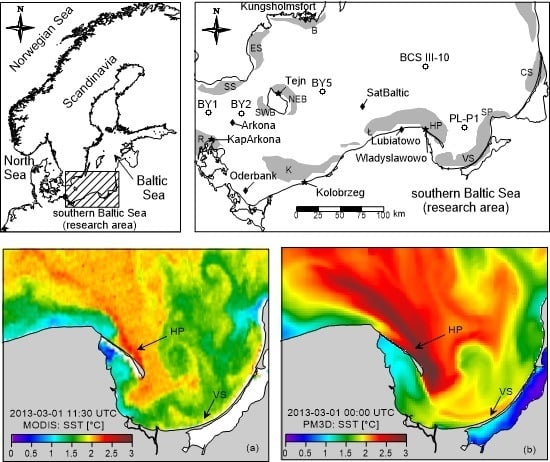
Figure 3.
Upwelling off the Hel Peninsula (HP) and off the Vistula Spit (VS): a comparison of SST distributions as determined from SST for 1 March 2013 in (a) the MODIS (Moderate-Resolution Imaging Spectroradiometer) image with (b) the simulation generated by the PM3D. White patches in the satellite image indicate cloud-covered areas.

Figure 4.
Water temperature fluctuations recorded by the SatBaltic buoy (T_OBS) and simulations produced by PM3D (T_PM3D) between 26 February and 3 March 2013.
Figure 4.
Water temperature fluctuations recorded by the SatBaltic buoy (T_OBS) and simulations produced by PM3D (T_PM3D) between 26 February and 3 March 2013.

Figure 5.
An upwelling off the Hel Peninsula (HP): a comparison of SST distributions as determined from SST for 28 February 2011 in (a) the AVHRR image with (b) the simulation generated by the PM3D. For explanation of white patches, see Figure 3.
Figure 5.
An upwelling off the Hel Peninsula (HP): a comparison of SST distributions as determined from SST for 28 February 2011 in (a) the AVHRR image with (b) the simulation generated by the PM3D. For explanation of white patches, see Figure 3.

Figure 6.
Upwelling off the Hel Peninsula (HP), off the Vistula Spit (VS) and off the Curonian Spit (CS): a comparison of SST distributions as determined from SST for 27 January 2012 in (a) the AVHRR image with (b) the simulation generated by the PM3D. The presence of upwelling off the Sambia Peninsula (SP) could not be classified unequivocally. For explanation of white patches, see Figure 3.

Figure 7.
Upwelling at the southern Baltic coast: a comparison of SST distributions as determined from SST for 30 January 2012 in (a) the AVHRR image with (b) the simulation generated by the PM3D, abbreviations as in Table 1. For explanation of white patches, see Figure 3.


Figure 8.
Upwelling off the islands of Rügen (R) and Bornholm (NEB): a comparison of SST distributions as determined from SST for 31 January 2012 in (a) the AVHRR image with (b) the simulation generated by the PM3D. For explanation of white patches, see Figure 3.
Figure 8.
Upwelling off the islands of Rügen (R) and Bornholm (NEB): a comparison of SST distributions as determined from SST for 31 January 2012 in (a) the AVHRR image with (b) the simulation generated by the PM3D. For explanation of white patches, see Figure 3.

Figure 9.
An upwelling off the Island of Rügen (R): a comparison of SST distributions as determined from SST for 4 January 2016 in (a) AVHRR and (b) MODIS satellite images with (c) the simulation generated by the PM3D. For explanation of white patches, see Figure 3.
Figure 9.
An upwelling off the Island of Rügen (R): a comparison of SST distributions as determined from SST for 4 January 2016 in (a) AVHRR and (b) MODIS satellite images with (c) the simulation generated by the PM3D. For explanation of white patches, see Figure 3.

Figure 10.
PM3D-generated sea surface temperature distribution on 23 February 2017 showing the presence of upwellings off southern Skåne (SS), off eastern Skåne (ES), and off Blekinge (B).
Figure 10.
PM3D-generated sea surface temperature distribution on 23 February 2017 showing the presence of upwellings off southern Skåne (SS), off eastern Skåne (ES), and off Blekinge (B).

Figure 11.
Upwelling at the Swedish coast: a comparison of SST distributions as determined from SST for 24 February 2017 in (a) the AVHRR image with (b) the simulation generated by the PM3D, abbreviations as in Table 1. For explanation of white patches, see Figure 3.


| No. | Abbreviation | Area |
|---|---|---|
| 1 | CS | off the Curonian Spit |
| 2 | SP | off the Sambia Peninsula |
| 3 | VS | off the Vistula Spit |
| 4 | HP | off the Hel Peninsula |
| 5 | Ł | Polish coast off Łeba |
| 6 | K | Polish coast off Kołobrzeg |
| 7 | R | off the Island of Rügen |
| 8 | SWB | off southwestern Bornholm |
| 9 | NEB | off northeastern Bornholm |
| 10 | SS | off southern Skåne |
| 11 | ES | off eastern Skåne |
| 12 | B | off Blekinge |
Table 2.
The number of available satellite sea surface temperature (SST) images in January and February (2010–2017).
Table 2.
The number of available satellite sea surface temperature (SST) images in January and February (2010–2017).
| Year | AVHRR | MODIS |
|---|---|---|
| 2010 | 46 | 19 |
| 2011 | 145 | 8 |
| 2012 | 112 | 12 |
| 2013 | 9 | 3 |
| 2014 | 50 | 14 |
| 2015 | 45 | 16 |
| 2016 | 139 | 20 |
| 2017 | 126 | 18 |
| Sum | 672 | 110 |
Table 3.
Statistical indicators of differences between the modelled and in situ measurements of SST in the southern Baltic Sea.
Table 3.
Statistical indicators of differences between the modelled and in situ measurements of SST in the southern Baltic Sea.
| Station | Bias [°C] | RMSE [°C] | Correlation Coefficient | Number of Records | Observation Period |
|---|---|---|---|---|---|
| Kołobrzeg | −0.51 | 1.33 | 0.973 | 30238 | 2014–2017 |
| Władysławowo | 0.00 | 1.44 | 0.969 | 30235 | 2014–2017 |
| Lubiatowo | −0.44 | 0.57 | 0.993 | 2080 | 2015–2017 |
| Oder Bank | −0.38 | 0.50 | 0.996 | 5885 | 2010–2017 |
| Arkona | −0.16 | 0.63 | 0.994 | 8384 | 2010–2017 |
| Kap Arkona | −0.52 | 1.17 | 0.978 | 29420 | 2010–2017 |
| Tejn | −0.23 | 0.93 | 0.987 | 66307 | 2010–2017 |
| Kungsholmsfort | −0.39 | 1.13 | 0.983 | 60165 | 2010–2017 |
| SatBałtic | −0.09 | 0.47 | 0.997 | 2336 | 2013 |
| PL-P1 | −0.18 | 0.69 | 0.994 | 111 | 2010–2017 |
| BCS III-10 | 0.04 | 0.68 | 0.995 | 97 | 2010–2015 |
| BY1 | 0.23 | 0.70 | 0.994 | 45 | 2010–2012 |
| BY2 | −0.11 | 0.73 | 0.992 | 143 | 2010–2015 |
| BY5 | 0.03 | 0.50 | 0.997 | 147 | 2010–2015 |
Table 4.
A comparison of simultaneous occurrence of upwelling event in model simulation (M) and observed in satellite images (S) in individual areas of the Baltic Sea (January and February 2010–2017).
Table 4.
A comparison of simultaneous occurrence of upwelling event in model simulation (M) and observed in satellite images (S) in individual areas of the Baltic Sea (January and February 2010–2017).
| Area | Number of Cases Analysed | M(+), S(+) | M(+), S(−) | M(−), S(+) | M(−), S(−) | Consistent Situations | Inconsistent Situations | ||||||||
|---|---|---|---|---|---|---|---|---|---|---|---|---|---|---|---|
| No. | % | No. | % | No. | % | No. | % | No. | % | No. | % | ||||
| CS | 81 | 12 | 14.8 | 2 | 2.5 | 0 | 0.0 | 67 | 82.7 | 79 | 97.5 | 2 | 2.5 | ||
| SP | 79 | 6 | 7.6 | 4 | 5.1 | 0 | 0.0 | 69 | 87.3 | 75 | 94.9 | 4 | 5.1 | ||
| VS | 90 | 16 | 17.8 | 11 | 12.2 | 9 | 10.0 | 54 | 60.0 | 70 | 77.8 | 20 | 22.2 | ||
| HP | 88 | 32 | 36.4 | 8 | 9.1 | 1 | 1.1 | 47 | 53.4 | 79 | 89.8 | 9 | 10.2 | ||
| Ł | 82 | 1 | 1.2 | 0 | 0.0 | 4 | 4.9 | 77 | 93.9 | 78 | 95.1 | 4 | 4.9 | ||
| K | 89 | 8 | 9.0 | 4 | 4.5 | 8 | 9.0 | 69 | 77.5 | 77 | 86.5 | 12 | 13.5 | ||
| R | 104 | 25 | 24.0 | 5 | 4.8 | 4 | 3.8 | 70 | 67.3 | 95 | 91.3 | 9 | 8.7 | ||
| SWB | 88 | 0 | 0.0 | 1 | 1.1 | 1 | 1.1 | 86 | 97.7 | 86 | 97.7 | 2 | 2.3 | ||
| NEB | 91 | 2 | 2.2 | 9 | 9.9 | 5 | 5.5 | 75 | 82.4 | 77 | 84.6 | 14 | 15.4 | ||
| SS | 102 | 1 | 1.0 | 0 | 0.0 | 1 | 1.0 | 100 | 98.0 | 101 | 99.0 | 1 | 1.0 | ||
| ES | 103 | 24 | 23.3 | 7 | 6.8 | 3 | 2.9 | 69 | 67.0 | 93 | 90.3 | 10 | 9.7 | ||
| B | 102 | 8 | 7.8 | 4 | 3.9 | 3 | 2.9 | 87 | 85.3 | 95 | 93.1 | 7 | 6.9 | ||
Note: M(+), S(+): both M and S showed the presence of an upwelling; M(+), S(−): M showed the presence of an upwelling, S − the absence of an upwelling; M(−), S(+): M showed the absence of an upwelling, S—the presence of an upwelling; M(−), S(−): both M and S showed the absence of an upwelling; situations where upwelling or its absence were observed in both image and model results were classified as consistent.
Table 5.
Upwelling events as recorded on satellite images and modelled by the Parallel Model 3D (PM3D).
Table 5.
Upwelling events as recorded on satellite images and modelled by the Parallel Model 3D (PM3D).
| Area | Satellite SST Images | PM3D | |||||
|---|---|---|---|---|---|---|---|
| Available Dates 1 | % | Upwelling Events | Available Dates | Upwelling Events | |||
| No. | % | No. | % | ||||
| CS | 81 | 17.1 | 12 | 14.8 | 466 | 52 | 11.2 |
| SP | 79 | 16.7 | 6 | 7.6 | 466 | 35 | 7.5 |
| VS | 90 | 19.0 | 25 | 27.8 | 466 | 137 | 29.4 |
| HP | 88 | 18.6 | 33 | 37.5 | 466 | 202 | 43.3 |
| Ł | 82 | 17.3 | 5 | 6.1 | 466 | 4 | 0.9 |
| K | 89 | 18.8 | 16 | 18.0 | 466 | 40 | 8.6 |
| R | 104 | 21.9 | 29 | 27.9 | 466 | 114 | 24.5 |
| SWB | 88 | 18.6 | 1 | 1.1 | 466 | 3 | 0.6 |
| NEB | 91 | 19.2 | 7 | 7.7 | 466 | 43 | 9.2 |
| SS | 102 | 21.5 | 2 | 2.0 | 466 | 2 | 0.4 |
| ES | 103 | 21.7 | 27 | 26.2 | 466 | 79 | 17.0 |
| B | 102 | 21.5 | 11 | 10.8 | 466 | 46 | 9.9 |
1 The availability of SST satellite images.
© 2019 by the authors. Licensee MDPI, Basel, Switzerland. This article is an open access article distributed under the terms and conditions of the Creative Commons Attribution (CC BY) license (http://creativecommons.org/licenses/by/4.0/).
Share and Cite
MDPI and ACS Style
Kowalewska-Kalkowska, H.; Kowalewski, M. Combining Satellite Imagery and Numerical Modelling to Study the Occurrence of Warm Upwellings in the Southern Baltic Sea in Winter. Remote Sens. 2019, 11, 2982. https://doi.org/10.3390/rs11242982
AMA Style
Kowalewska-Kalkowska H, Kowalewski M. Combining Satellite Imagery and Numerical Modelling to Study the Occurrence of Warm Upwellings in the Southern Baltic Sea in Winter. Remote Sensing. 2019; 11(24):2982. https://doi.org/10.3390/rs11242982
Chicago/Turabian StyleKowalewska-Kalkowska, Halina, and Marek Kowalewski. 2019. "Combining Satellite Imagery and Numerical Modelling to Study the Occurrence of Warm Upwellings in the Southern Baltic Sea in Winter" Remote Sensing 11, no. 24: 2982. https://doi.org/10.3390/rs11242982
Note that from the first issue of 2016, this journal uses article numbers instead of page numbers. See further details here.