Deriving the Reservoir Conditions for Better Water Resource Management Using Satellite-Based Earth Observations in the Lower Mekong River Basin


Department of Biological Systems Engineering, Virginia Polytechnic Institute and State University, Blacksburg, VA 24061, USA
*
Author to whom correspondence should be addressed.
Remote Sens. 2019, 11(23), 2872; https://doi.org/10.3390/rs11232872
Submission received: 17 October 2019
/
Revised: 26 November 2019
/
Accepted: 27 November 2019
/
Published: 3 December 2019
Abstract
:The Mekong River basin supported a large population and ecosystem with abundant water and nutrient supply. However, the impoundments in the river can substantially alter the flow downstream and its timing. Using limited observations, this study demonstrated an approach to derive dam characteristics, including storage and flow rate, from remote-sensing-based data. Global Reservoir and Lake Monitor (GRLM), River-Lake Hydrology (RLH), and ICESat-GLAS, which generated altimetry from Jason series and inundation areas from Landsat 8, were used to estimate the reservoir surface area and change in storage over time. The inflow simulated by the variable infiltration capacity (VIC) model from 2008 to 2016 and the reservoir storage change were used in the mass balance equation to calculate outflows for three dams in the basin. Estimated reservoir total storage closely resembled the observed data, with a Nash-Sutcliffe efficiency and coefficient of determination more than 0.90 and 0.95, respectively. An average decrease of 55% in outflows was estimated during the wet season and an increase of up to 94% in the dry season for the Lam Pao. The estimated decrease in outflows during the wet season was 70% and 60% for Sirindhorn and Ubol Ratana, respectively, along with a 36% increase in the dry season for Sirindhorn. Basin-wide demand for evapotranspiration, about 935 mm, implicitly matched with the annual water diversion from 1000 to 2300 million m3. From the storage–discharge rating curves, minimum storage was also evident in the monsoon season (June–July), and it reached the highest in November. This study demonstrated the utility of remote sensing products to assess the impacts of dams on flows in the Mekong River basin.
1. Introduction
Remote sensing data have been used in water resource studies to estimate rainfall, evapotranspiration (ET), soil moisture [1], runoff, floods, droughts, snow water equivalent [2], and irrigation [3]. Apart from providing crucial information at the global scale, remote sensing can also be used as a proxy to the observed data in data-scarce regions. The water resources’ spatial and temporal variations are not confined to country boundaries. Therefore, it requires a broader consensus approach covering social, environmental, technical, and economic aspects for efficient management [4]. The United Nations has identified water usage by different sectors as the basis for the complexities and the principle for the allocation of the international river waters [5]. Despite a few studies that used hydrological and hydraulic models to understand dam characteristics, it is difficult to develop plans for the operation and maintenance of reservoirs without any real monitoring and modeling [6,7,8,9,10].
Since the extent of water use is related to the availability of storage in reservoirs, estimating the change in storage over a seasonal or annual scale is critical. Moreover, reservoir storage estimation is dependent on many unknown factors, including diversion, inflow, and day-to-day operations. The complexities exacerbate for transboundary rivers because many stakeholders are involved across many countries. Cascading of dams in the main stem and tributaries as well as unmindful development within the catchment can further complicate conditions. Therefore, quantifying diversion from the reservoirs will be crucial to assess food and water security concerns of the agricultural regions.
Advances in remote sensing techniques can potentially aid in estimating crop water requirements or diversion for irrigation using the storage change estimations and inflow and outflow simulations from the hydrological model. However, accurate estimates of storage and diversion require a well-calibrated hydrological model reflecting the basin in changing conditions [11]. Concisely, with the use of remote sensing data and good hydrological model, storage, inflow, and outflow can be estimated for the quantification of water diversion from reservoirs.
The Mekong River basin (MRB) is one of the largest transboundary basins in the world, shared by China, Myanmar, Thailand, Lao PDR, Cambodia, and Vietnam. The livelihood of more than sixty million people in the Lower Mekong Basin (LMB) is dependent on the Mekong River for agricultural activities—cultivation of rice, vegetables, livestock, fruit and nuts, and fisheries [12,13]. The intensity and highly predictable occurrence time of the peak are the defining characteristics of the large tropical monsoonal river [14], leading to a twentyfold increase in discharge between August and September. The MRB has high hydropower potential (~53,000 MW in the main stem and 35,000 MW from tributaries) [15] and is equipped with approximately 42 dams to harness the hydropower production [16]. There are plans to build 16 main stem and 110 tributary dams by 2030 [17,18]. The underdeveloped condition of the MRB in terms of river impoundments [19] and the sensitivity of the dam operation information are the fundamental cause of the lack of archived data sets in the region [20,21,22,23]. Most of the studies are performed through hydrological models, with remote sensing data merely used as forcing inputs for simulations [8,24,25].
Remote sensing plays a major role in characterizing the water bodies in remote areas where accessibility is an issue. The water level of the reservoir can be determined using the spatial extent estimated by the optical (Landsat 5 TM, Landsat 7 ETM+SLC-Off, Landsat 8 OLI-TIRS, and ASTER images) and synthetic aperture radar images (Cosmo SkyMed and TerraSAR-X) [26,27]. A combination of remote sensing satellite data products such as moderate resolution imaging spectroradiometer (MODIS) and altimeters can be used for the global monitoring of large reservoirs using unsupervised classification approach [28]. Similarly, variations in volumes of Lake Nasser and Toshka were estimated using the Landsat images and radar altimetry from TOPEX/Poseidon, Jason 1 and 2, Geostat, and Envisat [29]. The Landsat images were also helpful in the estimation of storages in small reservoirs in the Preto River Basin, Brazil [30]. Remote sensing was effective in estimating the reservoir volume located in the high topographic relief area in the Himalayan region in India [31]. In addition to monitoring the volume variation, remote sensing aids in establishing guidelines for reservoir operations. The rule curve of the Fengman reservoir (China) was derived using the normalized difference water index (NDWI) from the Landsat data [32]. The satellite imageries and water level data set from four different satellite altimetry databases—Global Reservoir and Lake Monitor (GRLM), River-Lake Hydrology (RLH), Hydroweb, and ICESat-GLAS level 2 global land surface altimetry data (ICESat-GLAS)—are available to estimate the water volume changes in lake and reservoirs [33,34,35]. Bonnema and Hossain [36] have used satellite observations to explore the artificial reservoirs’ operating pattern in the LMB—with two parameters affecting streamflow, residence time and flow alteration—and reported the range between 0.09 and 4.04 years and 11% and 130% of its natural variability, respectively. The satellite-based approach to assess the dam operation has been mainly confined to the United States, European, and African reservoirs.
Water diversion from the reservoirs for agriculture, domestic, and industrial purposes is also not explicitly inferred from these studies. Although the total annual runoff from the MRB is projected to increase by 21% by 2030 during the dry season and significantly during the wet season, the flow impoundment due to existing and planned dams is expected to affect the quantity and time of water availability to downstream regions [37,38]. However, water partitioning between different sectors (hydropower, irrigation, domestic, industrial, navigation, and environmental) is ambiguous since there is no clear idea of demand versus availability for a given season considering the dynamics of changes in land use, basin development, and climate. Alternatively, empirical relationships can be useful to represent the dynamics of the area, water depth, and discharge at each of the reservoir locations.
Considering the global applicability of remote sensing data sets, it is ideal for any methodology to be scalable to other locations so that a standard procedure can be developed to assess water management of multipurpose reservoirs. This will help assess the need for robust observational data for water levels from a range of reservoirs to scale (repeat cycle or space/time resolution). Water diversion for irrigation, domestic, and industrial purposes will also enhance because of a large number of dams and will alter downstream flows. Therefore, it is important to assess the dams’ cumulative impacts as it can directly alter the flows, storage, and diversions.
To meet the increasing water demand due to the growing population, the amount of water required is also expected to increase for food grain production. The nexus among food, energy, and water is also evident from the large water diversion for irrigation purposes, which may potentially hamper hydropower generation as the reservoir waterhead that governs the efficiency of electricity production. Therefore, the proposed approach in this study can help in the sustainable management of the reservoirs in the context of food-energy-water nexus. Specifically, once the understanding of water resources in the basin is established, it can help divide the resources between diversion and storage, which in turn provides the guidelines for hydropower production and river basin management.
The objectives of this study were to (a) develop a methodology to estimate dam characteristics such as storage variation, inflow, and outflow from the reservoirs using remotely sensed observations; (b) analyze the effect of dams on the downstream region through estimating change in the flow and diversion from the reservoirs; and (c) characterize dam operation patterns defined by the rule curves. To investigate these scientific tasks, we utilized remote sensing products to compute storage variation in the reservoirs by combining the simulated inflows from the hydrological model to quantify the outflow from the dams and by developing rule curves based on the total reservoir storage. Furthermore, water diversions from the reservoirs were estimated using ET from MODIS as a proxy to crop water demand. The altimetry data set from GRLM and Hydroweb databases and the satellite imagery from Landsat 8 and Sentinel-2 and the variable infiltration capacity (VIC) model were collectively employed, in addition to the observed reservoir data for the dams, where available, in the basin.
2. Materials and Methods
2.1. Study Area
The Mekong River originates in Qinghai Province, China, and flows 4800 km to reach the South China Sea by forming the Mekong delta near the mouth of the river and draining an area of nearly 765,000 km2. The MRB is associated with high annual mean flows of approximately 15,000 km3/year. The precipitation in the region is defined by the monsoon season (June–November), during which the basin receives the majority of the rainfall. The spatial variability of precipitation is high, with the mean annual rainfall of 3000 mm in the uplands in the Lao PDR and Cambodia and 1000 to 1600 mm in northeastern Thailand. The temperatures during the warmest months (March and April) fluctuate between 30 °C and 38 °C and in the winter around 15 °C. The large river flow combined with an elevation gradient of 4000 m makes the MRB the ideal basin for hydropower development.
The extensive waterlogging and inundation during the wet season support irrigated wet-season rice as the primary crop in the MRB. The Mekong river also reinforces the global fish market through an annual fish catch of more than 4.4 million tons. Hence, sustainable livelihood in the MRB is dependent on the dams’ efficient operation and the management of the unknown consequences of presently commissioned dams on the river flow. Three dams with a total reservoir storage capacity of more than 1900 million m3 and a maximum reservoir area of greater than 200 km2 were selected for the analysis (Table 1 and Figure 1).
2.2. Data
2.2.1. Storage Estimation Based on Remote Sensing Data
The surface area of the reservoirs was estimated using the Landsat8 and Sentinel-2 reflectance images from 2013 to 2018 using the Remote Pixel tool [39] available online. The Landsat8 mission started in February 2013. There are a total of 11 bands capturing the spectral details with the green and near-infrared portion of the electromagnetic spectrum in band 3 and band 5, respectively. The product has a spatial resolution of 30 m for green and NIR bands and a temporal resolution of 16 days. Sentinel-2 images were employed to replace Landsat8 images with widespread cloud cover. Sentinel-2a and Sentinel-2b began in June 2015 and March 2017, respectively. The images from Sentinel-2 have 13 spectral bands with green and near-infrared portion of the electromagnetic spectrum in band 3 and band 8, respectively. The satellite imageries are available at 5-day temporal and 10 m spatial resolution for green and NIR bands. Landsat 8 and sentinel-2 images are available at the official US Geological Survey (USGS) website (https://earthexplorer.usgs.gov/).
The altimetry data sets have been used to extract the time series of water level in the reservoirs from 2013 to 2018. We used the altimetry data for some of the reservoirs in the MRB archived in the Hydroweb and GRLM from different satellites at a temporal resolution of 10 days. Additional details about the altimetry water level databases are available from Duan and Bastiannssen [34]. Hydroweb is created by LEOS/GOHS (Laboratoire d'études en géophysique et océanographie spatiales/Géophysique, Océanographie et Hydrologie Spatiales), using the altimetry data from ERS-1 (1991–1996), TOPEX/Poseidon (T/P; 1992–2006), ERS-2 (1995–2011), GFO (2000–present), Jason-1 (2001–2013), Envisat (2002–2012), Jason-2 (2008–present), and SARAL/AltiKa (2013–present). Cretaux et al. [40] describe the procedure for obtaining the water level in Hydroweb. The GRLM is developed by the United States Department of Agriculture’s Foreign Agricultural Service [41]. The database uses the altimetry data from TOPEX/Poseidon (1992–2006), Jason-1 (2001–2013), Envisat (2002–2012), and Jason-2 (2008–present) to derive the 10-day time series of reservoir water levels. Launched in 1992 as a joint mission of the American and French Space agencies, T/P provided the great advancement for radar altimetry research in the 20th century. Whilst most of these satellites are still operational and expected to continue functioning for the certain future period, the data from the new missions over the next few years (HaiYang-2, AltiKa, Sentinel-3, and Surface Water and Ocean Topography (SWOT)) will enable the water level monitoring at high temporal frequency [29].
The validation of the simulated storage was done using the daily time series of the observed reservoir storage in Thailand available from the Royal Irrigation Department between 2008 and 2018.
2.2.2. Reservoir Flow Estimation Based on Hydrological Modeling
The fluxes—such as ET, surface runoff, baseflow, snow water equivalent, and soil moisture—were simulated by the VIC model from the forcing variables, including daily precipitation, temperature (maximum and minimum), and wind speed at 0.25° spatial resolution for the LMB. The data between 1986 and 2016 were obtained from the gridded Global Meteorological Forcing Dataset (GMFD) [42]. The GMFD data set was also used to characterize future droughts and as the meteorological forcing for the VIC model in the LMB to study the effect of agricultural irrigation water abstraction [24,43].
Monthly estimates of ET were obtained using an 8-day composite MODIS product produced at 500 m resolution (MOD16A2 version 6) from 2008 to 2016. The MOD16A ET product represented the sum of transpiration by vegetation and evaporation from the canopy and soil surfaces. The estimation of MOD16 ET was carried out by the Numerical Terradynamic Simulation Group of the University of Montana using the improved ET algorithm by Mu et al. [44].
2.3. Approach
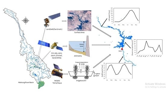
The methodology adopted in this work could be primarily classified into three major approaches: (a) estimation of reservoir total storage by regression analysis (Section 2.3.1), (b) estimation of reservoir inflows using the VIC model, and (c) calculation of outflows from the reservoirs using the water balance equation (Section 2.3.2). The schematic of the methodology is provided in Figure 2.
2.3.1. Storage Estimation Based on Remote Sensing Data
Estimates of variations in reservoir storages were derived by separating the total storage (S) into a variable component that fluctuated with the water level (i.e., live storage (Slive)) and the minimum fixed amount of water available throughout the period (i.e., dead storage (Sdead)).
Surface area variation (A): the extent (surface area) of the reservoirs was extracted by estimating the normalized difference water index (NDWI) [45] using the reflectance images described in Section 2.2.1. The region of interest (ROI) was carefully chosen based on a wet season Landsat image ensuring the size of ROI larger than the maximum surface area of each reservoir to minimize the vegetation influence on the NDWI calculation. The pixels with the positive NDWI value were classified as water pixels and the pixels with negative NDWI values were assumed to not accommodate surface water [46]. The number of identified water pixels was multiplied by the area of a single pixel, based on the spatial resolution of the image, for the accurate extraction and estimation of the surface area. The procedure was employed while processing the images to obtain the surface area (A) at 16-day intervals for the period between 2013 and 2018 (Figure 2a).
Water level variation (h): Satellite radar altimetry is an important technique primarily to measure water levels over the open ocean from space [47]. The factors constraining the application of the current satellite sensors in monitoring small water bodies include narrow swath, low spatial resolution, small footprint size, and complex terrain surrounding water bodies [28]. The processing of the raw data from the satellite requires a complex sequence of steps necessary for extracting usable water level information. Primarily, the objective of the procedure is to remove unwanted effects caused by the instrument, atmosphere, and ocean. The water level derivation from the satellite altimeters is based on the principle presented in Fu and Cazenave [47]. The surface height (h) with reference to an ellipsoid is based on arithmetic sum of satellite altitude (A), range between the satellite and the surface (R), and corrections (C). The local undulation of the geoid is reduced from surface height for estimation of physical height from the ellipsoidal height [48]. The reference of water for Hydroweb is the GRACE Gravity Model 02 geoid, while the GRLM has a mean 9-year T/P water level as a reference. Reservoir water levels were extracted from the altimetry data set as described in the earlier section. The altimetry data is with reference to the reference ellipsoid, which was converted into orthometric height by removing geoid height. The geoid approximately coincides with the mean sea level in the absence of all forces except gravity and centrifugal forces. As the altimetry data is with respect to reference geoid, the water level has positive and negative values (Figure 2b). However, the conversion factor between the satellite reference geoid and mean sea level was provided with the data set, but the relative values with respect to reference geoid were used in this analysis as live storage was governed by the change in the water level. Hence, in order to make calculations, the zero water level was considered as the reference datum. Since the altimetry information was available for a longer period from 2008 to 2018, with higher frequency and minimal nonusable data, this data set was more consistent than satellite imageries.
Regression analysis: Since the data set was derived from different satellites, a subset was selected for the regression analysis based on the coinciding date of acquisition of surface area images and the corresponding altimetry data. In order to avoid the deficiency of data for regression, the threshold of ±2 days of satellite pass date between these two sources was adopted. The selected altimetry data were assumed to reflect live storage variations; therefore, the minimum value of the selected altimetry data (hmin) corresponded to the null live storage (Slive = 0). Hence, the hmin was subtracted from the altimetry data to have the range of Slive initializing from zero. Mathematically, when h − hmin = 0, Slive = 0. The regression analysis was carried out to fit the surface area A and h − hmin values using a binomial function (Figure 2c). The coefficient of determination (R2) was used as the performance metric to infer the goodness of fit. Here, the nonzero surface area—when h − hmin and Slive are zero—suggested that the surface area was corresponding to the dead storage (Sdead).
Estimation of live storage (Slive) and total storage (S): The regression analysis yielded the relationship between A and h − hmin in the form of a binomial function, which can be expressed as:
where a, b, and c were the coefficients determined by the regression analysis. The expression for the Slive was derived in terms of water level by integrating Equation (1):
where a, b, and c were the same as Equation (1). The value of d was calculated by considering the condition that Slive = 0 when h − hmin = 0, resulting in the value of d = 0. The total storage of the reservoir was also the sum of live storage and dead storage. Mathematically, it can be expressed as:
Validation: The total storage estimation was entirely dependent on the altimetry data (Equation (3)) and was calculated for the same period as that of the altimetry data set. The simulated total storage of the reservoirs was compared with the observed storage variation to evaluate the performance of the approach (Figure 2d).
2.3.2. Reservoir Flow Estimation Based on Hydrological Modeling
Variable infiltration capacity model: The VIC is a semidistributed, physically based hydrological model that simulates fluxes by solving water and energy balance at the daily time step for each grid (here, 0.25° spatial resolution) separately, developed by Liang et al. [49]. The forcing parameters include meteorological data sets (i.e., daily precipitation, minimum and maximum temperature, and wind speed), along with vegetation parameters (i.e., land cover type, leaf area index (LAI), albedo, and soil parameters, such as field capacity and wilting point). Advanced very high-resolution radiometer (AVHRR) data at 1 km spatial resolution were used to develop vegetation type. Soil parameters were extracted from the Harmonized World Soil Database (HWSD) with the application of pedo-transfer functions of Cosby et al. [50] and soil class from the United States Department of Agriculture (USDA) classification. The Terrestrial Hydrology Research Group at Princeton University developed the meteorological forcing while the remaining forcing is available at the global scale from the VIC website. The model includes the Arno model formulation [51] for flow, the Penman-Monteith approach [52] for ET, and variable infiltration curve [53] for infiltration calculation. The VIC model provides only the fluxes for each grid at a daily time step based on the forcing parameters; therefore, to extract the accumulated effect at the particular location, a separate routing scheme developed by Lohmann et al. [54,55] was employed. The VIC model has been used by various studies for hydrological assessment [36,56,57,58,59,60,61]. The routing scheme explicitly routes the surface and subsurface flow within a grid using a unit hydrograph that contributes to a channel network where the node of the channel network represents each grid cell of the VIC model and linearized Saint-Venant equation [62,63]. The simulated flow was compared with the observed monthly discharge data from the seven gauging stations distributed across the basin, namely, Chiang Saen, Luang Prabang, Nakhon Phanom, Vientiane, Mukdahan, Pakse, and Kratie.
Estimation of outflow from reservoirs: Estimates of runoff simulated by the VIC model for the catchment area upstream of the dams were routed to the reservoirs for the estimation of inflow to the dams. Monthly outflows from the dams were then computed from the water balance equation for the reservoir accounting for the change in the reservoir storage and inflow to the dams, assuming negligible groundwater interactions:
where Qout was the monthly outflow from the dam in m3/s, Qin was the monthly inflow to the reservoir in m3/s, ΔS/Δt was the change in the storage volume with time in m3/s, A was the area of the reservoir’s water surface in m2, and P and E were the precipitation and open evaporation in m/s, respectively. The Qin and E on the reservoir were obtained from the simulation of the VIC model, whereas A was derived from the Landsat8 and Sentinel-2 imageries, and P was derived from GMFD. The change in the storage of the reservoir (∆S) was computed as the difference between the storage for the month in consideration and the previous month. The Qout from the dams simulated from Equation (4) was then validated against the observed flow from 2008 to 2016.
Estimation of rule curve: A rule curve is a plot between storage and time acting as a guideline for the reservoir operation and enabling to examine the efficiency in satisfying water demand by different sectors, namely, domestic, irrigation, industrial, hydropower, and ecosystem [64]. The rule curve was estimated using the monthly storage variation of the reservoirs derived using satellite images and altimetry data from 2008 to 2016. The average rule curve was derived by calculating the mean value of the storage variation for each month from 2008 to 2016. While the minimum and maximum values for each month define the lower and upper rule curve, respectively. The lower rule curve governs the water volume maintenance to avoid the risk of water shortage during the dry season, on the other hand, the upper rule curve guides the risk aversion of floods.
3. Results
3.1. Storage Estimation Based on Remote Sensing Data
Figure A1 shows the water mask of the Lam Pao, Sirindhorn, and Ubol Ratana reservoirs extracted from the Landsat8 and Sentinel-2 satellite imageries demonstrating the surface area’s seasonal expansion and contraction. The surface area of the Lam Pao reservoir ranged between 80 km2 and 236 km2 from 2013 to early 2018 (Figure 3a). The reservoir’s water depth from 2008 to 2018 was similar to that of surface area and correlated well (Figure 3b). The Lam Pao reservoir experienced a gradual increase in the surface area from 2015 to 2017 due to the increase in the annual precipitation in the catchment area.
The surface area of the Sirindhorn reservoir varied from 206 to 285 km2 between 2013 and 2017 (Figure 3g). The gradual increase in the Sirindhorn reservoir’s surface area from 2015 to 2017 was similar to that of Lam Pao. The Ubol Ratana reservoir’s surface area was the highest with 370 km2 in November 2017 and the lowest with 120 km2 in May 2016. The variations between the maximum and minimum surface area of the reservoirs accounted for 64%, 27%, and 58% of the maximum reservoir areas for Lam Pao, Sirindhorn, and Ubol Ratana, respectively. Deficiency of the data for Ubol Ratana in the GRLM and the Hydroweb databases restricted the computation of reservoir depths and total storage. However, the observed total storage of the Ubol Ratana from 2008 to 2018 was used for further analysis. The reservoirs’ water depth variation inferred from the altimetry data set was more consistent than the surface area, thus providing the information at high frequencies (Figure 3).
More than 45 pairs of surface area and water level for Lam Pao and Sirindhorn were selected for the regression analysis to estimate the Slive and S (Figure 3). The relationships between the area and depth expressed as quadratic equations were shown in Figure 3c,i with an R2 value greater than 0.90. The depth-area equations were used to derive volume-depth relationships (Equations (5) and (6)). The live storages for these reservoirs were estimated from the water levels available from GRLM and Hydroweb data sets and using the cubic equations of volume-depth relationships (Equations (7) and (8))
Water level anomalies from the altimetry data set were used to estimate reservoir total storage (total storage = live storage + dead storage) at a 10-day interval from 2008 to 2018. The time series of the simulated total storage variation of the Lam Pao and Sirindhorn reservoirs were validated by comparison with the observed storage from the reservoir database (Figure 3). The total storage of the Lam Pao reservoir varied from 245 to 1790 million m3, accounting for the dead storage as 245 million m3 (Figure 3d). The simulated total storage of the reservoir agreed well with the observed storage with the Nash–Sutcliffe efficiency coefficient (NSE) [65] and R2 values greater than 0.9. The ensemble mean was used to estimate the monthly variations in total storage for the Lam Pao reservoir (Figure 3e). The lowest volume in the reservoir was observed during May (450 million m3), which could be a measure adopted to allow the accumulation of inflows during the monsoon period that resulted in the highest volume during October (1170 million m3); and generally, it was available for release till the onset of the next monsoon season.
For the Sirindhorn reservoir, the NSE and R2 values between the observed and simulated total storage were estimated as 0.98 and 0.99, respectively (Figure 3j). Estimates of monthly variations in total storage showed higher predictability of volume-depth aided by area-depth relationships and a lesser fluctuation in the surface area. The fluctuation in the observed total storage of the Ubol Ratana reservoir from 2008 to 2018 ranged between 500 and 2800 million m3; however, the average total storage was 990 million m3 from 2013 to 2015 (Figure 3n). The reservoirs’ annual maximum total storage was in close agreement with the annual precipitation over the catchment, and the storage variation range was dependent on the catchment area’s size. Simulation of reservoir total storage was substantially better with higher R2 (>0.9) values between observed and simulated storage for Lam Pao and Sirindhorn reservoirs (Figure 3f,l).
3.2. Reservoir Flow Estimation Based on Hydrological Modeling
3.2.1. Simulated Streamflow
The VIC model was used to simulate monthly inflows to the reservoirs from 2008 to 2016. Previously, the VIC model’s calibration and evaluation were performed using the monthly discharge data from the gauging stations. The observed monthly discharge data were acquired from the MRC hydrometeorological database [66]. The VIC model’s performance in simulating the streamflow improved substantially with the calibration of parameters such as variable infiltration curve parameter (bi), depth of the second and third soil layers (D), fraction of maximum velocity of baseflow where nonlinear baseflow began (Ds), and fraction of maximum soil moisture where nonlinear baseflow occurred (Ws), with the allowable range being 0.1–0.5, 0.1–1.5, 0–0.4, and 0.5–1.0, respectively.
The VIC model precisely simulated the observed streamflow with an NSE value of more than 0.85 and an R2 value of more than 0.90 during the calibration period (Table A1 and Figure A2). For the evaluation period, the NSE value remained greater than 0.85 except for Luang Prabang (NSE = 0.80), while the R2 value was over 0.88
The comparisons of observed and simulated inflows to the dams were necessary to evaluate the VIC model’s performance for the tributary of the Mekong River. The monthly inflows to the dams were compared from 2008 to 2016 for Lam Pao and Ubol Ratana and 2009–2016 for Sirindhorn. The NSE values between the observed and simulated inflows were estimated as 0.77, 0.64, and 0.65 for Lam Pao, Sirindhorn, and Ubol Ratana dams, respectively, whereas the R2 values were greater than 0.67 (Figure 4, Table A2)
3.2.2. Effect of Dams on Outflows
Simulated inflows and storage change were used to estimate the monthly outflows from the reservoirs as shown in Equation (4). The estimation period of the outflow from the dams remained the same as the inflow period except for Lam Pao, where the computation of total storage variation started from 2009. Simulated outflows were validated with observed flows by computing NSE and R2 values (Figure 4, Table A2). The NSE values improved at Sirindhorn and Ubol Ratana with values up to 0.65 and 0.67, respectively. However, the NSE value for the Lam Pao Dam remained the same as the inflow because of marginally lower NSE value between observed and simulated total storage than other reservoirs, but the improvement was evidenced in the coefficient of determination (R2 = 0.85).
While the characteristics of the monthly outflows and inflows were similar, the reduction in the magnitude of outflows due to impoundments was noticeable. The peak flow occurred during 2010–2011 for Lam Pao and Ubol Ratana, while Sirindhorn’s observed peak flows occurred in 2011 and 2013–2014. High precipitation during the peak flow period was the primary cause of high inflows and the resulting outflows in the reservoirs. The common peak flow period for the Lam Pao and Ubol Ratana was due to their adjacent catchment area. Although the anomaly of the monthly inflow and outflow remained similar, the seasonal variation of the flows exhibited contrasting characteristics during the wet (June–November) and dry (December–May) periods within a year (Figure 4). During the wet period, the basin received a major proportion (79%) of the annual precipitation, resulting in large inflows to the dams (Figure 4c,f,i). The total storage of the reservoirs was also at a minimum level before the onset of the monsoon (May–June; Figure 3), allowing the monsoon flows to be accumulated into the reservoirs. As a result, the outflows from the dams were less than the inflows during the wet period, and it would be safe to assume that some of the wet season release could be meant for the minimum ecological flow requirements. On the other hand, the inflows to the reservoirs were negligible during the dry period because of decreased precipitation. However, the expected demands for domestic, industrial, and energy generation purposes must be met during this period, and the reservoir release was higher. The higher outflows during the dry period also enabled the retention of increased flows from monsoonal rain events in the following season.
Figure 5 and Table 1 show the percentage change in outflows from the dams with respect to inflows during the wet (blue) and the dry (red) periods from 2008 to 2016 for Lam Pao, Sirindhorn, and Ubol Ratana. Each year was segregated into two periods: wet season (June–November) and dry season (December–May). Based on the storage variation (Figure 3e,k,o), the wet season (June–November) shows the consistent increase in the reservoir volume, hence during this period of the year, the reservoir was storing water. On the other hand, during the dry season (December–May), the volume of the reservoir decreased, hence the reservoir was augmenting inflow. The average increase in the outflow during the dry period was estimated as 94% with respect to the inflow for the Lam Pao reservoir, but the outflow decreased by 55% during the wet period. However, the average outflow magnitudes between the dry and wet periods remained almost equal, with a monthly discharge of 42 m3/s and 47 m3/s, respectively. Management of reservoirs between seasons affects flow maintenance despite natural and anthropogenic-induced changes to the climate and monsoon rains. The changes in the outflow from the Lam Pao reservoir were always negative relative to inflows for the wet period except during 2012. The annual precipitation during 2012 (31% less than the historical average) was the lowest for the period of analysis, generating low inflow to the Lam Pao from the small catchment, but the average outflow was maintained throughout the year, causing an increase of 29% in the outflows relative to the inflows during the wet period. The outflow also remained equal to the inflow during the dry period (1.4% increase in outflow). Storage from these reservoirs during the low-precipitation year enabled flows to be maintained from the preceding high-precipitation year (2011), but the effect was reflected with decreased storage in the reservoir during 2012–2013.
For the Sirindhorn Dam, the average outflow from the reservoirs varied from −70% during the wet period to +36% during the dry period, with an average outflow of 40 m3/s and 25 m3/s during the wet and dry periods, respectively (Figure 5c). The change in the flow during the dry period was governed by the annual precipitation, evident during the high-precipitation years of 2009, 2011, and 2014 (Figure 5d), while the outflow change remained negative for the rest of the years. For Ubol Ratana Dam, the outflow from the reservoir varied from −23% to +93%, with an average value of 60% during the wet season from 2008 to 2016. However, the change in flows during the dry season increased up to 54% from 2008 to 2011 and then gradually decreased up to 44% in the remaining period (Figure 5e). The average outflow from the reservoir was estimated as 54 m3/s, which remained the same throughout the year, but the considerable fluctuation in the inflow—especially during 2010, 2011, and 2013—enhanced the flow difference between inflow and outflow from the reservoir. The total storage in the Ubol Ratana reservoir diminished during 2012–2016, with average storage of 990 million m3. Fluctuation in the annual precipitation and the large size of the catchment area of the Ubol Ratana reservoir minimized the variability imposed by climate and anthropogenic factors.
3.3. Rule Curve
Figure 6a–c showed the rule curve for Lam Pao, Sirindhorn, and Ubol Ratana reservoirs, respectively, derived from the monthly total storage between 2008 and 2016. The average storage of the Lam Pao varied from 410 million m3 to 1025 million m3 with a mean value of 720 million m3 (Figure 6a). For Sirindhorn, the minimum and maximum values of the reservoir storage were estimated as 850 million m3 and 1630 million m3, respectively, and the mean value was observed as 1250 million m3. A wide range in the total storage of the reservoir was noticeable for Ubol Ratana from 720 to 1750 million m3, constituting the mean storage of 1150 million m3.
Storage estimates showing seasonal differences were similar for all the reservoirs, with increasing magnitude from May to October resulting from lower outflow than inflow. On the contrary, there was decreasing storage from November to April as discharges were regulated with higher outflows. Furthermore, the change in the variation of the reservoirs’ storage was negative for May–October and positive for November–April with respect to the mean annual storage. The total storage declined up to 43%, 32%, and 38% below the mean annual storage for Lam Pao, Sirindhorn, and Ubol Ratana, respectively; however, the average declines during May–October were estimated as 28%, 21%, and 28%. On the other hand, the highest increases in storage were computed as 43%, 30%, and 51% above the mean storage for Lam Pao, Sirindhorn, and Ubol Ratana, respectively. The spread range between the upper and lower limits of the rule curve varied from 300 to 970 million m3 for Lam Pao, whereas the values were 71–860 million m3 and 350–2100 million m3 for Sirindhorn and Ubol Ratana, respectively. Figure 6d,e showed the relationship between the storage and water level of the Lam Pao and Sirindhorn reservoirs. The rule curve of the Lam Pao and Sirindhorn can be transformed into the water level variation using the quadratic Equations (9) and (10), respectively, with an R2 value greater than 0.99:
where storage is the reservoir’s total storage in million m3 defining the rule curve, and depth is the reservoir’s water level in meters.
3.4. Water Diversion from the Reservoirs and ET Analogy
The comparison of the seasonal variation of inflows and outflows from the reservoirs showed higher outflows during the dry season relative to inflows. However, the difference between the inflow and outflow from the reservoir was greater during the wet season, which resulted in the increased impoundment. Even the outflow was less than the inflow for the reservoirs during the dry period (i.e., 2016 in Lam Pao, 2015–2016 in Sirindhorn, and 2014–2016 in Ubol Ratana). As a result, the reservoir’s total storage volume further increased during the period of inflow, exceeding outflow in the dry season. Despite these dynamic interseasonal and interannual changes, the reservoirs’ storage variation showed no response to any particular situation, even when the storage volume in the Ubol Ratana reservoir declined during 2013–2016. Figure 4c,f,i shows the difference between the inflow volume and outflow volume does not remain the same for the wet and dry season. In other words, the water stored in the reservoir during the wet season was more than the water released during the dry season. As a result, the volume of the storage should increase every year with the assumption that there is no other water loss. However, Figure 3 shows that the average reservoir volume remained the same for Lam Pao and Sirindhorn, moreover the volume decreased for Ubol Ratana during 2012–2016. Figure 7 showed the annual and monthly variation of the excess water that remained unaccounted in the flow estimation from the Lam Pao, Sirindhorn, and Ubol Ratana Dams between 2008 and 2016.
The mean annual diversions from Lam Pao (600 million m3), Sirindhorn (1380 million m3), and Ubol Ratana (1560 million m3) were proportional to the total storage capacity of the reservoirs. The monthly variation of the diversion from the reservoir was similar to the ET (Figure 7). The approach is capable of handling storage based on the purpose of each reservoir under consideration (for example flood control, irrigation, or hydropower as a unique purpose). If there is a multi-use purpose reservoir that exists, the rule curve should be based on historic handling of storage for different use (domestic, irrigation, industrial, hydropower, etc.). In this study, to determine the cause of the water diversion, the comparison was made with ET, as ET is directly proportional to the net irrigation water requirement (NIWR) according to Food and Agriculture Organization (FAO). However, it was just the assumption that the water is diverted for irrigation purposes. Monthly ET, using MODIS ET, estimates were the lowest during January–March, which increased gradually between May and October; afterward, the ET decreased during the last two months of the year. The variations in ET were in good agreement with the crop-growing periods for the Thailand region. The sowing and growing period of the main rice crop occurred from May to September, followed by harvesting. Therefore, the ET was the highest during May to October with an estimation of 88 mm/month, 100 mm/month, and 107 mm/month for Lam Pao, Sirindhorn, and Ubol Ratana, respectively. The second crop of rice or maize or sorghum was also grown over the year. The monthly water assessment in diversion and ET (Figure 7b,d,f) showed similar patterns during January–April, and November–December. However, water diversion was suppressed compared to ET from May to October. Although the availability of water during the monsoon season was not limited, the demand was still high but diminished slightly because of monsoonal rains, which resulted in gradual reductions in the diversion.
4. Discussion
The satellite imageries show seasonal expansion and contraction of the surface area of the Lam Pao, Sirindhorn, and Ubol Ratana reservoirs (Figure A1). The surface area’s fluctuation followed the monsoon season, resulting in shrinkage during the premonsoon season (May) and swelling at the end of the season (November). The lesser variation in the surface area of the Sirindhorn (79 km2), as compared with Lam Pao (154 km2), was due to dam’s smaller catchment area. The minimum surface area remained constant possibly due to the management of the reservoir. The large variation in the surface area was caused by the high flows contributed by the large catchment area of the Ubol Ratana dam. The reservoirs’ maximum surface areas simulated by the satellite imageries were 239.6 km2, 283.6 km2, and 369.2 km2 for Lam Pao, Sirindhorn, and Ubol Ratana, respectively, with a difference of 0.17%, 1.55%, and 11.05% as compared with the observed surface area.
The results obtained using the remote sensing data were in agreement with the published literature. The simulated reservoir storage closely represents the observed storage with 15.73% relative root mean square error (RRMSE, R2 = 0.82) for Lam Pao and 3.65% RRMSE (R2 = 0.98) for Sirindhorn. A similar approach was adopted by Bonnema and Hossain [36] for the storage estimation of reservoirs. However, Bonnema and Hossain [36] used LandSat8 for the estimation of surface area, while this study uses Sentinel2 along with the LansSat8 images. The altimeter data was also used for the water level extraction in this study in contrast to the trapezoidal approximation using the Shuttle Radar and Topography Mission (SRTM) and the digital elevation map (DEM) to calculate total storage variation of the reservoirs. Landsat 8 images derived NDWI were used for the surface area calculation, while the water level was obtained from Shuttle Radar Topography Mission digital elevation model (SRTM DEM) and Jason-2 satellite altimetry mission for Sirindhorn and Oroville reservoir, respectively. Comparison of the simulated and observed storage volume agreed to within 20% of RRMSE. NDWI was also used for estimation of the surface area of large lakes and reservoirs in the Yangtze River Basin using the MODIS surface reflectance data. The storage simulated by the area based power model demonstrated 15.25% and 33.68% root mean square deviation (RMSD) with respect to reported capacities of lakes and reservoirs, respectively [67].
The surface area and storage of the five largest reservoirs in the United States (Lakes Mead, Powell, Sakakawea, Oahe, and Fort Peck Reservoir) was estimated using the satellite-based data products. The estimates were highly correlated with observations with correlation coefficient (r) values between 0.92 and 0.99 for storage and 0.94–0.99 for the surface area. Moreover, the correlation coefficient (r) value varied from 0.08 to 0.97 for the reservoirs located in Iraq, Kyrgyzstan, Africa, and South America [28]. Pipitone at al. [26] obtained the R2 value for the surface area estimation of the Magazzolo reservoir as 0.97 and 0.95 from the unsupervised classification and visual matching approach, respectively. The general relationship between the measured volumes and remotely sensed surface areas of small reservoirs in the Preto River Basin showed a high correlation with R2 value equal to 0.83 [30].
A well-calibrated hydrological model typically has an NSE value greater than 0.75, and the values of the NSEs between the observed and simulated flows for the gage station locations suggested a “very good” classification status [68]. Streamflows varied substantially, with peak monthly streamflows gradually increasing from Chiang Saen in the upstream region to Kratie in the lower portion of the basin, ranging from 4000 m3/s to more than 40,000 m3/s. These comparisons confirmed that the VIC model could capture the magnitude and variations in streamflows throughout the LMB. The values of the NSE for the dam inflow were also greater than 0.65, the comparison can be considered as “good”. The decline in the NSE and R2 values for the dams as compared to the gauge station was partly due to low streamflow magnitudes. In other words, flows in the tributaries were less and the discrepancies between observed and simulated flows were, therefore, higher in those sections relative to the main stem gauge locations. Peak inflows to Lam Pao and Sirindhorn were estimated as 450 m3/s, whereas it was 1000 m3/s for Ubol Ratana, which constituted about 5.6% and 12.5% of the peak flow relative to the farthest upstream gauge station (Chiang Saen). The correlation between the observed and simulated streamflow at gage station locations for calibration and evaluation periods is almost identical to the result obtained by Bonnema and Hossain [36]. However, Bonnema and Hossain [36] used the Global Summary of the Day (GSOD) by National Climate Data Center (NCDC) meteorological data as forcings for the VIC model, while this study used the gridded Global Meteorological Forcing Dataset (GMFD). This study also evaluated the calibration of the VIC model at dam locations in addition to the gage station on the mainstem utilized by Bonnema and Hossain [36]. The efficiency of the VIC model was simulated and the stream was similar to the NSE and r values obtained by Tatsumi and Yamashiki [24].
The inflow to the Ubol Ratana reservoir was affected partly by the Chulabhorn Dam, situated on the upstream of the same river network. Since the catchment area and storage capacity of the Chulabhorn reservoir were relatively insignificant, the dam’s effect on the flows was considered minimal. Moreover, the high NSE value between the observed and simulated inflows to the reservoirs suggested that the resultant flow entering the reservoirs was accounted for comprehensively. The cascading effect of the upstream dams and other anthropogenic effects over the catchment area altering the natural streamflow were assimilated in the resultant inflow to the reservoirs. However, the compounding effect of these dams, as considered in this study, suggested that the series of dams on the tributaries and main stem of the river system, with minimum information on the management of these systems, could still be accounted systematically to provide reasonable estimates of inflows to other dams in the downstream sections of the Lower Mekong River.
Operating rule curves generally served as a guiding principle for reservoir storage, regulating the flow and maintaining the operations of a dam. The simulated rule curve closely resembled the current ones for the reservoirs. Kumphon [69] also estimated the similar rule using the multi-objective genetic algorithm approach with the range 350.8–622.2, 116.6–880.8, and 139.0–1315.3 million m3 for Lam Pao, Sirindhorn, and Ubol Ratana reservoir, respectively. Similar rule curves for Sirindhorn and Ubol Ratana were also derived by a water circulation model that incorporates paddy water management, including reservoir operation and water allocation schemes [70]. Since the cumulative impacts of the inflow and outflow from the reservoirs were quantified implicitly from the total storage changes, the rule curve was useful to estimate the discharge from the reservoirs based on the inflow to the reservoirs. The monthly range of the reservoirs’ rule curve was primarily governed by the magnitude of the inflow. Since the monsoon season (June–November) generated a large volume of inflow to the reservoir, the spread between the lower and upper limits of the rule curve was large enough to accommodate the uncertainty associated with the fluctuation in the catchment response during extreme events. Since the inflow during the dry period was low in magnitude and fluctuation, the uncertainty in the rule curve was also less. The low reservoir storage during the dry period helped accommodate the high inflows during the monsoon period.
Suitable conditions for the application of the approach: The approach is highly favorable for the derivation of the information of the large reservoirs located in remote locations or with restricted data. However, the efficiency of the technique is restricted for the small reservoirs with surface area less than 1 km2. This is the requirement for minimizing the edge effect when delineating the waterbody based on the 3 kernel × 3 kernel at 30 m resolution. It will facilitate the precise edge delineation of the water body. We might not be able to define the size of the water-based on the data we have and the analysis performed in this study. Based on the data and the analysis performed in this study, it is difficult to define the size of the waterbody. Moreover, the storage of the reservoir also requires the path of the altimeter to pass through the reservoir. Therefore, the eligibility of the reservoir for storage estimation is dependent on two factors; the size of the reservoir, and the location of reservoir on altimeter path. The size of the reservoir alone does not ensure the suitability of it for storage estimation, as the altimeter path may or may not pass through the reservoir. However, the accurate estimation of the storage is dependent on the precise quantification of the change in inundated area of the reservoir. The precise estimation of the reservoir surface area is dependent on the high temporal and spatial resolution of the satellite images. Hence, relative to coarse resolution satellite products, LandSat8 and Sentinel2 enable us to compute the area of large reservoirs with minimal error along the edges of the waterbody. In addition, the remotely sensed altimeters are beneficial for the reservoirs falling within the satellite path. The altimetry data accuracy is also dependent on the altimetric range (distance between antenna and target), satellite orbit information, the geophysical range corrections, and target size [28]. The hydrological characteristics of the dam catchment play an important role in determining the inflow to the reservoirs. Based on the catchment properties of the Lam Pao, Sirindhorn, and Ubol Ratana dams, the approach can be used for the watersheds with minimal groundwater influence on the streamflow. Besides, the accuracy of the streamflow simulation is also governed by the high-resolution stream network. Furthermore, the approach is applicable in the river basins where the flow alterations due to the anthropogenic activities are proportionate to the basins studied here. Lastly, the results of the approach can be validated for the reservoirs that have weekly storage data for at least a year.
5. Conclusions
Remotely sensed data can play a major role in providing vital information over vast regions that are not easily accessible to collect in situ data. In this study, we have utilized the Landsat8 (2013–2018), Sentinel-2 (2013–2018), GRLM (2008–2018), Hydroweb (2008–2018), and MODIS ET (2008–2016) data sets with the VIC model to complement the nonavailable dam operation data in describing the flow variation due to the dam on downstream regions. The major findings of this investigation are summarized below.
Variations in the reservoirs’ total storage were characterized exclusively using remote sensing data from satellite imageries (LandSat8 and Sentinel2) to estimate the surface area and altimetry data sets (ERS-1, T/P, ERS-2, GFO, Jason-1, Envisat, Jason-2, and SARAL/AltiKa) for defining the water level change. Simulated total storage conditions closely agreed with observed storages with NSE and R2 values of 0.90 or higher. The reservoir’s total storage was minimum during May–June and then increased gradually to reach the optimal values by the monsoon termination (October–November).
The VIC model simulated the streamflow that compared well with the observed streamflow across seven gauge stations in the Mekong River basin, with an NSE of more than 0.85 and R2 of more than 0.90 peak values from ~8000 to ~50,000 m3/s. The inflow to each of the reservoirs was also accurately simulated by the VIC model (NSE > 0.64 and R2 > 0.67) and combined with the storage variation to estimate the outflow with an NSE greater than 0.65.
The monthly comparison of the inflow to and outflow from the reservoirs showed a general reduction in outflows. The seasonal cycle of the inflow and outflow from the reservoirs exhibited the lesser outflow during the wet period (June–November) and more outflow during the dry period (December–May) than inflow. Lam Pao had an average decrease of 54% in the outflow during the wet period and a 94% increase during the dry period; these values were 70% and 36%, respectively, for Sirindhorn. Ubol Ratana had also a decrease of 60% in the outflow during the wet period without much change in flows during the dry period.
Diversions played an important role in the downstream flow decrease. Seasonal diversions matched closely with the monthly demand for ET. However, diversion during the wet season was dampened as crop water requirements were meted out with augmentation from precipitation.
Using the rule curve analysis, the total storage was minimum during June–July, and it increased by November and then decreased for the remainder of the year. The average storage volumes had minimum (maximum) values for Lam Pao, Sirindhorn, and Ubol Ratana as 400 (1025) million m3, 850 (1630) million m3, and 700 (1750) million m3, respectively.
The approach is highly suitable for the analysis of large reservoirs falling within the path of the altimetry satellite passes. However, the approach proposed in this study is suitable for reservoirs that have surface areas more than 0.01 km2. The watershed where negligible groundwater-surface water interaction and similar land cover change conditions prevail is also critical for the implementation of this analysis. In addition, high resolution stream network and bi-weekly storage information for at least a year are required for better results.
By combining different satellite remote sensing data sets with a hydrology model, this study highlighted the feasibility of generating continuous time series of storage variation, water level fluctuation, reservoir inflow and outflow, and rule curves to assess the operation and maintenance of large reservoirs and their impacts on the downstream hydrology in the LMB. Since the LMB region was home for millions of people and was being rapidly developed to harness hydropower, the approach proposed in this study could ultimately help evaluate the feedback among food, energy, and water systems.
Author Contributions
Conceptualization, V.S.; methodology, S.A.A., V.S.; software, S.A.A.; validation, S.A.A., V.S.; formal analysis, S.A.A.; investigation, S.A.A., V.S.; resources, V.S.; data curation, S.A.A., V.S.; writing—original draft preparation, S.A.A., V.S.; writing—review and editing, V.S.; visualization, S.A.A., V.S.; supervision, V.S.; project administration, V.S.; funding acquisition, V.S.
Funding
This work has been supported in part by NASA under the award 80NSSC17K0259 and in part by USDA NIFA grant 2019-67023-29341. The project was funded in part by the Virginia Agricultural Experiment Station (Blacksburg) and through the National Institute of Food and Agriculture Hatch Program of theUnited States Department of Agriculture (Washington, D.C.). We are also thankful for the financial support from Virginia Tech’s Open Access Subvention Fund.
Acknowledgments
We also thank Jiaguo Qi and William McConnell from Michigan State University for their support and indirect assistance. We are grateful for the general discussions on the Mekong River basin with our partners from the Mekong River Commission, Asian Institute of Technology, and Vietnam National Mekong Committee.
Conflicts of Interest
The authors declare no conflict of interest.
Appendix A
Figure A1.
The water mask extracted from the Landsat8 and Sentinel-2 satellite imageries constituting the surface area of the Lam Pao, Sirindhorn, and Ubol Ratana reservoirs. The surface area variations of the reservoirs during January, March, May, July, September, and November demonstrate the seasonal pattern of swelling and shrinking of the area. Because of the deficiency of the continuous satellite data for all the months, images from 2013 to 2015 were used to form the described series. Comprehensive information on the seasonal and annual pattern of reservoirs’ surface area variation was evident from the time series of the water mask from 2013 to 2018.

Figure A2.
Evaluation of the variable infiltration capacity (VIC) model with comparisons of the simulated (dotted line) and observed (continuous line) streamflow for calibration (1986–1992) and evaluation (1993–1998) periods at seven gauge station locations. The accuracy of the VIC model in simulating the streamflow was quantified with the Nash-Sutcliffe model efficiency coefficient (NSE) and coefficient of determination (R2), listed for each reservoir, for calibration and evaluation periods.


Table A1.
List of the gage stations used for the calibration and evaluation of the Variable Infiltration Capacity (VIC) model, Nash-Sutcliffe model efficiency coefficient (NSE) and coefficient of determination (R2) values between the observed and simulated streamflow.
Table A1.
List of the gage stations used for the calibration and evaluation of the Variable Infiltration Capacity (VIC) model, Nash-Sutcliffe model efficiency coefficient (NSE) and coefficient of determination (R2) values between the observed and simulated streamflow.
| Station | Calibration | Evaluation | ||||
|---|---|---|---|---|---|---|
| Period | NSE | R2 | Period | NSE | R2 | |
| Chiang Saen | 1986–1991 | 0.90 | 0.92 | 1992–1997 | 0.88 | 0.88 |
| Luang Prabang | 1986–1991 | 0.84 | 0.92 | 1992–1997 | 0.80 | 0.88 |
| Nakhon Phanom | 1986–1991 | 0.91 | 0.92 | 1992–1995 | 0.84 | 0.92 |
| Vientiane | 1986–1991 | 0.87 | 0.92 | 1992–1996 | 0.91 | 0.94 |
| Mukdahan | 1986–1991 | 0.90 | 0.94 | 1992–1995 | 0.88 | 0.94 |
| Pakse | 1986–1991 | 0.89 | 0.92 | 1992–1998 | 0.89 | 0.94 |
| Kratie | 1986–1991 | 0.89 | 0.90 | 1992–1998 | 0.90 | 0.94 |
Table A2.
Prediction efficiencies in the development of the total storage, inflow, and outflow from the reservoirs with comparisons of the simulated and observed data through the estimation of the Nash-Sutcliffe model efficiency coefficient (NSE) and coefficient of determination (R2) values.
Table A2.
Prediction efficiencies in the development of the total storage, inflow, and outflow from the reservoirs with comparisons of the simulated and observed data through the estimation of the Nash-Sutcliffe model efficiency coefficient (NSE) and coefficient of determination (R2) values.
| Dams | Storage | Inflow | Outflow | |||
|---|---|---|---|---|---|---|
| NSE | R2 | NSE | R2 | NSE | R2 | |
| Lam Pao | 0.903 | 0.95 | 0.77 | 0.79 | 0.77 | 0.85 |
| Sirindhorn | 0.979 | 0.99 | 0.64 | 0.69 | 0.65 | 0.71 |
| Ubol Ratana | NA | NA | 0.65 | 0.67 | 0.67 | 0.53 |
References
- Sridhar, V.; Jaksa, W.T.A.; Fang, B.; Lakshmi, V.; Hubbard, K.G.; Jin, X. Evaluating Bias-Corrected AMSR-E Soil Moisture using in situ Observations and Model Estimates. Vadose Zone J. 2013, 12. [Google Scholar] [CrossRef]
- Hillard, U.; Sridhar, V.; Lettenmaier, D.P.; McDonald, K.C. Assessing snowmelt dynamics with NASA scatterometer (NSCAT) data and a hydrologic process model. Remote Sens. Environ. 2003, 86, 52–69. [Google Scholar] [CrossRef]
- Kumar, D.; Reshmidevi, T. Remote sensing applications in water resources. J. Indian Inst. 2013, 93, 163–188. [Google Scholar]
- Kansal, M.L.; Sridhar, V.; Mwanga, E.E. Transboundary Issues of Water Governance in Mekong River Basin. In The World Environmental and Water Resources Congress; American Society of Civil Engineers: Pittsburgh, PA, USA, 2019; pp. 130–143. [Google Scholar]
- Gander, M.J. International water law and supporting water management principles in the development of a model transboundary agreement between riparians in international river basins. Water Int. 2014, 39, 315–332. [Google Scholar] [CrossRef]
- Ziv, G.; Baran, E.; Nam, S.; Rodríguez-Iturbe, I.; Levin, S.A. Trading-off fish biodiversity, food security, and hydropower in the Mekong River Basin. Proc. Natl. Acad. Sci. USA 2012, 109, 5609–5614. [Google Scholar] [CrossRef] [Green Version]
- Kummu, M.; Lu, X.X.; Wang, J.J.; Varis, O. Basin-wide sediment trapping efficiency of emerging reservoirs along the Mekong. Geomorphology 2010, 119, 181–197. [Google Scholar] [CrossRef]
- Shrestha, B.; Babel, M.S.; Maskey, S.; van Griensven, A.; Uhlenbrook, S.; Green, A.; Akkharath, I. Impact of climate change on sediment yield in the Mekong River basin: A case study of the Nam Ou basin, Lao PDR. Hydrol. Earth Syst. Sci. 2013, 17, 1–20. [Google Scholar] [CrossRef] [Green Version]
- Erban, L.E.; Gorelick, S.M.; Zebker, H.A. Groundwater extraction, land subsidence, and sea-level rise in the Mekong Delta, Vietnam. Environ. Res. Lett. 2014, 9, 084010. [Google Scholar] [CrossRef]
- Wang, W.; Lu, H.; Ruby Leung, L.; Li, H.-Y.; Zhao, J.; Tian, F.; Yang, K.; Sothea, K. Dam Construction in Lancang-Mekong River Basin Could Mitigate Future Flood Risk from Warming-Induced Intensified Rainfall. Geophys. Res. Lett. 2017, 44, 10,378–10,386. [Google Scholar] [CrossRef]
- Leon, A.S.; Kanashiro, E.A.; Valverde, R.; Sridhar, V. Dynamic Framework for Intelligent Control of River Flooding: Case Study. J. Water Resour. Plan. Manag. 2014, 140, 258–268. [Google Scholar] [CrossRef] [Green Version]
- Olson, K.R.; Morton, L.W. Tonle Sap Lake and River and confluence with the Mekong River in Cambodia Soil management View project. Artic. J. Soil Water Conserv. 2018, 73, 60A–66A. [Google Scholar] [CrossRef] [Green Version]
- Martin, S.M.; Lorenzen, K. Livelihood Diversification in Rural Laos. World Dev. 2016, 83, 231–243. [Google Scholar] [CrossRef]
- Adamson, P.T.; Rutherfurd, I.D.; Peel, M.C.; Conlan, I.A. The Hydrology of the Mekong River. In The Mekong; Elsevier: Amsterdam, The Netherlands, 2009; pp. 53–76. [Google Scholar]
- Stone, R. Mayhem on the Mekong. Science 2011, 333, 814–818. [Google Scholar] [CrossRef] [PubMed]
- Mekong River Commission. Assessment of Basin-Wide Development Scenarios—Main Report; Mekong River Commission: Vientiane, Laos, 2010. [Google Scholar]
- Winemiller, K.O.; McIntyre, P.B.; Castello, L.; Fluet-Chouinard, E.; Giarrizzo, T.; Nam, S.; Baird, I.G.; Darwall, W.; Lujan, N.K.; Harrison, I.; et al. Balancing hydropower and biodiversity in the Amazon, Congo, and Mekong. Science 2016, 351, 128–129. [Google Scholar] [CrossRef] [PubMed] [Green Version]
- Lauri, H.; de Moel, H.; Ward, P.J.; Räsänen, T.A.; Keskinen, M.; Kummu, M. Future changes in Mekong River hydrology: Impact of climate change and reservoir operation on discharge. Hydrol. Earth Syst. Sci. 2012, 16, 4603–4619. [Google Scholar] [CrossRef]
- Kummu, M.; Sarkkula, J. Impact of the Mekong River Flow Alteration on the Tonle Sap Flood Pulse. AMBIO 2008, 37, 185–192. [Google Scholar] [CrossRef]
- Gerlak, A.K.; Lautze, J.; Giordano, M. Water resources data and information exchange in transboundary water treaties. Int. Environ. Agreem. Polit. Law Econ. 2011, 11, 179–199. [Google Scholar] [CrossRef]
- Aliagha, C. Environmental Clearinghouse as an Institutional Incentive for Data and Information Sharing and Conflict Reuction in the Mekong River Basin. In Proceedings of the OpenSIUC, Carbondale, IL, USA, 20 July 2004; pp. 7–20. [Google Scholar]
- Affeltranger, B. Mekong Studies at Crossed Glances. In Proceedings of the 4th French-MFU Seminar, Chiang Rai, Thailand, 25–26 February 2009. [Google Scholar]
- Affeltranger, B. Sustainability of Environmental Regimes: The Mekong River Commission; Springer: Berlin/Heidelberg, Germany, 2009; pp. 593–601. [Google Scholar]
- Tatsumi, K.; Yamashiki, Y. Effect of irrigation water withdrawals on water and energy balance in the Mekong River Basin using an improved VIC land surface model with fewer calibration parameters. Agric. Water Manag. 2015, 159, 92–106. [Google Scholar] [CrossRef]
- Sridhar, V.; Ali, S.A.; Lakshmi, V. Assessment and validation of total water storage in the Chesapeake Bay watershed using GRACE. J. Hydrol. Reg. Stud. 2019, 24, 100607. [Google Scholar] [CrossRef]
- Pipitone, C.I.; Maltese, A.; Dardanelli, G.I.; Lo Brutto, M.I.; La Loggia, G.I. Monitoring Water Surface and Level of a Reservoir Using Different Remote Sensing Approaches and Comparison with Dam Displacements Evaluated via GNSS. Remote Sens. 2018, 10, 71. [Google Scholar] [CrossRef] [Green Version]
- Li, W.; Qin, Y.; Sun, Y.; Huang, H.; Ling, F.; Tian, L.; Ding, Y. Estimating the relationship between dam water level and surface water area for the Danjiangkou Reservoir using Landsat remote sensing images. Remote Sens. Lett. 2016, 7, 121–130. [Google Scholar] [CrossRef]
- Gao, H.; Birkett, C.; Lettenmaier, D.P. Global monitoring of large reservoir storage from satellite remote sensing. Water Resour. Res. 2012, 48. [Google Scholar] [CrossRef] [Green Version]
- Abileah, R.; Vignudelli, S.; Scozzari, A. A Completely Remote Sensing Approach to Monitoring Reservoirs Water Volume. Int. Water Technol. J. 2011, 1, 63–77. [Google Scholar]
- Rodrigues, L.N.; Sano, E.E.; Steenhuis, T.S.; Passo, D.P. Estimation of small reservoir storage capacities with remote sensing in the Brazilian Savannah region. Water Resour. Manag. 2012, 26, 873–882. [Google Scholar] [CrossRef]
- Gupta, R.P.; Banerji, S. Monitoring of reservoir volume using LANDSAT data. J. Hydrol. 1985, 77, 159–170. [Google Scholar] [CrossRef]
- Peng, D.; Guo, S.; Liu, P.; Liu, T. Reservoir Storage Curve Estimation Based on Remote Sensing Data. J. Hydrol. Eng. 2006, 11, 165–172. [Google Scholar] [CrossRef]
- Muala, E.; Mohamed, Y.A.; Duan, Z.; Van der Zaag, P. Estimation of Reservoir Discharges from Lake Nasser and Roseires Reservoir in the Nile Basin Using Satellite Altimetry and Imagery Data. Remote Sens. 2014, 6, 7522–7545. [Google Scholar] [CrossRef] [Green Version]
- Duan, Z.; Bastiaanssen, W.G.M. Estimating water volume variations in lakes and reservoirs from four operational satellite altimetry databases and satellite imagery data. Remote Sens. Environ. 2013, 134, 403–416. [Google Scholar] [CrossRef]
- Becker, M.; Papa, F.; Frappart, F.; Alsdorf, D.; Calmant, S.; da Silva, J.S.; Prigent, C.; Seyler, F. Satellite-based estimates of surface water dynamics in the Congo River Basin. Int. J. Appl. Earth Obs. Geoinf. 2018, 66, 196–209. [Google Scholar] [CrossRef] [Green Version]
- Bonnema, M.; Hossain, F. Inferring reservoir operating patterns across the Mekong Basin using only space observations. Water Resour. Res. 2017, 53, 3791–3810. [Google Scholar] [CrossRef]
- Eastham, J.; Mpelasoka, F.; Mainuddin, M.; Ticehurst, C.; Dyce, P.; Hodgson, G.; Ali, R.; Kirby, M. Mekong River Basin Water Resources Assessment: Impacts of Climate Change; CSIRO: Canberra, Australia, 2008.
- Sridhar, V.; Kang, H.; Ali, S.A. Human-Induced Alterations to Land Use and Climate and Their Responses for Hydrology and Water Management in the Mekong River Basin. Water 2019, 11, 1307. [Google Scholar] [CrossRef] [Green Version]
- Remote Pixel|Home. Available online: https://remotepixel.ca/ (accessed on 9 October 2019).
- Crétaux, J.-F.; Jelinski, W.; Calmant, S.; Kouraev, A.; Vuglinski, V.; Bergé-Nguyen, M.; Gennero, M.-C.; Nino, F.; Abarca Del Rio, R.; Cazenave, A.; et al. SOLS: A lake database to monitor in the Near Real Time water level and storage variations from remote sensing data. Adv. Space Res. 2011, 47, 1497–1507. [Google Scholar]
- Birkett, C.; Reynolds, C.; Beckley, B.; Doorn, B. From Research to Operations: The USDA Global Reservoir and Lake Monitor. In Coastal Altimetry; Springer: Berlin/Heidelberg, Germany, 2011; pp. 19–50. [Google Scholar]
- Sheffield, J.; Goteti, G.; Wood, E.F. Development of a 50-Year High-Resolution Global Dataset of Meteorological Forcings for Land Surface Modeling. J. Clim. 2006, 19, 3088–3111. [Google Scholar] [CrossRef] [Green Version]
- Thilakarathne, M.; Sridhar, V. Characterization of future drought conditions in the Lower Mekong River Basin. Weather Clim. Extrem. 2017, 17, 47–58. [Google Scholar] [CrossRef]
- Mu, Q.; Zhao, M.; Running, S.W. Improvements to a MODIS global terrestrial evapotranspiration algorithm. Remote Sens. Environ. 2011, 115, 1781–1800. [Google Scholar] [CrossRef]
- Gao, B. NDWI—A normalized difference water index for remote sensing of vegetation liquid water from space. Remote Sens. Environ. 1996, 58, 257–266. [Google Scholar] [CrossRef]
- McFeeters, S.K. The use of the Normalized Difference Water Index (NDWI) in the delineation of open water features. Int. J. Remote Sens. 1996, 17, 1425–1432. [Google Scholar] [CrossRef]
- Fu, L.-L.; Cazenave, A. Satellite Altimetry and Earth Sciences: A Handbook of Techniques and Applications; Academic: Cambridge, MA, USA, 2001; ISBN 9780080516585. [Google Scholar]
- Pham, H.T.; Marshall, L.; Johnson, F.; Sharma, A. Deriving daily water levels from satellite altimetry and land surface temperature for sparsely gauged catchments: A case study for the Mekong River. Remote Sens. Environ. 2018, 212, 31–46. [Google Scholar] [CrossRef]
- Liang, X.; Lettenmaier, D.P.; Wood, E.F.; Burges, S.J. A simple hydrologically based model of land surface water and energy fluxes for general circulation models. J. Geophys. Res. 1994, 99, 14415. [Google Scholar] [CrossRef]
- Cosby, B.J.; Hornberger, G.M.; Clapp, R.B.; Ginn, T.R. A Statistical Exploration of the Relationships of Soil Moisture Characteristics to the Physical Properties of Soils. Water Resour. Res. 1984, 20, 682–690. [Google Scholar] [CrossRef] [Green Version]
- Franchini, M.; Pacciani, M. Comparative analysis of several conceptual rainfall-runoff models. J. Hydrol. 1991, 122, 161–219. [Google Scholar] [CrossRef]
- Shuttleworth, W.J. Evaporation. In Handbook of Hydrology; Maidment, D.R., Ed.; McGRaw Hill: New York, NY, USA, 1993; pp. 4.1–4.53. [Google Scholar]
- Wood, E.F.; Lettenmaier, D.P.; Zartarian, V.G. A land-surface hydrology parameterization with subgrid variability for general circulation models. J. Geophys. Res. 1992, 97, 2717. [Google Scholar] [CrossRef]
- Lohmann, D.; Nolte-Holube, R.; Raschke, E. A large-scale horizontal routing model to be coupled to land surface parametrization schemes. Tellus Ser. Dyn. Meteorol. Oceanogr. 1996, 48, 708–721. [Google Scholar] [CrossRef]
- Lohmann, D.; Raschke, E.; Nijssen, B.; Lettenmaier, D.P. Regional scale hydrology: II. Application of the VIC-2L model to the Weser River, Germany. Hydrol. Sci. J. 1998, 43, 143–158. [Google Scholar] [CrossRef] [Green Version]
- Haddeland, I.; Lettenmaier, D.P.; Skaugen, T. Effects of irrigation on the water and energy balances of the Colorado and Mekong river basins. J. Hydrol. 2006, 324, 210–223. [Google Scholar] [CrossRef]
- Kang, H.; Sridhar, V. Assessment of Future Drought Conditions in the Chesapeake Bay Watershed. J. Am. Water Resour. Assoc. 2018, 54, 160–183. [Google Scholar] [CrossRef]
- Sridhar, V.; Billah, M.M.; Hildreth, J.W. Coupled Surface and Groundwater Hydrological Modeling in a Changing Climate. Groundwater 2018, 56, 618–635. [Google Scholar] [CrossRef]
- Hoekema, D.J.; Sridhar, V. A System Dynamics Model for Conjunctive Management of Water Resources in the Snake River Basin. J. Am. Water Resour. Assoc. 2013, 49, 1327–1350. [Google Scholar] [CrossRef]
- Sridhar, V.; Jin, X.; Jaksa, W.T.A. Explaining the hydroclimatic variability and change in the Salmon River basin. Clim. Dyn. 2013, 40, 1921–1937. [Google Scholar] [CrossRef] [Green Version]
- Ali, S.A.; Aadhar, S.; Shah, H.L.; Mishra, V. Projected Increase in Hydropower Production in India under Climate Change. Sci. Rep. 2018, 8, 12450. [Google Scholar] [CrossRef] [Green Version]
- de Saint, V.; Saint-Venant, A.J.C. Théorie du mouvement non-permanent des eaux, avec application aux crues des rivieres eta l’introduction des marées dans leur lit. Comptes Rendus Acad. Sci. 1871, 73, 147–154. [Google Scholar]
- Li, H.; Wu, H.; Huang, M.; Leung, L.R. Representing Natural and Manmade Drainage Systems in an Earth System Modeling Framework. Irrig. Drain. Syst. Eng. 2012, 1, 1–2. [Google Scholar] [CrossRef] [Green Version]
- Kangrang, A.; Prasanchum, H.; Hormwichian, R. Development of Future Rule Curves for Multipurpose Reservoir Operation Using Conditional Genetic and Tabu Search Algorithms. Adv. Civ. Eng. 2018, 2018, 1–10. [Google Scholar] [CrossRef] [Green Version]
- Nash, J.E.; Sutcliffe, J.V. River flow forecasting through conceptual models part I—A discussion of principles. J. Hydrol. 1970, 10, 282–290. [Google Scholar] [CrossRef]
- Mekong River Commission. Mekong River Commission: Hydrometeorological database of the Mekong River Commission; Mekong River Commission: Vientiane, Laos, 2011. [Google Scholar]
- Cai, X.; Feng, L.; Hou, X.; Chen, X. Remote Sensing of the Water Storage Dynamics of Large Lakes and Reservoirs in the Yangtze River Basin from 2000 to 2014. Sci. Rep. 2016, 6, 36405. [Google Scholar] [CrossRef] [Green Version]
- Moriasi, D.N.; Arnold, J.G.; van Liew, M.W.; Bingner, R.L.; Harmel, R.D.; Veith, T.L. Model Evaluation Guidelines for Systematic Quantification of Accuracy in Watershed Simulations. Trans. ASABE 2007, 50, 885–900. [Google Scholar] [CrossRef]
- Kumphon, B. Genetic Algorithms for Multi-objective Optimization: Application to a Multi-reservoir System in the Chi River Basin, Thailand. Water Resour. Manag. 2013, 27, 4369–4378. [Google Scholar] [CrossRef]
- Kudo, R.; Masumoto, T.; Horikawa, N. Modeling of paddy water management with large reservoirs in Northeast Thailand and its application to climate change assessment. Jpn. Agric. Res. Q. 2015, 49, 363–376. [Google Scholar] [CrossRef] [Green Version]
Figure 1.
(a) Location map of the Mekong River basin along with the river’s mainstream with gauge stations used for streamflow validation (black square) and the dams considered in this study (red circle). Natural color image of (b) Lam Pao, (c) Sirindhorn, and (d) Ubol Ratana downloaded from the official US Geological Survey (USGS) website (https://earthexplorer.usgs.gov/).

Figure 2.
The graphical representation of the operations adopted in the methodology: (a) image processing of the Landsat8 and Sentinel-2 data reservoir surface area extraction using the normalized difference water index (NDWI) indicator; (b) inventory of the satellites capturing the altimetry used for assembling the water level fluctuation of the reservoirs; (c) regression analysis fit using the selected water level and surface area data for expressing the surface area, live storage, and total storage in terms of water level; (d) validation of the simulated total storage of the reservoir through comparison with the observed data; (e) variable infiltration capacity (VIC) model used for the estimation of reservoir inflow; and (f) time series of the inflow and outflow from the reservoirs.

Figure 3.
Time series of the surface area and water level variation, relationship between the surface area and water level, simulated and observed total storage comparison, and scatter plot between the observed and simulated total storage of Lam Pao (a–f), Sirindhorn (g–l), and Ubol Ratana (m–o) reservoirs. The water level is with respect to the satellite reference datum derived at a 10-day temporal resolution, and the surface area was extracted at a 16-day frequency.

Figure 4.
Comparison between the monthly simulated and observed inflows and outflows for Lam Pao (a,b), Sirindhorn (d,e), and Ubol Ratana (g,h) from 2008 to 2016 based on the variable infiltration capacity (VIC) simulated flow and water balance. Comparison of the seasonal cycle of inflows and outflows derived from the monthly ensemble mean between 2008 and 2016 (c,f,i).

Figure 5.
Percentage change in the outflow relative to inflow from the reservoirs (a) Lam Pao, (c) Sirindhorn, and (e) Ubol Ratana during wet (June–November) and dry (December–May) periods from 2008 to 2016. Annual precipitation for the catchments of Lam Pao (b), Sirindhorn (d), and Ubol Ratana (f) is also shown from 2008 to 2016.

Figure 6.
The mean monthly variation of the total storage for each month during the year along with upper and lower limits, defined as the rule curve, for (a) Lam Pao, (b) Sirindhorn, and (c) Ubol Ratana derived from the surface area and water level variation of the reservoirs during the period 2008 to 2018. The relationships between the total storage and water level at the reservoirs were developed for (d) Lam Pao and (e) Sirindhorn.

Figure 7.
The volume of water extracted from the reservoir, which was not accounted for in the outflow, annually during 2008–2016 and monthly variation in the MODIS (moderate resolution imaging spectroradiometer) estimated evapotranspiration for (a) Lam Pao, (c) Sirindhorn, and (e) Ubol Ratana. The seasonal series of the extracted volume from the ensemble means for each month resemble the evapotranspiration variation over the year (b,d,f).

Table 1.
Details of the dam considered in the study available at the Mekong River Commission webpage (http://www.mrcmekong.org). The estimation of change in the outflow from the reservoirs relative to inflow during wet (June–November) and dry (December–May) periods from 2008 to 2016. Wet (%) shows the percentage change in outflow with respect to inflow during the wet period. Dry (%) shows the percentage change in outflow with respect to inflow during the dry period. The annual precipitation over the catchment area of Lam Pao, Sirindhorn, and Ubol Ratana (Pcp (mm)).
| Dam | Lam Pao | Sirindhorn | Ubol Ratana | Mekong River Basin | ||||||
| Commercial Operation Date (COD) | 1968 | 1971 | 1966 | |||||||
| Height (m) | 33.0 | 42.0 | 35.1 | |||||||
| Total storage (million m3) | 1940 | 1967 | 2859 | |||||||
| Max reservoir area (km2) | 240 | 288 | 410 | |||||||
| Installed capacity (Mega Watt) | NA | 36.0 | 25.5 | |||||||
| Year | Wet (%) | Dry (%) | Pcp (mm) | Wet (%) | Dry (%) | Pcp (mm) | Wet (%) | Dry (%) | Pcp (mm) | Pcp (mm) |
| 2008 | −83.9 | 59.0 | 1798.4 | NA | NA | 1555.8 | −39.1 | 31.0 | 1388.5 | 1554.2 |
| 2009 | −47.5 | 247.0 | 1368.6 | −57.5 | 78.0 | 2045.4 | −64.2 | 52.1 | 1229.3 | 1482.5 |
| 2010 | −40.9 | 108.8 | 1382.6 | −82.3 | −21.5 | 1265.4 | −77.3 | 57.0 | 1220.9 | 1393.4 |
| 2011 | −49.9 | 120.1 | 1725.1 | −68.4 | 133.5 | 2179.7 | −23.5 | 75.2 | 1572.7 | 1735.8 |
| 2012 | 28.8 | 1.4 | 989.9 | −76.8 | −8.0 | 1764.3 | −32.5 | −51.9 | 912.6 | 1551.0 |
| 2013 | −90.1 | 118.7 | 1285.3 | −56.9 | 68.0 | 1702.1 | −67.4 | 39.9 | 1237.4 | 1652.5 |
| 2014 | −71.4 | 101.6 | 1184.4 | −54.2 | 180.5 | 2120.7 | −78.4 | −53.2 | 1135.5 | 1363.0 |
| 2015 | −60.8 | 161.1 | 1096.2 | −95.5 | −49.5 | 1459.7 | −63.5 | −78.6 | 1052.3 | 1304.6 |
| 2016 | −76.1 | −70.4 | 1432.9 | −69.7 | −89.9 | 1875.9 | −93.0 | −76.4 | 1321.1 | 1499.1 |
© 2019 by the authors. Licensee MDPI, Basel, Switzerland. This article is an open access article distributed under the terms and conditions of the Creative Commons Attribution (CC BY) license (http://creativecommons.org/licenses/by/4.0/).
Share and Cite
MDPI and ACS Style
Ali, S.A.; Sridhar, V. Deriving the Reservoir Conditions for Better Water Resource Management Using Satellite-Based Earth Observations in the Lower Mekong River Basin. Remote Sens. 2019, 11, 2872. https://doi.org/10.3390/rs11232872
AMA Style
Ali SA, Sridhar V. Deriving the Reservoir Conditions for Better Water Resource Management Using Satellite-Based Earth Observations in the Lower Mekong River Basin. Remote Sensing. 2019; 11(23):2872. https://doi.org/10.3390/rs11232872
Chicago/Turabian StyleAli, Syed A., and Venkataramana Sridhar. 2019. "Deriving the Reservoir Conditions for Better Water Resource Management Using Satellite-Based Earth Observations in the Lower Mekong River Basin" Remote Sensing 11, no. 23: 2872. https://doi.org/10.3390/rs11232872
Note that from the first issue of 2016, this journal uses article numbers instead of page numbers. See further details here.