Scattering Transform Framework for Unmixing of Hyperspectral Data


1
Department of Instrument Science and Technology, School of Automation and Electrical Engineering, University of Science and Technology Beijing, Beijing 100083, China
2
Beijing Engineering Research Center of Industrial Spectrum Imaging, Beijing 100083, China
3
School of Electrical, Computer and Telecommunication Engineering, University of Wollongong, Wollongong 2500, Australia
*
Author to whom correspondence should be addressed.
Remote Sens. 2019, 11(23), 2868; https://doi.org/10.3390/rs11232868
Submission received: 17 October 2019
/
Revised: 20 November 2019
/
Accepted: 26 November 2019
/
Published: 2 December 2019
Abstract
:The scattering transform, which applies multiple convolutions using known filters targeting different scales of time or frequency, has a strong similarity to the structure of convolution neural networks (CNNs), without requiring training to learn the convolution filters, and has been used for hyperspectral image classification in recent research. This paper investigates the application of the scattering transform framework to hyperspectral unmixing (STFHU). While state-of-the-art research on unmixing hyperspectral data utilizing scattering transforms is limited, the proposed end-to-end method applies pixel-based scattering transforms and preliminary three-dimensional (3D) scattering transforms to hyperspectral images in the remote sensing scenario to extract feature vectors, which are then trained by employing the regression model based on the k-nearest neighbor (k-NN) to estimate the abundance of maps of endmembers. Experiments compare performances of the proposed algorithm with a series of existing methods in quantitative terms based on both synthetic data and real-world hyperspectral datasets. Results indicate that the proposed approach is more robust to additive noise, which is suppressed by utilizing the rich information in both high-frequency and low-frequency components represented by the scattering transform. Furthermore, the proposed method achieves higher accuracy for unmixing using the same amount of training data with all comparative approaches, while achieving equivalent performance to the best performing CNN method but using much less training data.
1. Introduction
Hyperspectral image (HSI), covering hundreds of continuous spectral bands, has been widely used in lots of different applications [1,2,3]. Due to spatial resolution, pixels in remote sensing HSI often consist of mixtures of different classes of land covers (known as endmembers) [4,5]. This mixing phenomenon poses great challenges to HSI processing problems, such as segmentation, classification, location estimation, and recognition [6,7]. Therefore, many researchers focus on the field of hyperspectral unmixing, the aim of which is to estimate the endmembers and their abundances [8,9]. The major challenges include scenarios where there is a limited availability of samples for training, different classes of samples with similar spectral features, and various spectral features in the same classes of samples [10,11].
The linear spectral mixture model and nonlinear spectral mixture model are the two approaches for addressing these difficulties and have been discussed in [12]. Many methods, including statistics-based, geometrical-based, and nonnegative matrix factorization, have been used to solve the linear model, which shows good performances in certain situations [13,14,15,16,17,18]. These linear spectral unmixing (LSU) algorithms usually involve endmember extraction and abundance estimation. However, because the linear model does not exactly match the real scenarios, it cannot obtain appropriate unmixing results in most cases [2,19,20]. Therefore, it is necessary to develop the nonlinear model for unmixing [21,22,23].
In recent years, artificial neural networks (ANNs) and deep learning (DL) have been making a great success in the HSI processing area, including for unmixing. In [24], artificial neural network classification was discussed for mixed pixels with land cover composition, and both re-scaled activation levels and percentage cover were obtained. The auto-associative neural network (AANN) was proposed to compute the pixel abundance by using the NN structure for nonlinear unmixing in [25]. This algorithm indicated that features could firstly be extracted from pixels, and then the second stage performed mapping from these features to abundances, while the feature extraction process should be trained separately, and spatial information was not used in the method. A special case of the ANN, called the nonnegative sparse autoencoder (NNSAE) [26,27,28], was introduced to achieve hyperspectral unmixing for the pixels with outliers and low signal-to-noise ratio. In [29,30], pixel-based and three-dimensional (3D)-based methods utilizing a deep convolutional neural network (CNN) were presented to explore contextual features of HSI, and then obtain abundances of a pixel by using the multilayer perceptron (MLP) architecture. As the MLP can obtain rich and high-order features from original hyperspectral images, DL algorithms can achieve excellent performances for unmixing. However, it requires a great number of training samples and training parameters, which leads to long training durations.
Considering the above problems, the scattering transform structure, which is similar to the CNN structure [31] but uses known rather than learnt filters, shows potential for scenarios with limited or low-quality training data, and has been effectively applied to feature extraction, classification, and recognition in audio and image processing [32,33,34,35]. According to the literature [36], the scattering transform is iteratively computed with a cascade of unitary wavelet modulus operators to obtain the deep invariances, and delocalizes signal information into scattering decomposition paths. At the same time, each deformation layer does not change the content of the signals. Both deep neural networks and scattering transforms can provide high-order coefficients for stable and invariable feature representations [37]. Therefore, the scattering transform can be thought of as a simplified deep learning model. The main difference between scattering transform and CNN is described in [38]. The CNN learns its convolutional kernels by using a training process, which can require a computationally expensive training stage, while the scattering transform uses fixed convolution functions. In addition, the use of a fixed convolution function within the scattering transform framework has a good theoretical foundation and shows better performance than the CNN when the training data is limited and of low-quality. For hyperspectral image processing, as shown in [39], the three-dimensional scattering transform can provide rich descriptors of complex structures with less training samples, reducing the feature variability and keeping the local consistency of labels in the spatial neighborhood. Compared with the CNN approach in [40], the three-dimensional scattering transform is more effective for both spectral representation and classification.
In this paper, end-to-end pixel-based scattering transform and preliminary 3D-based scattering transform frameworks are proposed for remote sensing hyperspectral unmixing, and the scattering transform framework for hyperspectral unmixing is called STFHU (scattering transform framework to hyperspectral unmixing). In this approach, the scattering transform is firstly utilized to achieve high-order features of HSI, and then the k-nearest neighbor (k-NN) regressor is used to obtain the abundance. The main characteristics of this proposed framework are briefly summarized as follows:
- (1)
- The framework based on scattering transform is firstly employed to solve the hyperspectral unmixing problem. The STFHU framework extracts the high-level information by using a multilayer network to decompose the hyperspectrum and then utilizes the k-NN regressor to relate the feature vectors to their abundances.
- (2)
- The proposed method can obtain equivalent performance using less training samples than CNN-based approaches. Meanwhile, the parameter setting of the scattering transform framework is less complicated than that of the CNN.
- (3)
- The scattering transform features are well suited to eliminate effects of Gaussian white noise. The model trained using non-noisy data can also achieve satisfactory unmixing results when being applied to noisy data.
The rest of this paper is organized as follows. The proposed scattering transform framework for hyperspectral unmixing is presented in Section 2. Section 3 and Section 4 compare the proposed approach with state-of-the-art algorithms, which describe and discuss the experimental results based on simulated hyperspectral data and real-world hyperspectral data. Conclusions are drawn in Section 5.
2. Methodology
In this section, the scattering transform framework is proposed for hyperspectral image unmixing. Given the vth pixel spectrum as , the spectral mixture model f can be simply described as:
where is the abundance fractions, and denotes the abundance of the kth endmember. is the endmember matrix of endmembers and is the number of bands of hyperspectral data. represents the error vector. is the abundance non-negativity constraint, while is the sum-to-one constraint for the abundances.
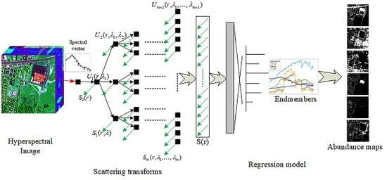
The proposed STFHU framework is illustrated in Figure 1, in which the notations are utilized to clearly illustrate the structure of the proposed method and will be discussed in Section 2. The spectral vectors are processed by the scattering transform network, which aims at extracting the high-level feature representation of the spectrum. This is achieved by using a cascade of transforms applied firstly to the input spectral vectors, which include a single pixel vector or neighborhood of the pixel vector, and then sequentially to the outputs of each transform stage. Subsequently, the features are used as the input to the regression model, and the abundance of the spectrum is then obtained. The scattering transforms are typically implemented using wavelet functions (known as wavelet scattering transforms) but other transforms are also possible (for example, the Fourier scattering transform).
2.1. Pixel-Based Wavelet Scattering Transform
Let be a wavelet cluster, which is scaled by from the mother wavelet, and it can be shown as:
and then a wavelet modular operator is defined, which includes the wavelet arithmetic and modular arithmetic,
where the first part, , is called scattering coefficient and represents the main information at low frequency bands of the input signal, while the second part, , is the scattering propagator, which is the model of the nonlinear wavelet transform. is the coefficient output of each different order, and is the input to the transform of the next order, used to regain the high frequency information. is the spectral vector input, and represents the variables in wavelet modular operator. Moreover, the scaling function is . Figure 1 shows the J = 3.
In this way, the scattering transform constructs invariable, stable, and abundant signal information by utilizing iterative wavelet decomposition, a modulus operation, and a low pass filter. The zero-order scattering transform output is:
and then can be used as the input to the first-order transform:
In addition, the first-order scattering transform output and the corresponding input are:
Finally, a collection of the scattering transform coefficient outputs from zero-order to mth-order can be obtained as:
which is the scattering transform feature vector for the hyperspectral pixel . The main advantages of scattering transforms include the translation invariance, local deformation stability, energy conservation, and strong anti-noise ability.
2.2. 3D-Based Scattering Transform
As the mixture in one pixel usually includes land cover that is around the pixel, the spatial information is crucial for hyperspectral image processing and should be taken into account in spectral unmixing.
The spectral vector at location in spatial coordinates is given as:
and in order to extract the spectral–spatial information, a 3D filter is utilized to compute the data cube of hyperspectral images. Because the spectral information is the major information for unmixing, is firstly assumed where f(p,q)f(p,q,o). As shown in Figure 2, the filter with the size of is represented, and the new data cube after being filtered is:
where are the neighbors of , while are the coefficients of the filter. In this paper, the average filter is used to construct the new cube.
Compared with , includes the spectral information and spatial information. Therefore, it can be figured out that one of the key factors in the 3D scattering transform framework for hyperspectral unmixing is designing the filter function .
From Equations (2)–(10), the scattering transform coefficients can be retrieved as:
It can be seen that the scattering transform processing framework derives features in a similar way to a CNN processing framework.
The hierarchical example spectra of the scattering transform network are demonstrated in Figure 3 and in the “scattering transform” part of Figure 1. The original spectrum of one pixel in one hyperspectral image with 156 bands is shown in the first row, while the other rows illustrate the scattering transform coefficients of this spectrum. In this instance, the parameters are set as . The coefficients in the second row, which are applied by using the low-pass filter , are very smooth and show consistency compared with the original spectrum. In the third and fourth rows, it can be found that the high frequency information is separated by . For the fourth row, the high-pass scattering transform value is very low; therefore, only the three low-pass information is left. Then, the scattering transform feature vector with 1092 dimensions, which comprises the seven scattering transform coefficient vectors in the above rows, is shown in the fifth row. Thus, the feature vector has richer, smoother information than the original spectrum, while maintaining a similar spectral envelope to the original spectra.
2.3. Regression Model of Scattering Transform Features
According to the scattering transform hyperspectral unmixing structure in Figure 1, the input is the spectral vector of a pixel, and the output are the abundances of endmembers. After the pixel-based or 3D-based scattering transform results are obtained, the scattering coefficients of each pixel at position can be used as scattering transform features. Therefore, the mixture model can be rewritten as:
After that, the regression model is used to predict the abundance corresponding to the endmembers of each pixel by utilizing the feature vectors. For the regression model, k-nearest neighbor (k-NN) is applied to learn a regressor based on the scattering transform features in samples for training. k-NN predicts the values of the spectra in test sets based on how closely the features resemble the spectra in the training set. As the endmembers are often considered by using the pure pixels in hyperspectral images, the operation principal of the k-NN regressor can be illustrated in Figure 4. The inputs are scattering transform features, and the outputs are abundance maps.
3. Experimental Results and Analysis
3.1. Experimental Datasets
Both synthetic and real hyperspectral datasets are used for conducting the experiments to verify advantages and efficiency of the proposed scattering transform framework for hyperspectral unmixing.
3.1.1. Synthetic Hyperspectral Dataset
Eight spectra are randomly selected as the endmembers from the United States (U.S.) Geological Survey (USGS), which is available at [41]. The endmembers are shown in Figure 5, in which the abundance matrix of the endmembers is generated by utilizing the method introduced in [42]. The size of the abundance matrix is (250 × 250 × 8) and the spectral band number is 188. The generated abundances of the eight endmembers are shown in the first column of Figure 12.
In order to verify the robustness performance of the proposed algorithm, Gaussian white noise is added to the synthetic hyperspectral data. Figure 6 shows the 100th band of the original and noisy synthetic data, and Figure 7 shows their spectra located at the (100, 100) pixel. Gaussian parameters are set by zero mean with 0.001 and 0.005 variance, respectively. The noisy synthetic hyperspectral dataset with 0.001 variance is called Noise1, and noisy dataset with 0.005 variance is called Noise2. It can be seen that Noise2 is more ambiguous than the original data and Noise1, and the spectrum of Noise2 includes a large amount of disturbance.
3.1.2. Real-World Hyperspectral Datasets
The proposed approach is applied to three real-world hyperspectral datasets, which are downloaded from [43], and the detailed explanation is provided in [44].
- (1)
- Urban data
The Urban dataset is a very popular hyperspectral dataset for unmixing studies. The images are of 307 × 307 pixels, and the spatial resolution is 2 m. Each pixel includes 162 effective channels with the wavelength ranging from 400 to 2500 nm. There are six endmembers in the dataset, including “Asphalt Road”, “Grass”, “Tree”, “Roof”, “Metal”, and “Dirt”. Figure 8 shows the endmembers of the Urban dataset, and the Urban dataset and the ground truth of abundances of endmembers are shown in Figure 9.
- (2)
- Jasper Ridge data
Jasper Ridge is one of the most widely used hyperspectral unmixing datasets, with each image of size 100 × 100 pixels. Each pixel is recorded at 198 effective channels with the wavelength ranging from 380 to 2500 nm. There are four endmembers latent in this dataset, including “Road”, “Dirt”, “Water”, and “Tree”. The Jasper Ridge data and the ground truth abundance of endmembers are shown in Figure 10.
- (3)
- Samson data
In the Samson datasets, each image is of size 95 × 95 pixels and there are 156 channels covering the wavelengths from 401 to 889 nm. There are three target endmembers in the dataset, including “Rock”, “Tree”, and “Water”. Figure 11 shows the Samson data and the corresponding ground truth abundances.
3.2. Experimental Setup
All of the experiments are tested on a notebook with the i7-8750H CPU, NVIDIA Quadro P4200 GPU and 32 GB RAM on Ubuntu 18.04 Linux System. The main software used includes Tensorflow [45], scikit-learn [46], and Keras [47].
In order to evaluate the performance of the proposed algorithm, there are three contrastive methods, which are ANN [24], LSU [16], and CNN [29]. Because the proposed STFHU is based on a regression model, in order to achieve effective validation, the selected contrastive methods are also based on a regression model. According to the literature [48], the most widely used methods for abundance estimation in hyperspectral unmixing are least square methods, which belong to linear spectral unmixing (LSU), and artificial neural networks methods, which belong to nonlinear spectral unmixing. CNN is the main state-of-the-art deep learning method for unmixing, and shows a good performance in abundance estimation. In addition, the similar structure between CNN and STFHU help to compare their performance in hyperspectral unmixing.
For ANN, the hidden layer size of MLP is set to 100, and the activation function is the “identity”, which is useful to test the bottleneck of linear functions. “Stochastic gradient descent” is utilized as the solver, and the learning rate is set to 0.001. For LSU, the fully constrained least squares LSU is selected. For CNN, there are four convolution layers and four sampling sub-layers in the network. The size of the convolution layers is set to 1 × 5, 1 × 4, 1 × 5, and 1 × 4, while their feature maps are set to 3, 6, 12, and 24, respectively [29]. The size of the pooling layers is assumed to be the maximum pooling operator, and 0.01 is adopted as the learning rate of CNN. The validation split parameter is set as 0.8. The training phase is 500 epochs for synthetic data and Urban data and 200 epochs are set for other real-world data, because there is not a significant performance improvement after 200 epochs. As for STFHU, the scattering transform parameters are set to J = 3 and m = 2. Considering k-NN regressor parameters, the number of neighbors is set as default to k = 5.
In order to quantitatively evaluate performances of the algorithms, the root mean square error (RMSE) and the root mean square of abundance angle distance (rms-AAD) are involved, and the RMSE is expressed as follows:
where denotes the ground truth abundance for the th pixel, is the predicted result of abundance in the th pixel, and denotes the total number of pixels. The smaller the RMSE, the better the performance of the predicted results.
Abundance angle distance (AAD) is used to measure the similarity between the ground truth of abundance and the predicted results of abundance. AAD and rms-AAD are formulated as:
To make fair comparisons, all of the methods are based on the same samples for training and testing, and the proportion of samples used for training and testing are also identical.
3.3. Experimental Results for the Synthetic Hyperspectral Data
3.3.1. Noise Data Results
In the simulated experiments, in order to verify the robustness and the performances of different methods in the presence of mixed noise, both the Noise1 and Noise2 data are applied utilizing the same training model coefficients, which are achieved by training the original data without any noise.
Figure 12 shows the abundance maps of the Noise2 dataset estimated by the proposed algorithm and the comparative methods, in which a color bar is drawn for showing the scale of color in the abundance maps. The training ratio is approximately 50%, where 31,000 pixels on the synthetic non-noise dataset are selected for learning parameters of the regressor, and the Noise2 dataset with 62,500 pixels is used for testing. The first column is the ground truth of different endmembers, and the other columns are the estimated abundance maps by different contrastive methods, respectively. It can be observed that by using ANN and CNN, not all endmembers in the abundance maps could be identified clearly, which indicates high sensitivity to the Gaussian noise of these two methods. LSU can help to achieve desirable abundance maps of a part of the endmembers, but the results are still not satisfying. In comparison, the proposed STFHU approach obtains unmixing results that are generally closer to the ground truth than the other state-of-the-art algorithms, and all estimated abundance maps of the eight endmembers in noisy hyperspectral data are satisfying and stable. This is because the features extracted by the scattering transform can take the Gaussian white noise in different spectral bands into account with the low-pass and high-pass filters.
In addition, the RMSE values achieved by comparing the abundance maps estimated by each aforementioned algorithm with the ground truth are illustrated in Figure 13. It can be seen that the proposed method has less RMSE than the ANN and CNN. Although LSU results in minimum RMSE values, this method results in more impulse noise, as shown in the visual results for LSU in Figure 12. Moreover, the CNN approach shows a large fluctuation in the RMSE results of Figure 13, while the proposed STFHU approach achieves stable results for all endmembers.
Table 1 demonstrates the comparison of RMSE and rms-AAD results based on three types of hyperspectral synthetic dataset, which include the original, Noise1, and Noise2, calculated by using the STFHU approach. The training model trains by original data at a training ratio of 50%. It can be found that all of the synthetic data types can achieve stable RMSE values across all eight endmembers (EMs). Moreover, the results of the fourth row in Table 1 correspond to the abundance maps in Figure 12, and they achieve an average unmixing result of 0.0894 and an rms-AAD result of 0.4655. In order to present the results in a more visible way, the eighth endmember is selected as an instance, of which the estimated abundance maps based on the three datasets are shown and compared with the ground truth in Figure 14. It further shows that our method can obtain good results in Gaussian white noise hyperspectral datasets.
3.3.2. Results When Using Different Proportions of Samples Used for Training
In order to investigate the influences of the proportions of samples used for training on the hyperspectral image unmixing performance, experiments are used to test various training ratios with all other initial conditions remain identical.
Figure 15 illustrates that the proposed approach achieves accurate abundance map estimation when there is no noise added to the original data. As for the noisy images, the RMSE values remain stable with the decrement of the training ratio, which indicates that the hyperspectral unmixing approach based on the scattering transform can utilize a small proportion (5%) of samples to train, while obtaining approximate results compared with that based on a larger percentage of samples. Thus, the proposed algorithm shows stable performances and is robust against noise, even when the training ratio is small.
To further evaluate the performance of the proposed method, performance comparisons are completed considering two contrastive approaches, including the CNN and ANN, which are shown in Table 2.
To further compare the proposed algorithm with the state-of-the-art CNN in hyperspectral unmixing, the ground truth, as well as the estimated abundance maps, utilizing 5% samples for training based on both algorithms and non-noisy data are shown in Figure 16. Taking Endmember 2, which presents large RMSE differences, as an example, it can be observed that the proposed method based on scattering transform possesses advantages in showing details of the ground truth, thus having closer predictions to the ground truth. The CNN algorithm leads to unsharpness in these abundance map estimates, which means the robustness to noise and the performance stability when using different proportions of samples for training are both unsatisfactory.
3.4. Experimental Results for Real-World Hyperspectral Data
3.4.1. Results of Experiment Based on the Urban Dataset
Table 3 shows the unmixing results of the proposed pixel-based scattering transform method and contrastive methods by using multiple training ratios, including 50%, 10%, and 5%. The results with blue background correspond to the proposed algorithm, while the orange, pink, and green colored backgrounds represent the RMSE values obtained by utilizing CNN, LSU and ANN separately.
Comparative results of abundance map estimation of the Asphalt Road and Dirt endmembers utilizing the proposed STFHU method, ANN, LSU, and CNN are shown in Figure 17. From Table 3 and Figure 17, it can be seen that the proposed algorithm achieves better average RMSE in predicting the abundance maps, which is a considerable improvement over other contrastive methods. It can be seen that it is difficult for the LSU approach to accurately complete the unmixing in real-world data. ANN does not obtain ideal results either, which have large differences compared with the ground truth. Figure 18 makes these disadvantages visible in terms of showing light green color in most parts of the pixels, which should be blue in the ground truth, indicating degradations in the prediction performance and adaptiveness to the real-world data. CNN can help to achieve better RMSE results compared with LSU and ANN, but different network structures in CNN can lead to large variations of the experimental results. The pixel-based CNN obtains an average of RMSE value of 0.0456 considering urban hyperspectral data unmixing, while the pixel-based scattering transform approach proposed in this paper achieves a more accurate average RMSE of 0.0301.
Figure 18 illustrates comparisons of the abundance maps estimated by the proposed STFHU and the CNN method, both of which are pixel-based. It is clear that the estimated result of endmember “metal” using CNN has a large difference to the ground truth, while the method proposed in this paper achieves results that more closely match the ground truth. When analyzing Figure 19 in detail, the square-shaped object in the top right corner should be predicted as part of the Roof endmember, but CNN estimates this as a share of the Asphalt Road and Roof. Overall, the proposed method achieves accurate estimated abundance maps for all endmembers using a low training ratio, which is better than the CNN results.
3.4.2. Results of Experiments Based on the Jasper Ridge and Samson Datasets
Table 4 and Table 5 list the RMSE results of hyperspectral unmixing utilizing the proposed method and three contrastive approaches based on the Jasper Ridge and Samson datasets. Due to the small amount of data, the condition of 75% training ratio is analyzed. It can be found that the proposed algorithm achieves better RMSE results in all cases compared with CNN, LSU, and ANN. In particular, the proposed method obtains average RMSE results for the two datasets of 0.0215 and 0.0150, respectively, which are much smaller than the other contrastive values. These comparisons further demonstrate advantages of the proposed approach in hyperspectral unmixing based on a small amount of data for training.
4. Discussion
The above experimental results show that the proposed pixel-based STFHU method can obtain good performance in HIS unmixing. In this section, we would like to discuss the robustness to noise, effect of limited training samples, computational complexity of the proposed method, and preliminary 3D-based STFHU.
- (1)
- Robustness to noise
According the results in Section 3, the method proposed in this paper is more robust to random noise interference in the remote sensing image and more adaptable to the environment, which brings benefits in effectively solving the problem of spectral variability caused by the variety of endmembers.
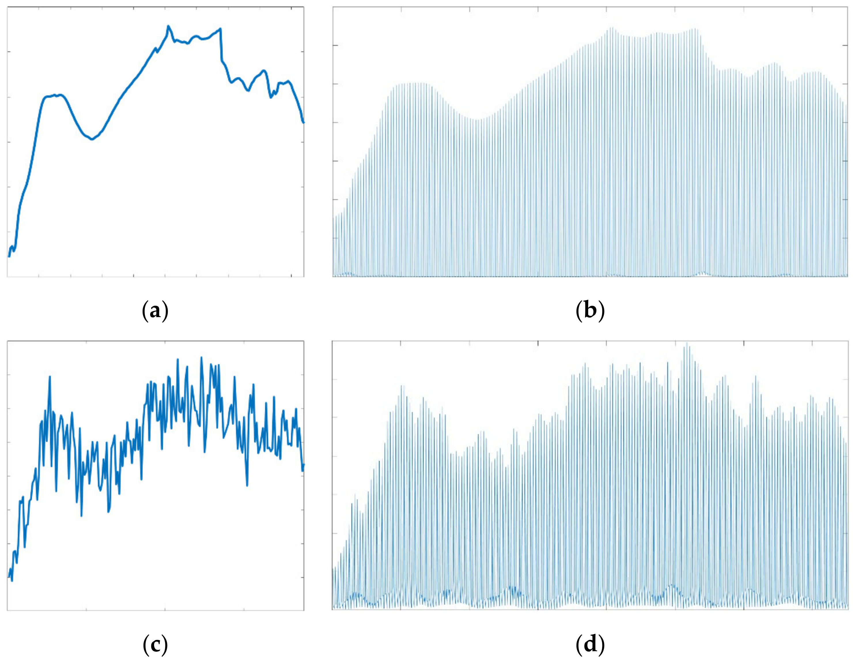
Figure 19 illustrates the advantages of the scattering transform approach in extracting reliable features from noisy hyperspectral data. Figure 19a,c plots the original spectral and Noise2 spectral data, which have a mathematical expectation of zero and a variation of 0.005, separately. Figure 19b,d delineates the curves of scattering transform features extracted from the original data and Noise2, respectively. By comparing Figure 19b,d, it can be seen that the overall information carried by the noisy image and the original image present excellent consistency, which means that the transformed noisy spectral data can reflect the information of the non-noisy component of the mixed signal well. Therefore, the scattering transform features entail benefits in effectively reducing the effects of white noise so that the accuracy of hyperspectral unmixing can be improved.
- (2)
- Effect of limited training samples
When the number of samples used for training is relatively high, it is easier to achieve excellent unmixing results, while in real-world scenarios, the samples for training can be difficult to obtain, which makes it meaningful to compare the performances when there are limited numbers of samples for training.
Table 2 compares the RMSE values when estimating the abundance maps of eight endmembers using non-noisy hyperspectral simulated data and three algorithms at different training ratios, including 10% and 5%. In both training ratios, the average RMSE of the CNN algorithm is higher than the other two methods, indicating a high demand of large numbers of training data. When 5% samples are utilized for training, the performance of CNN is worse than that of the 10% condition. Moreover, compared with the ANN method, the algorithm proposed in this paper presents lower average RMSE and rms-AAD results at both training ratios. When the training ratio decreases from 10 to 5%, the average RMSE of STFHU has a 20% increase from 0.0340 to 0.0408, while the average RMSE of ANN increases by 43.47% from 0.0421 to 0.0604.
In addition, from the results for 10% and 5% training ratios in Table 3, the proposed method achieves an average RMSE of 0.0790 at a training ratio of 5%, which is better than the CNN average RMSE result of 0.0818 at a training ratio of 10%. Additionally, it also precedes 0.1165 for LSU and 0.1415 for ANN utilizing 50% samples for training. These results demonstrate the unmixing ability of the proposed method when the proportion of samples for training is small, which shows equivalent or better results than the contrastive approaches using 50% of samples for training.
This proves that when there are limited samples for training, the proposed approach shows more apparent advantages in hyperspectral unmixing than other contrastive methods.
- (3)
- Discussion of computational complexity
It is necessary to train a considerable number of samples for building regression models, but our proposed method just needs to calculate the feature coefficient. Therefore, this framework can reduce the time cost. In this part, we mainly discuss the computational complexity of STFHU, LSU, ANN, and CNN.
From [49], we can obtain that the scattering coefficients are calculated with . In [50], the complexity of k-NN is , where n is the cardinality of the training set and d is the dimension of each sample. As the proposed STFHU is composed of scattering transforms and k-NN regression, the total computational complexity is .
Based on [51], the computational complexity of least square regression is .
The time computational complexity of the CNN can be computed by , where m is the length of feature map side, is the length of convolution kernel side, is the number of input channels, is the number of output channels, D is the number of convolution layers, and represents the th convolution layer. According to [52], the computational complexity of the CNN can be shown to be , which is the same as the complexity of the ANN method.
Therefore, it can be seen that the computational complexity of STFHU is much smaller than that of the least square regression,, and CNN and ANN, . Hence, the proposed method is significantly more computationally efficient than the comparative methods when using the same amount of training samples.
Furthermore, using the CNN requires modification of the network structure and parameters, such as the convolution layers, pooling layers, learning rate, and epochs, to optimize the performance for different training datasets, resulting in time-consuming training phases. In comparison, the proposed algorithm requires fewer parameters, including J and m, and the implementation of the k-NN regressor utilizing default settings achieves satisfactory performance, whilst different settings do not lead to significant changes in the performance. It means that our STFHU is less dependent on parameter choices. Thus, the method proposed in this paper shows advantages in simplifying the network structure and increasing the efficiency of computation.
- (4)
- Discussion of the preliminary 3D-based STFHU results
3D-based approaches have been validated to be useful for HIS processing, which is preliminarily taken into account in this paper. Table 6 shows the average RMSE (Avg-RMSE) and rms-AAD results of unmixing utilizing both pixel-based and 3D-based scattering transform approaches based on small amounts of urban image samples for training. It can be observed that the average RMSE and rms-AAD of unmixing results become larger as the training ratio decreases using the same methods. To solve problems involved by utilizing a small proportion of samples for training, the 3D-based scattering transform is proposed, especially for real-world hyperspectral unmixing. Considering the effects on single-pixel spectral curve caused by the environment, the 3D spatial information can enrich the information included in the curve, thus being practical for real-world applications. In Table 6, the average RMSE using the 3D-based scattering transform at a training ratio of 0.5% is 0.1584, while the value for the pixel-based approach is 0.2148, which is larger than 0.1912, the result at 0.3% training ratio utilizing the 3D-based method. Likewise, the 3D-based approach can achieve equivalent rms-AAD at 0.5% training ratio compared with the result when using a training ratio of 2% for the pixel-based method. The aforementioned results verify that the 3D spatial information can provide effective cues when using low training ratios.
In future research, this type of information will be further utilized to combine with the scattering transform features to develop new algorithms to further improve the performance of hyperspectral unmixing.
5. Conclusions
In this paper, a novel scattering transform framework is proposed to improve the accuracy of hyperspectral unmixing. The STFHU method possesses a multilayer structure for extracting features, which is similar to the structure of CNN and can increase the accuracy of describing the desired features. The pixel-based and 3D-based scattering transforms are excellently suited for hyperspectral unmixing since they not only lead to sufficient information in the extracted features, but also suppress the interference of noise. In particular, this approach is robust against Gaussian white noise and a small amount of training samples. These scattering transform techniques are then combined with the k-NN regressor to form a framework for end-to-end feature extraction and deep scattering network for abundance estimation. Compared with CNN, the proposed solution has a clear structure and few parameters, leading to better viability and efficiency of computation. Experimental results based on simulated data and three real-world hyperspectral remote sensing image datasets provide abundant evidences of the robustness and adaptiveness of the proposed approach. Under the interference of Gaussian white noise, whose variance is 0.005, the scattering transform features are helpful to achieve closer abundance map predictions of the ground truth, thus having better unmixing results than the other contrastive approaches. Moreover, based on identical data for training and testing, the proposed algorithm gains the least RMSE and rms-AAD among all investigated methods, and it can also accurately complete the unmixing task when utilizing 5% of the samples for training. In addition, this paper presents preliminary verifications of the performance of 3D-based scattering transform based on a small number of samples, which is better than that of the pixel-based approach.
Although the proposed scattering transform framework can obtain desirable performance for hyperspectral unmixing, there is still a need to further improve the utilization of spatial correlation. For the preliminary 3D-based framework in this paper, the spatial information is calculated firstly, and then we mainly use the spectral information for scattering transform. In terms of future research, we plan to investigate how to provide a whole joint spectral-spatial scattering transform framework for hyperspectral spectral image unmixing.
Author Contributions
Conceptualization, Y.Z. and C.R.; methodology, Y.Z. and C.R.; software, Y.Z.; validation, Y.Z., J.Z., and C.R.; writing—original draft preparation, Y.Z. and J.Z.; writing—review and editing, C.R. and J.L.; funding acquisition, Y.Z.
Funding
This research was funded by the National Natural Science Foundation of China under grant number 61801018, the China Scholarship Council under grant number 201906465009, the Advance Research Program under grant number 6140452010101, and the Fundamental Research Funds for the Central Universities under grant number FRF-BD-19-002A.
Acknowledgments
The authors would like to thank the editor and reviewers for their reviews that improved the content of this paper.
Conflicts of Interest
The authors declare no conflicts of interest.
References
- Bioucas-Dias, J.M.; Plaza, A.; Camps-Valls, G.; Scheunders, P.; Nasrabadi, N.; Chanussot, J. Hyperspectral remote sensing data analysis and future challenge. IEEE Geosci. Remote Sens. Mag. 2013, 1, 6–36. [Google Scholar] [CrossRef]
- Heylen, R.; Parente, M.; Gader, P. A review of nonlinear hyperspectral unmixing methods. IEEE J. Sel. Top. Appl. Earth Obs. Remote Sens. 2014, 7, 1844–1868. [Google Scholar] [CrossRef]
- Zhou, Y.; Rangarajan, A.; Gader, P.D. A spatial compositional model for linear unmixing and endmember uncertainty estimation. IEEE Trans. Image Process. 2016, 25, 5987–6002. [Google Scholar] [CrossRef] [PubMed]
- Wang, S.; Huang, T.-Z.; Zhao, X.-L.; Liu, G.; Cheng, Y. Double Reweighted Sparse Regression and Graph Regularization for Hyperspectral Unmixing. Remote Sens. 2018, 10, 1046. [Google Scholar] [CrossRef]
- Jiang, J.; Ma, J.; Wang, Z.; Chen, C.; Liu, X. Hyperspectral Image Classification in the Presence of Noisy Labels. IEEE Trans. Geosci. Remote Sens. 2019, 57, 851–865. [Google Scholar] [CrossRef]
- Ren, H.; Chang, C.I. Automatic spectral target recognition in hyperspectral imagery. IEEE Trans. Aerosp. Electron. Syst. 2003, 39, 1232–1249. [Google Scholar]
- Li, J. Wavelet-based feature extraction for improved endmember abundance estimation in linear unmixing of hyperspectral signals. IEEE Trans. Geosci. Remote Sens. 2004, 42, 644–649. [Google Scholar] [CrossRef]
- Ghaffari, O.; Zoej, M.J.V.; Mokhtarzade, M. Reducing the effect of the endmembers’ spectral variability by selecting the optimal spectral bands. Remote Sens. 2017, 9, 884. [Google Scholar] [CrossRef]
- Zou, J.; Lan, J.; Shao, Y. A Hierarchical Sparsity Unmixing Method to Address Endmember Variability in Hyperspectral Image. Remote Sens. 2018, 10, 738. [Google Scholar] [CrossRef]
- He, W.; Zhang, H.; Zhang, L. Sparsity-Regularized Robust Non-Negative Matrix Factorization for Hyperspectral Unmixing. IEEE J. Sel. Top. Appl. Earth Obs. 2016, 9, 4267–4279. [Google Scholar] [CrossRef]
- Bioucas-Dias, J.M.; Figueiredo, M.A. Alternating direction algorithms for constrained sparse regression: Application to hyperspectral unmixing. In Proceedings of the 2nd Workshop on Hyperspectral Image and Signal Processing: Evolution in Remote Sensing, Reykjavik, Iceland, 14–16 June 2010; pp. 1–4. [Google Scholar]
- Keshava, N.; Mustard, J.F. Spectral unmixing. IEEE Signal Process. Mag. 2002, 19, 44–57. [Google Scholar] [CrossRef]
- Drumetz, L.; Veganzones, M.A.; Henrot, S.; Phlypo, R.; Chanussot, J.; Jutten, C. Blind hyperspectral unmixing using an extended linear mixing model to address spectral variability. IEEE Trans. Image Process. 2016, 25, 3890–3905. [Google Scholar] [CrossRef] [PubMed]
- Miao, X.; Gong, P.; Swope, S.; Pu, R.; Carruthers, R.; Anderson, G.L.; Heaton, J.S.; Tracy, C.R. Estimation of yellow starthistle abundance through CASI-2 hyperspectral imagery using linear spectral mixture models. Remote Sens. Environ. 2006, 101, 329–341. [Google Scholar] [CrossRef]
- Eches, O.; Dobigeon, N.; Mailhes, C.; Tourneret, J.Y. Bayesian estimation of linear mixtures using the normal compositional model. Application to hyperspectral imagery. IEEE Trans. Image Process. 2010, 19, 1403–1413. [Google Scholar] [CrossRef] [PubMed]
- Heinz, D.; Chang, C.I. Fully constrained least squares linear mixture analysis for material quantificationin in hyperspectral imagery. IEEE Trans. Geosci. Remote Sens. 2001, 39, 529–545. [Google Scholar] [CrossRef]
- Li, J.; Agathos, A.; Zaharie, D.; Bioucas-Dias, J.M.; Plaza, A.; Li, X. Minimum volume simplex analysis: A fast algorithm for linear hyperspectral unmixing. IEEE Trans. Geosci. Remote Sens. 2015, 53, 5067–5082. [Google Scholar]
- Wang, L.; Liu, D.; Wang, Q. Geometric method of fully constrained least squares linear spectral mixture analysis. IEEE Trans. Geosci. Remote Sens. 2013, 51, 3558–3566. [Google Scholar] [CrossRef]
- Yang, B.; Wang, B.; Wu, Z. Unsupervised Nonlinear Hyperspectral Unmixing Based on Bilinear Mixture Models via Geometric Projection and Constrained Nonnegative Matrix Factorization. Remote Sens. 2018, 10, 801. [Google Scholar] [CrossRef]
- Dobigeon, N.; Tourneret, J.Y.; Richard, C.; Bermudez, J.C.; McLaughlin, S.; Hero, A.O. Nonlinear unmixing of hyperspectral images: Models and algorithms. IEEE Signal Process. Mag. 2014, 31, 82–94. [Google Scholar] [CrossRef]
- Shao, Y.; Lan, J.; Zhang, Y.; Zou, J. Spectral Unmixing of Hyperspectral Remote Sensing Imagery via Preserving the Intrinsic Structure Invariant. Sensors 2018, 18, 3528. [Google Scholar] [CrossRef]
- Halimi, A.; Altmann, Y.; Dobigeon, N. Nonlinear unmixing of hyperspectral images using a generalized bilinear model. IEEE Trans. Geosci. Remote Sens. 2011, 49, 4153–4162. [Google Scholar] [CrossRef]
- Zou, J.; Lan, J. A Multiscale Hierarchical Model for Sparse Hyperspectral Unmixing. Remote Sens. 2019, 11, 500. [Google Scholar] [CrossRef]
- Foody, G.M. Relating the land-cover composition of mixed pixels to artificial neural network classification output. Photogramm. Eng. Remote Sens. 1996, 5, 491–499. [Google Scholar]
- Licciardi, G.A.; Del Frate, F. Pixel unmixing in hyperspectral data by means of neural networks. IEEE Trans. Geosci. Remote Sens. 2011, 49, 4163–4172. [Google Scholar] [CrossRef]
- Guo, R.; Wang, W.; Qi, H. Hyperspectral image unmixing using autoencoder cascade. In Proceedings of the 7th Workshop on Hyperspectral Image and Signal Processing: Evolution in Remote Sensing, (WHISPERS), Tokyo, Japan, 2–5 June 2015. [Google Scholar]
- Palsson, B.; Sigurdsson, J.; Sveinsson, J.; Ulfarsson, M. Hyperspectral unmixing using a neural network autoencoder. IEEE Access 2018, 6, 25646–25656. [Google Scholar] [CrossRef]
- Su, Y.; Marinoni, A.; Li, J.; Plaza, J.; Gamba, P. Stacked nonnegative sparse autoencoders for robust hyperspectral unmixing. IEEE Geosci. Remote Sens. Lett. 2018, 15, 1427–1431. [Google Scholar] [CrossRef]
- Zhang, X.; Sun, Y.; Zhang, J.; Wu, P.; Jiao, L. Hyperspectral unmixing via deep convolutional neural networks. IEEE Geosci. Remote Sens. Lett. 2018, 15, 1755–1759. [Google Scholar] [CrossRef]
- Arun, P.; Buddhiraju, K.; Porwal, A. CNN based sub-pixel mapping for hyperspectral images. Neurocomputing 2018, 311, 51–64. [Google Scholar] [CrossRef]
- Bouvrie, J.; Rosasco, L.; Poggio, T. On invariance in hierarchical models. In Advances in Neural Information Processing Systems; MIT Press: Whistler, BC, Canada, 11 December 2009; pp. 162–170. [Google Scholar]
- Bruna, J.; Mallat, S. Classification with scattering operators. In Proceedings of the CVPR 2011, Providence, RI, USA, 20–25 June 2011; pp. 1561–1566. [Google Scholar]
- Oyallon, E.; Belilovsky, E.; Zagoruyko, S. Scaling the scattering transform: Deep hybrid networks. In Proceedings of the IEEE International Conference on Computer Vision (ICCV), Venice, Italy, 22–29 October 2017; pp. 5618–5627. [Google Scholar]
- Pontus, W. Wavelets, Scattering Transforms and Convolutional Neural Networks, Tools for Image Processing. Available online: https://pdfs.semanticscholar.org/c354/c467d126e05f63c43b5ab2af9d0c652dfe3e.pdf (accessed on 25 August 2019).
- Andén, J.; Mallat, S. Multiscale Scattering for Audio Classification. In Proceedings of the ISMIR 2011, Miami, FL, USA, 24–28 October 2011; pp. 657–662. [Google Scholar]
- Mallat, S. Group invariant scattering. Commun. Pure Appl. Math. 2012, 65, 1331–1398. [Google Scholar] [CrossRef]
- Mallat, S. Understanding deep convolutional networks. Philos. Trans. R. Soc. 2016, 374, 20150203. [Google Scholar] [CrossRef]
- Czaja, W.; Kavalerov, I.; Li, W. Scattering Transforms and Classification of Hyperspectral Images. In Algorithms and Technologies for Multispectral, Hyperspectral, and Ultraspectral Imagery XXIV; International Society for Optics and Photonics: Orlando, FL, USA, 2018; p. 106440H. [Google Scholar]
- Tang, Y.; Lu, Y.; Yuan, H. Hyperspectral image classification based on three-dimensional scattering wavelet transform. IEEE Trans. Geosci. Remote Sens. 2014, 53, 2467–2480. [Google Scholar] [CrossRef]
- Ilya, K.; Li, W.; Czaja, W.; Chellappa, R. Three Dimensional Scattering Transform and Classification of Hyperspectral Images. 2019. Available online: https://arxiv.org/pdf/1906.06804.pdf (accessed on 12 September 2019).
- USGS Digital Spectral Library. Available online: http://speclab.cr.usgs.gov/spectral-lib.html (accessed on 10 August 2019).
- Miao, L.; Qi, H. Endmember extraction from highly mixed data using minimum volume constrained nonnegative matrix factorization. IEEE Trans. Geosci. Remote Sens. 2007, 45, 765–777. [Google Scholar] [CrossRef]
- Hyperspectral Unmixing Datasets & Ground Truths. Available online: http://www.escience.cn/people/feiyunZHU/Dataset_GT.html (accessed on 10 August 2019).
- Zhu, F.; Wang, Y.; Xiang, S.; Fan, B.; Pan, C. Structured sparse method for hyperspectral unmixing. ISPRS J. Photogram. Remote Sens. 2014, 88, 101–118. [Google Scholar] [CrossRef]
- TensorFlow Software. Available online: https://www.tensorflow.org (accessed on 20 July 2019).
- Scikit-Learn Software. Available online: https://scikit-learn.org (accessed on 20 July 2019).
- Keras Software. Available online: https://keras.io (accessed on 20 July 2019).
- Lan, J.; Zou, J.; Hao, Y.; Zeng, Y.; Zhang, Y.; Dong, M. Research progress on unmixing of hyperspectral remote sensing imagery. J. Remote Sens. 2018, 22, 13–27. [Google Scholar]
- Andén, J.; Mallat, S. Deep scattering spectrum. IEEE Trans. Signal Process. 2014, 62, 4114–4128. [Google Scholar] [CrossRef]
- CS840a Machine Learning in Computer Vision. Available online: http://www.csd.uwo.ca/courses/CS9840a/Lecture2_knn.pdf (accessed on 17 November 2019).
- Computational Complexity of Least Square Regression Operation. Available online: https://math.stackexchange.com/questions/84495/computational-complexity-of-least-square-regression-operation (accessed on 17 November 2019).
- Computational Complexity of Neural Networks. Available online: https://kasperfred.com/series/computational-complexity/computational-complexity-of-neural-networks (accessed on 17 November 2019).
Figure 1.
Structure of the hyperspectral unmixing with scattering transform features. The green arrows represent the scattering coefficient, and the black arrows delineate the scattering propagator, which is computed iteratively.
Figure 1.
Structure of the hyperspectral unmixing with scattering transform features. The green arrows represent the scattering coefficient, and the black arrows delineate the scattering propagator, which is computed iteratively.

Figure 2.
Structure of the three-dimensional (3D) filter for hyperspectral unmixing.
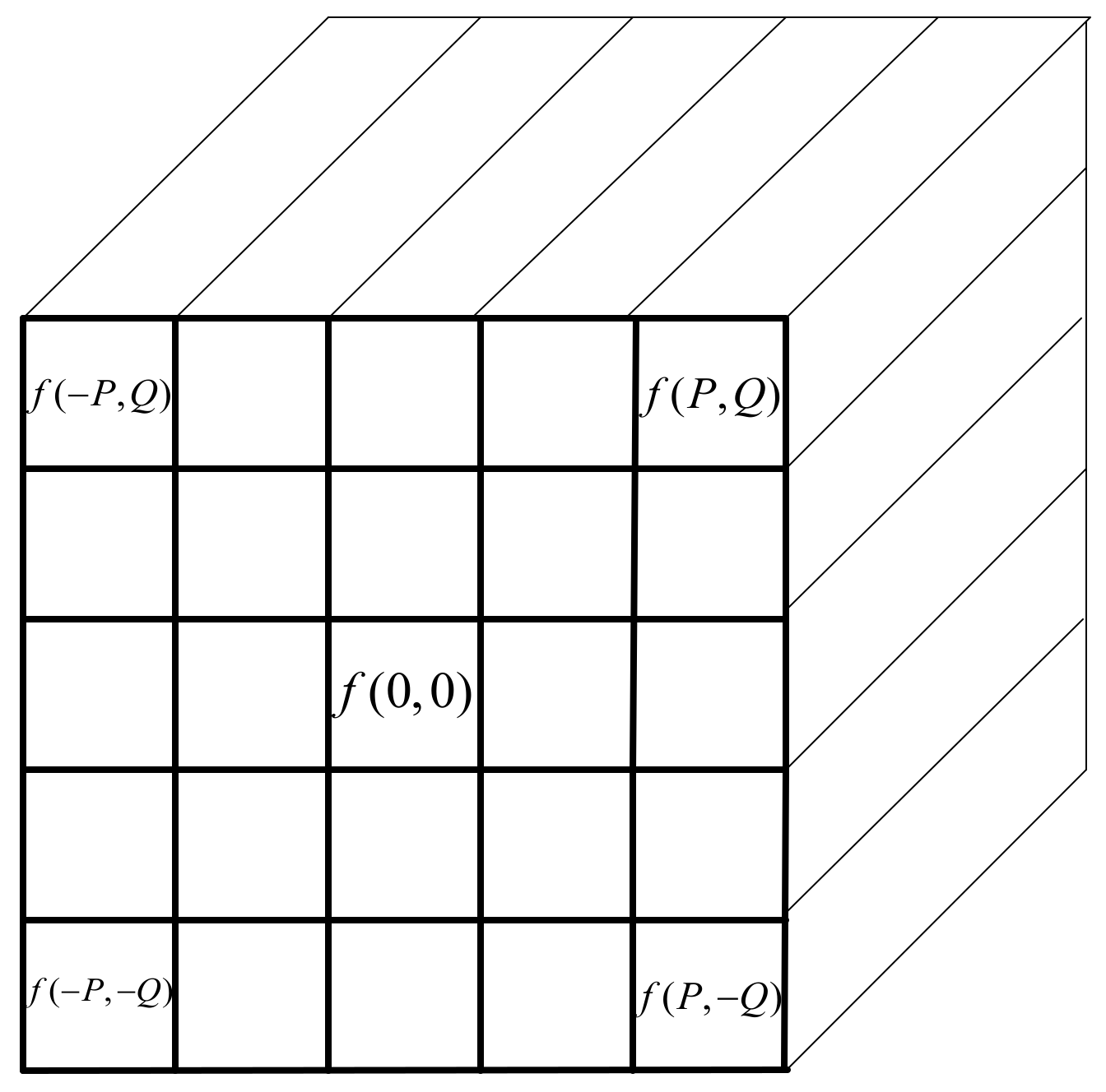
Figure 3.
Example spectra of the scattering transform network. (a) The original spectral vector input; (b) The scattering transform level 0, which is a low-pass version of the input; (c) The scattering transform level 1 and each representing 1/3 of the range of the low pass version; (d) The scattering transform level 2; and (e) The scattering transform coefficients, which consist of the scattering transform levels 0, 1, and 2.
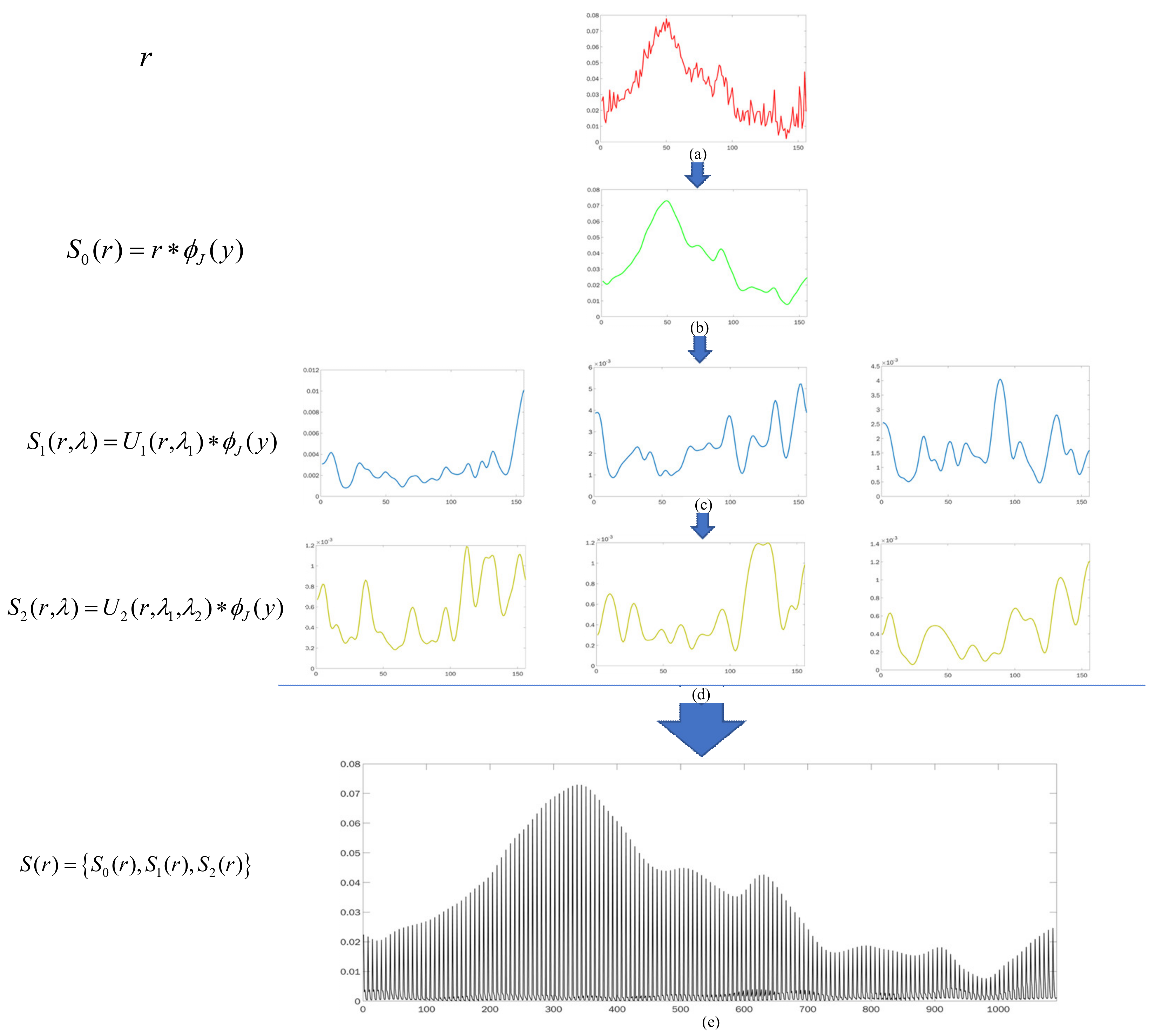
Figure 4.
Operation principal of the k-nearest neighbor (k-NN) regressor.
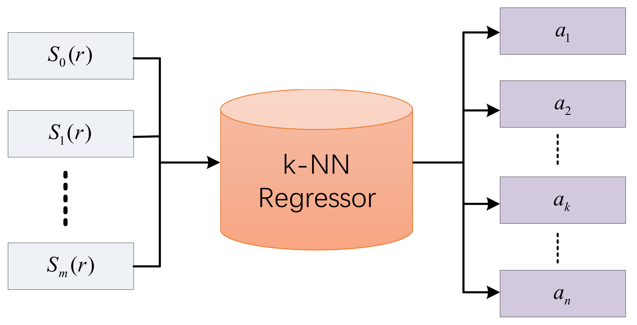
Figure 5.
Eight selected endmembers from the United States (U.S.) Geological Survey (USGS) for building synthetic data.
Figure 5.
Eight selected endmembers from the United States (U.S.) Geological Survey (USGS) for building synthetic data.
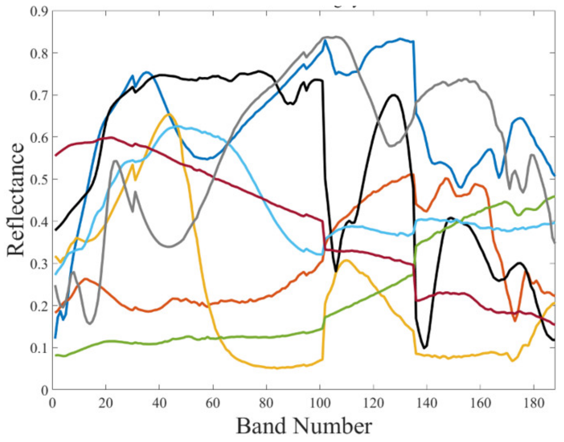
Figure 6.
Original and noisy synthetic data at the 100th band. (a) The original synthetic data at the 100th band; (b) The Noise1 data at the 100th band; and (c) The Noise2 data at the 100th band.
Figure 6.
Original and noisy synthetic data at the 100th band. (a) The original synthetic data at the 100th band; (b) The Noise1 data at the 100th band; and (c) The Noise2 data at the 100th band.
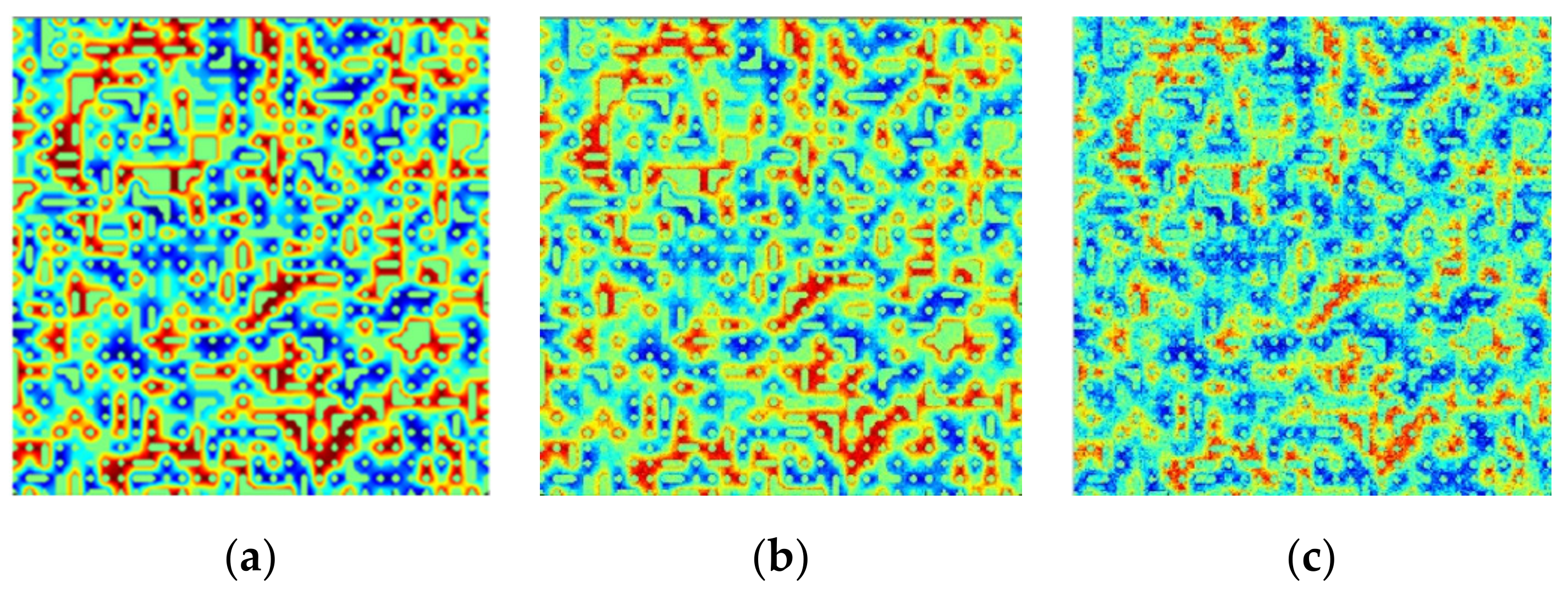
Figure 7.
Spectra of the original and noisy synthetic data located at the (100, 100) pixel. (a) The spectrum of the original synthetic data; (b) The spectrum of Noise1; and (c) The spectrum of Noise2.
Figure 7.
Spectra of the original and noisy synthetic data located at the (100, 100) pixel. (a) The spectrum of the original synthetic data; (b) The spectrum of Noise1; and (c) The spectrum of Noise2.
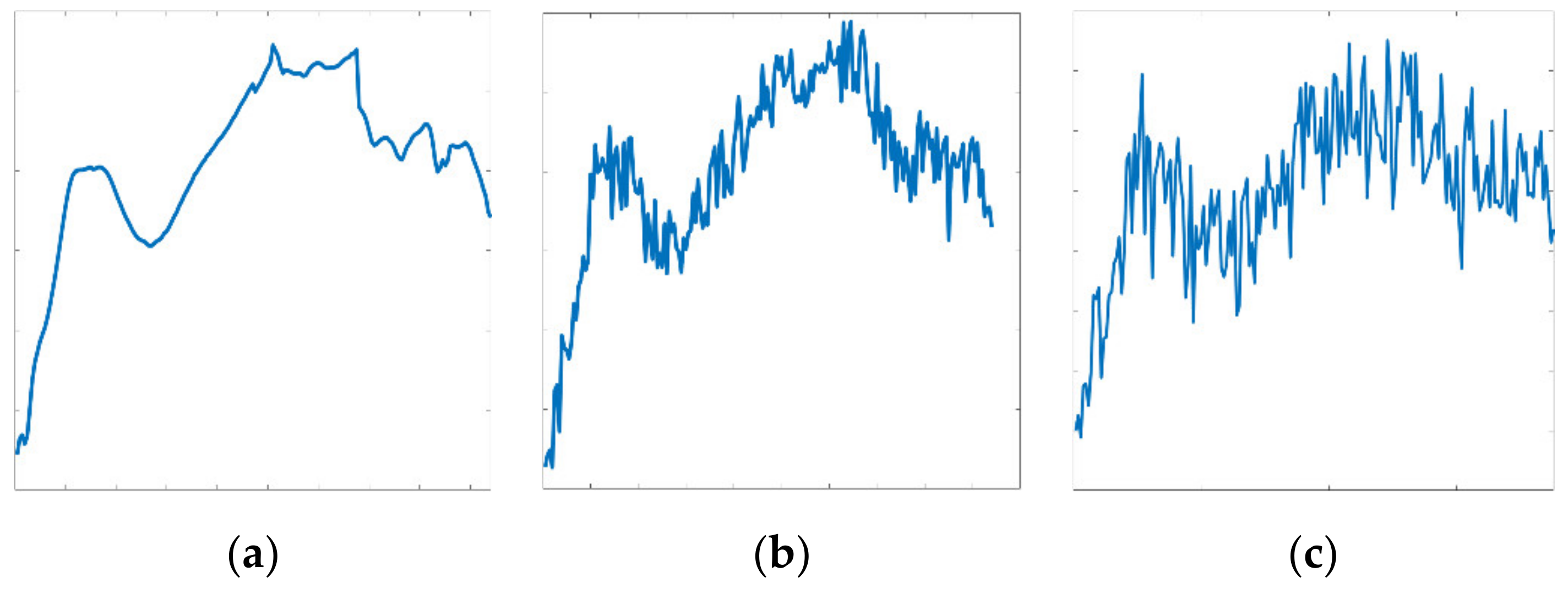
Figure 8.
Spectra plots of six endmembers of one hyperspectral image in the Urban dataset.
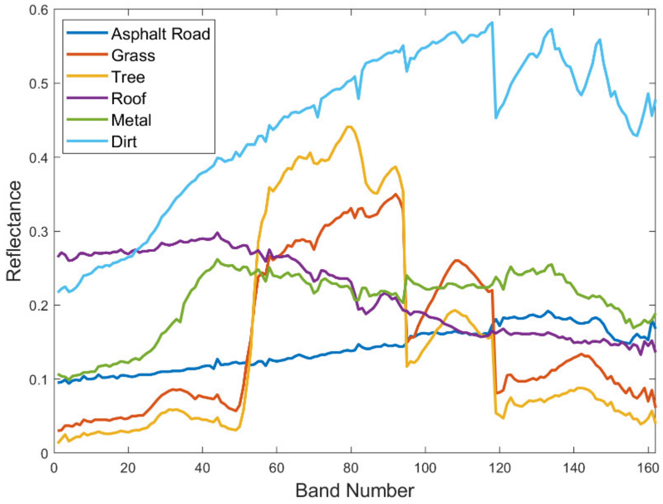
Figure 9.
Urban hyperspectral data and its ground truth. (a) The hyperspectral image and (b) the ground truth abundance maps.
Figure 9.
Urban hyperspectral data and its ground truth. (a) The hyperspectral image and (b) the ground truth abundance maps.
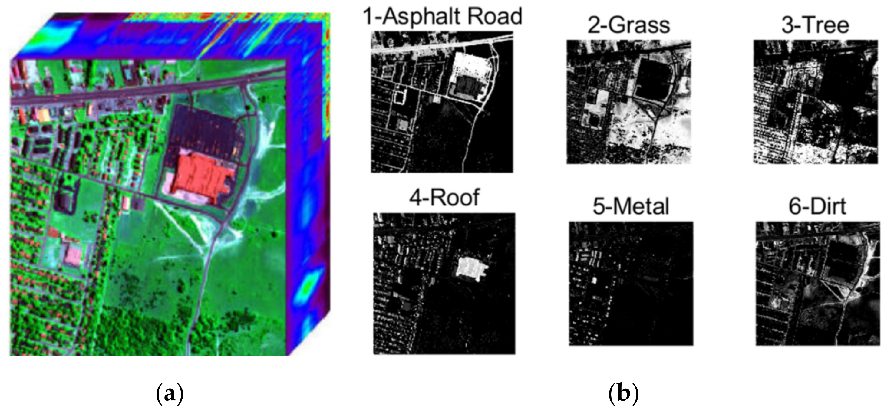
Figure 10.
Jasper Ridge hyperspectral data and its ground truth. (a) The hyperspectral image in Jasper Ridge and (b) the ground truth of abundance maps.
Figure 10.
Jasper Ridge hyperspectral data and its ground truth. (a) The hyperspectral image in Jasper Ridge and (b) the ground truth of abundance maps.
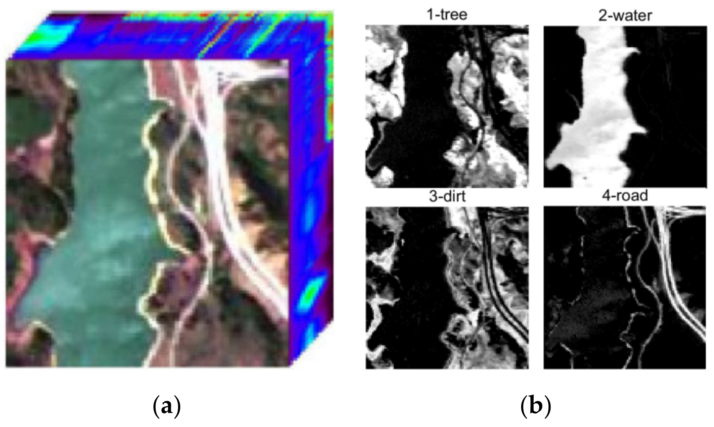
Figure 11.
Samson hyperspectral data and the ground truth. (a) Is the hyperspectral image in Samson, and (b) shows the ground truth of abundance maps.
Figure 11.
Samson hyperspectral data and the ground truth. (a) Is the hyperspectral image in Samson, and (b) shows the ground truth of abundance maps.
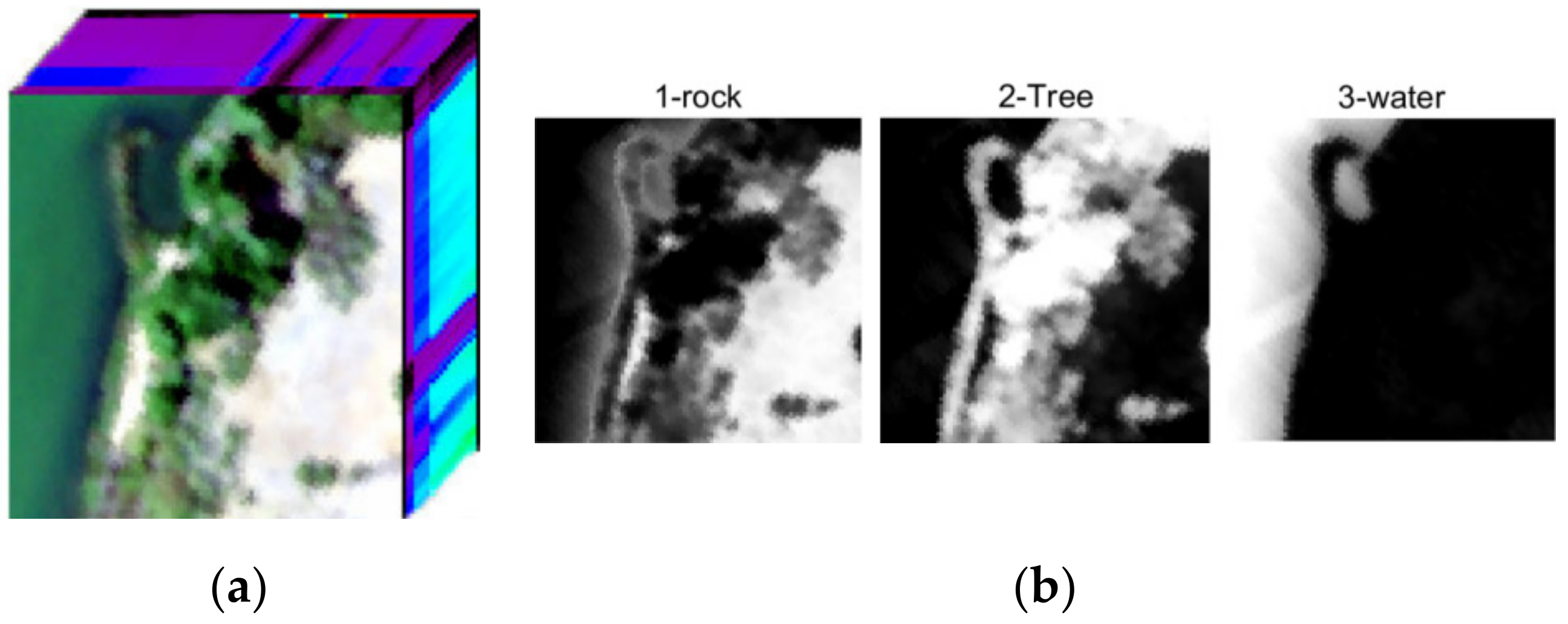
Figure 12.
Ground truth and estimated abundance maps of eight endmembers utilizing four algorithms on the Noise2 dataset at a training ratio of 50%. (a) The ground truths of all endmembers; (b) The estimated abundance maps of the proposed STFHU approach; (c) The estimated abundance maps of the ANN method; (d) The estimated abundance maps of the LSU algorithm; and (e) The estimated abundance maps of the CNN approach.
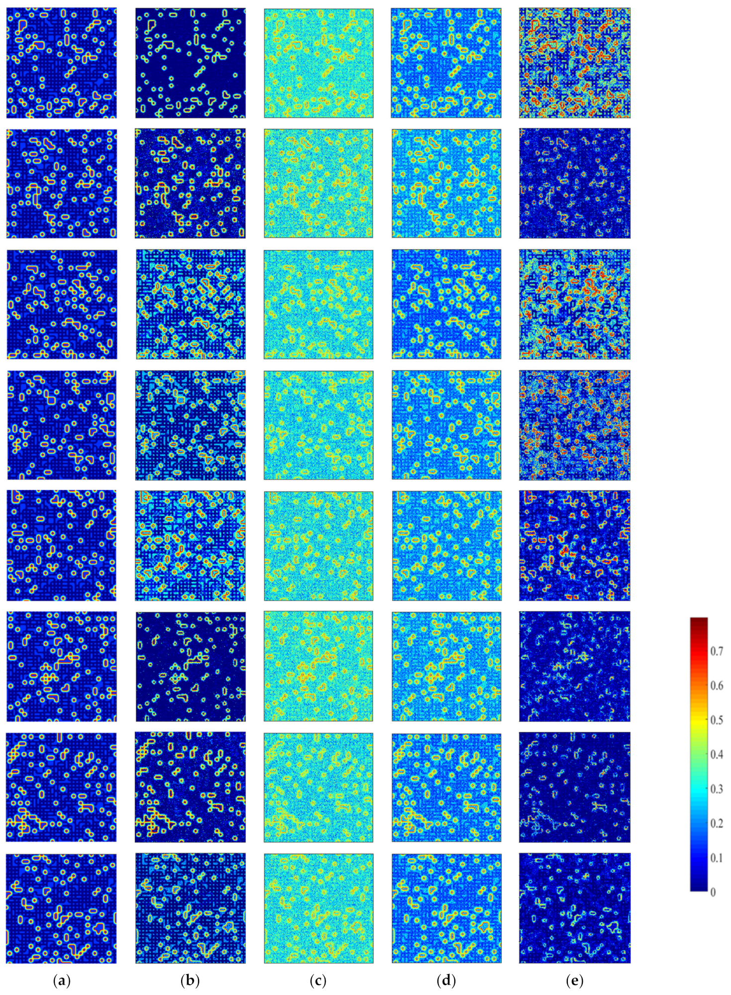
Figure 13.
RMSE values calculated by comparing the abundance maps of eight endmembers estimated by the proposed STFHU algorithm, ANN, LSU, and CNN separately with the ground truth.
Figure 13.
RMSE values calculated by comparing the abundance maps of eight endmembers estimated by the proposed STFHU algorithm, ANN, LSU, and CNN separately with the ground truth.
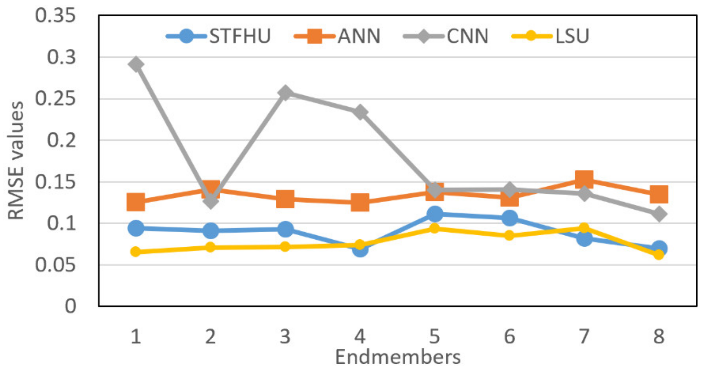
Figure 14.
Example endmember abundance map estimates of original and noisy datasets using the same non-noisy training model at a training ratio of 50%, and their comparison with the ground truth. (a) The ground truth of eighth endmembers; (b) The estimated abundance map of the original synthetic data; (c) The estimated abundance map of Noise1; and (d) The estimated abundance map of Noise2.
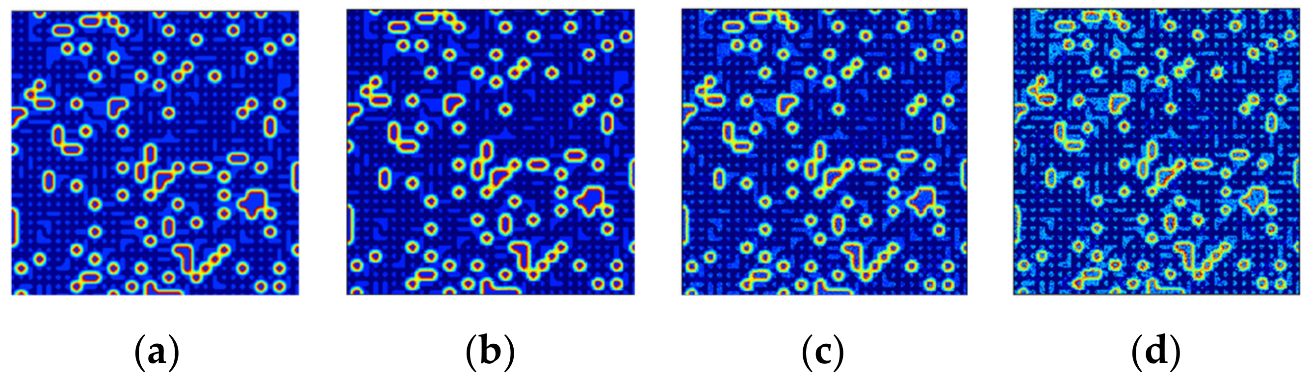
Figure 15.
Average RMSE results from comparing abundance map estimates utilizing STFHU algorithm based on the original and noisy datasets with the ground truth at different training ratios.
Figure 15.
Average RMSE results from comparing abundance map estimates utilizing STFHU algorithm based on the original and noisy datasets with the ground truth at different training ratios.
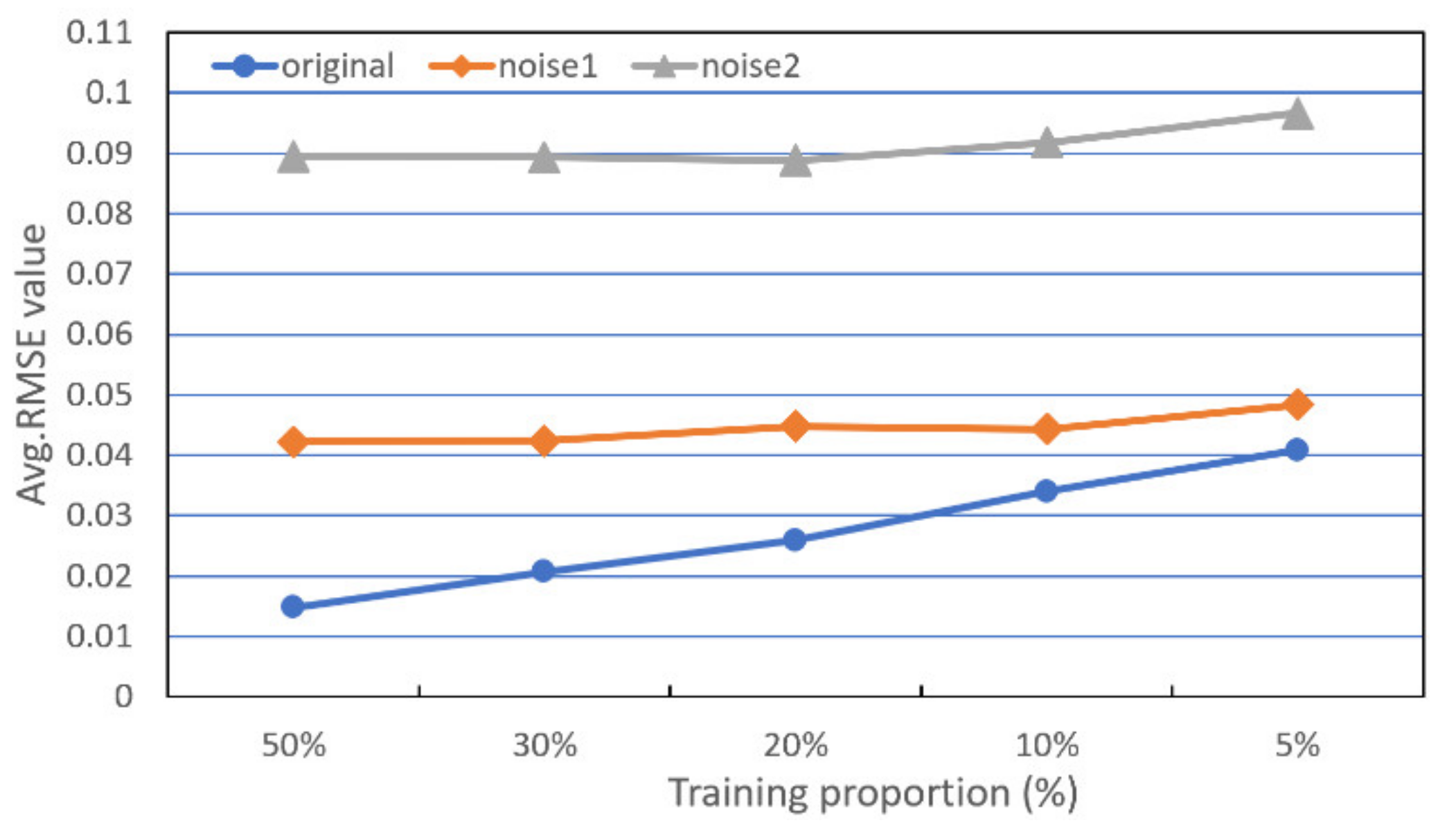
Figure 16.
Comparison of the ground truth and estimated abundance maps of the second endmember using the proposed approach and CNN separately based on non-noisy data at a training ratio of 5%. (a) The ground truth; (b) The abundance map of the proposed method; and (c) The abundance map of CNN.
Figure 16.
Comparison of the ground truth and estimated abundance maps of the second endmember using the proposed approach and CNN separately based on non-noisy data at a training ratio of 5%. (a) The ground truth; (b) The abundance map of the proposed method; and (c) The abundance map of CNN.
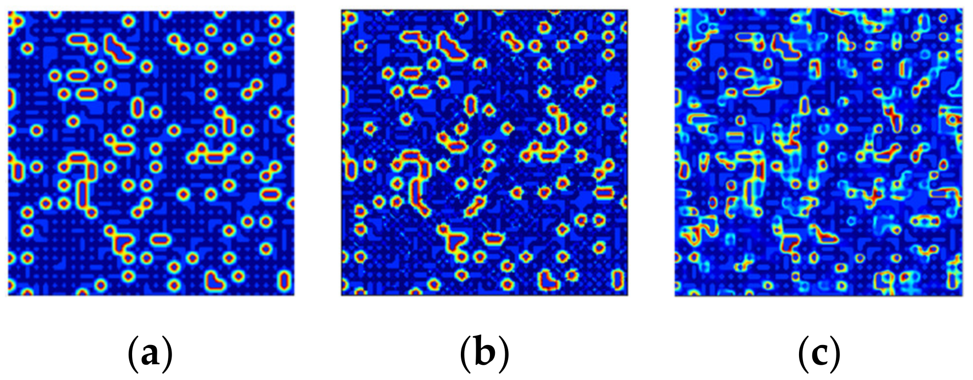
Figure 17.
Partial abundance map estimation results at a training ratio of 50%. (a) The ground truths of all endmembers; (b) The estimated abundance maps of STFHU; (c) The estimated abundance maps of the ANN method; (d) The estimated abundance maps of the LSU algorithm; and (e) The estimated abundance maps of the CNN approach.
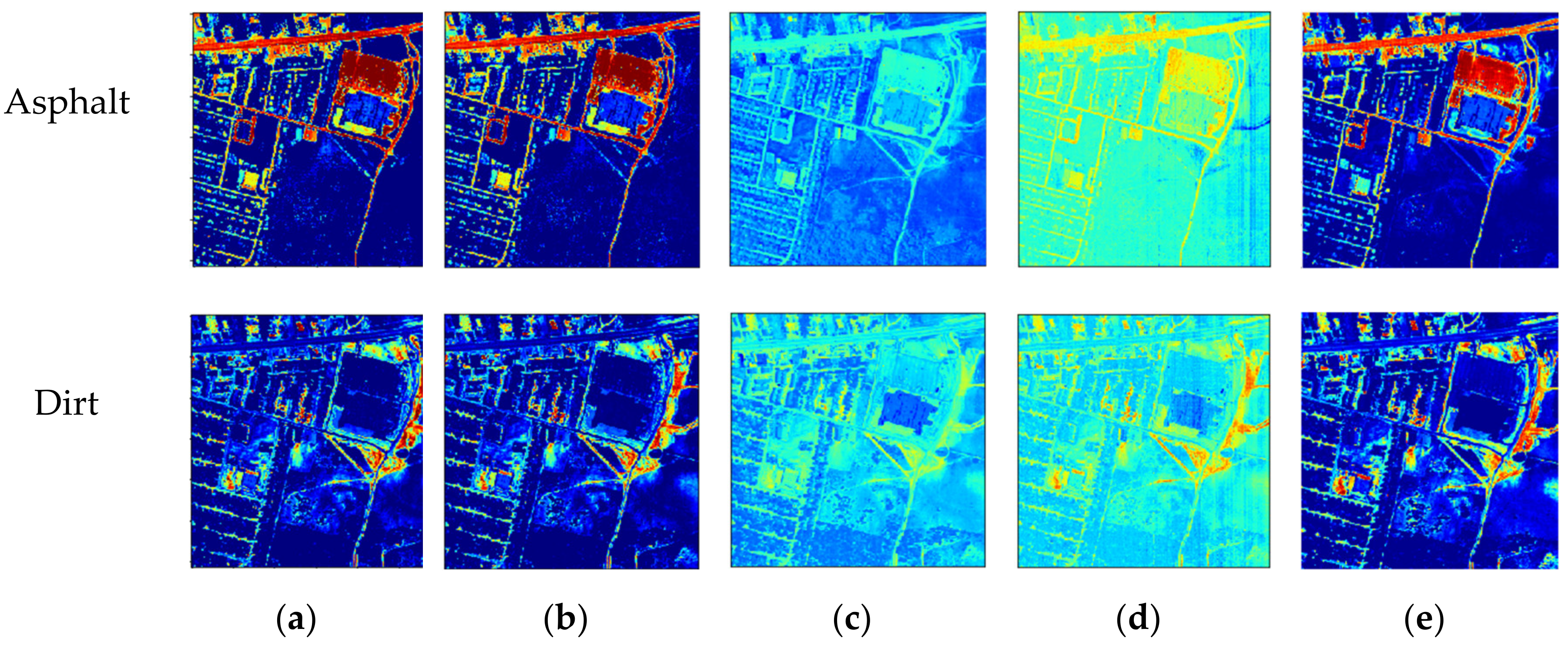
Figure 18.
Abundance map estimation results at 5% training ratio utilizing the proposed algorithm and CNN based on pixels. (a) The ground truths of all endmembers; (b) the estimated abundance maps of the proposed STFHU; and (c) the estimated abundance maps of the CNN method.
Figure 18.
Abundance map estimation results at 5% training ratio utilizing the proposed algorithm and CNN based on pixels. (a) The ground truths of all endmembers; (b) the estimated abundance maps of the proposed STFHU; and (c) the estimated abundance maps of the CNN method.
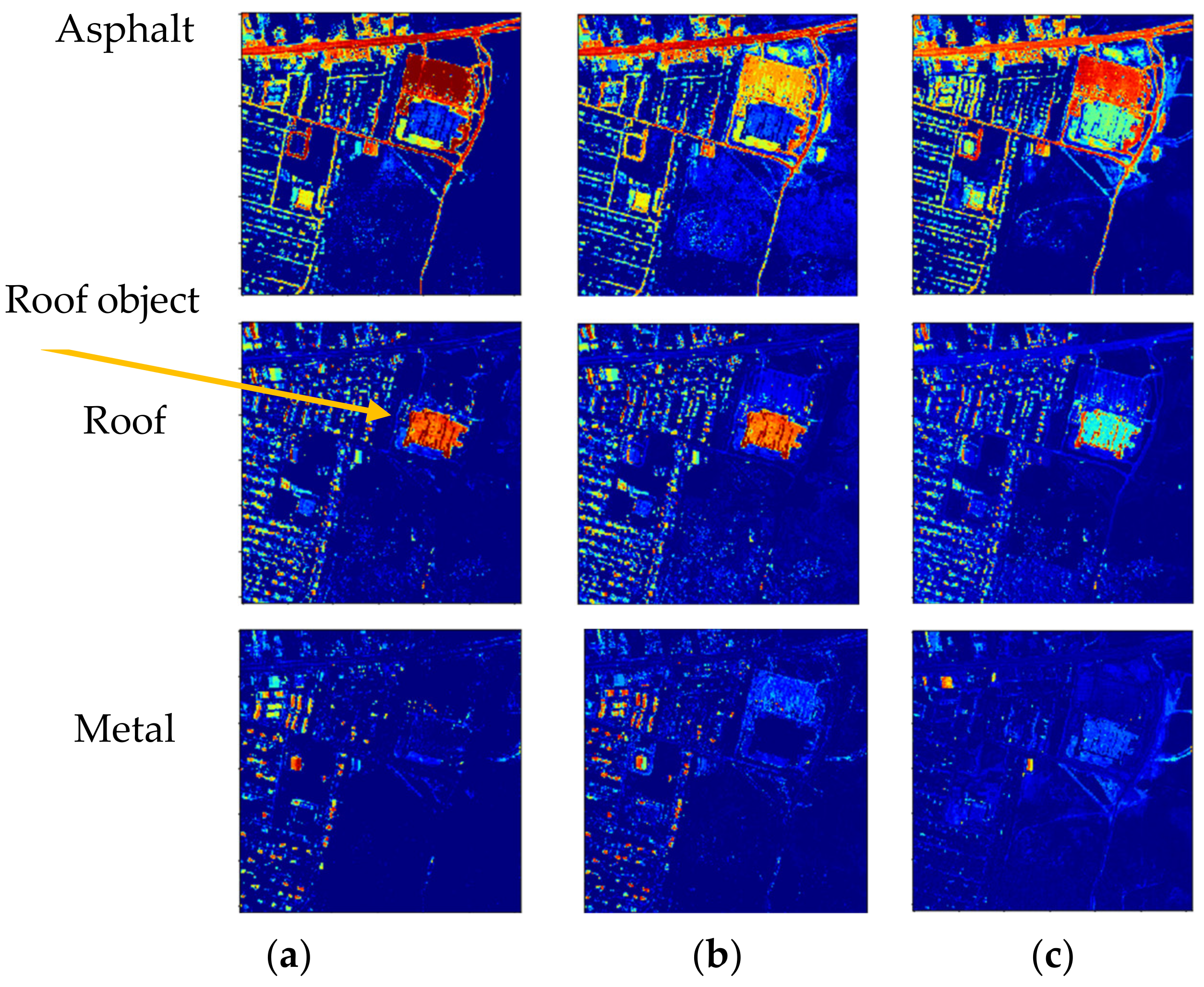
Figure 19.
Comparisons of the original spectrum and noisy spectral data with their scattering transform features. (a) The original spectrum; (b) The scattering transform features of the original spectrum; (c) The Noise2 spectrum; and (d) The scattering transform features of the Noise2 spectrum.
Figure 19.
Comparisons of the original spectrum and noisy spectral data with their scattering transform features. (a) The original spectrum; (b) The scattering transform features of the original spectrum; (c) The Noise2 spectrum; and (d) The scattering transform features of the Noise2 spectrum.

Table 1.
Comparison of the RMSE results calculated by utilizing STFHU at a training ratio of 50%.
| EM-1 | EM-2 | EM-3 | EM-4 | EM-5 | EM-6 | EM-7 | EM-8 | Avg. | Rms-AAD | |
|---|---|---|---|---|---|---|---|---|---|---|
| Original | 0.0120 | 0.0169 | 0.0121 | 0.0140 | 0.0139 | 0.0190 | 0.0176 | 0.0127 | 0.0148 | 0.0688 |
| Noise1 | 0.0441 | 0.0458 | 0.0415 | 0.0411 | 0.0379 | 0.0482 | 0.0424 | 0.0364 | 0.0422 | 0.2239 |
| Noise2 | 0.0937 | 0.0910 | 0.0929 | 0.0690 | 0.1114 | 0.1061 | 0.0820 | 0.0693 | 0.0894 | 0.4655 |
Table 2.
RMSE results of the abundance map estimation of eight endmembers based on the original data considering three algorithms at a training ratio of 10% and 5%, separately.
Table 2.
RMSE results of the abundance map estimation of eight endmembers based on the original data considering three algorithms at a training ratio of 10% and 5%, separately.
| Training Ratio | Methods | EM-1 | EM-2 | EM-3 | EM-4 | EM-5 | EM-6 | EM-7 | EM-8 | Avg. | Rms-AAD |
|---|---|---|---|---|---|---|---|---|---|---|---|
| 10% | STFHU | 0.0278 | 0.0370 | 0.0297 | 0.0329 | 0.0301 | 0.0422 | 0.0410 | 0.0309 | 0.0340 | 0.1524 |
| CNN | 0.0500 | 0.0653 | 0.0655 | 0.0680 | 0.0558 | 0.0569 | 0.0597 | 0.0671 | 0.0610 | 0.1543 | |
| ANN | 0.0391 | 0.0372 | 0.0417 | 0.0458 | 0.0493 | 0.0602 | 0.0333 | 0.0305 | 0.0421 | 0.1647 | |
| 5% | STFHU | 0.0347 | 0.0455 | 0.0367 | 0.0376 | 0.0374 | 0.0489 | 0.0482 | 0.0371 | 0.0408 | 0.1804 |
| CNN | 0.0590 | 0.0922 | 0.0866 | 0.0852 | 0.0591 | 0.0990 | 0.0833 | 0.0577 | 0.0778 | 0.1994 | |
| ANN | 0.0563 | 0.0521 | 0.0507 | 0.0607 | 0.0800 | 0.0783 | 0.0597 | 0.0452 | 0.0604 | 0.2342 |
Table 3.
RMSE results for different methods when using different training ratios.
| 50% | 10% | 5% | ||||||||||
|---|---|---|---|---|---|---|---|---|---|---|---|---|
| STFHU | CNN | LSU | ANN | STFHU | CNN | LSU | ANN | STFHU | CNN | LSU | ANN | |
| Road | 0.0430 | 0.0487 | 0.1264 | 0.1950 | 0.1022 | 0.0900 | 0.1893 | 0.2519 | 0.1140 | 0.1372 | 0.1965 | 0.2643 |
| Grass | 0.0365 | 0.0625 | 0.1303 | 0.1512 | 0.1018 | 0.0814 | 0.1907 | 0.3619 | 0.1162 | 0.0947 | 0.1937 | 0.3693 |
| Tree | 0.0241 | 0.0467 | 0.1547 | 0.1713 | 0.0659 | 0.0784 | 0.2839 | 0.2415 | 0.0750 | 0.1035 | 0.3484 | 0.2358 |
| Roof | 0.0150 | 0.0321 | 0.1253 | 0.1211 | 0.0319 | 0.0470 | 0.2174 | 0.1275 | 0.0353 | 0.0936 | 0.3241 | 0.1349 |
| Metal | 0.0231 | 0.0380 | 0.0795 | 0.0896 | 0.0403 | 0.1153 | 0.1196 | 0.1178 | 0.0559 | 0.1188 | 0.1240 | 0.1204 |
| Dirt | 0.0388 | 0.0456 | 0.0826 | 0.1211 | 0.0702 | 0.0785 | 0.1074 | 0.1296 | 0.0770 | 0.1060 | 0.1125 | 0.1368 |
| Avg. | 0.0301 | 0.0456 | 0.1165 | 0.1415 | 0.0688 | 0.0818 | 0.1847 | 0.205 | 0.0790 | 0.1090 | 0.2166 | 0.2103 |
Table 4.
RMSE results of unmixing based on the Jasper Ridge hyperspectral dataset.
| Methods | STFHU | CNN | LSU | ANN |
|---|---|---|---|---|
| Tree | 0.0141 | 0.0291 | 0.0360 | 0.0812 |
| Water | 0.0110 | 0.0251 | 0.0268 | 0.1147 |
| Soil | 0.0301 | 0.0437 | 0.0476 | 0.1166 |
| Road | 0.0306 | 0.0431 | 0.0409 | 0.0965 |
| Avg. | 0.0215 | 0.0353 | 0.0378 | 0.1023 |
Table 5.
RMSE results of unmixing based on the Samson hyperspectral dataset.
| Methods | STFHU | CNN | LSU | ANN |
|---|---|---|---|---|
| Rock | 0.0201 | 0.0542 | 0.0501 | 0.1382 |
| Tree | 0.0172 | 0.0532 | 0.0500 | 0.1261 |
| Water | 0.0077 | 0.0255 | 0.0330 | 0.2024 |
| Avg. | 0.0150 | 0.0443 | 0.0444 | 0.1556 |
Table 6.
Avg-RMSE and rms-AAD results of pixel-based and 3D-based scattering transform approach.
| Training Ratio | 2% | 1% | 0.5% | 0.3% | 0.1% | |
|---|---|---|---|---|---|---|
| Avg-RMSE | Pixel | 0.1534 | 0.1534 | 0.2148 | 0.2458 | 0.2990 |
| 3D | 0.1407 | 0.1442 | 0.1584 | 0.1912 | 0.2460 | |
| rms-AAD | Pixel | 0.4738 | 0.4738 | 0.6788 | 0.7564 | 0.9489 |
| 3D | 0.4369 | 0.4524 | 0.4910 | 0.5860 | 0.7588 |
© 2019 by the authors. Licensee MDPI, Basel, Switzerland. This article is an open access article distributed under the terms and conditions of the Creative Commons Attribution (CC BY) license (http://creativecommons.org/licenses/by/4.0/).
Share and Cite
MDPI and ACS Style
Zeng, Y.; Ritz, C.; Zhao, J.; Lan, J. Scattering Transform Framework for Unmixing of Hyperspectral Data. Remote Sens. 2019, 11, 2868. https://doi.org/10.3390/rs11232868
AMA Style
Zeng Y, Ritz C, Zhao J, Lan J. Scattering Transform Framework for Unmixing of Hyperspectral Data. Remote Sensing. 2019; 11(23):2868. https://doi.org/10.3390/rs11232868
Chicago/Turabian StyleZeng, Yiliang, Christian Ritz, Jiahong Zhao, and Jinhui Lan. 2019. "Scattering Transform Framework for Unmixing of Hyperspectral Data" Remote Sensing 11, no. 23: 2868. https://doi.org/10.3390/rs11232868
Note that from the first issue of 2016, this journal uses article numbers instead of page numbers. See further details here.