Satellite Formation Flight Simulation Using Multi-Constellation GNSS and Applications to Ionospheric Remote Sensing


1
Center for Space Science and Engineering at Virginia Tech, Corporate Research Center, 1341 Research Center Dr. Suite 1000, Blacksburg, VA 24061, USA
2
Bradley Department of Electrical and Computer Engineering, Virginia Tech, Blacksburg, VA 24061, USA
*
Author to whom correspondence should be addressed.
Remote Sens. 2019, 11(23), 2851; https://doi.org/10.3390/rs11232851
Submission received: 30 September 2019
/
Revised: 25 November 2019
/
Accepted: 28 November 2019
/
Published: 30 November 2019
(This article belongs to the Special Issue Latest Results and Developments in GNSS Ionosphere Theory, Methods, Technologies, Applications and Future Challenges)
Abstract
:The Virginia Tech Formation Flying Testbed (VTFFTB) is a global navigation satellite system (GNSS)-based hardware-in-the-loop (HIL) simulation testbed for spacecraft formation flying with ionospheric remote sensing applications. Past applications considered only the Global Positioning System (GPS) constellation. The rapid GNSS modernization offers more signals from other constellations, including the growing European system—Galileo. This study presents an upgrade of VTFFTB with the incorporation of Galileo and the associated enhanced capabilities. By simulating an ionospheric plasma bubble scenario with a pair of LEO satellites flying in formation, the GPS-based simulations are compared to multi-constellation GNSS simulations including the Galileo constellation. A comparison between multi-constellation (GPS and Galileo) and single-constellation (GPS) shows the absolute mean and standard deviation of vertical electron density measurement errors for a specific Equatorial Spread F (ESF) scenario are decreased by 32.83% and 46.12% with the additional Galileo constellation using the 13 July 2018 almanac. Another comparison based on a simulation using the 8 March 2019 almanac shows the mean and standard deviation of vertical electron density measurement errors were decreased further to 43.34% and 49.92% by combining both GPS and Galileo data. A sensitivity study shows that the Galileo electron density measurements are correlated with the vertical separation of the formation configuration. Lower C/N level increases the measurement errors and scattering level of vertical electron density retrieval. Relative state estimation errors are decreased, as well by utilizing GPS L1 plus Galileo E1 carrier phase instead of GPS L1 only. Overall, superior performance on both remote sensing and relative navigation applications is observed by adding Galileo to the VTFFTB.
1. Introduction
Satellites can fly in proximity and in formation as a team in order to outperform traditional single satellite missions. Such a strategy has motivations from the animal kingdom in which, for example, bird species form V-shapes to improve the aerodynamic efficiency of flight, communicate, and coordinate better within the flock, as well as more easily sense their prey [1]. Several benefits can be expected from satellite formation flying (SFF), including scalability in terms of the fleet configuration, multidimensional flexibility for scientific observations, lower cost budget by launching a group of small satellites, and sustainability of mission operation. The mission architecture of SFF has been applied to many space science missions, such as the Magnetospheric Multiscale (MMS) mission [2], the Gravity Recovery and Climate Experiment (GRACE) mission [3], and the European Space Agency (ESA) Swarm mission [4].
The performance of guidance, navigation, and control (GNC) systems is very critical in SFF missions. As the most ubiquitous modern positioning, navigation, and timing (PNT) technology, the global navigation satellite system (GNSS) is commonly used in absolute navigation and relative navigation for SFF. The navigation accuracy and reliability continuously increase rapidly using multiple global GNSS systems including the American Global Positioning System (GPS), the Russian GLONASS constellation, the European Union’s Galileo constellation and the Chinese BeiDou (or COMPASS) constellation. The modernization of these GNSS constellations plus the development of newer generation GNSS receivers with more advanced software algorithms have brought GNSS users into a golden era of multi-constellation GNSS with unprecedented quality of PNT services. Precise relative navigation can be accomplished by using differential GNSS, where centimeter or sub-centimeter level accuracy of short baseline (∼1 km) relative position determination in low Earth orbit (LEO) can be achieved by utilizing the single or double differential carrier phase technique [5,6].
Beside navigation, GNSS is also widely used for ionospheric remote sensing as the Earth’s ionosphere dynamically impacts GNSS signal propagation. Multi-frequency GNSS receivers are widely used for ground-based ionospheric remote sensing, such as total electron content (TEC) measurements and GNSS scintillation observations. MIT Madrigal database gathers thousands of GPS stations to create a global TEC map database [7], which greatly benefits the community for ionospheric space weather monitoring and studies. Space-compliant GNSS receivers are also utilized to conduct space-based GNSS sounding projects, such as the Constellation Observing System for Meteorology, Ionosphere, and Climate (COSMIC) mission [8]. The key technique implemented by the COSMIC mission is radio occultation, where the bending effect of the GNSS signals propagating through the ionosphere is utilized to retrieve the electron density (Ne) of the ionosphere, measure GNSS scintillation, and produce other atmospheric sounding data. Some recent CubeSat missions also apply this radio occultation technique to measure ionospheric scintillation and sense ionospheric irregularities as well, such as the Compact Total Electron Content Sensor (CTECS) [9] and the Scintillation Prediction Observations Research Task (SPORT) [10]. The Coherent Electromagnetic Radio Tomography (CERTO) constellation of radio beacons were developed to fly on LEO satellites to measure TEC, scintillations, and plasma irregularities below the satellite orbit together with ground-based beacon receivers [11]. A pioneering project, called the Ionospheric Observation Nanosatellite Formation (ION-F), proposed and discussed the potential application of spacecraft formation flying to ionospheric measurement [12]. GNSS-based LEO SFF opens new doors for ionospheric remote sensing.
For satellite missions, a simulated platform to test the functionality of all the key hardware and software systems is required to validate the mission feasibility before launch. Hardware-in-the-loop (HIL) simulation testbeds are an ideal platform during research and development phase to prototype GNSS algorithms and assess GNSS receiver(s) performance in various emulated scenarios of GNSS-based SFF. The first of this kind of simulation testbed was established by United States’ National Aeronautics and Space Administration (NASA) at 2001 [13], and later on being used to support several formation flying missions (e.g., MMS) development. The German Aerospace Center (DRL) [14] and a few other universities (e.g., Stanford University [15], Massachusetts Institute of Technology [5], University of Toronto [16], and Yonsei University [17]) have also been involved in this type of GNSS-based SFF simulation testbed development. However, most of these simulation testbeds are primarily applied to GNSS algorithm development rather than ionospheric remote sensing missions.
A GPS-based simulation testbed for two-satellite formation flying, the Virginia Tech Formation Flying Testbed (VTFFTB), was recently developed with applications to ionospheric remote sensing [18]. An ionospheric plasma bubble observation scenario was incubated and verified on the VTFFTB by running HIL simulations. Vertical Ne profiles can be retrieved with differential GPS vertical TEC, and simulated ionospheric irregularities can be investigated by analyzing Ne, TEC, and amplitude scintillation measurements. The purpose of this study is to describe the extension of the VTFFTB into a multi-constellation simulation testbed by adding Galileo. Various benefits come with the addition of Galileo, which includes, but is not limited to, more signal and data types, better spatial and temporal coverage, higher navigation, and remote sensing accuracy. This is advantageous to multi-scale observation and multi-constellation GNSS comparisons. Compared to a GPS-only scenario, applying multi-constellation GNSS will enhance the capability of both ionospheric remote sensing and navigation with the additional Galileo satellites and signals. Twenty-two (22) Galileo satellites were operational as of March 2019 with more to be launched. The historical improvement on ionospheric remote sensing due to the growing Galileo constellation can be quantitatively evaluated by simulating the Galileo almanac at different times.
2. Methods and Infrastructure
An overview of the experimental infrastructure and methods is presented here. The hardware configuration (as shown in Figure 1) and software algorithms are developed based on the previously established VTFFTB [18].
The previous version of VTFFTB includes a GPS radio frequency (RF) signal simulator (Spirent GSS-8000) system, a multi-constellation multi-frequency GNSS receiver (NovAtel OEM628), a GPS-based navigation and control system, a GPS-based ionospheric remote sensing system, and an STK visualization system. A GPS-based HIL simulation testbed for two-spacecraft formation flight was considered. The GSS-8000 GPS simulator is capable of simulating GPS (L1, L2, and L5) RF signals and emulating ionospheric impacts (e.g., TEC and amplitude scintillation) on GPS signals. In a satellite scenario, the GPS signals received by the satellite antenna are output from the RF simulator and then fed to the OEM628 GNSS receiver through a coaxial cable.
The GNSS measurement module in the navigation and control system extracts real time data from the GNSS receiver via an Universal Serial Bus (USB) communication interface. A single-differential carrier phase measurement model [5] is implemented with an extended Kalman filter (EKF) in order to correct the relative states predicted by a dynamic propagator when the measurement and estimation are available. The relative position and velocity between the chief and deputy satellites serve as the input of the controller to compute the required thrust to maneuver the deputy spacecraft given the desired relative orbit. The controller implements the state dependent Riccati equation technique based on the Hill–Clohessy–Wiltshire (HCW) relative motion model [19]. Finally a remote control module generates and transfers the motion command to the GPS simulator by TCP/IP to propagate the satellite orbit in the simulation. These iterated tasks form a closed-loop real-time feedback system with a default looping rate of 1 Hz. Note that, only one GNSS receiver (i.e., NovAtel OEM628) was available to track the LEO satellite, which is similar to the circumstance in [13]. Therefore, the chief satellite scenario was simulated first without any active control, and then the deputy satellite was simulated after loading the previously recorded chief data.
The ionospheric remote sensing system processes the GNSS data from the simulation to generate TEC, effective amplitude scintillation index (S4), and vertical Ne. The TEC processing algorithm is summarized as a flowchart in Figure 2. Pseudorange, carrier-phase, and ephemeris are extracted from the observation and navigation data collected from the OEM628 receiver. After loading the LEO receiver trajectory, pseudorange, and ephemeris data, the raw pseudoranage relative slant TECs are computed given the constellation and frequency combination selections. The raw carrier-phase relative slant TECs are then computed using the LEO receiver trajectory, carrier-phase, and ephemeris. Concurrently, the elevation angles at each time step are calculated as well. Next, the raw pseudoranage relative slant TECs are utilized to level or fit the raw carrier-phase relative slant TECs and produce the fitted relative carrier-phase TEC. A differential code bias (DCB) exists in the fitted relative slant TEC for each PRN. Therefore, a differential linear least-squares method [20] is implemented to estimate the DCB and correct the slant TEC bias for each PRN. In this way, the bias-free slant TECs are obtained. Finally, the vertical TEC (VTEC) are generated using the elevation data, and used to retrieve vertical Ne.
The effective S4 is calculated by taking the ratio of the standard deviation of to the mean of over a 1-minute period as:
This algorithm is different from the standard routines to compute , where signal intensity I is used in Equation (1) instead of [21]. However, a benchmarking indicated the effective values computed by Equation (1) are highly correlated with the generated from the NovAtel GPStation-6 receiver, a commercial off-the-shell (COTS) ionospheric TEC and scintillation monitor. The STK visualization system can visualize the satellite trajectory in either real-time or replay mode. More details of these systems of VTFFTB have been introduced in [18].
The new version of the VTFFTB (or VTFFTB 2.0) is an extension of the VTFFTB by adding the Galileo relevant components, including a Spirent GSS-7800 Galileo signal generator, an upgraded version of navigation and control system, and a multi-constellation version of ionospheric remote sensing system. The GSS-7800 signal generator is capable of simulating Galileo (E1, E5a, E5b, E5 AltBOC) RF signals. The GSS-8000 GPS signal generator and GSS-7800 Galileo signal generator have been synchronized together to simulate multi-constellation (GPS + Galileo) scenarios. The new navigation and control system is designed to handle both GPS and Galileo data from the OEM628 receiver. The previous ionospheric remote sensing is expanded to process and generate Galileo TEC, Ne, and effective S4.
3. Results and Discussion
3.1. Scenario Overview
The Equatorial Spread F (ESF) scenario simulated in [18] is chosen as the baseline simulation for multi-constellation GNSS comparisons. ESF is a type of ionospheric irregularity that often occurs in the post-sunset equatorial region of the ionosphere and it is typically seen as plasma bubbles or plumes within unstable plasma depletions. Studies show that ESF is generated by plasma instabilities; primarily the (generalized) Rayleigh–Taylor instability along with other secondary instabilities that impact the development of the plasma bubble/plume [22]. ESF can negatively affect communication signals and disturb satellite operation. In terms of the impacts on GNSS, it causes signal scintillation (i.e., rapid temporal fluctuations in amplitude and phase), signal delay due to TEC gradient, and eventually degradation in the navigation reliability and accuracy. Therefore, it is significant to study ESF to mitigate its potential impacts on satellite communication and operation systems.
According to the phase screen scintillation theory discussed in [23], amplitude scintillation is mainly caused by plasma density irregularities with the scale size corresponding to the dimension of the first Fresnel zone of the RF signals. The Fresnel length is expressed as , where is the signal wavelength and h is the altitude of the ionospheric irregularities. The ionospheric irregularities (assuming h = 350 km) mostly contribute to the amplitude scintillation of GPS L1 band (19 cm) is approximately 400 m [24]. Phase screen theory indicates amplitude scintillation is positively correlated with the plasma density fluctuations, i.e., higher electron density deviation will induce larger S4. Past ESF observations results by [25] are consistent with these scintillation characteristics produced by equatorial plasma bubbles. Plasma bubbles can occur for hours after sunset. Smaller-scale ionospheric irregularities measured by radar appear to decay faster.
The ionospheric impact on GNSS signals can be customized in the Spirent GNSS simulator by modeling TEC and amplitude scintillation. By default, TEC variation can be modeled vertically only, and the S4 can only by modeled in a region lower than 350 km defined by a horizontal grid with the minimum resolution of 10 by 15 degrees. A cuboid region with a few plasma bubbles was simulated in the VTFFTB by setting the one-dimensional vertical TEC profile and two-dimensional horizontal S4 grid. Using a Ne measurement from the PLUMEX I sounding rocket (SR) campaign [26], a vertical Ne profile including three obvious plasma bubbles is used to derive the vertical TEC profile. Horizontally, the S4 was set as 0.4 in the cuboid region ranges from 290 to 350 km vertically, 20:00 to 21:00 local time (LT) longitudinally, and 0° to 10°S latitudinally, which is above the Jicamarca Radio Observatory (JRO) in Peru. Modeling the S4 value as 0.4 is consistent with the S4 value simulated by [27] in a similar simplified plasma bubble scenario.
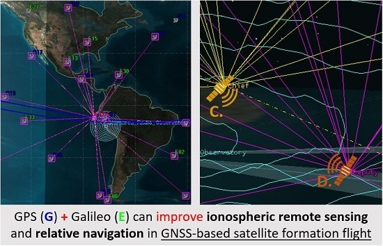
When a formation of two small satellites with on-board GNSS receivers fly through this ESF region, TEC and S4 between the GNSS constellation(s) and the two spacecraft can be measured. This scenario is illustrated in Figure 3. If the dual spacecraft are flying in proximity at different altitudes, the vertical Ne in between can be estimated by dividing the vertical TEC difference from the vertical separation. Compared to some single satellite missions (e.g., LEO GNSS tomography, radio occultation) or ground based remote sensing techniques, this LEO formation flight concept is more advantageous to observing the global and microscale morphology (e.g., precise structure and location) of irregularities that potentially induce GNSS scintillations. Also, ionospheric disturbances associated with Tsunamis or earthquakes can potentially be detected using such a multi-point ionospheric measurement technique, which is applicable to natural hazard monitoring or prediction. The vertical boundaries of irregularities can be estimated by examining the TEC, Ne, and S4, and the horizontal boundaries can be estimated by analyzing the TEC gradients and S4. To cater the observation needs for this scenario, a low inclination (∼10°) orbit was selected to continuously monitor the equatorial region. A small-eccentricity (0.044) orbit is considered to have both spacecraft altitudes vary with time. The initial orbit states of the chief and deputy spacecraft are listed in Table 1. A constant in-track offset of 15 km and radial offset of 1 km was predetermined as the default desired relative orbit configuration during formation keeping, however, elliptic natural orbits should be implemented in the future for a better fuel budget.
An HIL simulation of this ESF scenario was run using the VTFFTB 2.0. The history of relative orbit (radial and in-track) and thrust (radial, in-track, and cross-track) in the Hill’s frame are presented in Figure 4. As shown in Figure 4a, it took 125 s to reach formation keeping in the radial direction (offset within ±2 m); and it took 60 s for the in-track relative distance to reach less than ±2 m offset in Figure 4b. As shown in Figure 4c, thrust in radial and in-track directions were “on duty” to perform formation acquisition (correct the relative orbit from the initial state into the desired state). The first available EKF-based estimation was available at 276 s, where the EKF initialization led to a transient orbit deviation and redundant thrust as well. The filter converged quickly after that, therefore, inconsequential thrust transients are observed for the rest of the simulation. When the satellite fleet entered the ionospheric irregularity (ESF) region around 2200 s, scintillation impacted the navigation performance and disturbed the relative orbit. Throughout this one hour HIL simulation with a maximum thrust limit () of 0.5 m/s, the total thrust used in radial, in-track, and cross-track directions are 22.4665 m/s, 7.6677 m/s, and 1.1758 m/s, respectively.
3.2. Gaileo TEC and Ne Measurements
When the chief satellite soars higher than the deputy satellite, the vertical Ne between the two satellites retrieved from a specific PRN can be computed by the following formula:
where VTEC is the vertical TEC measured by the chief satellite GNSS receiver from a PRN, VTEC is the vertical TEC measured by the deputy satellite GNSS receiver from the same PRN, and ∆h is the height difference between the chief and deputy. Using this method, space-born GNSS receivers can be utilized to retrieve localized Ne given a formation flying orbit with non-zero radial offset. If the measurement accuracy is comparable to or outperforms other measurement techniques (e.g., in-situ Langmuir probe or radio-occultation), the design of a satellite mission (e.g., cost, size, and power budget) can be significantly reduced while the same Ne product can still be generated.
The vertical Ne retrieved from Galileo PRN 30 is plotted against the central height between the two LEO satellites as shown in Figure 5. The TEC result using the E1 and E5a frequency combination is plotted on the left (a), while the result from the E1 and E5b frequency combination is plotted on the right (b). The SR Ne profile is plotted in red, and the measurements using Equation (2) are plotted in blue. Note that, these are not localized (same latitude and longitude) vertical Ne profiles but a vertical projection of the three-dimensional trace of the sounding rocket vertical Ne. Due to a high frequency scattering effect from the raw signals, a low pass filter (critical frequency = 0.01 Hz) is applied to process the raw measurements and the filtered results are plotted in black. After filtering, the Ne measurement results from the HIL simulation become much more consistent with the SR model. In Figure 5b, the measurement results above 500 km are relatively deviated from the model. This is due to the inaccurate DCB estimation with respect to PRN 30 of the E1 and E5b frequency combination. Further analysis indicates the scattering features of the Ne raw measurement is a heritage from TEC, which is associated with the particular receiver model and frequency combination of a specific GNSS constellation. For the NovAtel OEM628 receiver, GPS L2P and L2C tracking is aided by GPS L1. While Galileo E5a, E5b, and E5 AltBOC tracking is unaided, as is GPS L5. The unaided carrier-phase TEC combinations (e.g., E1 and E5a and E1 and E5b) are noisier than the aided ones (e.g., L1 and L2). Therefore, the vertical Ne retrieved using GPS L1 and L2 TEC by the OEM628 receiver is less fluctuated than the vertical Ne retrieved by Galileo (E1 and E5a or E1 and E5b) TEC in the baseline ESF scenario.
3.3. Multi-Constellation Data Fusion
An accuracy improvement on Ne retrieval is found by combining both GPS and Galileo measurements. As shown in Figure 6a, the Ne retrieved from selected GPS (L1 and L2) is combined with the Galileo (E1 and E5b) Ne from a simulation using the 13 July 2018 almanac, when there were 13 operational Galileo satellites. After taking an average of those selected GPS and Galileo PRNs (with outlier-free Ne measurements), a 0.01 Hz low pass filter was applied to plot the final values in black. The SR Ne profile is plotted in red to represent the “true” values. The measurement errors (discrepancy between filtered Ne and “true” value) are plotted in green. It is found that the mean and standard deviation of measurement errors were decreased by 32.83% and 46.12%, respectively, compared to just using the GPS constellation in this simulated scenario.
As expected, an accuracy improvement can also be seen by simulating the GPS and Galileo almanac in a more recent time. As shown in Figure 6b, the Ne retrieved from selected GPS (L1 and L2) is combined with the Galileo (E1 and E5b) Ne from a simulation using a more recent 8 March 2019 almanac, where there were 22 operational Galileo satellites. It is found that the mean and standard deviation of measurement errors were decreased further by 43.34% and 49.92%, respectively, compared to using only the GPS data in the simulated scenario. This accuracy improvement is consistent with the growing number of Galileo satellites and indicates a benefit of applying multi-constellation GNSS SFF for ionospheric remote sensing. Adding a new constellation can improve the geometry and increase the number of line-of-sight measurements, which is beneficial to smooth out the bias in each measurement.
Wavenumber spectra of the Ne measurements were generated to analyze the retrieval resolution on multiple spatial scales of ionospheric plasma structure, based on the 8 March 2019 Almanac and the SR Ne profile. As shown in Figure 7, the wavenumber spectrum of the SR Ne model is plotted in red, the wavenumber spectrum of Ne measurements using L1 and L2 TEC from all visible GPS satellites is plotted in blue, and the wavenumber spectrum of Ne measurements using TEC from all visible GPS satellites plus eight Galileo satellites is plotted in green. The wavenumber k is a function of spatial scale as k = 2/. Ne(k) is the spatial Fourier transform of the Ne profile. The three plasma bubbles can be clearly seen in the spectra at 0.1 < k < 0.2, which corresponds to 30 km << 60 km. Compared to the blue spectrum, the green spectrum is closer to the red spectrum across the whole spatial range except a noisy spike near k = 6. This, once again, demonstrates an improvement of ionospheric electron density retrieval resolution using more satellites from multi-constellation GNSS.
3.4. Formation Configuration Sensitivity Study
A sensitivity study was undertaken to investigate the impact of the variation of the LEO satellite radial offset on the vertical Ne measurements. Based on the 8 March 2019 almanac, three formation flying configurations were simulated respectively with different radial separations during formation keeping: (i) 100 m, (ii) 1000 m, and (iii) 3000 m. The Ne retrieval using Galileo PRN 1 and the E1 and E5b TEC are compared between the three configurations.
By simulating configuration (i) with a radial offset of 100 m in the ESF scenario, very noisy Ne measurements are obtained as shown in Figure 8i. The measurement errors (in green) were computed by differencing the SR modeled Ne (in red) and raw measured Ne (in blue). The average absolute error is cm−3, and standard deviation of errors is cm−3. The raw Ne measurements here are too noisy to distinguish the three plasma bubbles (located approximately at 340–380 km, 395–435 km, and 480–520 km, respectively). The main reason causing such scattering features is the relatively short altitude separation (∼100 m) between the LEO satellites. The VTEC measured at each altitude contains a certain amount of noise and such TEC noise levels are comparable to the real TEC difference between 100 m. Therefore, 100-meter radial separation is not large enough to resolve the E1 and E5b TEC noise from the OEM628 receiver.
By simulating configuration (ii) with a radial offset of 1000 m in the ESF scenario, Ne measurements with a limited amount of noise are retrieved as shown in Figure 8ii. This is the same formation configuration implemented in Section 3.2 and Section 3.3. The average absolute error is cm−3, and standard deviation of error is cm−3. The raw Ne measurements look much better than the result of configuration (a), however, applying a low pass filter can further smooth the results and help visualize the plasma bubbles as demonstrated in the earlier two subsections. By simulating configuration (iii) with a radial offset of 3000 m in the ESF scenario, Ne measurements are retrieved without the data scattering as shown in Figure 8iii. The average absolute error is cm−3, and standard deviation of error is cm−3. The raw Ne measurements are “clean” enough to distinguish the three plasma bubbles without further applying filtering.
A wavenumber spectrum analysis was performed to compare the resolution results between the three different configurations. As shown in Figure 9, the wavenumber spectra of Ne retrieval and SR model are plotted together to determine the multi-scale resolution using each formation configuration in this scenario. Clearly, the 100-m case exhibit the worst performance across the whole spatial range. The 1-km and 3-km cases show comparable agreements with the spectrum of SR Ne model. The agreement for the 1-km case outperforms the 3-km case for smaller scales (k > 1), vice versa.
The two GNSS receivers vertically separated by 3000 m in LEO allows a near optimal Ne retrieval for the larger scale plasma bubbles using Galileo TEC, however, this will decrease the resolution of GPS Ne retrieval because the GPS’s TEC noise level is lower than Galileo’s. Therefore, the 1000 m radial separation was chosen due to a (measurement noise) trade-off between the GPS and Galileo given the OEM628 receiver. The results indicate there is an optimal range of vertical separation (between the satellites in formation) to resolve the spatial scale of a specific ionospheric structure. In future mission designs, the VTFFTB can offer a HIL simulation testbed to determine an optimal geometry of formation flight for ionospheric remote sensing with respect to specific GNSS receivers.
3.5. C/N Level Sensitivity Study
Another sensitivity study was conducted to investigate the impact of the GNSS signal C/N level on the vertical Ne measurements. The GNSS antenna gain for the incoming signals to the receiver on a small satellite can be unstable or below the anticipated level in some scenarios, such as, satellite attitude control error or failure, spacecraft (power system) in a low power mode, and degraded satellite antenna. Any anisotropy in the GNSS antenna gain will imply the tracking PRN C/N will be different because the GNSS satellite signals come from different directions with different relative distances. Also, the power levels of GNSS signals transmitted by different GNSS constellations or different frequency bands from the same constellation are different. Moreover, ionospheric scintillations can impact the C/N level as well. Therefore, it is important to characterize the effect of C/N level on vertical Ne retrieval.
By adjusting the global power level offset in the GNSS simulator, different C/N level tracked by the receiver can be effectively simulated with the isolation of other controlled variables. The result in Figure 8ii is chosen as the reference (power level). Two scenarios of global power offset (applied to all PRNs) on the deputy satellite’s antenna were simulated: (a) −3 dB and (b) −8 dB. The HIL simulation comparison used the default formation configuration based on the 8 March 2019 almanac.
The simulation results show that the lower the C/N is, the more the TEC measurement fluctuates. As a result, more measurement noise is introduced into the vertical Ne retrieval. Figure 10a shows the vertical Ne retrieval for PRN 1 using Galileo E1andE5b TEC with a power offset of −3 dB, where the average absolute error is cm−3 and the standard deviation of error is cm−3. Figure 10b shows the same vertical Ne retrieval except with a power offset of −8 dB, where the average absolute error is cm−3 and the standard deviation of errors is cm−3. By comparing to the reference result in Figure 8ii, the absolute mean and standard deviation of Ne measurement errors becomes larger when the signal power (C/N) decreases.
A comparison using the GPS constellation indicates a similar trend of decreasing accuracy that is in line with the Galileo comparison described above. Choosing the vertical Ne retrieval results using GPS L1 and L2 TEC from PRN 7, the absolute mean and standard deviation of raw measurement errors for the reference power level scenario are cm−3 and cm−3, respectively. For the −3 dB power offset scenario, the absolute mean and standard deviation of Ne measurement errors increase to cm−3 and cm−3, respectively. For the −8 dB power offset case, the absolute mean and standard deviation of measurement errors further increase to cm−3 and cm−3, respectively.
This sensitivity study demonstrates a correlation between the C/N level and the vertical Ne retrieval characteristics: When the C/N is reduced, the Ne retrieval accuracy is reduced and associated with more scattering in the Ne measurements. During the antenna selection process for a LEO satellite with a GNSS receiver, a link budget calculation including the C/N is important in characterizing the ionospheric remote sensing capability.
3.6. Galileo Scintillation Measurements
Other than TEC and electron density, adding the Galileo system will produce more types of GNSS scintillation observations (e.g., different line-of-sights, frequency bands, signal power levels, and modulation schemes), which has advantages for multi-scale ionospheric remote sensing investigations. Several Galileo scintillation observations from a multi-constellation HIL simulation of the baseline ESF scenario based on the 13 July 2018 almanac are demonstrated here. Figure 11a–c present the vertical distribution of Galileo E1, E5a, and E5b effective 1-Hz S4 observed by the chief satellite receiver from all eight visible PRNs. Figure 12a–c show the horizontal view of Galileo E1, E5a, and E5b effective S4 level observed by the chief receiver following the satellite ground track, as the “snapshots” of 1-Hz S4 taken every minute from eight different visible PRNs. Similar observations from the deputy receiver of the fleet (not shown) can be obtained with similar macroscale behavior as the chief. In total, 10 Galileo PRNs were tracked by the deputy LEO receiver during the 1 h ESF scenario. Since the amplitude scintillation modeled in the GNSS simulator is confined in a cuboid region, the high S4 observations from Galileo mostly occur in the corresponding region (290–350 km, 20-21 LT, 0–10°S) near the JRO as anticipated. Therefore, the observation of S4 by SFF can potentially be designed as a tracer or new indicator of ionospheric irregularities.
Because the GNSS simulator currently is only capable of modeling a simplified ionosphere, the amplitude scintillation affects all frequency bands of Galileo and GPS similarly. A multi-constellation, multi-frequency software GNSS receiver was developed and applied to ground-based ionospheric scintillation studies by [28]. Reference [29] utilized a ground-based, multi-constellation, multi-band GNSS data collection system to observe equatorial scintillation. Reference [30] analyzed the multi-frequency responses of GNSS receivers to ionospheric scintillations and characterized the difference in receiver behavior under scintillations across multiple frequency bands. This is currently an important area of investigation and, therefore, space-based, multi-constellation, multi-frequency-band GNSS scintillation measurements will facilitate studying multi-scale ionospheric irregularity impacts on GNSS signals from the perspective of different constellations, frequency bands, modulation schemes, chipping rates, powers, etc. [31].
3.7. Relative Navigation Improvement
The relative navigation robustness is very important when an SFF mission rigorously demands the separation accuracy among their distributed space systems. For instance, the precision of formation keep and relative state estimation for a 1000-m baseline SFF mission is sensitive to the spatial resolution of small-scale (e.g., ≤100 m) ionospheric irregularity or large-scale ionospheric morphology (e.g., size or boundary of plasma structure) observations.
Besides ionospheric remote sensing, the new version of VTFFTB after incorporating Galileo also shows an improvement on relative state estimation. The baseline ESF scenario described in Section 3.1 is used for HIL simulations, in order to compare the EKF-based relative state estimations between a GPS scenario and a multi-constellation scenario. A number of qualitative comparisons were performed, and one comparison based on the 8 March 2019 almanac is shown here as an example. The relative state estimation errors presented in Table 2 are based on a simulation using the GPS (L1) constellation only for relative navigation. The relative state estimation errors in Table 3 is based on a simulation using both the GPS (L1) and Galileo (E1) constellations. The error is defined as the difference between the EKF estimated value and the simulator recorded “truth” after each simulation, and it is calculated including the initialization period before the EKF converges. All the error values in Table 2 and Table 3 are rounded to three decimal places. Note that, the scintillation effect is not fully simulated and the induced cycle slips were not fully addressed in the HIL simulation for simplicity. This is likely the main factor degrading the overall relative estimation performance. However, several non-control simulations on the VTFFTB with more robust algorithms (to handle cycle slips) were used for formation flying relative navigation and their relative position errors were less than 10-cm after the EKF converges. Table 4 gives the computed error decrease percentages of Table 3 relative to Table 2, which quantifies how much relative state estimate errors were decreased by using multi-constellation GNSS (GPS L1 and Galileo E1) against using GPS only. The positive values indicate error decrease, while a negative value indicates an error increase. After a large ensemble of simulations, it is found that the average absolute errors in all ECEF (Earth-centered, Earth-fixed) components of relative position and relative velocity typically decreased. The standard deviation of errors decreased in most cases as well. The simulations based on a newer almanac usually showed better improvement as well due to a larger number of Galileo satellites. Also, the EKF-based relative estimation converge time is typically faster using multi-constellation, compared to using GPS-only. Therefore, relative navigation with both GPS and Galileo constellations can offer better estimation performance, as the dimension of differential GNSS measurement matrix becomes larger with more PRNs.
4. Conclusions
The GPS-based VTFFTB has been successfully upgraded into a multi-GNSS (GPS + Galileo) version. By running HIL simulations of a baseline ESF scenario, the ionospheric remote sensing and EKF estimation capabilities were found to be improved with the addition of Galileo. By comparing to just using the GPS constellation for ionospheric sounding, using GPS (L1, L2) and Galileo (E1, E5b) together decreased the mean and standard deviation of vertical Ne retrieval errors by 32.83% and 46.12% when simulating the 13 July 2018 almanac. A more recent simulation of the 8 March 2019 almanac shows the mean and standard deviation of vertical Ne retrieval errors were decreased further by 43.34% and 49.92% when multi-constellation (GPS and Galileo) data were utilized instead of implementing GPS-only. Using the NovAtel OEM628 receiver, vertical Ne retrieved by the Galileo constellation using E1 and E5a or E1 and E5b TEC are nosier than the Ne retrieved by the GPS constellation using L1 and L2 TEC. The characteristics of retrieved vertical Ne are sensitive to the altitude separation between the two satellites in formation, and level. Sufficiently small altitude separation increases measurement noise, while sufficiently large altitude separation reduces spatial resolution. Lower level decreases the vertical Ne retrieval accuracy and increases the measurement variance. Ionospheric scintillations from more frequency bands, different power levels and modulation schemes can be observed with the new Galileo system. This offers more opportunities for future GNSS-based SFF missions to detect multi-scale ionospheric irregularities. Also, the relative state estimation performance is increased by using both GPS L1 and Galileo E1 data for differential carrier-phase measurement compared to using GPS L1 only.
In order to place onboard GNSS receivers at different altitudes, the formation configurations simulated in the ESF scenario feature a constant radial offset during formation keeping, which is not fuel-efficient especially for small satellite formation flight. Natural relative orbits with bounded motion will be implemented to optimize the fuel budget. To realize an altitude difference between satellites, elliptic or circular relative orbits should be considered and accessed to characterize the Ne retrieval capability while varying the altitude difference between two LEO satellites. Also, the simulation fidelity of the ionosphere requires some improvement to emulate the ionospheric impacts on GNSS signals more realistically. This will facilitate the design and development of new applications to a wider variety of ionospheric phenomena, such as sub-auroral polarization streams (SAPS), polar tongue of ionization, polar cap patches, ULF waves, etc. Last but not least, more GNSS receivers and simulators are being incorporated into the VTFFTB in order to simulate and study multiple-satellite (≥3) real-time formation flight and its applications to multi-scale space weather observation. This will be reported on in the near future.
Author Contributions
Conceptualization, Y.P. and W.A.S.; data curation, Y.P.; formal analysis, Y.P.; funding acquisition, W.A.S.; investigation, Y.P.; methodology, Y.P.; resources, Y.P. and W.A.S.; software, Y.P.; supervision, W.A.S.; validation, Y.P.; visualization, Y.P.; writing—original draft, Y.P.; writing—review and editing, Y.P. and W.A.S.
Funding
The VTFFTB was supported by the AFOSR (Grant # 13-0658-09) and Virginia Tech.
Acknowledgments
The authors would like to appreciate Gregory Earle and Anthea Coster for providing useful suggestions. Also, Y.P. is highly appreciative of receiving the International Association of Geodesy (IAG) Travel Grant to present our work at the 2018 International Workshop on GNSS Ionosphere (IWGI2018) in Shanghai, China.
Conflicts of Interest
The authors declare no conflict of interest.
Abbreviations
The following abbreviations are used in this manuscript:
| VTFFTB | Virginia Tech Formation Flying Testbed |
| HIL | Hardware-in-the-loop |
| SFF | satellite formation flying |
| MMS | Magnetospheric Multiscale |
| GRACE | Gravity Recovery and Climate Experiment |
| ESA | European Space Agency |
| GNC | guidance, navigation, and control |
| PNT | positioning, navigation, and timing |
| GNSS | Global Navigation Satellite System |
| GPS | Global Positioning System |
| LEO | low Earth orbit |
| TEC | total electron content |
| COSMIC | Constellation Observing System for Meteorology, Ionosphere, and Climate |
| CTECS | Compact Total Electron Content Sensor |
| SPORT | Scintillation Prediction Observations Research Task |
| CERTO | Coherent Electromagnetic Radio Tomography |
| ION-F | Ionospheric Observation Nanosatellite Formation |
| NASA | National Aeronautics and Space Administration |
| DRL | German Aerospace Center |
| Ne | electron density |
| RF | radio frequency |
| USB | Universal Serial Bus |
| EKF | Extended Kalman filter |
| HCW | Hill-Clohessy-Wiltshire |
| S4 | amplitude scintillation index |
| VTEC | vertical TEC |
| DCB | Differential Code Bias |
| COTS | commercial off-the-shell |
| ESF | Equatorial Spread F |
| SR | sounding rocket |
| LT | local time |
| JRO | Jicamarca Radio Observatory |
| ECEF | Earth-centered, Earth-fixed |
| SAPS | Sub-Auroral Polarization Streams |
References
- Lissaman, P.; Shollenberger, C.A. Formation flight of birds. Science 1970, 168, 1003–1005. [Google Scholar] [CrossRef] [PubMed]
- Curtis, S. The Magnetospheric Multiscale Mission: Resolving Fundamental Processes in Space Plasmas: Report of the NASA Science and Technology Definition Team for the Magnetospheric Multiscale (MMS) Mission; National Aeronautics and Space Administration, Goddard Space Flight Center: Greenbelt, MD, USA, 1999.
- Tapley, B.D.; Bettadpur, S.; Ries, J.C.; Thompson, P.F.; Watkins, M.M. GRACE measurements of mass variability in the Earth system. Science 2004, 305, 503–505. [Google Scholar] [CrossRef] [PubMed]
- Friis-Christensen, E.; Lühr, H.; Knudsen, D.; Haagmans, R. Swarm—An Earth observation mission investigating geospace. Adv. Space Res. 2008, 41, 210–216. [Google Scholar] [CrossRef]
- Busse, F.D.; How, J.P.; Simpson, J. Demonstration of Adaptive Extended Kalman Filter for Low-Earth-Orbit Formation Estimation Using CDGPS. Navigation 2003, 50, 79–93. [Google Scholar] [CrossRef]
- Mohiuddin, S.; Psiaki, M. Satellite relative navigation using carrier-phase differential GPS with integer ambiguities. In Proceedings of the AIAA Guidance, Navigation, and Control Conference and Exhibit, San Francisco, CA, USA, 15–18 August 2005; p. 6054. [Google Scholar]
- Vierinen, J.; Coster, A.J.; Rideout, W.C.; Erickson, P.J.; Norberg, J. Statistical framework for estimating GNSS bias. Atmos. Meas. Tech. 2016, 9, 1303–1312. [Google Scholar] [CrossRef]
- Anthes, R.A.; Bernhardt, P.; Chen, Y.; Cucurull, L.; Dymond, K.; Ector, D.; Healy, S.; Ho, S.P.; Hunt, D.; Kuo, Y.H.; et al. The COSMIC/FORMOSAT-3 mission: Early results. Bull. Am. Meteorol. Soc. 2008, 89, 313–334. [Google Scholar] [CrossRef]
- Bishop, R.; Hinkley, D.; Stoffel, D.; Ping, D.; Straus, P.; Brubaker, T. First results from the GPS compact total electron content sensor (CTECS) on the PSSCT-2 nanosat. In Proceedings of the AIAA/Utah State University Conference on Small Satellites, Logan, UT, USA, 13–16 August 2012. [Google Scholar]
- Spann, J.; Swenson, C.; Durao, O.; Loures, L.; Heelis, R.; Bishop, R.; Le, G.; Abdu, M.; Krause, L.; Fry, C.; et al. The scintillation prediction observations research task (SPORT): an international science mission using a cubesat. In Proceedings of the AIAA/Utah State University Conference on Small Satellites, Logan, UT, USA, 5–10 August 2017. [Google Scholar]
- Bernhardt, P.A.; Siefring, C.L. New satellite-based systems for ionospheric tomography and scintillation region imaging. Radio Sci. 2006, 41. [Google Scholar] [CrossRef]
- Hall, C.; Davis, N.; DeLaRee, J.; Scales, W.; Stutzman, W. Virginia Tech Ionospheric Scintillation Measurement Mission. In Proceedings of the AIAA/Utah State University Conference on Small Satellites, Logan, UT, USA, 23–26 August 1999. [Google Scholar]
- Leitner, J. A hardware-in-the-loop testbed for spacecraft formation flying applications. In Proceedings of the IEEE Aerospace Conference Proceedings, Big Sky, MT, USA, 10–17 March 2001; Volume 2, pp. 2–615. [Google Scholar]
- Gill, E.; Naasz, B.; Ebinuma, T. First results from a hardware-in-the-loop demonstration of closed-loop autonomous formation flying. In Proceedings of the 26th Annual AAS Guidance and Control Conference, Breckenridge, CO, USA, 5–9 February 2003. [Google Scholar]
- Giralo, V.; D’Amico, S. Distributed Multi-GNSS Timing and Localization for Nanosatellites. In Proceedings of the ION GNSS+, Miami, FL, USA, 24–28 September 2018; pp. 2518–2534. [Google Scholar]
- Eyer, J. A Dynamics and Control Algorithm for Low Earth Orbit Precision Formation Flying Satellites. Ph.D. Thesis, University of Toronto, Toronto, ON, Canada, 2009. [Google Scholar]
- Park, J.I.; Park, H.E.; Park, S.Y.; Choi, K.H. Hardware-in-the-loop simulations of GPS-based navigation and control for satellite formation flying. Adv. Space Res. 2010, 46, 1451–1465. [Google Scholar] [CrossRef]
- Peng, Y.; Scales, W.; Edwards, T.R. GPS-based Spacecraft Formation Flying Simulation and Applications to Ionospheric Remote Sensing. In Proceedings of the ION GNSS+, Miami, FL, USA, 24–28 September 2018; pp. 2804–2818. [Google Scholar]
- Cloutier, J.R. State-dependent Riccati equation techniques: An overview. In Proceedings of the 1997 American Control Conference (Cat. No. 97CH36041), Albuquerque, NM, USA, 6 June 1997; Volume 2, pp. 932–936. [Google Scholar]
- Rideout, W.; Coster, A. Automated GPS processing for global total electron content data. GPS Solut. 2006, 10, 219–228. [Google Scholar] [CrossRef]
- Ouassou, M.; Kristiansen, O.; Gjevestad, J.G.; Jacobsen, K.S.; Andalsvik, Y.L. Estimation of scintillation indices: A novel approach based on local kernel regression methods. Int. J. Navig. Obs. 2016. [Google Scholar] [CrossRef]
- Kelley, M.C. The Earth’s Ionosphere: Plasma Physics and Electrodynamics; Academic Press: Cambridge, MA, USA, 2009; Volume 96, pp. 131–175. [Google Scholar]
- Yeh, K.C.; Liu, C.H. Radio wave scintillations in the ionosphere. Proc. IEEE 1982, 70, 324–360. [Google Scholar]
- Kintner, P.M.; Ledvina, B.M. The ionosphere, radio navigation, and global navigation satellite systems. Adv. Space Res. 2005, 35, 788–811. [Google Scholar] [CrossRef]
- Rodrigues, F.; De Paula, E.; Abdu, M.; Jardim, A.; Iyer, K.; Kintner, P.; Hysell, D. Equatorial spread F irregularity characteristics over Sao Luis, Brazil, using VHF radar and GPS scintillation techniques. Radio Sci. 2004, 39. [Google Scholar] [CrossRef]
- Rino, C.; Tsunoda, R.; Petriceks, J.; Livingston, R.; Kelley, M.; Baker, K. Simultaneous rocket-borne beacon and in situ measurements of equatorial spread F—Intermediate wavelength results. J. Geophys. Res. Space Phys. 1981, 86, 2411–2420. [Google Scholar] [CrossRef]
- Dautermann, T.; Sgammini, M.; Pullen, S. Ionospheric threat simulation for GNSS using the Spirent hardware signal simulator. GPS Solut. 2014, 18, 365–373. [Google Scholar] [CrossRef]
- Peng, S. A Multi-Constellation Multi-Frequency GNSS Software Receiver Design for Ionosphere Scintillation Studies. Ph.D. Thesis, Faculty of theVirginia Polytechnic Institute and State University, Blacksburg, VA, USA, 27 July 2012. [Google Scholar]
- Morton, Y.; Bourne, H.; Carroll, M.; Jiao, Y.; Kassabian, N.; Taylor, S.; Wang, J.; Xu, D.; Yin, H. Multi-constellation GNSS observations of equatorial ionospheric scintillation. In Proceedings of the 2014 XXXI URSI General Assembly and Scientific Symposium (URSI GASS), Beijing, China, 16–23 August 2014; pp. 1–4. [Google Scholar]
- Morton, Y.; Jiao, Y.; van Graas, F.; Vinande, E.; Pujara, N. Analysis of receiver multi-frequency response to ionospheric scintillation in Ascension Island, Hong Kong, and Singapore. In Proceedings of the ION PNT, Honolulu, HI, USA, 20–23 April 2015; pp. 20–23. [Google Scholar]
- Shanmugam, S.; Jones, J.; MacAulay, A.; Van Dierendonck, A. Evolution to modernized GNSS ionoshperic scintillation and TEC monitoring. In Proceedings of the 2012 IEEE/ION Position, Location and Navigation Symposium, Myrtle Beach, SC, USA, 23–26 April 2012; pp. 265–273. [Google Scholar]
Figure 1.
Overall configuration of the multi-constellation version of the Virginia Tech Formation Flying Testbed (VTFFTB).
Figure 1.
Overall configuration of the multi-constellation version of the Virginia Tech Formation Flying Testbed (VTFFTB).

Figure 2.
Total electron content (TEC) processing algorithm flowchart.

Figure 3.
Illustration of the Equatorial Spread F (ESF) scenario.

Figure 4.
Hardware-in-the-loop (HIL) simulation results of the ESF scenario: (a) radial distance history; (b) in-track distance history; (c) thrust history.
Figure 4.
Hardware-in-the-loop (HIL) simulation results of the ESF scenario: (a) radial distance history; (b) in-track distance history; (c) thrust history.

Figure 5.
Vertical Ne retrieved from Galileo PRN 30 TEC: (a) E1 and E5a TEC (b) E1 and E5b TEC.

Figure 6.
Vertical Ne retrieved from selected GPS (L1 and L2) plus Galileo (E1 and E5b) PRNs: (a) 13 July 2018 almanac (b) 8 March 2019 almanac.
Figure 6.
Vertical Ne retrieved from selected GPS (L1 and L2) plus Galileo (E1 and E5b) PRNs: (a) 13 July 2018 almanac (b) 8 March 2019 almanac.

Figure 7.
Wavenumber spectrum comparison between GPS-only and multi-constellation global navigation satellite system (GNSS).
Figure 7.
Wavenumber spectrum comparison between GPS-only and multi-constellation global navigation satellite system (GNSS).

Figure 8.
Vertical Ne retrieval from Galileo PRN 1 with different radial offsets: (i) 100-m; (ii) 1-km; (iii) 3-km.
Figure 8.
Vertical Ne retrieval from Galileo PRN 1 with different radial offsets: (i) 100-m; (ii) 1-km; (iii) 3-km.

Figure 9.
Wavenumber spectrum comparison between different vertical separations.

Figure 10.
Vertical Ne retrieval for PRN 1 using Galileo E1 and E5b TEC with different signal power offsets against Figure 8ii (reference level): (a) −3 dB power offset (b) −8 dB power offset.
Figure 10.
Vertical Ne retrieval for PRN 1 using Galileo E1 and E5b TEC with different signal power offsets against Figure 8ii (reference level): (a) −3 dB power offset (b) −8 dB power offset.

Figure 11.
Vertical distribution of 1-Hz S4 observed from different Galileo frequency bands on the chief’s receiver: (a) Galileo E1; (b) Galileo E5a; (c) Galileo E5b.
Figure 11.
Vertical distribution of 1-Hz S4 observed from different Galileo frequency bands on the chief’s receiver: (a) Galileo E1; (b) Galileo E5a; (c) Galileo E5b.


Figure 12.
Horizontal view of 1-Hz S4 level observed from different Galileo frequency bands on the chief’s receiver: (a) Galileo E1; (b) Galileo E5a; (c) Galileo E5b.
Figure 12.
Horizontal view of 1-Hz S4 level observed from different Galileo frequency bands on the chief’s receiver: (a) Galileo E1; (b) Galileo E5a; (c) Galileo E5b.


Table 1.
Initial orbital states of the satellite fleet.
| Epoch: 2019.03.08 01:00:00.00 (GPS); Week Number: 2043; GPS Seconds of Week: 435600 | ||||
|---|---|---|---|---|
| Orbital Elements | Chief Spacecraft | Deputy Spacecraft | Relative State in Body Frame | |
| Semi-major axis a (m) | 6880540 | 6879040 | Radial offset (m) | |
| Eccentricity e | 0.044 | 0.044 | In-track offset (m) | |
| Inclination i (°) | 10 | 10 | Cross-track offset (m) | |
| Argument of perigee (°) | 180 | 180 | Radial velocity (m/s) | |
| Long. of ascending node (°) | 67.4893 | 67.479 | In-track velocity (m/s) | 1.7605 |
| Mean anomaly M (°) | Cross-track velocity (m/s) | |||
Table 2.
Relative state errors using GPS.
| Component | Average Absolute Error | Standard Deviation of Error |
|---|---|---|
| X (m) | 6.372 | 3.031 |
| Y (m) | 9.373 | 3.393 |
| Z (m) | 2.550 | 0.801 |
| Vx (cm/s) | 0.627 | l1.365 |
| Vy (cm/s) | 0.782 | 1.737 |
| Vz (cm/s) | 0.180 | 0.619 |
Table 3.
Relative state errors using multi-constellation GNSS.
| Component | Average Absolute Error | Standard Deviation of Error |
|---|---|---|
| X (m) | 6.141 | 3.085 |
| Y (m) | 7.399 | 3.000 |
| Z (m) | 2.165 | 0.637 |
| Vx (cm/s) | 0.440 | 1.092 |
| Vy (cm/s) | 0.575 | 1.254 |
| Vz (cm/s) | 0.133 | 0.386 |
Table 4.
Comparison of relative state estimation errors.
| Component | Decrease Percentage of Average Absolute Error | Decrease Percentage of Standard Deviation of Error |
|---|---|---|
| X | 3.63% | −1.78% |
| Y | 21.06% | 11.58% |
| Z | 15.10% | 20.47% |
| Vx | 29.87% | 20.02% |
| Vy | 26.49% | 27.83% |
| Vz | 26.03% | 37.63% |
© 2019 by the authors. Licensee MDPI, Basel, Switzerland. This article is an open access article distributed under the terms and conditions of the Creative Commons Attribution (CC BY) license (http://creativecommons.org/licenses/by/4.0/).
Share and Cite
MDPI and ACS Style
Peng, Y.; Scales, W.A. Satellite Formation Flight Simulation Using Multi-Constellation GNSS and Applications to Ionospheric Remote Sensing. Remote Sens. 2019, 11, 2851. https://doi.org/10.3390/rs11232851
AMA Style
Peng Y, Scales WA. Satellite Formation Flight Simulation Using Multi-Constellation GNSS and Applications to Ionospheric Remote Sensing. Remote Sensing. 2019; 11(23):2851. https://doi.org/10.3390/rs11232851
Chicago/Turabian StylePeng, YuXiang, and Wayne A. Scales. 2019. "Satellite Formation Flight Simulation Using Multi-Constellation GNSS and Applications to Ionospheric Remote Sensing" Remote Sensing 11, no. 23: 2851. https://doi.org/10.3390/rs11232851
Note that from the first issue of 2016, this journal uses article numbers instead of page numbers. See further details here.