Land Surface Phenologies and Seasonalities in the US Prairie Pothole Region Coupling AMSR Passive Microwave Data with the USDA Cropland Data Layer

Abstract

Land surface phenologies and seasonalities in the US Prairie Pothole Region (PPR) were characterized using land surface variables derived from the coarse spatial resolution (25 km) Advanced Microwave Scanning Radiometer (AMSR) blended data for 2003 to 2016 linked with the optically based USDA NASS Crop Data Layer (CDL) at a much finer spatial resolution. Two transects of AMSR pixels—one in east-central North Dakota and the other in eastern South Dakota—were selected for analysis. The AMSR data were grouped earlier (2003–2005, 2007) and later (2013–2016) to emphasize temporal change and to avoid data discontinuity in 2011–2012 and a major drought in 2006. The nonparametric Mann-Kendall trend test on the CDL data revealed that area in grasslands and wetlands strongly decreased in both transects, while corn and soybean coverage strongly increased. In crop-dominated sites, the AMSR vegetation optical depth (VOD) time series caught the early spring growth, ploughing, and crop growth and senescence. In contrast, the VOD time series at grassland dominated sites exhibited a lower peak but extended growth period. Crop-dominated sites had significantly higher amplitude VODs in both periods and transects. Based on the paired two-sample t-test, neither the peak VOD amplitude nor the peak VOD timing measured in accumulated growing degree-days was significantly different between temporal groups in the North Dakota transect. In contrast, in South Dakota, both the peak VOD amplitude and its timing were significantly different with shifts to later peak timing during the 2013–2016 period. In addition, in South Dakota but not North Dakota, there were significantly earlier shifts in the timing of peak growing degree-days and peak precipitation water vapor. Both spatial and temporal changes in AMSR land surface variables are linked to shifts in land cover along the South Dakota transect as revealed in the CDL data. More research is required to understand the dynamics evident in the passive microwave time series.

1. Introduction

The Prairie Pothole Region (PPR) is an important grassland and wetland region in the Northern Great Plains that elongates NW-SE across the Canada-US border. Wetlands in this region are important habitats for migratory waterfowl and other wildlife, supporting more than 50% of North America’s migratory waterfowl. Wetlands in this region also provide multiple ecosystem services.

Grasslands and wetlands in the PPR have been converted to croplands in recent years [1,2,3]. Crops cultivated in the PPR are also changing; traditional areas of spring wheat and alfalfa/hay have been switched over to more profitable corn and soybeans. In this study, cropland is defined as all cultivated crops, other than hay and alfalfa. There are several reasons for the expansion of crops, particularly corn and soybeans, in the PPR. Biofuel demand boomed in the late 2000s [4]. High crop prices and unlimited crop insurance subsidies also play an important role [1,5]. The price of corn and soybeans was more than tripled between 2002–2012 [1]. The development of cold- and drought-tolerant crop varieties also helped the expansion of corn and soybeans to the north and west, pushing the center of the corn belt to the northwest [1,6]. High commodity prices in recent years have increased the opportunity cost of participating in the Conservation Reserve Program (CRP), and program enrollment decreased [7]. The amount of CRP land has steadily declined since 2008, after reaching a peak enrollment in 2007 [8]. Between 2010 and 2013, 30% (more than 530,000 ha) of expiring CRP land parcels were returned to the production of five major crops (corn, soybeans, winter and spring wheat, and sorghum) in the 12-state Midwestern region of the United States that enclosed the ecologically important PPR [8]. Grasslands were the largest type of CRP land converted (360,000 ha), followed by specifically designated wildlife habitat (76,000 ha), and wetland areas (53,000 ha). The aggressive conversion of grasslands to croplands in this biodiversity hub can potentially lead to the deterioration of native species, as reported elsewhere [5,9,10].

The United States Department of Agriculture (USDA) Crop Data Layer (CDL) has been widely used to show land cover dynamics in the PPR. The CDL is a raster-based, georeferenced, and crop/land cover specific classification annual data layer for the conterminous USA [11]. It is mainly derived from optical remote sensing data and has a spatial resolution of 30 m (and 56 m in earlier years). Despite its many advantages, the CDL has limitations including interstate data inconsistencies (CDL data were initially produced for each state independently), varying lengths of the CDL data record between states, and limited geographic coverage (conterminous USA) [12,13,14]. Moreover, optical remote sensing data, upon which the CDL is based, are affected by atmospheric effects and cloud contamination [15,16,17].

Passive microwave data are less sensitive to atmospheric contamination, solar illumination constraints, and cloud effects due to much longer wavelengths and direct primary reliance on terrestrial rather than solar radiation to illuminate the land surface. Due to these characteristics, passive microwave data have a fine temporal resolution that can help to monitor the finer temporal dynamics of land covers. Passive microwave data are directly proportional to dielectric properties of land surface parameters, which in turn are sensitive to the water content of such materials [18,19,20,21]. They are sensitive to soil water content, vegetation water content, and aboveground biomass [16]. Land cover dynamics studies based on satellite microwave data include vegetation phenology assessment [22,23,24,25,26], vegetation drought response [27,28], dryland carbon dynamics [29], and growing season variability [30,31]. The main drawbacks of passive microwave datasets include coarse spatial resolution due to the faint microwave emissions from the land surface [15,32], sensitivity to radio frequency interference (RFI) [33,34], and signal degradation or loss due to snow cover and frozen ground [22,23].

The two main objectives of this research were: (1) to characterize the land surface phenologies and land surface seasonalities in the US PPR by coupling the USDA Crop Data Layer (CDL) with the Advanced Microwave Scanning Radiometer (AMSR) enhanced land surface parameters; and (2) to assess whether the passive microwave AMSR derived metrics are able to detect the conversion of grassland/pasture into croplands within the study region. The findings in this research can improve our understanding of land cover dynamics in this sensitive area and help to inform natural resource managers and decisionmakers. It also can inform the research community about the efficacy and performance of passive microwave data for analyzing land cover dynamics.

2. Study Region, Data, and Methodology

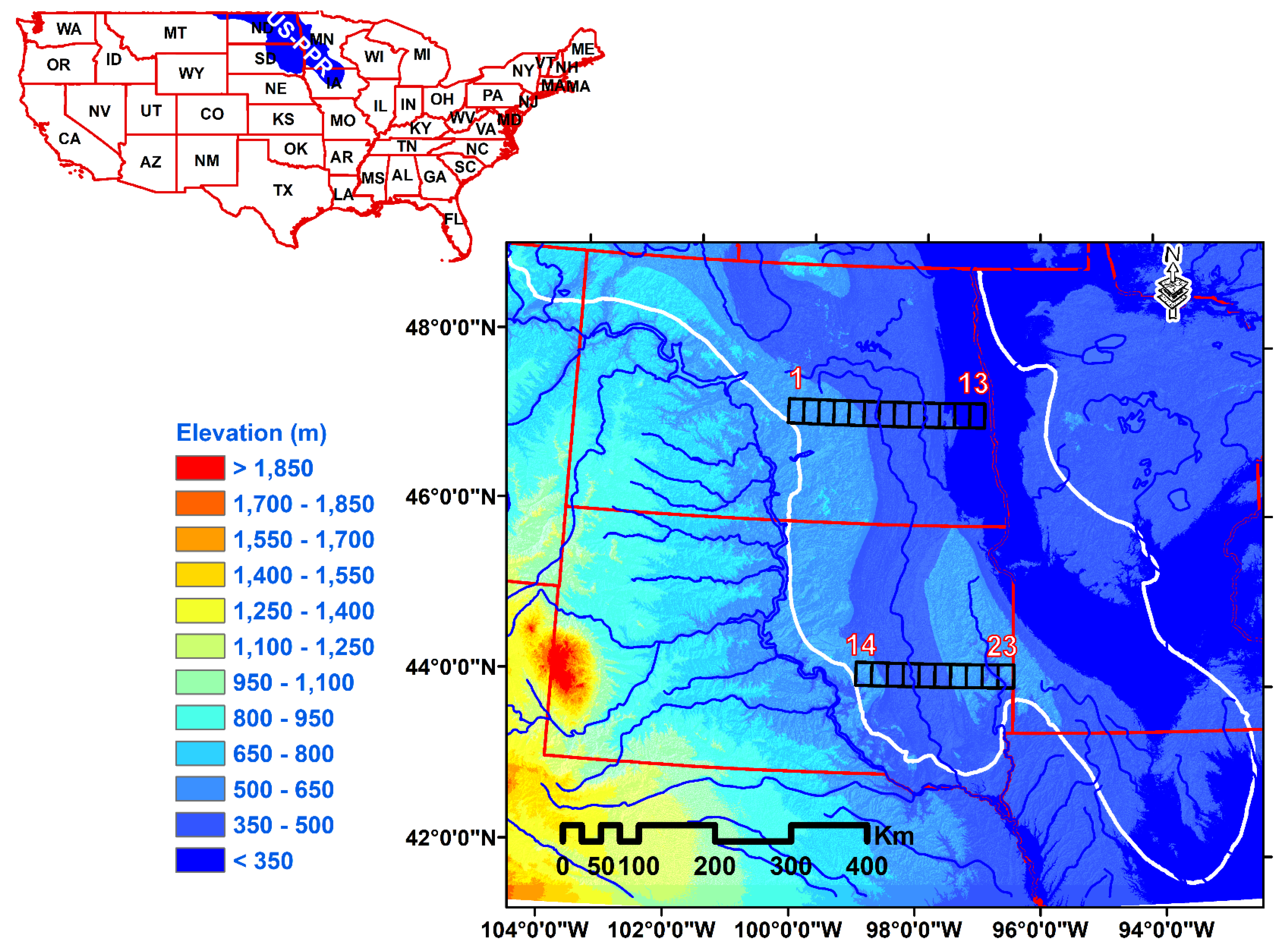
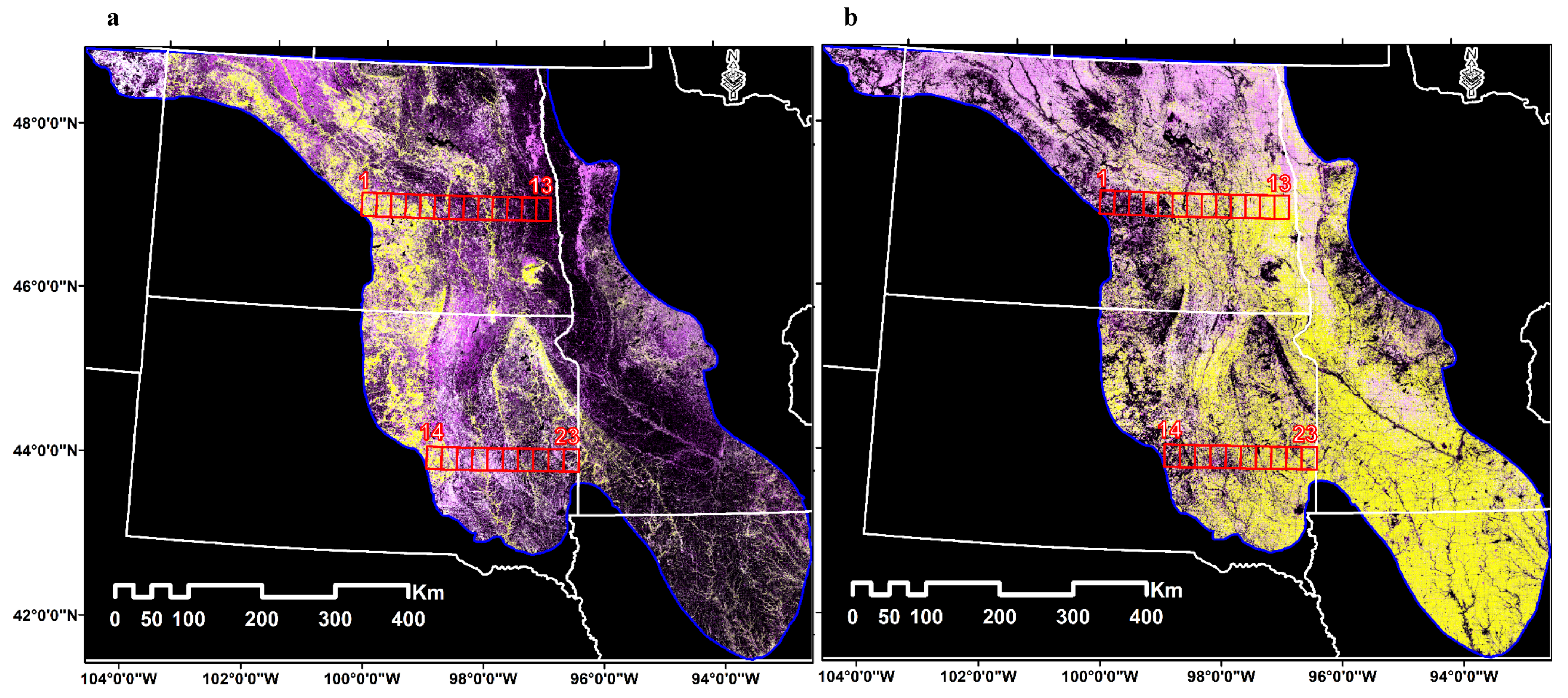
2.1. Study Region

The Prairie Pothole Region (PPR) is an area of midgrass and tallgrass prairie (ecosystems with enormous stretches of flat grassland with moderate temperatures, moderate rainfall, and few trees) that contains thousands of shallow wetlands known as potholes. Elevation in the PPR ranges between 200–800 m above mean sea level (Figure 1) [35].

The persistency maps shown in Figure 2 were based on 11 years (2006–2016) of CDL cropland and grassland time series data. The study period maximum, minimum, and mean percentage for each land cover were calculated. The maximum, mean, and range percentages were displayed in the red, green, and blue color planes respectively [18,36,37,38]. Such combinations result in yellow for temporally stable core areas of the given crop/land cover type in the given period; white for temporally unstable core areas; magenta for unstable peripheral areas; black for non-occurrence of given land cover type during the given study period [18,36,37,38].

The CDL land cover stability maps help us to select AMSR pixel transects that are dominated by grass and crop. For the AMSR data analyses, two transects were selected (black grids in Figure 2), composed of 13 AMSR pixels in east-central North Dakota and 10 pixels in South Dakota. The transects that run from the grassland/pasture dominated west (cf. Figure 2a) to cropland dominated east (cf. Figure 2b).

2.2. Data

Since its beginning in 1997, the USDA NASS Crop Data Layer (CDL) has been developed from farmers reports and satellite datasets, including Landsat TM and ETM+, Indian Remote Sensing Satellite (IRS, RESOURCESAT-1 Advanced Wide Field Sensor (AWiFS)), MODIS, and the National Land Cover Data set (NLCD; [11,39,40]). Within the US PPR, 14 (2003–2016) years of CDL data for the North Dakota transect and 11 (2006–2016) years of CDL data for the South Dakota were used.

The passive microwave global land parameter data record version 2 is a blended dataset of the Advanced Microwave Scanning Radiometer for EOS (AMSR-E; June 2002 to October 2011) on the NASA EOS Aqua satellite and the Advanced Microwave Scanning Radiometer 2 (AMSR2; July 2012 to present) sensor on the JAXA GCOM-W1 satellite [38,41,42]. The blended AMSR-E/AMSR2 dataset includes gap-filled data from a Chinese microwave radiometer that is not directly comparable to the AMSRs so that these data were excluded from our analyses unless otherwise stated. The blended dataset (simply AMSR hereafter) provides twice-daily temporal resolution (1:30 a.m. descending and 1:30 p.m. ascending local equator overpass time) at coarse spatial resolution (25 km). AMSR variables that were used for this study include surface air temperatures (ta), vegetation transmittance (tc), atmospheric precipitable water vapor (V), and fractional open water (fw).

2.3. Methods

Fourteen years (2003–2016) of annual CDL data were used for the North Dakota transect and 11 years (2006–2016) for the South Dakota transect. Six main crop layers (corn, soybean, spring wheat, winter wheat, durum wheat, and sunflower), grasslands, wetlands, alfalfa, and other hay/non-alfalfa were extracted from the CDL.

For each type of crop or land cover, the average percent cover type was calculated within each AMSR pixel of the two study transects. Cover change trends for each cover type were then calculated for each AMSR pixel using the nonparametric Mann–Kendall trend test. The Mann–Kendall trend test detects increasing or decreasing monotonic trends, typically in annual data. The test is not sensitive to data distribution and gives an exact significance level for the detected trend.

Fourteen years (2003–2016) of twice-daily AMSR data were used. An eight-day retrospective moving average smoothing was applied separately to the daytime and nighttime time series to fill data gaps that occurred due to satellite swath width, snow cover, and other factors.

The daytime and nighttime values of each AMSR data variable (V, VOD, and fw, except air temperature) were averaged to get a 24-hour daily value. The daytime and nighttime air temperatures were used to calculate growing degree-days (GDD). GDD is the daily mean temperature increment above a temperature threshold of 0 °C (=273.15 K):

$$GDD=max\left[\frac{t_{ASC}+t_{DES}}{2}-273.15,0\right]$$

(1)

where t_ASC and t_DES are the ascending and descending pass temperatures, which roughly corresponds to the daytime (~13:30) and nighttime (~01:30) temperatures, respectively.

Vegetation Optical Depth (VOD) is a microwave analogue of the NDVI. It is sensitive to crop water content and biomass (Jones et al. 2012). VOD is calculated from vegetation transmittance (tc).

$$VOD={-\log }_{\mathrm{e}}\left(\mathrm{tc}\right)=-\mathrm{LN}\left(\mathrm{tc}\right)$$

(2)

Finally, the growing season data (DOY 91-305, approximating an annual cycle of April through October) were subsetted for the main analysis. This step also avoided the frozen season when no data were available [21]. The AMSR data were divided into two temporal groups (2003–2005 plus 2007, and 2013–2016) to avoid the 2006 drought year and the Chinese Microwave Radiation Imager (MWRI) data spliced to gap fill in 2011 and 2012. The two temporal groups of AMSR data were compared using the pairwise two-sample t-test for means to test for differences indicating possible cover change [43,44].

Accumulated GDD (AGDD) is the simple accumulation of GDD with an annual restart on DOY 91.

$${\mathrm{AGDD}}_t={\mathrm{AGDD}}_{t-1}+{\mathrm{GDD}}_t$$

(3)

A downward-arching Convex Quadratic (CxQ) model was used to characterize the temporal development of VOD, GDD, and V as a function of AGDD:

$$VO{D}_t=\alpha +\beta AGD{D}_t-\gamma AGD{D}_t{}^2$$

(4)

where the intercept α is the background VOD at the start of observation period, the linear parameter β affects the slope, and the quadratic parameter γ controls the curvature. Since the shape of the curve is downward arching, the sign of the β coefficient is positive and the sign of the γ coefficient is negative.

Since full VOD curves were not readily fit for the CxQ model [18], breakpoints of the first derivative (y′) of the VODs and AGDDs were used to find the starting and ending points to improve the CxQ fit.

$$y^{\prime }=\frac{VO{D}_{i+1}-VO{D}_i}{AGD{D}_{i+1}-AGD{D}_i}$$

(5)

where y′ is the first derivative of VOD and AGDD. The CxQ model was then fitted for the VOD time series data using these starting and ending points.

Two metrics were derived from the fitted parameter coefficients for the GDD, V, and VOD time series: (1) peak height (PH); and (2) thermal time to peak (TTP), which is the amount of AGDD required to reach the peak height of GDD or V or VOD.

$$\mathrm{PH}=\alpha -\frac{{\beta }^2}{4\gamma }$$

(6)

$$\mathrm{TTP}=\frac{-\beta }{2\gamma }$$

(7)

where α, β, γ are the fitted parameter coefficients for a particular pixel time series.

3. Results

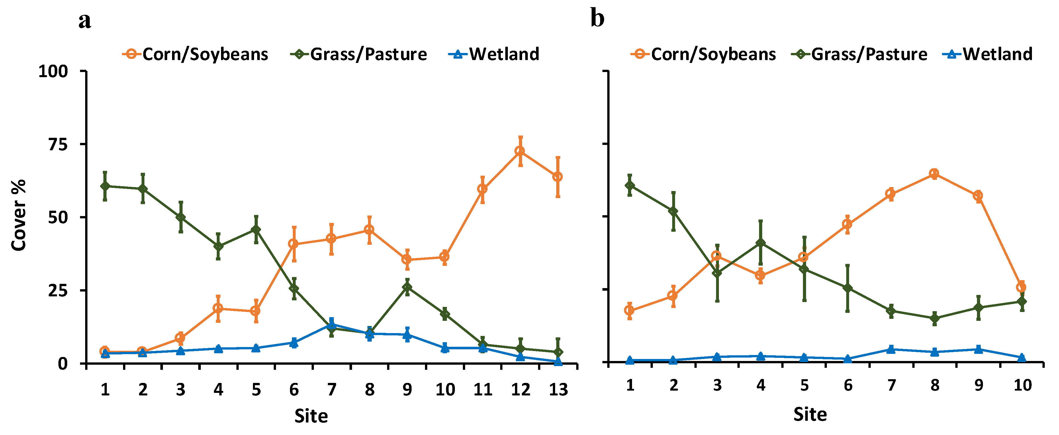
3.1. Mean CDL Land Cover Percentages at AMSR Scale

Aggregated CDL land cover percentages by selected AMSR pixel sites for transects in North Dakota (ND; sites 1–13 in

Table 1. The temporal average proportion of cover type for the 13 AMSR-pixels study sites transect in ND (2003–2016) and 10 sites in SD (2006–2016). Note the general spatial trend of crop versus grassland/pasture covers in both transects.

site	Cover Type (%)
	Grass/Pasture	Corn	Soybean	Sunflower	Durum Wheat	Spring Wheat	Winter Wheat	Alfalfa	Other Hay	Wetlands
North Dakota Sites
1	60.7	1.0	2.8	0.8	0.1	7.6	0.1	0.9	2.5	2.7
2	59.8	1.0	2.9	0.5	0.1	5.6	0.1	1.2	4.7	2.8
3	50.1	1.9	6.6	0.6	0.1	7.9	0.2	1.1	2.3	3.4
4	40.0	4.3	14.5	1.1	0.2	12.2	0.2	0.8	1.5	4.0
5	45.8	4.0	13.9	0.8	0.1	8.1	0.3	1.0	1.8	4.1
6	25.6	12.2	28.7	1.3	0.0	9.0	0.1	1.0	1.0	5.6
7	12.0	9.8	32.7	0.9	0.0	14.4	0.1	0.6	0.5	10.5
8	10.3	11.9	33.7	1.1	0.0	19.1	0.1	0.4	0.3	7.9
9	26.2	9.1	26.4	0.3	0.0	15.2	0.2	1.1	0.5	7.8
10	16.9	16.3	35.7	0.6	0.0	11.2	0.2	1.0	0.4	4.2
11	6.4	22.0	37.4	1.2	0.0	14.2	0.2	0.7	0.1	4.2
12	5.1	30.7	41.9	0.7	0.0	8.1	0.2	0.3	0.1	1.7
13	3.9	17.2	46.6	0.7	0.0	18.4	0.1	0.2	0.1	0.4
South Dakota Sites
14	60.8	11.2	6.4	1.5	0.0	2.8	2.6	1.7	6.2	0.7
15	51.8	13.2	9.4	0.4	0.0	1.5	3.0	1.7	12.1	0.6
16	30.5	20.1	16.3	0.1	0.0	0.7	4.0	2.3	16.5	1.9
17	41.0	17.1	12.6	0.0	0.0	0.4	1.2	4.1	13.9	2.0
18	32.0	17.9	17.8	0.1	0.0	1.6	3.5	2.3	17.6	1.6
19	25.4	23.0	24.2	0.1	0.0	1.3	2.9	2.1	12.8	1.1
20	17.5	28.6	29.0	0.0	0.0	0.4	0.7	1.9	1.9	4.5
21	15.0	33.4	31.2	0.0	0.0	0.4	0.2	2.0	1.2	3.5
22	18.7	31.5	25.4	0.0	0.0	0.7	0.3	2.2	5.4	4.4
23	20.9	37.7	25.4	0.0	0.0	0.9	0.2	2.9	3.2	1.5

, Figure 3a) and in South Dakota (SD; sites 14–23 in Table 1, Figure 3b) showed that western sites in both states/transects were dominated by grasslands/pasture, while eastern sites were dominated by croplands (2003/06–2016 averages). Figure 3 presents the major dynamic covers, namely grassland/pasture and corn plus soybeans, in addition to wetlands. The standard error bars (2SE) indicate that the grassland/pasture in the South Dakota transect mid-sites faced strong interannual variation.

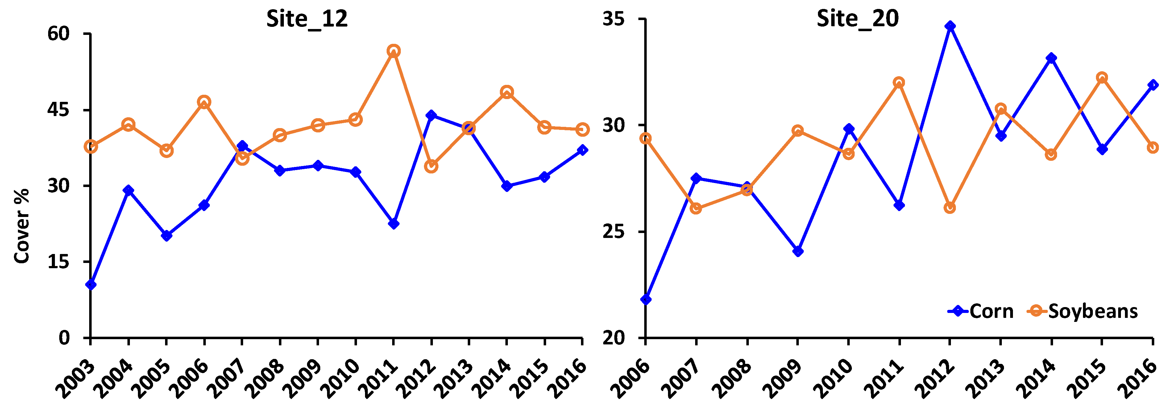
3.2. CDL Land Cover Time Series at the AMSR Pixel Scale

Corn and soybean percentages within a given AMSR pixel (site) alternated from year to year, i.e., when corn cover percentage increased, soybean cover percentage decreased and vice versa, due to crop rotation (Figure 4).

The Mann–Kendall trend analysis (Figure 5) revealed that grassland/pastures, spring wheat, winter wheat, and wetland covers decreased in the study sites between 2003/06 and 2016; while corn, soybeans, and alfalfa/other hay cover increased over the same period and sites. Grassland/pasture cover decreased in all study sites. At ND sites, the decrement was significant only for the eastern half of crop-dominated sites (Figure 5a). The existing small proportions of grassland/pasture on these eastern crop-dominated sites showed strongly conversion to croplands.

In contrast, in SD the grassland/pasture decrement was more pronounced in the western grassland dominated sites (Figure 5b). Wetlands decreased in the eastern half of ND and across all study sites in SD. However, these decrements were significant only at a few study sites. Spring wheat cover decreased at all sites, except the two westernmost grassland dominated sites in ND. The decrements in spring wheat were significant in middle and eastern ND sites. Winter wheat decreased in nearly all study sites. The decrements were significant at all SD sites and at the middle positions along the ND transect. Corn and soybean increased at all sites. These increments were significant at nearly every site. Increment significance levels were more pronounced in the western grassland-dominated sites of both transects, where there are more grasslands available for conversion to croplands. Alfalfa and other hays increased at all sites, but the increments were significant mostly in ND.

3.3. Interannual Dynamics of Land Surface Phenology and Seasonality

The vegetation optical depth (VOD) time series revealed that crop dominated sites (green lines in Figure 6) experienced lower peaks in 2005 in ND. The grassland/pasture covers were stressed by the 2006 drought compared to croplands. The fractional open water (fw) time series (Supplementary Figure S1) revealed that years 2003, 2004, 2006, and 2008 were drier years; whereas, 2007 and 2009 were wetter years. ND sites experienced higher open fractional water compared to SD sites. The AMSR-E & AMSR 2 data gap-filled by the Microwave Radiation Imager (MWRI) onboard the Chinese FengYun 3B (FY3B) satellite data introduced some artifacts in the 2011 and 2012 AMSR product [38]; thus, those data are neither described here nor included in subsequent sections (Figure 6 & Supplementary Figure S1).

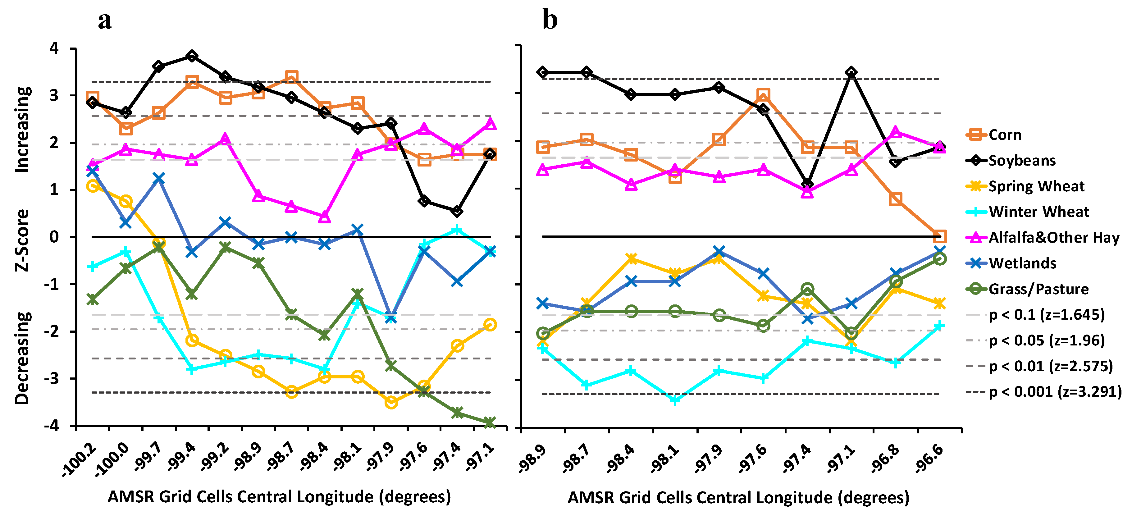
3.4. Spatial Dynamics of Land Surface Phenology

Crop-dominated eastern study sites VOD time series (sites 10–13 and 21–23 caught the early spring weed growth, ploughing, and crop growth dynamics (Figure 7). In contrast, the VOD time series at grass-dominated sites (western sites from 1–3 and 14–16) exhibited a lower but more extended amplitude throughout the non-frozen season. The spatial series of VOD in ND for 2003–2005 plus 2007 shows depressed growth midseason for the sites with mixed to dominant cropland fractions along the transect (sites 5–13). This depressed growth was introduced from the 2005 season of lower VOD (Figure 6a).

Along the ND transect, peak VOD in the eastern sites lags that of the western site’s peak by about two to three weeks (see also Figure 9). In contrast, at the western grassland dominated sites in SD, the VOD peaks about the same time or can even lag those in the eastern crop dominated sites.

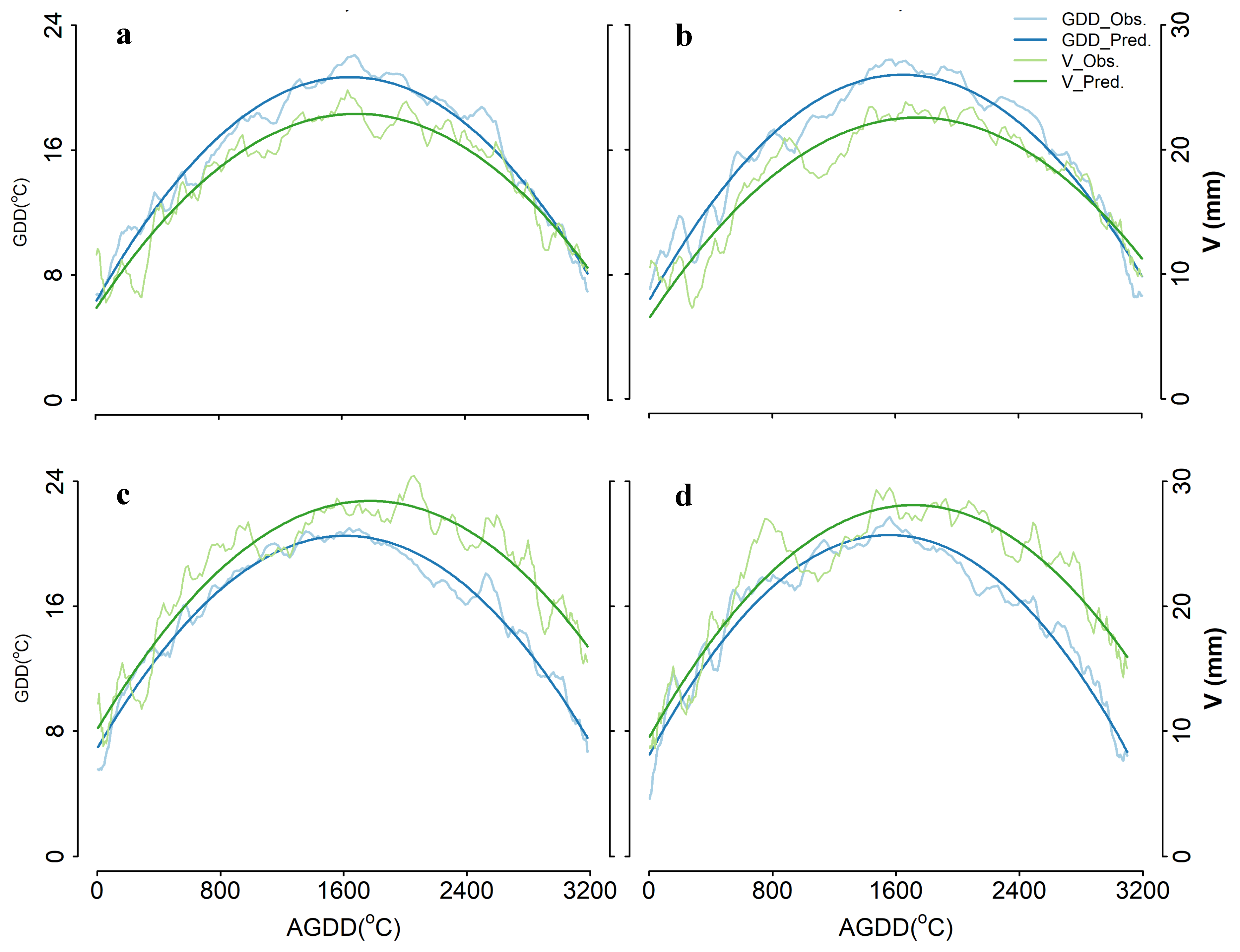
3.5. Convex Quadratic Models for GDD and V

GDD and precipitable water vapor (V) were well fitted with the convex quadratic curves for all sites: for GDD, 0.84 < R² < 0.88; and for V, 0.72 < R² < 0.75. At grassland/pasture dominated sites, the fits for GDD and V were better than at cropland dominated sites (in Figure 8, a,b vs. c,d). GDD appeared to track day-to-day fluctuations of V (Figure 8). However, GDD and V diverge in croplands starting at the earlier peak of GDD (Figure 8c,d). The fits between temporal groups show little difference at either site (Figure 8a vs. Figure 8b and Figure 8c vs. Figure 8d).

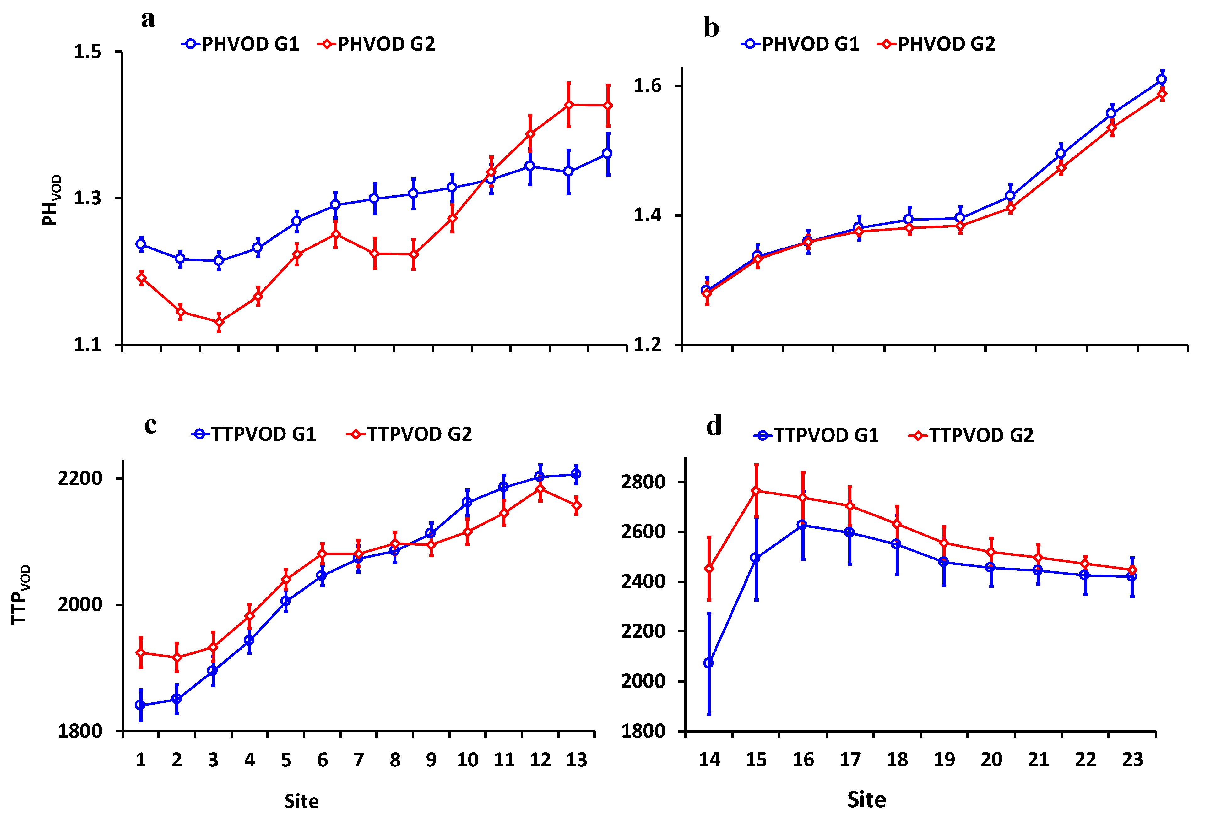
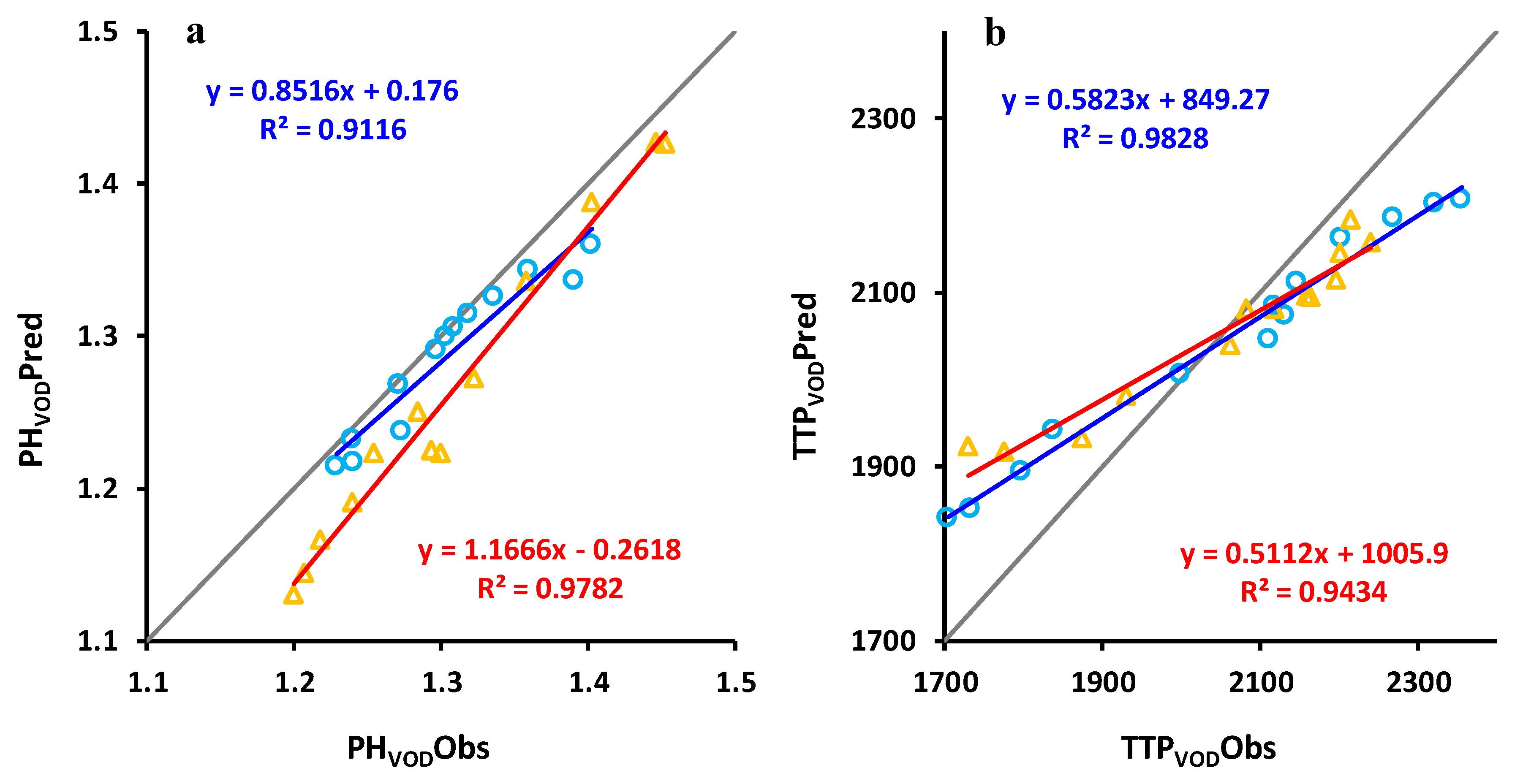
3.6. Spatial and Temporal Variation in Land Surface Phenology and Seasonality Metrics

Crop dominated sites exhibited substantially higher average VOD amplitudes (peak heights) in both temporal groups (2003–2005 plus 2007 and 2013–2016) in both ND (Figure 9a) and SD (Figure 9b). These metrics showed distinct spatial trends. The TTP_VOD at crop dominated sites in ND (Figure 9c) showed large lags (~4 weeks) compared to grassland/pasture dominated sites. For both temporal groups in ND, TTP_VOD displayed a strong spatial trend increasing west to east (Figure 9c). In contrast, TTP_VOD in grassland/pastures dominated sites were generally ahead by 1–2 weeks in SD (Figure 9d) and there was a substantial difference in TTP_VOD in western SD between groups. The difference between grassland/pasture dominated and crop dominated study sites TTP_VOD was larger in the SD transect (800 °C) than in the ND transect (400 °C) (Figure 9c vs. Figure 9d).

Peak Height for GDD (PH_GDD) for both temporal groups lacked distinct patterns in ND (Supplementary Figure S2a), while they were significantly lower for crop dominated sites compared to corresponding grassland/pasture dominated sites in SD (Supplementary Figure S2b). PH_GDD in the SD transect displayed a strong spatial trend corresponding to the transition from grassland/pasture to cropland dominated land cover. Also, in the SD transect, TTP_GDD for grassland/pasture covers lagged TTP_GDD for crop covers (Supplementary Figure S2d). In the ND transect lack, TTP_GDD lacked this clear distinction (Supplementary Figure S2c). Average TTP_GDD during 2013–2016 showed a slight lag (< 100 °C) of grassland/pasture dominated sites relative to crop dominated sites.

Peak values of V (PH_V) in ND were significantly higher for crop dominated sites (Supplementary Figure S2e); whereas, PH_V were significantly lower for crop dominated sites in SD (Supplementary Figure S2f). PH_V in both transects displayed significant spatial trends but in opposite directions: PH_V increased from grassland/pasture to crop dominated sites in ND but decreased in SD. In SD, TTP_V for grassland/pasture dominated sites exhibited a very strong lag (~400 °C) compared to crop dominated sites (Supplementary Figure S2h). There was no clear contrast of TTP_V in ND (Supplementary Figure S2g).

At ND sites TTP_VOD lagged TTP_GDD and TTP_V by ~2.5 to 4.5 weeks and 2.0 to 3.5 weeks, respectively (Figure 9c, Supplementary Figure S2c,g). The lags were two-fold for crop dominated relative to grassland/pasture dominated sites. In SD, these lags ranged 5–6 weeks, and 4.5 to 5.5 respectively, while the lag magnitudes were longer on croplands by about 1 (Figure 9d, Supplementary Figure S2d,h). TTP_GDD and TTP_V occurred at similar times with a slight lag of the TTP_V in both transects (Supplementary Figure S2c,d,g,h).

Based on the paired two-sample t-test of the transect means, the means of PH_VOD from the two temporal groups (g1 is 2003–2005 plus 2007 and g2 is 2013–2016) in the ND transect were not significantly different from each other (Figure 9a,

Table 2. Pairwise two sample t-tests for differences in mean difference (µd) for metrics between two temporal groups (viz., g2–g1, where g1 is 2003–2005 plus 2007 and g2 is 2013–2016). Bold indicates highly significant (p < 0.01) differences.

Transect	stat	PHVOD	TTPVOD	PHGDD	TTPGDD	PHV	TTPV
ND	µd	−0.03	11.19	0.15	−23.96	−0.39	4.80
	p-value	0.14	0.36	<0.01	<0.01	<0.01	0.632
SD	µd	−0.01	122.38	−0.06	−51.68	−0.458	−53.23
	p-value	<0.01	<0.01	<0.01	<0.01	<0.01	<0.01

). Likewise, in ND, there was no significant difference in TTP_VOD between g1 and g2 (Figure 9c, Table 2). In contrast, the PH_VOD and TTP_VOD in SD were significantly different, with PH_VOD being slightly higher in g1 (Figure 9b, Table 2) and TTP_VOD being longer in g2 (Figure 9d, Table 2). PH_GDD, TTP_GDD, and PH_V were all significantly different in ND, but the magnitudes are small (Table 2 and Figure S2a,c,e, respectively). In SD, the temporal pairs for each metric were significantly different, but magnitudes were small except for TTP_VOD where g2 was several days longer in terms of AGDD than g1 (Table 2, Figure 9d).

The CxQ model captured well the PH_VOD for the temporal groups in ND (Figure 10a); whereas, the TTP_VOD were substantially off (Figure 10b) compared to the observed growing season maxima. Predicted TTP_VOD for the grassland/pasture dominated sites substantially leads observed TTP_VOD, but the modeled TTP_VOD lags the observed TTP_VOD in the crop dominated sites. Crops VOD curves ascended smoothly during the first half of the growing season, while it dropped sharply in the second half (Figure 7). Grassland/pasture VOD curves displayed relatively slow and smooth changes throughout the growing period (Figure 7).

4. Discussion

The regional pattern of corn and soybean rotations shown here using Crop Data Layer (CDL) was also found by [45]. They reported that 62.5% of the US-Western Corn Belt (North and South Dakota, Minnesota, and Iowa) cultivated area was occupied by corn–soybean–corn and soybean–corn–soybean rotations for 2010–2012. A corn-soybean crop rotation is used as a transition no-tillage (TNT) management system [46].

The significant decrement of grassland/pasture and increment of corn/soybean coverage in this study is in line with [8], and the substantial decrease in participation in the Conservation Reserve Program (CRP) since 2008, following peak enrollment in 2007 [7]. Between 2010 and 2013, 30% (more than 530,000 ha) of expiring CRP land parcels were returned to the production of mainly corn and soybeans in the 12-state Midwestern region of the United States that incorporates the US-PPR [8]. Grasslands were the largest type of CRP land converted (68%), followed by specifically designated wildlife habitats [8]. Arora and Wolter [47] findings also revealed that annual grassland loss rate between 1985 and 2011 was 1.5%, while it sky-rocketed to 5.5% in recent years. The statistical data by USDA Farm Service Agency FAS [48]; about total area enrolled in the Conservation Reserve Program (CRP) in four states in the US-PPR illustrates the decline in area enrolled (Figure 11).

Demands for biofuel, livestock feed, and export commodities have driven the recent expansion of corn and soybean cultivation in the US-PPR, in particular, and in the US Midwest, in general, as has been widely reported [1,2,3,8,49,50,51,52]. The conversion of wheat lands, particularly spring wheat, to corn and soybeans echoes the findings of other studies [47,53]. A strong decreasing trend in winter wheat similar to that of spring wheat is also evident in our results. The increasing trend of alfalfa/hay we found contradicts another report [47]. Various studies have shown that wetlands in US-PPR are decreasing [1,2,3,8,49].

The Advanced Microwave Scanning Radiometer derived higher open fractional water along the ND transect can be attributed to these sites’ lower elevation, higher proportion of wetlands, and more river drainage compared to the SD transect (Figure 1, Table 1). Grasslands usually have peak growth and transition to maturity in late June to early July, while crop growth peaks later in August. The VOD curves in the ND transect align with this common pattern; whereas, the VOD curves in the SD transect contradicts the pattern.

Divergence in the temporal pattern of cropland GDD and precipitable water vapor commences at peak height GDD, and this divergence may arise from evaporative cooling from peak vegetation growth (VOD) that triggers higher latent heat flux and higher near surface water vapor and corresponding lower sensible heat flux and thereby lower LST and GDD [37]. This lower Bowen ratio (proportion of sensible heat flux to latent heat flux [37]) was also manifested by the lower peak height GDD on crop dominated sites than grassland/pasture dominated sites in SD.

5. Conclusions

The time series of land surface parameters derived from passive microwave radiometer (AMSR) data exhibited distinct differences along west to east transects in North Dakota and South Dakota within the US proportion of the Prairie Pothole Region (US-PPR). Both grasslands and wetlands in the US-PPR have faced significant decreasing trends between 2003/06–2016. In contrast, corn and soybeans coverage showed significant increasing trends during the same period. Coverages in spring and winter wheat and wetlands have also significantly decreased in the US-PPR.

The vegetation optical depth (VOD) time series from the Advanced Microwave Scanning Radiometer (AMSR) when modeled as a function of accumulated growing degree-days (AGDD) based on AMSR air temperature, revealed distinct land surface phenologies for grasslands versus croplands. The changing crop fractions within the 625 km² AMSR pixels were explored using the USDA Cropland Data Layer (CDL). The VOD time series at crop-dominated sites captures early spring growth, ploughing, and crop growth dynamics. In contrast, the VOD time series at grass-dominated sites exhibited lower amplitudes extended over longer periods. Neither the peak VOD amplitude nor the peak VOD timing measured in accumulated growing degree-days was significantly different between temporal groups in the North Dakota transect. In contrast, in South Dakota, both the peak VOD amplitude and its timing were significantly different with shifts to later peak timing during the 2013–2016 period. In South Dakota but not North Dakota, there were significantly earlier shifts in the timing of peak growing degree-days and peak precipitation water vapor. Both spatial and temporal changes in AMSR land surface variables appear to be linked to changes in land cover along the South Dakota transect as revealed in the CDL data. Yet, more research is required to understand the rich dynamics evident in the passive microwave time series. The processing of more sites using the AMSR data and synergistic use of finer spatial resolution active satellite microwave data may better reveal land cover changes that have occurred within the US-PPR during the past two decades.

References

1. Johnston, C.A. Wetland Losses Due to Row Crop Expansion in the Dakota Prairie Pothole Region. Wetlands 2013, 33, 175–182. [Google Scholar] [CrossRef]
2. Wright, C.K.; Larson, B.; Lark, T.J.; Gibbs, H.K. Recent grassland losses are concentrated around U.S. ethanol refineries. Environ. Res. Lett. 2017, 12, 044001. [Google Scholar] [CrossRef]
3. Wright, C.K.; Wimberly, M.C. Recent land use change in the Western Corn Belt threatens grasslands and wetlands. Proc. Natl. Acad. Sci. USA 2013, 110, 4134–4139. [Google Scholar] [CrossRef] [Green Version]
4. Lark, J.T.; Salmon, J.M.; Gibbs, K.H. Cropland expansion outpaces agricultural and biofuel policies in the United States. Environ. Res. Lett. 2015, 10, 044003. [Google Scholar] [CrossRef]
5. Faber, S.; Rundquist, S.; Male, T. Plowed Under: How Crop Subsidies Contribute to Massive Habitat Losses; Environmental Working Group: Washington, DC, USA, 2012. [Google Scholar]
6. Johnston, C.A. Cropland expansion into Prairie Pothole wetlands, 2001-2010. In Proceedings of the America’s Grasslands Conference: Status, Threats, and Opportunities, Sioux Falls, SD, Washington, DC, Brookings, SD, USA, 15–17 August 2011; pp. 44–46. [Google Scholar]
7. Wachenheim, C.; Roberts, D.C.; Dhingra, N.; Lesch, W.; Devney, J. Conservation Reserve Program enrollment decisions in the Prairie Pothole Region. J. Soil Water Conserv. 2018, 73, 337–352. [Google Scholar] [CrossRef]
8. Philip, E.M.; Stephen, D.L.; Christopher, M.C.; Richard, I. Grasslands, wetlands, and agriculture: The fate of land expiring from the Conservation Reserve Program in the Midwestern United States. Environ. Res. Lett. 2016, 11, 094005. [Google Scholar] [CrossRef]
9. Wimberly, M.C.; Narem, D.M.; Bauman, P.J.; Carlson, B.T.; Ahlering, M.A. Grassland connectivity in fragmented agricultural landscapes of the north-central United States. Biol. Conserv. 2018, 217, 121–130. [Google Scholar] [CrossRef]
10. Shaffer, J.A.; Roth, C.L.; Mushet, D.M. Modeling effects of crop production, energy development and conservation-grassland loss on avian habitat. PLoS ONE 2019, 14, e0198382. [Google Scholar] [CrossRef]
11. Boryan, C.; Yang, Z.; Mueller, R.; Craig, M. Monitoring US agriculture: The US Department of Agriculture, National Agricultural Statistics Service, Cropland Data Layer Program. Geocarto Int. 2011, 26, 341–358. [Google Scholar] [CrossRef]
12. Lark, T.J.; Mueller, R.M.; Johnson, D.M.; Gibbs, H.K. Measuring land-use and land-cover change using the U.S. Department of Agriculture’s Cropland Data Layer: Cautions and recommendations. Int. J. Appl. Earth Obs. Geoinf. 2017, 62, 224–235. [Google Scholar] [CrossRef]
13. Reitsma, K.D.; Clay, D.E.; Clay, S.A.; Dunn, B.H.; Reese, C. Does the U.S. Cropland Data Layer Provide an Accurate Benchmark for Land-Use Change Estimates? Agron. J. 2016, 108, 266–272. [Google Scholar] [CrossRef]
14. Nguyen, L.H.; Joshi, D.R.; Clay, D.E.; Henebry, G.M. Characterizing land cover/land use from multiple years of Landsat and MODIS time series: A novel approach using land surface phenology modeling and random forest classifier. Remote Sens. Environ. 2018. Available online: https://doi.org/10.1016/j.rse.2018.12.016 (accessed on 30 January 2019).
15. Jones, M.O.; Kimball, J.S.; Jones, L.A.; McDonald, K.C. Satellite passive microwave detection of North America start of season. Remote Sens. Environ. 2012, 123, 324–333. [Google Scholar] [CrossRef]
16. Liu, Y.Y.; van Dijk, A.I.J.M.; McCabe, M.F.; Evans, J.P.; de Jeu, R.A.M. Global vegetation biomass change (1988-2008) and attribution to environmental and human drivers. Glob. Ecol. Biogeogr. 2013, 22, 692–705. [Google Scholar] [CrossRef]
17. Alemu, W.G.; Henebry, G.M. Land surface phenologies and seasonalities using cool earthlight in mid-latitude croplands. Environ. Res. Lett. 2013, 8, 045002, (10pp). [Google Scholar] [CrossRef]
18. Alemu, W.G.; Henebry, G.M. Comparing Passive Microwave with Visible-To-Near-Infrared Phenometrics in Croplands of Northern Eurasia. Remote Sens. 2017, 9, 613. [Google Scholar] [CrossRef]
19. Meesters, A.G.C.A.; de Jeu, R.A.M.; Owe, M. Analytical derivation of the vegetation optical depth from the microwave polarization difference index. IEEE Geosci. Remote Sens. Lett. 2005, 2, 121–123. [Google Scholar] [CrossRef]
20. Wang, S.; Zhong, R.; Li, Q.; Qin, M. Drought Monitoring in Yunnan Province with AMSR-E-Based Data. In Proceedings of the Proc. SPIE 8203, Remote Sensing of the Environment: The 17th China Conference on Remote Sensing, Hangzhou, China, 15 August 2011; p. 820312. [Google Scholar]
21. Kim, Y.; Kimball, J.S.; McDonald, K.C.; Glassy, J. Developing a Global Data Record of Daily Landscape Freeze/Thaw Status Using Satellite Passive Microwave Remote Sensing. IEEE Trans. Geosci. Remote Sens. 2011, 49, 949–960. [Google Scholar] [CrossRef]
22. Frolking, S.; Milliman, T.; McDonald, K.; Kimball, J.; Zhao, M.; Fahnestock, M. Evaluation of the SeaWinds scatterometer for regional monitoring of vegetation phenology. J. Geophys. Res. Atmos. 2006, 111, D17302. [Google Scholar] [CrossRef]
23. Jones, M.O.; Jones, L.A.; Kimball, J.S.; McDonald, K.C. Satellite passive microwave remote sensing for monitoring global land surface phenology. Remote Sens. Environ. 2011, 115, 1102–1114. [Google Scholar] [CrossRef]
24. Min, Q.; Lin, B. Determination of spring onset and growing season leaf development using satellite measurements. Remote Sens. Environ. 2006, 104, 96–102. [Google Scholar] [CrossRef]
25. Shi, J.; Jackson, T.; Tao, J.; Du, J.; Bindlish, R.; Lu, L.; Chen, K.S. Microwave vegetation indices for short vegetation covers from satellite passive microwave sensor AMSR-E. Remote Sens. Environ. 2008, 112, 4285–4300. [Google Scholar] [CrossRef]
26. Van Marle, M.J.E.; Van Der Werf, G.R.; de Jeu, R.A.M.; Liu, Y.Y. Annual South American forest loss estimates based on passive microwave remote sensing (1990–2010). Biogeosciences 2016, 13, 609. [Google Scholar] [CrossRef]
27. Frolking, S.; Fahnestock, M.; Milliman, T.; McDonald, K.; Kimball, J. Interannual variability in North American grassland biomass/productivity detected by SeaWinds scatterometer backscatter. Geophys. Res. Lett. 2005, 32, L2140. [Google Scholar] [CrossRef]
28. Frolking, S.; Milliman, T.; Palace, M.; Wisser, D.; Lammers, R.; Fahnestock, M. Tropical forest backscatter anomaly evident in SeaWinds scatterometer morning overpass data during 2005 drought in Amazonia. Remote Sens. Environ. 2011, 115, 897–907. [Google Scholar] [CrossRef]
29. Brandt, M.; Wigneron, J.-P.; Chave, J.; Tagesson, T.; Penuelas, J.; Ciais, P.; Rasmussen, K.; Tian, F.; Mbow, C.; Al-Yaari, A. Satellite passive microwaves reveal recent climate-induced carbon losses in African drylands. Nat. Ecol. Evol. 2018, 2, 827. [Google Scholar] [CrossRef] [PubMed]
30. Kimball, J.S.; McDonald, K.C.; Running, S.W.; Frolking, S.E. Satellite radar remote sensing of seasonal growing seasons for boreal and subalpine evergreen forests. Remote Sens. Environ. 2004, 90, 243–258. [Google Scholar] [CrossRef]
31. Kimball, J.S.; McDonald, K.C.; Zhao, M. Spring thaw and its effect on terrestrial vegetation productivity in the western Arctic observed from satellite microwave and optical remote sensing. Earth Interact. 2006, 10, 1–22. [Google Scholar] [CrossRef]
32. Liu, Y.Y.; van Dijk, A.I.J.M.; McCabe, M.F.; Evans, J.P.; de Jeu, R.A.M. Global long-term passive microwave satellite-based retrievals of vegetation optical depth. Geophys. Res. Lett. 2011, 38, L18402. [Google Scholar] [CrossRef]
33. Li, L.; Njoku, E.G.; Im, E.; Chang, P.S.; Germain, K.S. A preliminary survey of radio-frequency interference over the US in Aqua AMSR-E data. IEEE Trans. Geosci. Remote Sens. 2004, 42, 380–390. [Google Scholar] [CrossRef]
34. Njoku, E.G.; Ashcroft, P.; Chan, T.K.; Li, L. Global survey and statistics of radio-frequency interference in AMSR-E land observations. IEEE Trans. Geosci. Remote Sens. 2005, 43, 938–947. [Google Scholar] [CrossRef]
35. NASA_JPL. NASA Shuttle Radar Topography Mission Global 1 Arc Second. NASA EOSDIS Land Processes DAAC: 2013. Available online: https://doi.org/10.5067/MEaSUREs/SRTM/SRTMGL1.003 (accessed on 10 February 2019).
36. Henebry, G.M.; de Beurs, K.M.; Wright, C.K.; Ranjeet, J.; Lioubimtseva, E. Dryland East Asia in Hemispheric Context. In Dryland East Asia: Land Dynamics Amid Social and Climate Change; Chen, J., Wan, S., Henebry, G., Qi, J., Gutman, G., Sun, G., Kappas, M., Eds.; Higher Education Press and Walter de Gruyter GmbH: Berlin, Germany; Boston, MA, USA, 2013; pp. 23–43. [Google Scholar] [CrossRef]
37. Alemu, W.G.; Henebry, G.M. Characterizing Cropland Phenology in Major Grain Production Areas of Russia, Ukraine, and Kazakhstan by the Synergistic Use of Passive Microwave and Visible to Near Infrared Data. Remote Sens. 2016, 8, 1016. [Google Scholar] [CrossRef]
38. Alemu, W.G.; Henebry, G.M. Land Surface Phenology and Seasonality Using Cool Earthlight in Croplands of Eastern Africa and the Linkages to Crop Production. Remote Sens. 2017, 9, 914. [Google Scholar] [CrossRef]
39. Han, W.; Yang, Z.; Di, L.; Mueller, R. CropScape: A Web service based application for exploring and disseminating US conterminous geospatial cropland data products for decision support. Comput. Electron. Agric. 2012, 84, 111–123. [Google Scholar] [CrossRef]
40. USDA National Agricultural Statistics Service Cropland Data Layer; Published crop-specific data layer [Online]; USDA-NASS: Washington, DC; Available online: https://nassgeodata.gmu.edu/CropScape/ (accessed on 20 July 2019).
41. Du, J.; Kimball, J.S.; Jones, L.A.; Kim, Y.; Glassy, J.; Watts, J.D. A global satellite environmental data record derived from AMSR-E and AMSR2 microwave Earth observations. Earth Syst. Sci. Data 2017, 9, 791–808. [Google Scholar] [CrossRef] [Green Version]
42. Du, J.; Kimball, J.S.; Shi, J.; Jones, L.A.; Wu, S.; Sun, R.; Yang, H. Inter-Calibration of Satellite Passive Microwave Land Observations from AMSR-E and AMSR2 Using Overlapping FY3B-MWRI Sensor Measurements. Remote Sens. 2014, 6, 8594–8616. [Google Scholar] [CrossRef] [Green Version]
43. Park, H.M. Comparing Group Means: T-tests and One-Way ANOVA Using Stata, SAS, R, and SPSS; Indiana University: Bloomington, IN, USA, 2009. [Google Scholar]
44. McCrum-Gardner, E. Which is the correct statistical test to use? Br. J. Oral Maxillofac. Surg. 2008, 46, 38–41. [Google Scholar] [CrossRef] [PubMed]
45. Sahajpal, R.; Zhang, X.; Izaurralde, R.C.; Gelfand, I.; Hurtt, G.C. Identifying representative crop rotation patterns and grassland loss in the US Western Corn Belt. Comput. Electron. Agric. 2014, 108, 173–182. [Google Scholar] [CrossRef] [Green Version]
46. Janssen, L.; Rickerl, D.; Stebbins, E.; Machacek, T. Economic and environmental contributions of wetlands in agricultural landscapes. In Proceedings of the 75th Annual Conference of the Soil and Water Conservation Society, Des Moines, IA, USA, 6–9 August 1995. [Google Scholar]
47. Arora, G.; Wolter, P.T. Tracking land cover change along the western edge of the US Corn Belt from 1984 through 2016 using satellite sensor data: Observed trends and contributing factors. J. Land Use Sci. 2018, 13, 59–80. [Google Scholar] [CrossRef]
48. USDA_FSA. Conservation Reserve Program Statistics; United States Department of Agriculture Farm Service Agency: Washington, DC, USA, 2019.
49. Lark, T.J.; Larson, B.; Schelly, I.; Batish, S.; Gibbs, H.K. Accelerated Conversion of Native Prairie to Cropland in Minnesota. Environ. Conserv. 2019, 46, 155–162. [Google Scholar] [CrossRef]
50. Lin, M.; Huang, Q. Exploring the relationship between agricultural intensification and changes in cropland areas in the US. Agric. Ecosyst. Environ. 2019, 274, 33–40. [Google Scholar] [CrossRef]
51. Olimb, S.K.; Robinson, B. Grass to grain: Probabilistic modeling of agricultural conversion in the North American Great Plains. Ecol. Indic. 2019, 102, 237–245. [Google Scholar] [CrossRef]
52. Nguyen, L.H.; Joshi, D.R.; Henebry, G.M. Improved Change Detection with Trajectory-Based Approach: Application to Quantify Cropland Expansion in South Dakota. Land 2019, 8, 57. [Google Scholar] [CrossRef]
53. Johnston, C.A. Agricultural expansion: Land use shell game in the US Northern Plains. Landsc. Ecol. 2014, 29, 81–95. [Google Scholar] [CrossRef]
Figure 1. Location map of the US-PPR (Prairie Pothole Region) superimposed with the specific transects of AMSR (Advanced Microwave Scanning Radiometer) pixels in North Dakota (1–13) and South Dakota (14–23), 30m resolution digital elevation model (DEM), and rivers.
Remotesensing 11 02550 g001
Figure 2. Persistency maps for (a) grassland/pasture, and (b) cropland. The persistency map is a false-color composite of CDL (Crop Data Layer) time series where: Red color plane was assigned to maximum % cover, Green to average % cover, Blue to range (max %-min %). Interpretation: Yellow → stable core areas, White → unstable core areas, Magenta → unstable periphery, Black → cover does not occur. Transects of AMSR pixels are outlined in red. Note that the grassland/pasture cover types (a) are dominated by shades of magenta to purple indicating higher interannual variation and low averages [36,37].
Remotesensing 11 02550 g002
Figure 3. Temporal average proportion of crops (corn plus soybeans), grasslands/pastures, and wetlands for (a) 13 AMSR-pixels study sites transect in ND (2003–2016) and (b) 10 sites in SD (2006–2016). Note the general spatial trend of cropland versus grassland/pasture in both transects. Bars indicate two standard errors (± 2SE) of interannual variation.
Remotesensing 11 02550 g003
Figure 4. Corn and soybeans cover percentage time series for crop dominated sites in ND (site 12) and SD (site 20). Note the alternating crop rotation pattern. Note also the differences in axis scaling between the sites.
Remotesensing 11 02550 g004
Figure 5. Mann–Kendall trend graphs for (a) ND transect for 2003 to 2016 and (b) SD transect for 2006 to 2016. Graph shows z-score as a function of longitude for seven main CDL cover types. The gray dashed lines present the z-scores at various p-values.
Remotesensing 11 02550 g005
Figure 6. Vegetation optical depth (VOD) time series plots for the AMSR pixel sites of study area transects in: (a) east-central North Dakota, and (b) eastern South Dakota for 2003/06–2016 with DOY 91-305 annual cycles. Lines in the figure were grouped in to three: (1) grass dominated most western study sites with smaller amplitude (blue, 1–3 in ND and 14–16 in SD); (2) mixed grassland/pasture and crop cover middle sites (golden, 4–9 in ND and 17–20 in SD); and (3) crop cover dominated most eastern sites that have larger amplitude (green, 10–13 in ND and 21–23 in SD).
Remotesensing 11 02550 g006
Figure 7. Two groups of annual profiles for average VOD across the study transect AMSR pixels: (a) ND and (b) SD for 2003–2005 plus 2007; (c) ND and (d) SD for 2013–2016. Figure line colors follow the scheme described for Figure 6.
Remotesensing 11 02550 g007
Figure 8. Convex quadratic models for GDD and V for site 1 (a,b) and 13 (c,d) in ND for temporal group averages 2003–2005 plus 2007 (a,c) and 2013–2016 (b,d). GDD and V were fitted for DOY 91 – 330.
Remotesensing 11 02550 g008
Figure 9. Scatterplots of temporal groups averages (g1: 2003–2005 plus 2007 in blue, and g2: 2013–2016 in red) of peak height of VOD (PHVOD; a,b), and thermal time to peak VOD (TTPVOD; c,d) in ND (a,c) and SD (b,d). Error bars show ±2SE temporal errors. Note the differences in y-axes.
Remotesensing 11 02550 g009
Figure 10. For the ND transect, (a) the Predicted Peak Height VOD (PHVODPred) and (b) the Predicted Thermal Time to Peak VOD (TTPVODPred) each as a function of growing season maximum value determined by the Observed Peak Height VOD (PHVODObs) and Observed Thermal Time to Peak VOD (TTPVODObs), respectively, where blue line with cyan triangles and blue text display g1 (2003–2005 plus 2007) and red line with golden circles and red text display g2 (2013–2016). The SD transect sites exhibited very similar properties (data not shown).
Remotesensing 11 02550 g010
Figure 11. Sum of total area enrolled in the Conservation Reserve Program (CRP) from 1998 to 2018 across the four states (Iowa, Minnesota, North Dakota, and South Dakota) that span most of the US-PPR. Source: USDA FSA [48].
Remotesensing 11 02550 g011