A Statistical Model for Estimating Midday NDVI from the Geostationary Operational Environmental Satellite (GOES) 16 and 17


Department of Earth and Environment, Boston University, Boston, MA, 02215, USA
*
Author to whom correspondence should be addressed.
Remote Sens. 2019, 11(21), 2507; https://doi.org/10.3390/rs11212507
Submission received: 15 September 2019
/
Revised: 23 October 2019
/
Accepted: 24 October 2019
/
Published: 26 October 2019
(This article belongs to the Special Issue Earth Monitoring from A New Generation of Geostationary Satellites)
Abstract
:The newest version of the Geostationary Operational Environmental Satellite series (GOES-16 and GOES-17) includes a near infrared band that allows for the calculation of normalized difference vegetation index (NDVI) at a 1 km at nadir spatial resolution every five minutes throughout the continental United States and every ten minutes for much of the western hemisphere. The usefulness of individual NDVI observations is limited due to the noise that remains even after cloud masks and data quality flags are applied, as much of this noise is negatively biased due to scattering within the atmosphere. Fortunately, high temporal resolution NDVI allows for the identification of consistent diurnal patterns. Here, we present a novel statistical model that utilizes this pattern, by fitting double exponential curves to the diurnal NDVI data, to provide a daily estimate of NDVI over forests that is less sensitive to noise by accounting for both random observation errors and atmospheric scattering biases. We fit this statistical model to 350 days of observations for fifteen deciduous broadleaf sites in the United States and compared the method to several simpler potential methods. Of the days 60% had more than ten observations and were able to be modeled via our methodology. Of the modeled days 72% produced daily NDVI estimates with <0.1 wide 95% confidence intervals. Of the modeled days 13% were able to provide a confident NDVI value even if there were less than five observations between 10:00–14:00. This methodology provides estimates for daily midday NDVI values with robust uncertainty estimates, even in the face of biased errors and missing midday observations.
1. Introduction
The normalized difference vegetation index (NDVI) has become one of the most extensively used indices in remote sensing of vegetation. NDVI is used in a variety of observations including that of phenological change [1], land cover classification [2], land cover change [3], vegetation cover degradation [4], canopy structure and chemical content [5], leaf area index [6], frost damage [7], disturbances from hurricanes [8], environmental change [9], bird species richness [10], and fire damage [11]. Currently, most satellite-based NDVI observations are on sun-synchronous platforms that pass over locations around once per day (Moderate Resolution Imaging Spectroradiometer, i.e., MODIS, Visible Infrared Imaging Radiometer Suite, i.e., VIIRS), every ten days (Sentinel 2), or every sixteen days (Landsat) with varying sun angles. The number of measurements per day of a location varies with the equatorial region having fewer observations. The sensor view angle can drastically affect NDVI with extreme off-nadir sensor view angles having erroneously high NDVI values [12]. Additionally, clouds and other atmosphere interference, such as aerosols, will affect NDVI values. These limit the number of reliable observations that sun-synchronous satellites are able to make, which is already limited by the number of pass-overs. Furthermore, most of the remotely-sensed NDVI measurements have been traditionally reported without measures of uncertainty other than data quality flags, which is becoming more of a recognized problem (e.g., [13]). The ability to estimate uncertainties is constrained by the limited amount of data.
The newest version of NOAA’s Geostationary Operational Environmental Satellite (GOES-16 and GOES-17) series allows for the estimation of NDVI at a much finer temporal resolution than sun-synchronous satellites allow. In addition to the red band (0.64 μm) that was included on previous versions, the satellites now include a NIR band (0.86 μm) [14]. The NIR band was first added to GOES-16, which began collecting data in early 2017 and became operational as the new GOES-East in December of 2017. GOES-17, which also has NIR and red bands, began collecting data in the spring of 2018 and became operational later that year. As the name implies, the GOES satellites are geostationary and thus, unlike the MODIS, VIIRS, and Landsat satellites, do not have to account for changes in view angles of observations and can take measurements of given locations at a much higher temporal frequency. The red band has a spatial resolution of 500 m and the NIR band has a spatial resolution of 1 km at nadir [14]. Thus, NDVI can be calculated at a spatial resolution of approximately 1 km every five minutes for the continental United States. GOES can also measure NDVI over most of the western hemisphere at time scales of ten minutes [15]. Additionally, several other geostationary satellite missions exist over other parts of the world (e.g., Meteosat over Africa and Europe and Himawari over east Asia and Oceania).
Overall the use of geostationary satellites for reliable NDVI measurements has been limited so far and has not begun to reach its potential as there are still many considerations and limitations. While the viewing angle on geostationary satellites does not change, the solar angle will change, altering the NDVI value that is observed. This results in the NDVI observations increasing in the early morning, plateauing during midday, and then declining again as the sun sets. NDVI theoretically reaches a maximum during the day when the sun is at/near zenith. Instead of only using one measurement per day (e.g., the noon or solar zenith measurements), past studies have looked at using an averaged four-hour midday window estimate to capture the midday NDVI plateau (10:00–14:00) [16] or employing techniques used for MODIS corrections, such as the bidirectional reflectance distribution function (BRDF) [17]. While these techniques provide uncertainty estimates, they are highly sensitive to the cloud mask’s accuracy and do not automatically handle random noise or sporadic atmospheric scattering.
Poor cloud and atmospheric scattering masks can result in erroneously low NDVI estimations, which results in a noise bias in the data [18]. Additionally, employing a technique similar to the maximum value composite (MVC) technique, which was used in earlier MODIS NDVI algorithms [12], could lead to erroneously high NDVI values due to noise (e.g., observational error). Geostationary satellite observations are also subject to the “hot spot”, or “opposition effect,” where the viewing angles of the satellite are similar enough to the solar angles, causing too high reflectance measurements. While the hot spot effect is natural and is sometimes the intended topic of study, it does provide noise in many applications. These sources of noise, both random observational errors and physical-based biases, increase the importance of understanding and including measures of uncertainty associated with NDVI measurements. Here we present a new statistical model to calculate the midday NDVI values for each day for deciduous broadleaf (DB) sites by fitting a double exponential model to the diurnal pattern in NDVI, using a multipart data model to account for sensor noise and atmospheric interference (e.g., from clouds).
2. Materials and Methods
2.1. Site Selection
Fifteen DB sites were selected to illustrate the application of our algorithm. As this study aimed to provide an initial proof-of-concept, we tried to maintain homogeneity in the associated satellite pixels, using Google Earth to pick sites that were at least the width of a GOES pixel (~1 km) from another land cover type (e.g., grassland, urban, or large water body). Specific site locations can be found in Figure 1 and site characteristics are given in Table 1. Metadata on the sites is available on the PhenoCam Network website (https://phenocam.sr.unh.edu/webcam/).
2.2. Data Preparation
All GOES-16 NIR (channel 3) and red (channel 2) advanced baseline imager (ABI) L1b radiance data was requested from NOAA’s Comprehensive Large Array-data Stewardship System (www.class.noaa.gov) at the continental United States scan sector with an ABI mode of M3 [15] for the time period of 1 July 2017 through 30 June 2018, which included a gap in the data from 30 November 2017 to 13 December 2017 due to relocation of the satellite to its final orbit. The ABI L2+ clear sky mask (ACM) was downloaded for the same temporal and spatial coverage. Subsets were taken for the pixels corresponding to the chosen site locations. Using the Suncalc package [23] in R [20], observations that were before sunrise and after sunset were removed due to the presence of excessive noise. Information for how to locate latitude and longitude values in the ABI grid can be found in the product user guide (PUG_L1b-vol3 pg 28) and converting the ABI grid index values to the index values in the data products can be found in the same guide on pg 15.
Radiances were converted to reflectance factors using information in the GOES R Product Definition and Users’ Guide (PUG; pp 27–28). In summary, radiances were converted to reflectance factors by multiplying by the kappa factor, which is provided in each data netcdf file and differs between channels and different satellite orbits (i.e., pre and post operational orbits). Terminology used in this paper (e.g., radiance and reflectance factor) was based off those used in the GOES PUG for before and after this conversion. Since the GOES channel 2 has a finer spatial resolution (500 m), the four red reflectance factors that fall within the NIR pixel were averaged together to allow for a calculation of NDVI for the approximately 1 km pixel. NDVI was calculated as:
where ρNIR and ρred refer to the reflectance factor at the NIR band and red bands, respectively. NDVI values were kept after applying provided data quality flags and the GOES clear sky mask, as well as the data quality flags on the clear sky mask (i.e., an observation was kept if it had high data qualities for both of the original radiance values and a high-quality clear sky value).
2.3. Model Description
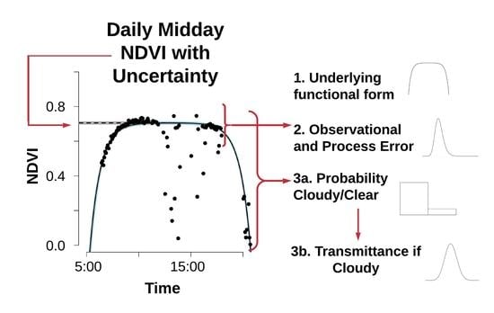
This model is fit using a Bayesian framework. In summary, the model (1) assumes that without noise, the “true” NDVI values fall along a diurnal pattern of increasing in the morning and decreasing in the afternoon (Figure 2); and (2) includes an error model that accounts for the negative bias in the noise due to atmospheric attenuation (e.g., from clouds and aerosols) by calculating the probability that each observation is clear or cloudy and the amount that the atmosphere transmits if it is “cloudy”. This methodology is provided in an R package at https://github.com/k-wheeler/NEFI_pheno/tree/master/GOESDiurnalNDVI with the goal that it can be used with limited knowledge of Bayesian statistics. A more complete description of the model is given in the following three subsections.
2.3.1. Fitting the Diurnal Curve
The general framework of this model is to fit a double exponential function, with a changepoint between the increasing and decreasing sections, to diurnal NDVI data (Figure 2). The exponential function was chosen as a process model due to the general characteristic of the data [24] (Supplementary Figure S1), because exponential fits performed better than a logistic model, and also based off of looking at thousands of diurnal time-series at deciduous broadleaf sites (e.g., Figure 2). Based on the data, the left and right sides of the diurnal cycle, μLi and μRi respectively, are calculated using the equations below:
The expected value (fi) is then calculated by:
ti denotes the time (in hours) of the ith observation. The parameter k indicates the time (in hours) where the model changes from fitting an exponential growth model to fitting an exponential decay model. This time denotes when the modeled NDVI value is at a maximum for the day. This modeled maximum midday NDVI value is represented by the parameter c (note this is the maximum of the model, which due to noise may not be the maximum observation). Based on observed patterns the diurnal cycle is assumed to be symmetric, which allows for the fitting of a curve even if NDVI values are missing in the early morning or late afternoon. Thus, the shape parameter, a, is the same for both the exponential growth and exponential decay sides. This assumption of symmetry allows for the model to converge for more days and appears to be valid for most of the days for the selected sites. However, the symmetry assumption is likely less for pixels that have highly variable terrain and in such cases separate a parameters should be fit. The parameter a controls the rate at which NDVI values increase in the early morning and decrease in the evening. The parameters a, k, and c are fit for the entire day for each GOES pixel. Graphical representations of the parameters are provided in Figure 2.
Since we fit this model in a Bayesian context all model parameters required prior distributions, which were relatively uninformed and estimated from simulated potential curves. The parameter a was assumed to have a zero truncated normal prior distribution with a mean of 0.0009 and precision (1/σ2) of 1.11 × 10⁷ (σ ~0.003) based on possible values for the time and NDVI observations. The prior on c, beta (2,1.5), was chosen because NDVI values will theoretically be between 0 and 1 for snowless vegetation, which is a characteristic of beta distributions. The parameter k was assumed to have a normal prior with a mean of 12 (noon) and a standard deviation of 1. The mean and precision were selected to allow for two standard deviations on either side to include the middle four hours of the day that are often used in window averaging.
2.3.2. Accounting for Error Due to Atmospheric Scattering
GOES NDVI data are still affected by atmospheric scattering even after the cloud mask is applied. To account for this, for each observation we model the probability that it was affected by atmospheric scattering. For each observation, the variable isCloudy follows a Bernoulli distribution describing the probability (p) of whether a cloud (or other atmospheric interference) is present or not. We set the prior on p to be uninformative and uniformly distributed between 0 and 1. Next, conditional on isCloudy, we assume that the true NDVI observation is attenuated by an atmospheric transmissivity (T) that is distributed with a beta distribution, T ~ beta (α, β), which is bounded by 0 and 1, but not uniform throughout its range. The α and β terms in the transmissivity beta distribution are given uninformative priors of both being uniformly distributed between 1 and 100. Each observation during the day receives specific isCloudy and transmissivity values.
Combining these parts, the expected mean NDVI, μi, of an observation is calculated as a weighted average between cloudy and non-cloudy states:
The observed NDVI is then modeled with Gaussian observation error, NDVIi ~ normal (μt, σ2), where the variance, σ2, is assigned an uninformative inverse-gamma (0.001, 0.00001) prior.
2.3.3. Fitting Overall Model
The overall model (i.e., the model including the components described in Section 2.3.1 and Section 2.3.2) was fit using standard Bayesian Markov Chain Monte Carlo (MCMC) approaches using JAGS called from R [20] using the rjags [25] and runjags [26] packages for all days with >10 observations. The analysis was run independently for each site and day using five chains. All models converged, as assessed using the Gelman–Brooks–Rubin statistic (GBR < 1.05), and all effective samples sizes >5000 after burn-in were removed. Model credible intervals (95%) were calculated using 10,000 random samples from the joint posterior distribution. The curve shape parameters (a, c, and k), and the statistical parameters p, α, and β each have one posterior distribution per pixel per day (Figure 2). In contrast, the posterior distributions for T and isCloudy differ for each observation. Thus, each day’s α and β distributions denote one beta distribution, which represents the distribution of the T values of the different ti throughout that day. Likewise, the distribution describing the probability of clouds is the same for each observation of the day, but the 0/1 state of whether a cloud is assumed to be obstructing a specific observation is different between observations. In addition to validating against GOES data, this method was also validated against simulated pseudo-data, which is shown in the supplementary materials Figure S2.
To understand the applicability of the presented diurnal fit method, we investigated which proportion of days fell into different categories based off of the overall noisiness of the data and the uncertainty of the midday maximum estimate. The noisiness of the data was assessed using the width of the 0.025 to 0.975 quantiles range of the data within the four-hour midday window (widths <0.1 NDVI were considered low noise). Days with <5 points within the four-hour midday window were designated as having no midday window. Days that had <0.1 wide 95% CI in the diurnal fit estimated midday maximum values were designated as having low uncertainty. In summary, the six categories were low noise and tight fit, high noise and tight fit, no window and tight fit, low noise and wide fit, high noise and wide fit, and no window and wide fit.
2.4. Comparison to Other Potential Methods
The diurnal fit model was used to estimate NDVI values throughout the year (1 July 2017 through 30 June 2018) for the fifteen deciduous broadleaf sites provided in Table 1. To compare the diurnal fit method to other simpler potential methods, midday values were also estimated based on other methods: (a) taking the noon measurement (starting at 11:57), (b) using the maximum NDVI measurement for each day, and (c) taking an average over the four midday hours (10:00−14:00) for days with at least five observations. 95% confidence intervals (CI) were also computed for the midday average method. Looking at only the noon observations was chosen because NDVI was expected to peak midday and it provided the simplest methodology. The maximum NDVI measurement was chosen to mimic the MVC technique and the midday hour window average was based on [16].
3. Results
3.1. Example Fits
In total for all sites, 3162 diurnal fits converged (>99.95% of site days with >10 observations; ~60% of all days; Figure 3). The diurnal fit method produced estimates of the midday maximum NDVI value with <0.1 uncertainty for 72% of the fit days (Figure 4). Of the days with wide fits, instances of where mid-day values had low noise or high noise were relatively rare (2% and 5% of the total, respectively). Days with less than five observations within the midday window caused most of the wide fits (19% of the total), but 13% of the days were missing the midday window, but still had tight fits. Based on comparisons to nearby days, the CI’s on the wide fits predominantly included reasonable estimates of the midday maximum values (Figure 4A,E,F), but there were occasionally days that were not within the expected seasonal magnitude (Figure 3). Overall, the diurnal fit method captured the seasonal cycle of NDVI changes (Figure 3). Additional examples from each category are provided in Figures S3–S8. The percentages of each category did not appear to systematically differ between sites and the exact numbers for each category for each site are given in Table S1.
3.2. Comparison to Other Methods
Figure 5 illustrates how midday NDVI estimates varied between the different potential methods for one example day. Figure 6 illustrates how midday NDVI estimates produced by the method proposed here compares to the other potential methods throughout a year. The diurnal fit method was able to fit to 1134 more days (76 additional days on average per site) than the window average method within the studied year. The diurnal fit method was less noisy than the other methods (Figure 6B,C). The maximum value method often produced values that were higher than those estimated from the other methods (Figure 5 and Figure 6C) and the window average method often produced values that were lower than the other methods (Figure 5 and Figure 6C). Overall the above methodology provides less biased estimates for a daily NDVI value along with an explicit estimate of uncertainty.
4. Discussion
Many of the uses of NDVI, such as sensing phenological transitions and detecting disturbances, often change over shorter time scales than sun-synchronous NDVI products are capable of measuring. With the ability to measure NDVI at five-minute intervals throughout the continental United States and ten-minute intervals throughout most of the western hemisphere, the newest versions of the GOES series (GOES-16 and GOES-17) have the high potential to provide more detailed measurements. Since the studied year was the first year of GOES-16 measurements, and included a gap in data due to the satellite being offline as it was moved to its final orbiting position, subsequent years will likely have more days that the diurnal fit method can be applied to. The high frequency of this data is particularly useful for applications requiring near real-time data, such as vegetation phenological forecasting. Even when daily NDVI estimates are not required for application at coarser timescales (e.g., seasonal), the high-frequency measurements provide the capacity to better account for clouds and some amounts of atmospheric scattering.
While fitting this model daily can be more computationally expensive than the simpler methods, we demonstrated that many other methods can be systematically biased due to atmospheric scattering and observational error. Overall, our approach was less sensitive to the accuracy of cloud and atmospheric interference masks than other previously used methods. The diurnal fit method provides less noisy daily NDVI estimates than those produced by methods that rely on only one measurement (i.e., the noon or maximum values). The maximum value method tends to produce an estimate that is too high (Figure 5 and Figure 6C) because observational error can be present above the more consistent midday estimate—given the high data volumes present in GOES, the maximum value method is essentially selecting for outliers (Figure 4B). There is also a potential error in NDVI calculations from other techniques that rely on MVC to exclude values that were lowered due to atmospheric scattering. While the maximum value method usually produces higher-biased NDVI estimates, noisy days with a low number of observations can also produce abnormally low NDVI estimates (evaluated by comparison to other midday NDVI values of nearby days; Figure 6C). The diurnal fit method instead acknowledges the high uncertainty in the estimates of those days.
Compared to the noon observation and the maximum observation methods, the midday four-hour window average has the benefit of providing a measure of uncertainty. However, because of atmospheric attenuation (e.g., clouds and scattering), more noise is present below the expected NDVI values than above them. By averaging over this window without taking into consideration this unequal distribution of error, this estimate is usually biased too low (Figure 5 and Figure 6C) and the uncertainties are underestimated. Additionally, because the diurnal fit method does not have to predesignate a window timespan, it allows for the estimation of NDVI for more days than the window average method does (76 days/year in our test example) as long as enough measurements are available before and/or after the plateau. The noon observation and window averaging methods are much more sensitive to the accuracy of the cloud mask.
We did not see large differences in algorithm performance across the different studied deciduous broadleaf sites (Table S1) suggesting that the methodology here is applicable to other forests. We only focused on deciduous broadleaf sites, which all had similar characteristic shape to the diurnal curve. Sites with sparse vegetation (e.g., shrubland systems) appeared to not as consistently have the same diurnal shape (Figure S9). This could potentially be due to the low leaf area index (LAI) in shrublands contributing to a higher influence from the background soil, which has been found to decrease the midday NDVI values [27] and is shown in supplementary Figure S9. Campbell et al. [27] found, however, that this decrease in midday NDVI values did not occur for areas with higher LAI values. NDVI values at shrubland sites appear to be less noisy due to having characteristically less clouds and precipitation and a more comprehensive statistical framework, like the one presented here, might not be as necessary, though further work needs to be done on this. While there were no noticeable differences between the types of categories of fit between different sites, there were differences in the number of days that had observations between the sites. The sites with the lowest numbers of days with observations (i.e., Hubbard Brook, Willow Creek, and Bartlett) all had decreased observations in the winter, which is likely due to snow. Snow causing noisiness in the data is common in remotely sensed NDVI data (e.g., [28]) and applying the GOES data quality flags filtered out some of these winter observations.
An alternative method for dealing with differing sun angle geometry is the bidirectional reflectance distribution function (BRDF) scheme, which interpolates nadir-equivalent band reflectance values for the pixels that have large sun angles. This calculation can be quite complicated, however, and sensor specific. Additionally, BRDF is highly dependent on an accurate cloud mask and methodology for filtering out other atmospheric scattering and noise [12]. By not using a BRDF correction scheme, our method maintains the diurnal shape that allows for a better quantification of noise throughout the day. Even though there is not yet a BRDF product for GOES that would allow us to make a direct comparison, there are reasons to believe the diurnal fit methodology should be less sensitive to the cloud mask, and handle some atmospheric scattering better than the BRDF method, since it not only accounts for diurnal variation but also for noise. When BRDF was used for NDVI calculations from the SEVIRI sensor [17], the atmospheric correction was complicated and relied on knowledge of a variety of atmospheric traits, including water vapor, ozone content, and aerosol optical depth, all of which relied on a daily MODIS atmospheric product. The methodology presented here does not apply one atmospheric scattering value per day, but instead applies a probabilistic approach to model how individual observations are potentially affected by atmospheric interferences (e.g., clouds and aerosols), thus allowing it to capture sub daily variability in atmospheric conditions (Figure 2, Figure 3 and Figure 5). BRDF, however, is still useful for correcting for solar angle differences between days of the year and different locations.
Since the satellites were still new at the time of this study, techniques were not finalized to fully correct for atmospheric scattering and only uncorrected reflectance factors were available for this analysis. The goal of this manuscript was to present a statistical model to evaluate the best estimate of NDVI for the given diurnal data. This paper presented a statistical framework that should still hold even if the magnitudes of NDVI were slightly shifted due to inherent baseline scattering/radiation within the atmosphere. For example if daily atmospheric corrections applied (e.g., [17]), sub-daily biased noise will still remain, which the methodology presented here will account for. Currently, uses of NDVI that rely on an accurate estimate of surface NDVI need to wait for further work into correcting for baseline atmospheric scattering. The diurnal fit model presented here will still stand as a less-biased statistical estimate of the midday maximum NDVI value based off of the available reflectance data. Applications, such as the monitoring of phenological change, that do not rely on previous calibrations to NDVI will still benefit from this work and do not require exact NDVI measurements.
Finally, the Bayesian methodology used here is more computationally expensive than current alternatives and at the moment is most realistic to implement at smaller scales. Additional work needs to go into investigating how to scale up this algorithm, for example by potentially leveraging the spatial and temporal autocorrelation in model parameters. It might also be possible to increase computational efficiency by leveraging more efficient sequential Bayesian methods or emulator approaches [29]. Additionally, future work could look into combining BRDF and the methodology presented here. That said, until a BRDF scheme is created for this specific sensor, the methodology presented here is both more accurate (less biased) and more precise (lower noise) than other potential methods, and provides explicit error estimates on all parameters.
5. Conclusions
Here, we presented a statistical framework to determine a daily midday estimate of NDVI over deciduous broadleaf forests that is less susceptible to biased noise and less sensitive to the accuracy of cloud masks than many simpler methods (i.e., maximum value, noon observation, and average over midday observations). The performance of the presented diurnal fit method performed consistently across sites, indicating that the method is applicable at other deciduous broadleaf sites. The advanced baseline imager on GOES-16 and GOES-17 provides the ability to monitor NDVI at high temporal resolutions, which will improve the ability to monitor a variety of ecosystem processes.
Supplementary Materials
The following are available online at https://www.mdpi.com/2072-4292/11/21/2507/s1, description of methods for simulation of pseudo-data, Figures S1–S9, Table S1.
Author Contributions
Conceptualization, K.I.W. and M.C.D.; methodology, K.I.W. and M.C.D.; software, K.I.W.; validation, K.I.W.; formal analysis, K.I.W.; writing—original draft preparation, K.I.W.; writing—review and editing, K.I.W. and M.C.D.; visualization, K.I.W.; supervision, M.C.D.; funding acquisition, K.I.W. and M.C.D.
Funding
This work was made possible by US National Science Foundation grant 1638577. KIW was also supported under the National Science Foundation Graduate Research Fellowship grant number 1247312.
Acknowledgments
Special thanks to the Near-term Ecological Forecasting Initiative team and Dietze lab members for feedback on the manuscript.
Conflicts of Interest
The authors declare no conflict of interest.
References
- Zhang, X.; Friedl, M.A.; Schaaf, C.B.; Strahler, A.H.; Hodges, J.C.F.; Gao, F.; Reed, B.C.; Huete, A. Monitoring vegetation phenology using MODIS. Remote Sens. Environ. 2003, 84, 471–475. [Google Scholar] [CrossRef]
- Loveland, T.R.; Reed, B.C.; Brown, J.F.; Ohlen, D.O.; Zhu, Z.; Yang, L.; Merchant, J.W. Development of a global land cover characteristics database and IGBP DISCover from 1 km AVHRR data. Int. J. Remote Sens. 2000, 21, 1303–1330. [Google Scholar] [CrossRef]
- Lunetta, R.S.; Knight, J.F.; Ediriwickrema, J.; Lyon, J.G.; Worthy, L.D. Land-cover change detection using multi-temporal MODIS NDVI data. Remote Sens. Environ. 2006, 105, 142–154. [Google Scholar] [CrossRef]
- Jacquin, A.; Sheeren, D.; Lacombe, J.-P. Vegetation cover degradation assessment in Madagascar savanna based on trend analysis of MODIS NDVI time series. Int. J. Appl. Earth Obs. Geoinf. 2010, 12, S3–S10. [Google Scholar] [CrossRef] [Green Version]
- Gamon, J.A.; Field, C.B.; Goulden, M.L.; Griffin, K.L.; Hartley, A.E.; Joel, G.; Peñuelas, J.; Valentini, R. Relationships Between NDVI, Canopy Structure, and Photosynthesis in Three Californian Vegetation Types. Ecol. Appl. 1995, 5, 28–41. [Google Scholar] [CrossRef] [Green Version]
- Wang, Q.; Adiku, S.; Tenhunen, J.; Granier, A. On the relationship of NDVI with leaf area index in a deciduous forest site. Remote Sens. Environ. 2005, 94, 244–255. [Google Scholar] [CrossRef]
- Nolè, A.; Rita, A.; Ferrara, A.M.S.; Borghetti, M. Effects of a large-scale late spring frost on a beech (Fagus sylvatica L.) dominated Mediterranean mountain forest derived from the spatio-temporal variations of NDVI. Ann. For. Sci. 2018, 75, 83. [Google Scholar] [CrossRef] [Green Version]
- Parker, G.; Martínez-Yrízar, A.; Álvarez-Yépiz, J.C.; Maass, M.; Araiza, S. Effects of hurricane disturbance on a tropical dry forest canopy in western Mexico. For. Ecol. Manag. 2018, 426, 39–52. [Google Scholar] [CrossRef]
- Pettorelli, N.; Vik, J.O.; Mysterud, A.; Gaillard, J.-M.; Tucker, C.J.; Stenseth, N.C. Using the satellite-derived NDVI to assess ecological responses to environmental change. Trends Ecol. Evol. 2005, 20, 503–510. [Google Scholar] [CrossRef]
- Bino, G.; Levin, N.; Darawshi, S.; Van Der Hal, N.; Reich-Solomon, A.; Kark, S. Accurate prediction of bird species richness patterns in an urban environment using Landsat-derived NDVI and spectral unmixing. Int. J. Remote Sens. 2008, 29, 3675–3700. [Google Scholar] [CrossRef]
- Fernandez, A. Automatic mapping of surfaces affected by forest fires in Spain using AVHRR NDVI composite image data. Remote Sens. Environ. 1997, 60, 153–162. [Google Scholar] [CrossRef]
- Huete, A.; Didan, K.; Miura, T.; Rodriguez, E.P.; Gao, X.; Ferreira, L.G. Overview of the radiometric and biophysical performance of the MODIS vegetation indices. Remote Sens. Environ. 2002, 83, 195–213. [Google Scholar] [CrossRef]
- Borgogno-Mondino, E.; Lessio, A.; Gomarasca, M.A. A fast operative method for NDVI uncertainty estimation and its role in vegetation analysis. Eur. J. Remote Sens. 2016, 49, 137–156. [Google Scholar] [CrossRef]
- Schmit, T.J.; Griffith, P.; Gunshor, M.M.; Daniels, J.M.; Goodman, S.J.; Lebair, W.J. A Closer Look at the ABI on the GOES-R Series. Bull. Am. Meteorol. Soc. 2016, 98, 681–698. [Google Scholar] [CrossRef]
- GOES-R Calibration Working Group. NOAA GOES-R Series Advanced Baseline Imager (ABI) Level 1b Radiances. [Channels 2 and 3]; GOES-R Series Program; NOAA National Centers for Environmental Information: Asheville, NC, USA, 2017.
- Fensholt, R.; Sandholt, I.; Stisen, S.; Tucker, C. Analysing NDVI for the African continent using the geostationary meteosat second generation SEVIRI sensor. Remote Sens. Environ. 2006, 101, 212–229. [Google Scholar] [CrossRef]
- Proud, S.R.; Zhang, Q.; Schaaf, C.; Fensholt, R.; Rasmussen, M.O.; Shisanya, C.; Mutero, W.; Mbow, C.; Anyamba, A.; Pak, E.; et al. The Normalization of Surface Anisotropy Effects Present in SEVIRI Reflectances by Using the MODIS BRDF Method. IEEE Trans. Geosci. Remote Sens. 2014, 52, 6026–6039. [Google Scholar] [CrossRef]
- Zeng, Y.; Li, J.; Liu, Q.; Huete, A.R.; Xu, B.; Yin, G.; Zhao, J.; Yang, L.; Fan, W.; Wu, S.; et al. An Iterative BRDF/NDVI Inversion Algorithm Based onA PosterioriVariance Estimation of Observation Errors. IEEE Trans. Geosci. Remote Sens. 2016, 54, 6481–6496. [Google Scholar] [CrossRef]
- Kahle, D.; Wickham, H. ggmap: Spatial Visualization with ggplot2. R J. 2013, 5, 144–161. [Google Scholar] [CrossRef] [Green Version]
- R Core Team. R: A Language and Environment for Statistical Computing; R Foundation for Statistical Computing: Vienna, Austria, 2017. [Google Scholar]
- Hijmans, R.J.; Cameron, S.E.; Parra, J.L.; Jones, P.G.; Jarvis, A. Very high resolution interpolated climate surfaces for global land areas. Int. J. Climatol. 2005, 25, 1965–1978. [Google Scholar] [CrossRef]
- PhenoCam Provisional Data for Site Harvard; Hubbardbrooksfws; Umichbiological; Coweeta; Bartlettir; Missouriozarks; Morganmonroe; Russellsage; Willowcreek; Bullshoals; Dukehw; Greenridge1; Shenandoah; Marcel; Shiningrock. Available online: http:phenocam.sr.unh.edu (accessed on 30 November 2017).
- Thieurmel, B.; Elmarhraoui, A. suncalc: Compute Sun Position, Sunlight Phases, Moon Position and Lunar Phase. 2019. Available online: https://rdrr.io/cran/suncalc/ (accessed on 1 August 2019).
- Schaepman-Strub, G.; Schaepman, M.E.; Painter, T.H.; Dangel, S.; Martonchik, J.V. Reflectance quantities in optical remote sensing—definitions and case studies. Remote Sens. Environ. 2006, 103, 27–42. [Google Scholar] [CrossRef]
- Plummer, M. rjags: Bayesian Graphical Models Using MCMC. 2018. Available online: https://rdrr.io/cran/rjags/ (accessed on 1 July 2018).
- Denwood, M.J. runjags: An R Package Providing Interface Utilities, Model Templates, Parallel Computing Methods and Additional Distributions for MCMC Models in JAGS. J. Stat. Softw. 2016, 71, 1–25. [Google Scholar] [CrossRef]
- Campbell, P.K.E.; Huemmrich, K.F.; Middleton, E.M.; Ward, L.A.; Julitta, T.; Daughtry, C.S.T.; Burkart, A.; Russ, A.L.; Kustas, W.P. Diurnal and Seasonal Variations in Chlorophyll Fluorescence Associated with Photosynthesis at Leaf and Canopy Scales. Remote Sens. 2019, 11, 488. [Google Scholar] [CrossRef]
- Zhang, Q.; Xiao, X.; Braswell, B.; Linder, E.; Ollinger, S.; Smith, M.-L.; Jenkins, J.P.; Baret, F.; Richardson, A.D.; Moore, B.; et al. Characterization of seasonal variation of forest canopy in a temperate deciduous broadleaf forest, using daily MODIS data. Remote Sens. Environ. 2006, 105, 189–203. [Google Scholar] [CrossRef]
- Fer, I.; Kelly, R.; Moorcroft, P.R.; Richardson, A.D.; Cowdery, E.M.; Dietze, M.C. Linking big models to big data: Efficient ecosystem model calibration through Bayesian model emulation. Biogeosci. Discuss. 2018, 15, 1–30. [Google Scholar] [CrossRef]

Figure 2.
Depiction of the model using an example from one day (2017-08-19) at Russell Sage. The central plot indicates the normalized difference vegetation index (NDVI) observations in black points. The solid curve line represents the median model fit. The solid horizontal and vertical lines indicate the mean values for the parameters c and k, respectively. Except for the distributions surrounded by a box, the parameter distributions indicate the posterior distributions over all of the samples. The boxes around the transmissivity (T) and isCloudy (clear vs. cloudy) indicate that these are the distributions of the values for the observations of one sample of the one day using the posterior means of the parameters p, α, and β.

Figure 3.
Time-series for the fifteen deciduous sites (labeled on the y-axis besides each time-series) for the midday maximum NDVI values fitted from the diurnal fit method. The tick marks on the y-axis indicate 0.0 NDVI for the site labeled above the tick and 1.0 NDVI for the site labeled below the tick. The shading of the points is scaled to be proportional to the width of the 95% credible interval (CI) of each NDVI estimate (i.e., estimates with smaller uncertainties are darker). The CI’s are provided as vertical lines with the same shading. Sites are ordered (top-to-bottom, left panel to right panel) by the total number of days with >10 observations (Bull Shoals had the most and Hubbard Brook had the least). The majority of the diurnal fit estimates with a tight CI fall along the expected seasonal pattern for NDVI and estimates that do not usually have a high uncertainty.

Figure 4.
Example fits for six days of the year at different sites. The blue shading around the diurnal curve indicates the 95% credible interval for the black observation points. The black line indicates the mean fit for that day and the percentage given indicates the frequency of the category within the studied days. (A) The diurnal fit for 2018-01-30 at Hubbard Brook. (B) The diurnal fit for 2017-07-08 at Marcell. (C) The diurnal fit for 2018-05-24 at Morgan Monroe. (D) The diurnal fit for 2017-10-17 (blue shading and black points and line) and 2017-10-13 (orange shading) for comparison at Harvard Forest. (E) The diurnal fit for 2018-05-10 (blue shading and black points and line) and 2018-05-11 (orange shading) at Shining Rock. (F) The diurnal fit for 2018-05-10 (blue shading and black points and line) and 2018-05-11 at Shenandoah. The diurnal fit method produces estimates of the midday maximum NDVI value even when there is noise or <5 observations within the midday window.

Figure 5.
Plot showing that methods can produce vastly different NDVI values based on how susceptible they are to noise. The expected maximum/midday NDVI values are shown in solid lines. The blue background shading indicates the 95% CI on the window average. The 95% CI on the diurnal fit estimate (red shading) is barely visible. Two potential noon measurements (11:57 and 12:02) are given to show the sensitivity to noise this method has. The diurnal fit method is less sensitive to noise and biases than the other potential methods of maximum, noon value, and midday window average.

Figure 6.
Example time series showing how the daily midday NDVI determined using the proposed model compares to some other potential options throughout the year (2017-07-01 through 2018-06-30) at Russell Sage. The black points in all panels indicate the diurnal fitted estimate. (A) Comparison of the diurnal fitted estimates to the noon observations (11:57am). (B) Comparison of the diurnal fitted estimates to the daily maximum observations. (C) Comparison of the diurnal fitted estimates to the four-hour midday average. Vertical lines in all panels indicate 95% CI’s for those methods that provide a measure of uncertainty. The other potential methods have systematic biases associated with them throughout the year: noon measurement is noisy without an estimate of uncertainty, maximum measurement is often biased too high, and midday average is often biased too low.


Table 1.
Characteristics of the chosen deciduous broadleaf sites. Climate data are from WorldClim [21] and elevation data are from the PhenoCam Network [22]. Sites are ordered based off of the number of days that had >10 observations within the year.
| Site Name | Latitude | Longitude | Mean Annual Temperature (°C) | Mean Annual Precipitation (mm) | Elevation (m) |
|---|---|---|---|---|---|
| Bull Shoals | 36.563 | −93.067 | 13.9 | 1084 | 260 |
| Russell Sage | 32.457 | −91.974 | 18.1 | 1341 | 20 |
| Duke | 35.974 | −79.100 | 14.6 | 1166 | 400 |
| Marcell | 47.514 | −93.469 | 2.9 | 687 | 422 |
| Missouri Ozarks | 38.744 | −92.200 | 12.4 | 974 | 219 |
| UMBS | 45.560 | −84.714 | 5.9 | 797 | 230 |
| Coweeta | 35.060 | −83.428 | 12.5 | 1722 | 680 |
| Shenandoah | 38.617 | −78.350 | 8.4 | 1222 | 1037 |
| Shining Rock | 35.390 | −82.775 | 9.3 | 1835 | 1500 |
| Harvard Forest | 42.538 | −72.172 | 6.8 | 1139 | 340 |
| Green Ridge | 39.691 | −78.407 | 10.5 | 935 | 285 |
| Morgan Monroe | 39.323 | −86.413 | 11.2 | 1087 | 275 |
| Bartlett | 44.065 | −71.288 | 5.5 | 1224 | 268 |
| Willow Creek | 45.806 | −90.079 | 3.9 | 820 | 521 |
| Hubbard Brook | 43.927 | −71.741 | 4.6 | 1190 | 253 |
© 2019 by the authors. Licensee MDPI, Basel, Switzerland. This article is an open access article distributed under the terms and conditions of the Creative Commons Attribution (CC BY) license (http://creativecommons.org/licenses/by/4.0/).
Share and Cite
MDPI and ACS Style
Wheeler, K.I.; Dietze, M.C. A Statistical Model for Estimating Midday NDVI from the Geostationary Operational Environmental Satellite (GOES) 16 and 17. Remote Sens. 2019, 11, 2507. https://doi.org/10.3390/rs11212507
AMA Style
Wheeler KI, Dietze MC. A Statistical Model for Estimating Midday NDVI from the Geostationary Operational Environmental Satellite (GOES) 16 and 17. Remote Sensing. 2019; 11(21):2507. https://doi.org/10.3390/rs11212507
Chicago/Turabian StyleWheeler, Kathryn I., and Michael C. Dietze. 2019. "A Statistical Model for Estimating Midday NDVI from the Geostationary Operational Environmental Satellite (GOES) 16 and 17" Remote Sensing 11, no. 21: 2507. https://doi.org/10.3390/rs11212507
Note that from the first issue of 2016, this journal uses article numbers instead of page numbers. See further details here.