Methane Emission Estimates by the Global High-Resolution Inverse Model Using National Inventories

Abstract

We present a global 0.1° × 0.1° high-resolution inverse model, NIES-TM-FLEXPART-VAR (NTFVAR), and a methane emission evaluation using the Greenhouse Gas Observing Satellite (GOSAT) satellite and ground-based observations from 2010–2012. Prior fluxes contained two variants of anthropogenic emissions, Emissions Database for Global Atmospheric Research (EDGAR) v4.3.2 and adjusted EDGAR v4.3.2 which were scaled to match the country totals by national reports to the United Nations Framework Convention on Climate Change (UNFCCC), augmented by biomass burning emissions from Global Fire Assimilation System (GFASv1.2) and wetlands Vegetation Integrative Simulator for Trace Gases (VISIT). The ratio of the UNFCCC-adjusted global anthropogenic emissions to EDGAR is 98%. This varies by region: 200% in Russia, 84% in China, and 62% in India. By changing prior emissions from EDGAR to UNFCCC-adjusted values, the optimized total emissions increased from 36.2 to 46 Tg CH₄ yr⁻¹ for Russia, 12.8 to 14.3 Tg CH₄ yr⁻¹ for temperate South America, and 43.2 to 44.9 Tg CH₄ yr⁻¹ for contiguous USA, and the values decrease from 54 to 51.3 Tg CH₄ yr⁻¹ for China, 26.2 to 25.5 Tg CH₄ yr⁻¹ for Europe, and by 12.4 Tg CH₄ yr⁻¹ for India. The use of the national report to scale EDGAR emissions allows more detailed statistical data and country-specific emission factors to be gathered in place compared to those available for EDGAR inventory. This serves policy needs by evaluating the national or regional emission totals reported to the UNFCCC.

1. Introduction

The average global atmospheric methane concentration had reached 1867 ppb by the end of the year 2018 and is rising faster than at any time in the past two decades, while the carbon dioxide (CO₂) increase is slowing down [1,2,3]. Methane (CH₄) plays a growing role in anthropogenic climate change with its share of more than 20% of the total greenhouse gas (GHG) concentration [4,5,6]. Reducing methane emissions would make a significant contribution to climate change mitigation on a shorter time scale, due to its relatively short lifetime compared with that of CO₂ [7,8]. The determination of national emission reduction targets and policies is directly affected by the amount of methane emissions produced by individual countries [9]. However, studies on emission estimates suggest that there are still large uncertainties in methane budgets, and more effort should be made to better quantify the methane emissions [10,11,12,13,14,15]. Still, it is challenging to verify the accuracy of methane emissions on a country scale. The national reports submitted to the United Nations Framework Convention on Climate Change (UNFCCC) by different countries might use different methods to estimate emissions, which could be different from global inventory datasets produced by the scientific community, such as the Global Carbon Project (GCP) [16], and the Emissions Database for Global Atmospheric Research (EDGAR) [17,18,19]. Complementary to these bottom-up emission estimations, top-down estimations by inverse models combined with atmospheric measurements have been widely used and have proven worthy for emission inventory evaluation (e.g., [20,21,22,23,24,25,26]). Houweling et al. [27] reviewed the development of global inverse modeling of methane, and Jacob et al. [28] also supported their research by presenting the advantages of increased observational data from surface stations, satellites and aircraft, and state-of-the-art computational facilities. The inverse model has become more important for allowing better quantification of methane emissions.

Studies have shown an extension of regional Lagrangian inverse modelling to global scale inverse modeling based on a combination of the 3D global Eulerian models and the Lagrangian models (e.g., [29,30]). They have demonstrated an enhanced capability of the transport resolving high resolution surface emission patterns using inverse modeling schemes relying on regional and global basis flux patterns. The disadvantage of using regional basis functions in inverse modeling has been addressed by developing grid-based inversion schemes that use variational assimilation algorithms (e.g., [22,31,32,33]). To implement a grid-based inversion scheme suitable for optimizing surface fluxes at the high resolution of the Lagrangian model, an adjoint of a coupled Eulerian–Lagrangian model is needed. Maksyutov et al. [34] developed the global 0.1° × 0.1° high spatial resolution inverse model NIES-TM-FLEXPART-VAR (NTFVAR), which provides an extension of the high resolution regional inverse modeling approaches [22,31,32,33] on a global scale. The NTFVAR model is a grid-based inversion scheme that is suitable for optimizing surface fluxes at high resolution, providing the capability to use high-resolution regional transport with global mass conservation and consistency of the estimated regional fluxes with global concentration trends. This paper presents the estimation of global and regional methane emissions using the NTFVAR inverse modeling system with two sets of emission inventories that differ in anthropogenic emissions—one with anthropogenic emissions from EDGAR v4.3.2 and the other with anthropogenic emissions from EDGAR v4.3.2 scaled to UNFCCC national reports [35].

2. Materials and Methods

2.1. Inverse Modeling System—NTFVAR

2.1.1. The Transport Model

We used a global Eulerian–Lagrangian coupled model NIES-TM-FLEXPART-VAR (NTFVAR) that consists of the National Institute for Environmental Studies (NIES) model as a Eulerian three-dimensional transport model (TM), and FLEXPART (FLEXible PARTicle dispersion model) as the Lagrangian Particle Dispersion Model (LPDM). The forward transport model and model development were described by Ganshin et al. [36] and Belikov et al. [30], and the application to inverse modeling using the Kalman smoother at moderate resolution of 1° × 1° was demonstrated by Zhuravlev et al. [37], Ishizawa et al. [38], and Shirai et al. [29]. Our transport model is a further modification of the model described by Belikov et al. [30]. The coupled model combines National Institute for Environmental Studies Transport Model (NIES-TM) v08.1i with a horizontal resolution of 2.5° and 32 hybrid-isentropic vertical levels [39] and Flexpart model v.8.0 [40], and runs in backward mode with a surface flux resolution of 0.1°. The changes in the current version with respect to the study by Belikov et al. [30] include the derivation of adjoint components using the adjoint code compiler Tapenade [41] instead of the TAF (Transformation of Algorithms in Fortran) compiler [42]. Additionally, the transport matrix indexing and sorting algorithms were revised to allow efficient memory usage for handling large matrixes of Lagrangian responses to surface fluxes required for the application of the model to satellite data. A manually- derived adjoint of the NIES TM v08.1i was used, as in Belikov et al. [30], due to its computational efficiency. The second-order approximation Van Leer algorithm [43] was implemented in the adjoint and forward models, alternatively to the third order algorithm typically used in forward models [39]. The meteorological data used for the transport model were obtained from the Japanese Meteorological Agency (JMA) Climate Data Assimilation System (JCDAS) [44,45], which provided the required parameters, such as three-dimensional wind fields, temperature, and humidity at 1.25° × 1.25° spatial resolution, 40 vertical hybrid sigma-pressure levels, and a temporal resolution of 6 h.

2.1.2. The Inverse Modeling Scheme

The same inversion scheme with high resolution (0.1° × 0.1°) fluxes and variational optimization was applied to estimate CO₂ fluxes by Maksyutov et al. [34], who also demonstrated its capability to capture the observed atmospheric CO₂ time series. In this study, the high-resolution variant of the transport model and its adjoint described by Belikov et al. [30] were combined with the optimization scheme proposed by Meirink et al. [46] and Basu et al. [47]. Following the approach by Meirink et al. [46], flux corrections were estimated independently for two categories of emissions (anthropogenic and natural). Variational optimization was applied to obtain flux corrections as two sets of scaling factors to vary prior uncertainty fields on a monthly basis at a 0.1° × 0.1° resolution separately for anthropogenic and natural wetland emissions with bi-weekly time steps. Anthropogenic emission corrections were proportional to the monthly climatology emissions provided by EDGAR, and the wetland emission corrections were proportional to the monthly climatology wetland emissions provided by the Vegetation Integrative Simulator for Trace Gases (VISIT) model (details of prior fluxes given in Section 2.2), with both given as prior uncertainty fields. The grid scale flux uncertainty was defined as 30% of the EDGAR climatology for the anthropogenic flux category and 50% of the VISIT climatological emissions for the wetland emissions category. Other flux categories, such as biomass burning, geological, termites, and soil sink, were not corrected by inversion. The spatial correlation of 500 km and temporal correlation of two weeks were used to provide smoothness constraints on the resulting fields of the scaling factors. The inverse modeling problem was formulated (e.g., Tarantola [48], Meirink et al. [46]) and solved to find the optimal value of $x$—vectors of corrections to prior fluxes at the minimum of the cost function $J\left(x\right)$:

$$J\left(x\right)=\frac{1}{2}{\left(H·x-r\right)}^T·R^{-1}·\left(H·x-r\right)+\frac{1}{2}{x}^T·B^{-1}·x$$

(1)

where $r$ is the residual (difference between the observed concentration and the forward simulation made with prior fluxes without correction), $R$ is the covariance matrix of observations, and $B$ is the covariance matrix of fluxes. In our design of matrix $B$, we follow Meirink et al. [46] in representing matrix $B$ as a multiple of the non-dimensional covariance matrix $C$ and the diagonal flux uncertainty $D$ as $B=D^T·C·D$. Matrix $C$ is commonly implemented as the band matrix with non-diagonal elements declining as $~\exp \left(-x^2/l^2\right)$ with the distance $x$ between the grid cells. To achieve computational efficiency for the flux covariance operator, the implicit diffusion technique was used to implement a spatial covariance matrix, as in Weaver and Courtier’s study [48]. To construct symmetric matrix $C$, we first implemented the square root of $C$ by implicit diffusion and constructed the adjoint of it by applying an adjoint code compiler, Tapenade, to the Fortran code of modules approximating the square root of $C$. The temporal covariance matrixes were of low dimension and were designed as in Meirink et al., 2008 by deriving the square root of the Gaussian-shaped time covariance matrix with direct Singular Value Decomposition (SVD) [49]. The optimal solution was calculated as the minimum of the cost function $J$. This was done iteratively with the efficient Broyden–Fletcher–Goldfarb–Shanno (BFGS) algorithm, as implemented by Gilbert and Lemarechal [50]. We limited the number of iterations to 40, as cost function reduction slows down by the time that this number is reached.

2.2. Prior Fluxes and Observations

Prior methane fluxes used in the coupled model included anthropogenic emissions, biospheric emissions of wetlands, soil sinks, emissions from biomass burning, and other natural sources from the ocean, geological sources, and termites. EDGAR provides an annually gridded anthropogenic emission dataset that is available at a resolution of 0.1° × 0.1° [19]. The seasonal cycle was found to have effects on the top-down emission estimation [33]. In this study, monthly variation of anthropogenic emissions was prepared based on the climatology data issued by EDGAR for 2010. The ratio of monthly emissions to annual emissions was calculated for each grid. Then, for other years, the grid value for each month was calculated proportionally to the annual grid emission of the corresponding year. The VISIT model simulations for wetlands (Cao mechanism [51]) and soil sink (Curry mechanism [52]) are available at 0.5° [53]. For simulations in this study, we updated the data by remapping the wetland emissions from 0.5° to 0.1° using the Global Lakes and Wetlands Database (GLWD) wetland area map at a resolution of 30 arcseconds [54], while soil sink data were remapped to a resolution of 0.1° using the gross primary productivity (GPP) maps by the MODIS MOD17 GPP product [55]. For emissions from biomass burning, daily Global Fire Assimilation System (GFASv1.2) [56] data were used. The oceanic, geological, and termite emissions were taken from Patra et al. [57].

The total column-averaged dry-air mole fraction (XCH₄) retrieved from the Greenhouse Gas Observing Satellite (GOSAT) (NIES Level 2 retrievals, v. 02.72) from 2010–2012 was used to constrain methane emissions. The vertical sensitivity of the GOSAT observations given by the column averaging kernel [58] was examined using 2010–2012 simulations. The root-mean-square error (RMSE) of the total methane flux was 4.5 Tg CH₄ yr⁻¹, or 0.82% of the mean total flux, and the retrieval-averaging kernel of GOSAT retrievals was not applied in this study.

In addition to the GOSAT retrievals, ground-based atmospheric methane observations from global surface sites, aircrafts, and ship tracks were used in the inversions (see Appendix A). The data contained weekly and continuous samples. The continuous observations were analyzed at the hourly scale, which was further averaged to daily means using 12:00–16:00 LT (except for mountain sites, where 0:00–4:00 LT was used). Where sampling flags were available, we pre-filtered the continuous weekly and hourly observations by selecting those with well-mixed conditions. Data uncertainty, used as the diagonal of R in Equation (1), included both the observation uncertainty (e.g., measurement error and spatial representativeness) and the transport model error. For the ground-based sites, data uncertainty was defined based on the average RMSE between the observations and prior atmospheric CH₄ generated by the NTFVAR model with the prior emissions (original EDGAR plus natural sources) for each site. The minimum uncertainty was set to 6 ppb in order to allow more freedom for the inversion in the southern hemisphere. Note that we did not apply any temporal variations to the data uncertainty. The rejection threshold of the ground-based sites was set to two times the data uncertainty. The data uncertainty for the GOSAT retrieval was set to 60 ppb with a rejection threshold of 30 ppb. Large data uncertainty was applied to the GOSAT retrievals, because the amount of GOSAT data is generally much larger than that of ground-based observations and using an insufficient data uncertainty may result in over-fitting the GOSAT data, although the measurement precision is higher for ground-based observations.

2.3. Flux Estimation Uncertainties

Estimation uncertainties were simulated by randomly perturbing the observations and the prior fluxes following the method described by Chevallier et al. [59]. We perturbed five sets of observations consistently with the observation uncertainty at each site and produced five sets of perturbed monthly EDGAR and VISIT fluxes with a random scaling factor applied separately for each GCP region and each month. The perturbation amplitude for the regional scaling factor was limited by the uncertainty scale described in Section 2.2. We then performed an inversion using the perturbed pseudo-observations as measurement data and the perturbed fluxes (perturbed EDGAR and VISIT combined with the non-perturbed soil sink, biomass burning, and other natural emissions from the ocean, geological sources, and termites) as the prior fluxes and compared the inversion results to get the standard deviation of the estimated emissions.

2.4. Adjusting Prior Anthropogenic Emissions to National Reports

EDGAR is a widely used, gridded emission inventory, and the UNFCCC reports only include the total annual emissions for each country. Annex I countries submit complete inventories of GHG emission sources and sinks from the base year (1990), and other countries are encouraged to submit their GHG inventories as part of their National Communications and Biennial Update Reports (BUR). To date, 150 countries have submitted one or more national communications with a summary of the GHG inventory. We compared the total CH₄ emissions with land use, land-use change, and forestry (LULUCF) sectors in UNFCCC reports (units: Gg) with the latest EDGAR v4.3.2 emission inventory which extended the emissions to 2012. The top fifteen emitting countries based on the EDGAR estimate for 2012 and other countries, including Germany, France, the United Kingdom, and Japan, were selected to adjust the inventory according to the UNFCCC reports. The countries selected are shown in

Table 1. The selected countries with high emissions and their methane emissions estimated by the Emissions Database for Global Atmospheric Research (EDGAR) v4.3.2 in 2012 and the United Nations Framework Convention on Climate Change (UNFCCC) in 2012 or the latest report by several non-Annex I countries (year in brackets).

Country Name	China	India	United States	Brazil	Russian Federation	Indonesia	Nigeria	Pakistan	Iran	Mexico
EDGAR (Gg)	66,297	32,582	25,770	19,212	17,441	12,027	7252	7213	6528	5201
UNFCCC (Gg)	55,914	19,776 (2010)	27,099	16,808	33,894	11,257 (2000)	4207 (2000)	2890 (1994)	3606 (2000)	4558
Country Name	Australia	Thailand	Bangladesh	Canada	Argentina	Germany	France	United Kingdom	Japan
EDGAR (Gg)	4987	4893	4808	4679	4562	2768	2651	2624	1850
UNFCCC (Gg)	4550	3171 (1994)	1191 (1994)	3939	3900	2340	2420	2424	1317

, and these nineteen countries emit 66% of the total global methane emissions according to the values estimated by EDGAR v4.3.2 for the year 2012.

The new gridded emission inventory based on the UNFCCC reports was produced by scaling the annual total value to the EDGAR estimation using Equation (2):

$$E_{UNFCCC}\left(t\right)=E_{EDGARv\mathrm{4.3.2}}\left(t\right)\times \frac{1}{n}{{\displaystyle \sum }}_{k=1}^n\left(\frac{E_{UNFCCC}\left(i\right)}{E_{EDGARv\mathrm{4.3.2}}\left(i\right)}\right)$$

(2)

where $t$ is the year (2010, 2011, or 2012); $n$ is the number of reports to the UNFCCC by the top emitting countries listed in Table 1; $\mathrm{and} i$ is the recent four reporting years, from 2009 to 2012.

For the remaining countries, $E_{UNFCCC}\left(t\right)=E_{EDGARv\mathrm{4.3.2}}\left(t\right)$.

3. Results and Discussion

3.1. Comparison of EDGAR v4.3.2 and UNFCCC Reports

We compared the annual total methane emissions from national reports of the UNFCCC and EDGAR for the top emitting countries (Figure 1). The global anthropogenic methane emissions stayed stable from 1990 to 2000 and increased again at the start of the 21st century [60]. The main sources of methane, the production and transmission of coal, oil and natural gas, livestock, waste, and wastewater, along which coal mining, livestock, and natural gas production and distribution have contributed the most to the increase in the last ten years [19]. Countries with the largest absolute increases over these ten years were China, India, Brazil, and Indonesia, whereas the largest decreases occurred in the European Union, Russian Federation, Nigeria, and Ukraine [59].

We divided countries into three groups according to the ratio of the UNFCCC-reported emissions to those by EDGAR. In the first group, G1, shown in Figure 1, Russia reported 1.7 to 2-fold of the EDGAR estimates. Some part of this increase might be due to accidental methane release, which is not included in EDGAR and is not a negligible methane source in Russia [61]. The differences reported by most countries in the second group, G2, were within 20%. The United States of America (USA) reported within 10% more than EDGAR estimate. China reported 66.3 Tg in the year 2012, which is 16% lower than the EDGAR estimate. France and the United Kingdom reported lower but within 10% of the EDGAR estimates and Germany reported 17% less than the EDGAR estimate. In the third group, G3, Japan and India reported 60%~70% of the EDGAR estimate, while Bangladesh and Iran updated their last reports in 2005 and 2000, estimating less than 50% of the EDGAR estimates.

3.2. Estimation of Global Methane Emissions

The analysis in this study was based on bi-weekly emissions estimated for the years 2010–2012 using the inverse modeling system with variational optimization to two categories of fluxes: anthropogenic and natural (wetlands). Monthly emissions were calculated and analyzed for two sets of simulations: S0 simulation with EDGAR v4.3.2 and S1 simulation with EDGAR scaled to UNFCCC reports.

The global total anthropogenic emissions estimated by EDGAR were 347 Tg CH₄ yr⁻¹ (average 2010–2012) while EDGAR adjusted to UNFCCC reports gave 338 Tg CH₄ yr⁻¹ (98% of EDGAR). The global total natural emissions from wetlands and biomass burning were 204 Tg CH₄ yr⁻¹. The global total prior methane emissions were 557 Tg CH₄ yr⁻¹ for S0 and 548 Tg CH₄ yr⁻¹ for S1. The optimized global anthrophonic emissions were 350 Tg CH₄ yr⁻¹ and 344 Tg CH₄ yr⁻¹ for S0 and S1, respectively. The optimized global total methane emissions were 572 Tg CH₄ yr⁻¹ and 566 Tg CH₄ yr⁻¹ for S0 and S1, respectively. The differences between the total methane emissions reduced from the prior values after inversion. Those results are slightly higher than the previous estimation of ${548}_{-22}^{+21}$ Tg CH₄ yr⁻¹ reported by Kirschke et al. [14] and the Intergovernmental Panel on Climate Change (IPCC) [62].

Figure 2 shows the average monthly global total and anthropogenic prior and estimated emissions. The inverse model produced lower emissions in winter compared with prior emissions and enhanced emissions in summer. Case S0 showed a more pronounced summer peak compared to case S1. The summer maximum appeared in July–August with its larger share of emissions from natural sources (e.g., wetlands, biomass burning, and lakes) and the agriculture sector [63] when minimum CH₄ concentrations were recorded in most places of the northern hemisphere due to the larger CH₄ sink as a result of the strong chemical reaction with OH in the warm season [64]. Significant differences were found between the prior and posterior fluxes in winter and summer. Since seasonal cycle separation depends on latitude and the average time period, Figure 2a shows the average for three entire years and the whole region for both prior and posterior fluxes. Figure 2b shows the monthly variation of wetland emissions and anthropogenic emissions in selected regions including boreal America, the contiguous USA, Europe, Russia, and China in the northern hemisphere, where the wetland emissions were low in winter and the difference between prior and posterior anthropogenic emissions was more independent from wetland emission uncertainties.

3.3. Estimation of Regional Methane Emissions

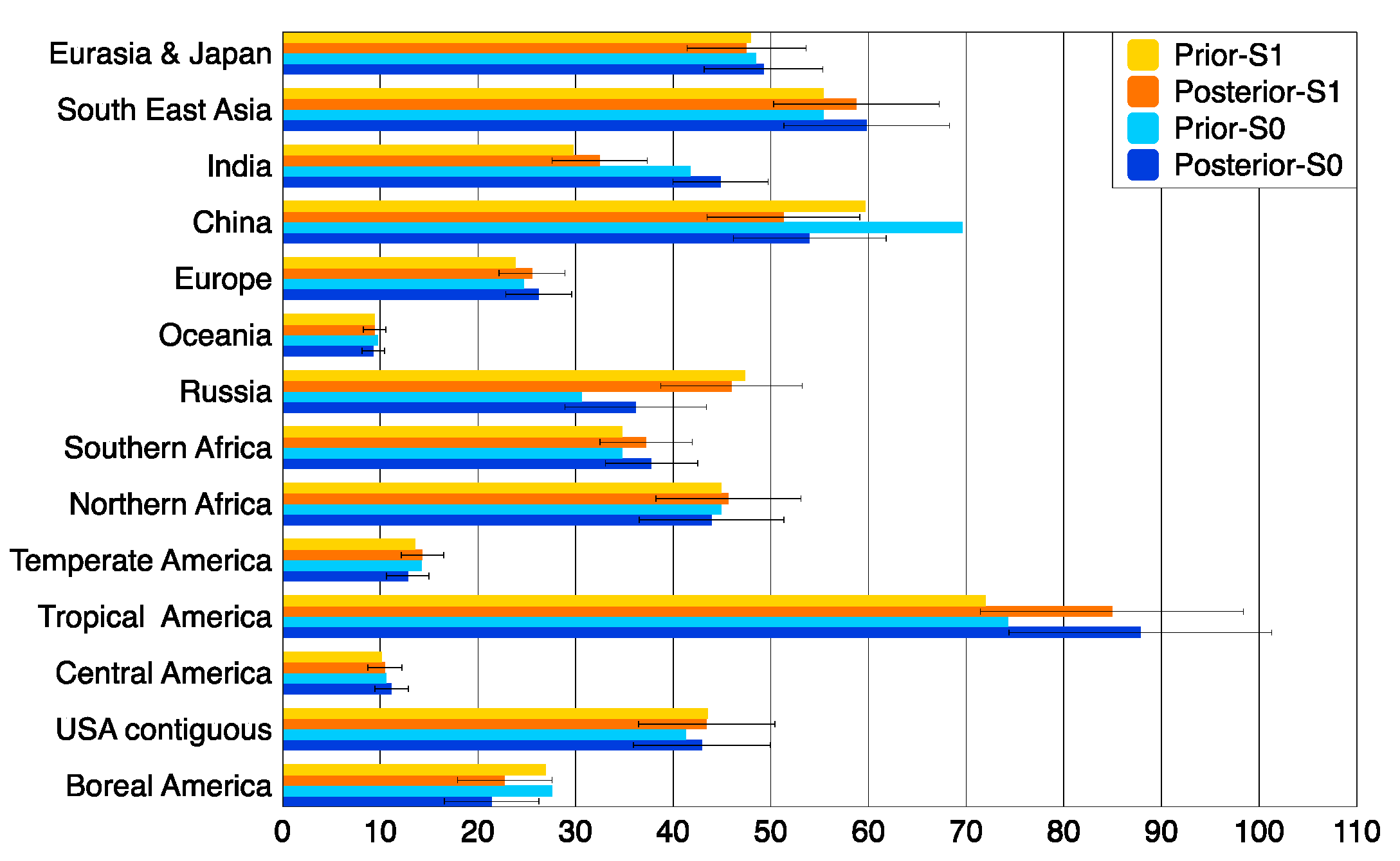
3.3.1. Total Regional Emissions

Regional methane emissions for fourteen regions are shown in Figure 3. These regions were described by Saunois et al. [10] and modified in our study by combining Taiwan with China (removing it from central Eurasia and Japan).

The inverse model-estimated corrections of total emissions were found to vary among regions, with the most significant changes taking place in Russia and India. The total methane emissions optimized by inversion for Russia increased by 27% from 36.2 to 46 Tg CH₄ yr⁻¹ when the prior anthropogenic emissions were adjusted from EDGAR to UNFCCC values (cases S0 to S1), and the inversion adjusted the emissions downwards. The reduction in the total prior methane emissions for India was 29%, and the posterior emissions decreased from 44.8 to 32.5 Tg CH₄ yr⁻¹ from case S0 to S1. Temperate South America showed 12% higher posterior emissions (from 12.8 to 14.3 Tg CH₄ yr⁻¹) and boreal North America increased by 6% (from 21.4 to 22.7 Tg CH₄ yr⁻¹), while the estimates for central North America decreased by 6% (from 11.2 to 10.5 Tg CH₄ yr⁻¹). The differences in the optimized total methane emissions for contiguous USA, Oceania, Southern Africa, Southeast Asia, and Europe were less than 3% between case S0 and S1. The optimized total methane emissions of contiguous USA slightly increased from 42.9 to 43.4 Tg CH₄ yr⁻¹ by implementing the UNFCCC scale but were still lower than the estimation by Miller et al. [23] (47.2 Tg CH₄ yr⁻¹) and Turner et al. [23] (52.4 Tg CH₄ yr⁻¹). The optimized total methane emissions for Europe decreased from 26.2 to 25.5 Tg CH₄ yr⁻¹, and these values were 6%–7% higher compared with the prior fluxes in both cases. The results are in line with the estimation (26.8 Tg CH₄ yr⁻¹) from the multi-model experiment for the EU-28 for 2006–2012 [65]. For boreal North America and China, the inverse model lowered the total methane emissions in both cases. The optimized total methane emissions for China decreased from 53.7 to 50.5 Tg CH₄ yr⁻¹, which is higher than the total methane emissions of China estimated as 38.6 Tg CH₄ yr⁻¹ in 2007 by Zhang et al. [66]. Other inverse modeling studies have also inferred smaller emissions than the EDGAR estimate for China [14,67].

3.3.2. Regional Anthropogenic Emissions

The anthropogenic methane emissions in the 14 regions are shown in Figure 4. China is the biggest emitter, reporting a 16% lower value than the UNFCCC in 2012 than the estimation of the EDGAR inventory. Our inverse modeling results are more in line with the UNFCCC reports, which reduced the estimates from 48 (S0) to 44 (S1) Tg CH₄ yr⁻¹, which is very similar to the estimation by Peng et al. [15] with 44.9 Tg CH₄ yr⁻¹ in 2010. In India, the inverse model optimized the UNFCCC emissions upwards by 25% reaching 25 Tg CH₄ yr⁻¹. This estimate is higher than that reported by Ganesan et al. [33] (22 Tg CH₄ yr⁻¹). Europe reported lower anthropogenic emissions by about 10% with the UNFCCC value compared with the EDGAR estimation, but the optimized estimates were 24.5 and 23.9 Tg CH₄ yr⁻¹—6% and 8% higher than prior emissions for cases S0 and S1, respectively. The most distinct changes were found for Russia, where the prior anthropogenic methane emissions almost doubled from 17 to 33 Tg CH₄ yr⁻¹ by implementing UNFCCC scales, and the posterior emissions also increased from 19.6 to 32 Tg CH₄ yr⁻¹. The inversion-optimized results suggest that reports to the UNFCCC by Russia may overestimate the emissions while EDGAR may underestimate them. To some extent, our estimates of the anthropogenic emissions are influenced by natural emissions, as local concentration increases can be attributed both to natural and anthropogenic sources. Better separation between these emission categories is achieved when source regions with dominant anthropogenic and natural emissions are geographically separated as they are in the USA, Western Europe, or China. The notable advantage of high-resolution simulations, which are useful for separating between emission categories, are their ability to reproduce high concentration methane plumes of anthropogenic origin significantly exceeding the signals of natural wetland emissions. Another factor contributing to separating the sources is the difference in seasonality of anthropogenic and wetland emissions (Section 3.3.1), e.g., low wetland emissions in extratropical winter.

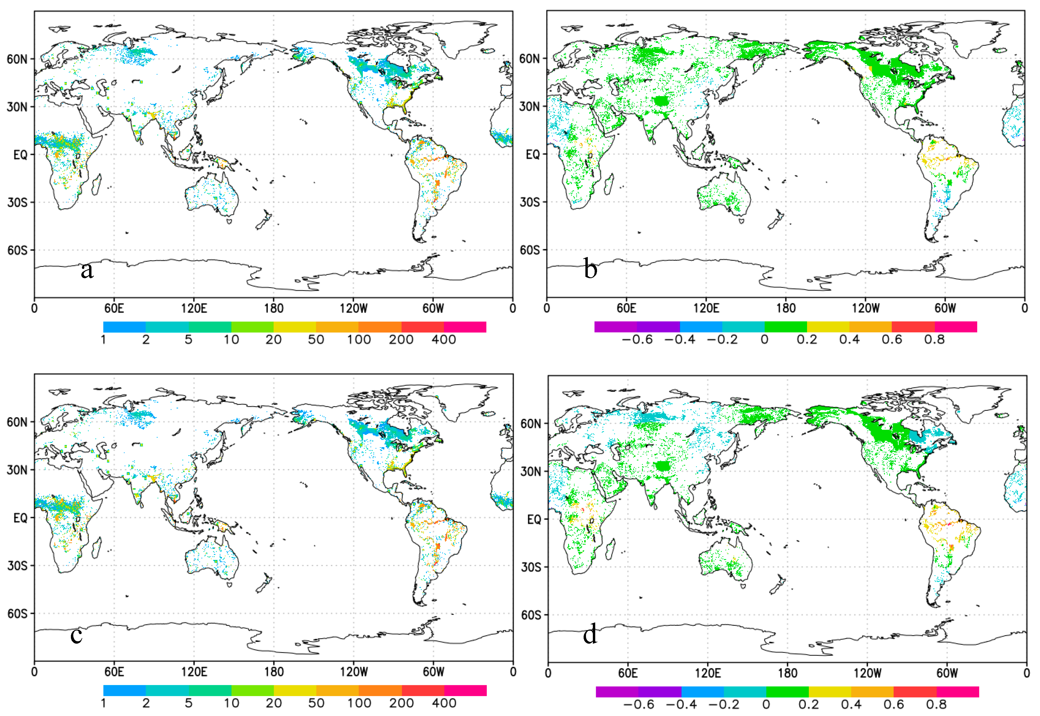
3.4. Spatial Patterns of the Flux Corrections

The anthropogenic posterior fluxes for 2010–2012 and the flux correction scales for cases with prior emissions of EDGAR (S0) and EDGAR scaled to UNFCCC reports (S1) are presented in Figure 5. The optimized anthropogenic emissions are represented by the ratios of anthropogenic corrections ($COR{R}_{an}$) to multi-annual average EDGAR emissions defined in Equation (3):

$$scal{e}_{an}=COR{R}_{an}/EDGA{R}_{2008-2012} .$$

(3)

The two optimized flux maps (2010–2012 average) for cases S0 and S1 are not distinguishable in Figure 5a,c showing large emissions in Southeast Asia, while the scaling factor maps illustrate evident differences. Figure 5b depicts obvious anthropogenic emission increases in northern Europe, Russia, and boreal America, and a larger area of decrease in east China for case S0. The scaling factor of case S1 shown in Figure 5d illustrates a relatively smaller decrease in China compared with that shown for S0, and a slight decrease in Russia. Case S1 shows a larger increase in the scaling factor over India compared that shown for S0, which is likely to be caused by lower prior emissions in case S1.

The average natural posterior fluxes for the years 2010–2012 and the scaling factors are presented in Figure 6. The optimized fluxes are represented by the ratios of wetland flux corrections ($COR{R}_w$) to the multi-annual mean VISIT prior emissions defined in Equation (4):

$$scal{e}_w=COR{R}_w/VISI{T}_{2008-2013}$$

(4)

where $scal{e}_w$ is the wetland emission scaling factor. The prior natural emissions from the VISIT emission inventory are shown to be the same for both cases (S0 and S1). The scaling factors are used to illustrate the optimization of fluxes. Figure 6d shows a greater increase in the Amazon area and greater decreases in Siberia and boreal America for case S1 compared with those shown in Figure 6b for case S0. It is shown that lower wetland emissions are required in Siberia with higher anthropogenic prior emissions for Russia in the S1 case.

3.5. Modeled Concentrations Versus Observations

The inversion results were evaluated by comparing the modeled concentrations to observations of ground-based stations and GOSAT values shown in

Table 2. Mean bias and the root-mean-square error (RMSE) for cases S0 and S1.

Case	Number of Observations	Bias (ppb)	RMSE (ppb)
S0-prior ground	89,059	−6.49	45.19
S0-posterior ground	76,772	−4.61	26.62
S1-prior ground	89,059	−5.17	44.80
S1-posterior ground	76,481	−4.24	26.40
S0-prior GOSAT	329,483	−12.30	24.39
S0-posterior GOSAT	272,101	−5.29	12.26
S1-prior GOSAT	329,483	−14.56	24.14
S1-posterior GOSAT	254,657	5.59	8.93

. Three years of observation, from 2010 to 2012, were used in each simulation, and the model outputted the forward concentrations (simulated with prior fluxes) and optimized concentrations (simulated with posterior fluxes). The bias (model minus observation data mismatch) and the root-mean-square error (RMSE) were calculated for cases S0 and S1. The bias was defined as the average mismatch between the observations and model (model minus observations) throughout the observation period. The RMSE was an aggregated form of the residuals (the difference between observed values and simulated values). Improvement of model simulation for reproducing the observations was found when changing the prior emissions from case S0 to S1. Table 2 shows that the mean RMSE decreased from prior to posterior emissions in both cases, and the optimized RMSE for GOSAT data was lower for the S1 case. RMSE was improved by flux optimization by almost half for both ground-based and GOSAT data. Additionally, the mean RMSEs and bias decreased from S0 to S1 for ground-based data.

The time series of atmospheric methane concentrations at selected stations for case S1 is shown in Figure 7, including the global background in the South-West Pacific (MLO: Mauna Loa), the regional European background (PAL: Pallas), a European mountain station in Switzerland (JFJ: Jungfraujoch), and a station influenced by anthropogenic emissions in Asia (RYO: Ryori). The optimized emissions induced better reproduction of the methane concentrations with lower RMSE values at each site.

4. Conclusions

In this paper, we have presented a comparison of the methane bottom-up emission inventories with inversion estimates using the global 0.1° × 0.1° high-resolution model NIES-TM-FLEXPART-VAR. The use of high-resolution transport helps to reduce biases in transport and inversion caused by the broadening of the anthropogenic emission plumes due to crude model resolution and numerical diffusion. EDGAR v4.3.2 provided methane emission values until 2012, and some differences in country totals can be found compared to the national reports to the UNFCCC, e.g., an underestimation of emissions by EDGAR in Russia by 50% and an overestimation by 20–40% for China and India. High resolution global inversion was employed to evaluate the effect of improved prior information using national reports with more detailed statistical data and country-specific emission factors. The original EDGAR v4.3.2 and the UNFCCC-adjusted emissions were used as two sets of anthropogenic prior emissions (for cases S0 and S1 respectively) together with biomass burning (GFASv1.2), wetlands (VISIT), and other natural sources. With the prior anthropogenic emissions adjusted from EDGAR to the UNFCCC, the total methane emissions optimized by inversion increased from 36.2 to 46 Tg CH₄ yr⁻¹ (27%) for Russia and 12.8 to 14.3 Tg CH₄ yr⁻¹ (12%) for temperate South America, and they decreased from 44.8 to 32.5 Tg CH₄ yr⁻¹ (28%) for India and 54 to 51.3 Tg CH₄ yr⁻¹ (5%) for China. The inverse corrections of total methane emissions also varied by region—upward by ~18% (of the total) for tropical South America for both S0 and S1 cases, and downward by 22% and 15% for boreal North America, and 22% and 14% for China for both S0 and S1 cases, respectively. The most insignificant corrections occurred in central Eurasia and Japan (<2% for both cases). The ratios between the average flux (2010–2012) and the multi-annual average EDGAR and VISIT fluxes were also analyzed. Case S0 showed an apparent increase in anthropogenic emissions in central Europe, Russia, and contiguous USA, and a larger area of decrease in east China compared with case S1. The natural emissions shown for case S1 showed a greater increase in the Amazon area and decreases in Siberia and boreal North America compared to those shown for case S0. The inversions were also evaluated by the comparison between modeled concentrations and observations. The advantage of using the national reports to scale EDGAR emissions was supported by achieving a better fit for both the forward and optimized model simulations to the observations with our model setup. The country scale top-down emissions should be further evaluated and advanced to provide support for the improvement of the national reports to UNFCCC.

References

1. Etheridge, D.; Steele, L.; Francey, R.; Langenfelds, R. Atmospheric methane between 1000 AD and present: Evidence of anthropogenic emissions and climatic variability. J. Geophys. Res. Atmos. 1998, 103, 15979–15993. [Google Scholar] [CrossRef]
2. Ferretti, D.; Miller, J.; White, J.; Etheridge, D.; Lassey, K.; Lowe, D.; Meure, C.; Dreier, M.; Trudinger, C.; van Ommen, T.; et al. Unexpected changes to the global methane budget over the past 2000 years. Science 2005, 309, 1714–1717. [Google Scholar] [CrossRef] [PubMed]
3. Ghosh, A.; Patra, P.; Ishijima, K.; Umezawa, T.; Ito, A.; Etheridge, D.; Sugawara, S.; Kawamura, K.; Miller, J.; Dlugokencky, E.; et al. Variations in global methane sources and sinks during 1910–2010. Atmos. Chem. Phys. 2015, 15, 2595–2612. [Google Scholar] [CrossRef]
4. Saunois, M.; Jackson, R.; Bousquet, P.; Poulter, B.; Canadell, J. The growing role of methane in anthropogenic climate change. Environ. Res. Lett. 2016, 11, 120207. [Google Scholar] [CrossRef] [Green Version]
5. Shindell, D.; Kuylenstierna, J.; Vignati, E.; van Dingenen, R.; Amann, M.; Klimont, Z.; Anenberg, S.; Muller, N.; Janssens-Maenhout, G.; Raes, F.; et al. Simultaneously Mitigating Near-Term Climate Change and Improving Human Health and Food Security. Science 2012, 335, 183–189. [Google Scholar] [CrossRef] [Green Version]
6. Zhang, Y.; Jacob, D.; Maasakkers, J.; Sulprizio, M.; Sheng, J.; Gautam, R.; Worden, J. Monitoring global tropospheric OH concentrations using satellite observations of atmospheric methane. Atmos. Chem. Phys. 2018, 18, 15959–15973. [Google Scholar] [CrossRef] [Green Version]
7. Prather, M.; Holmes, C.; Hsu, J. Reactive greenhouse gas scenarios: Systematic exploration of uncertainties and the role of atmospheric chemistry. Geophys. Res. Lett. 2012, 39. [Google Scholar] [CrossRef] [Green Version]
8. Sonnemann, G.; Grygalashvyly, M. Effective CO2 lifetime and future CO2 levels based on fit function. Ann. Geophys. 2013, 31, 1591–1596. [Google Scholar] [CrossRef]
9. Feng, T.; Yang, Y.; Xie, S.; Dong, J.; Ding, L. Economic drivers of greenhouse gas emissions in China. Renew. Sustain. Energy Rev. 2017, 78, 996–1006. [Google Scholar] [CrossRef]
10. Saunois, M.; Bousquet, P.; Poulter, B.; Peregon, A.; Ciais, P.; Canadell, J.; Dlugokencky, E.; Etiope, G.; Bastviken, D.; Houweling, S.; et al. The global methane budget 2000–2012. Earth Syst. Sci. Data 2016, 8, 697–751. [Google Scholar] [CrossRef]
11. Lyon, D.; Zavala-Araiza, D.; Alvarez, R.; Harriss, R.; Palacios, V.; Lan, X.; Talbot, R.; Lavoie, T.; Shepson, P.; Yacovitch, T.; et al. Constructing a Spatially Resolved Methane Emission Inventory for the Barnett Shale Region. Environ. Sci. Technol. 2015, 49, 8147–8157. [Google Scholar] [CrossRef] [PubMed] [Green Version]
12. Peischl, J.; Karion, A.; Sweeney, C.; Kort, E.; Smith, M.; Brandt, A.; Yeskoo, T.; Aikin, K.; Conley, S.; Gvakharia, A.; et al. Quantifying atmospheric methane emissions from oil and natural gas production in the Bakken shale region of North Dakota. J. Geophys. Res. Atmos. 2016, 121, 6101–6111. [Google Scholar] [CrossRef]
13. Saunois, M.; Bousquet, P.; Poulter, B.; Peregon, A.; Ciais, P.; Canadell, J.; Dlugokencky, E.; Etiope, G.; Bastviken, D.; Houweling, S.; et al. Variability and quasi-decadal changes in the methane budget over the period 2000–2012. Atmos. Chem. Phys. 2017, 17, 11135–11161. [Google Scholar] [CrossRef]
14. Kirschke, S.; Bousquet, P.; Ciais, P.; Saunois, M.; Canadell, J.; Dlugokencky, E.; Bergamaschi, P.; Bergmann, D.; Blake, D.; Bruhwiler, L.; et al. Three decades of global methane sources and sinks. Nat. Geosci. 2013, 6, 813–823. [Google Scholar] [CrossRef]
15. Peng, S.; Piao, S.; Bousquet, P.; Ciais, P.; Li, B.; Lin, X.; Tao, S.; Wang, Z.; Zhang, Y.; Zhou, F. Inventory of anthropogenic methane emissions in mainland China from 1980 to 2010. Atmos. Chem. Phys. 2016, 16, 14545–14562. [Google Scholar] [CrossRef] [Green Version]
16. Le Quere, C.; Andrew, R.; Friedlingstein, P.; Sitch, S.; Hauck, J.; Pongratz, J.; Pickers, P.; Korsbakken, J.; Peters, G.; Canadell, J.; et al. Global Carbon Budget 2018. Earth Syst. Sci. Data 2018, 10, 2141–2194. [Google Scholar] [CrossRef] [Green Version]
17. Oliver, J.; Bouwman, A.; Vandermass, C.; Berdowski, J. Emission database for global atmospheric research (EDGAR). Environ. Monit. Assess. 1994, 31, 93–106. [Google Scholar] [CrossRef]
18. Crippa, M.; Guizzardi, D.; Muntean, M.; Schaaf, E.; Dentener, F.; van Aardenne, J.; Monni, S.; Doering, U.; Olivier, J.; Pagliari, V.; et al. Gridded emissions of air pollutants for the period 1970–2012 within EDGAR v4.3.2. Earth Syst. Sci. Data 2018, 10, 1987–2013. [Google Scholar] [CrossRef]
19. Janssens-Maenhout, G.; Crippa, M.; Guizzardi, D.; Muntean, M.; Schaaf, E.; Dentener, F.; Bergamaschi, P.; Pagliari, V.; Olivier, J.; Peters, J.; et al. EDGAR v4.3.2 Global Atlas of the three major Greenhouse Gas Emissions for the period 1970–2012. Earth Syst. Sci. Data Discuss. 2019, 2019, 959–1002. [Google Scholar] [CrossRef]
20. Bergamaschi, P.; Krol, M.; Meirink, J.; Dentener, F.; Segers, A.; van Aardenne, J.; Monni, S.; Vermeulen, A.; Schmidt, M.; Ramonet, M.; et al. Inverse modeling of European CH4 emissions 2001–2006. J. Geophys. Res. Atmos. 2010, 115. [Google Scholar] [CrossRef]
21. Brown, M. Deduction of emissions of source gases using an objective inversion algorithm and a chemical-transport model. J. Geophys. Res. Atmos. 1993, 98, 12639–12660. [Google Scholar] [CrossRef]
22. Sheng, J.; Jacob, D.; Turner, A.; Maasakkers, J.; Sulprizio, M.; Bloom, A.; Andrews, A.; Wunch, D. High-resolution inversion of methane emissions in the Southeast US using SEAC (4) RS aircraft observations of atmospheric methane: Anthropogenic and wetland sources. Atmos. Chem. Phys. 2018, 18, 6483–6491. [Google Scholar] [CrossRef]
23. Turner, A.; Jacob, D.; Wecht, K.; Maasakkers, J.; Lundgren, E.; Andrews, A.; Biraud, S.; Boesch, H.; Bowman, K.; Deutscher, N.; et al. Estimating global and North American methane emissions with high spatial resolution using GOSAT satellite data. Atmos. Chem. Phys. 2015, 15, 7049–7069. [Google Scholar] [CrossRef] [Green Version]
24. Miller, S.; Wofsy, S.; Michalak, A.; Kort, E.; Andrews, A.; Biraud, S.; Dlugokencky, E.; Eluszkiewicz, J.; Fischer, M.; Janssens-Maenhout, G.; et al. Anthropogenic emissions of methane in the United States. Proc. Natl. Acad. Sci. USA 2013, 110, 20018–20022. [Google Scholar] [CrossRef] [PubMed] [Green Version]
25. Miller, S.; Michalak, A.; Detmers, R.; Hasekamp, O.; Bruhwiler, L.; Schwietzke, S. China’s coal mine methane regulations have not curbed growing emissions. Nat. Commun. 2019, 10, 303. [Google Scholar] [CrossRef]
26. Sheng, J.; Jacob, D.; Turner, A.; Maasakkers, J.; Benmergui, J.; Bloom, A.; Arndt, C.; Gautam, R.; Zavala-Araiza, D.; Boesch, H.; et al. 2010-2016 methane trends over Canada, the United States, and Mexico observed by the GOSAT satellite: Contributions from different source sectors. Atmos. Chem. Phys. 2018, 18, 12257–12267. [Google Scholar] [CrossRef]
27. Houweling, S.; Bergamaschi, P.; Chevallier, F.; Heimann, M.; Kaminski, T.; Krol, M.; Michalak, A.; Patra, P. Global inverse modeling of CH4 sources and sinks: An overview of methods. Atmos. Chem. Phys. 2017, 17, 235–256. [Google Scholar] [CrossRef]
28. Jacob, D.; Turner, A.; Maasakkers, J.; Sheng, J.; Sun, K.; Liu, X.; Chance, K.; Aben, I.; McKeever, J.; Frankenberg, C. Satellite observations of atmospheric methane and their value for quantifying methane emissions. Atmos. Chem. Phys. 2016, 16, 14371–14396. [Google Scholar] [CrossRef] [Green Version]
29. Shirai, T.; Ishizawa, M.; Zhuravlev, R.; Ganshin, A.; Belikov, D.; Saito, M.; Oda, T.; Valsala, V.; Gomez-Pelaez, A.; Langenfelds, R.; et al. A decadal inversion of CO2 using the Global Eulerian-Lagrangian Coupled Atmospheric model (GELCA): Sensitivity to the ground-based observation network. Tellus Ser. B Chem. Phys. Meteorol. 2017, 69, 1291158. [Google Scholar] [CrossRef]
30. Belikov, D.; Maksyutov, S.; Yaremchuk, A.; Ganshin, A.; Kaminski, T.; Blessing, S.; Sasakawa, M.; Gomez-Pelaez, A.; Starchenko, A. Adjoint of the global Eulerian-Lagrangian coupled atmospheric transport model (A-GELCA v1.0): Development and validation. Geosci. Model Dev. 2016, 9, 749–764. [Google Scholar] [CrossRef]
31. Bergamaschi, P.; Krol, M.; Dentener, F.; Vermeulen, A.; Meinhardt, F.; Graul, R.; Ramonet, M.; Peters, W.; Dlugokencky, E. Inverse modelling of national and European CH4 emissions using the atmospheric zoom model TM5. Atmos. Chem. Phys. 2005, 5, 2431–2460. [Google Scholar] [CrossRef]
32. Manning, A.; Ryall, D.; Derwent, R.; Simmonds, P.; O’Doherty, S. Estimating European emissions of ozone-depleting and greenhouse gases using observations and a modeling back-attribution technique. J. Geophys. Res. Atmos. 2003, 108. [Google Scholar] [CrossRef]
33. Ganesan, A.; Rigby, M.; Lunt, M.; Parker, R.; Boesch, H.; Goulding, N.; Umezawa, T.; Zahn, A.; Chatterjee, A.; Prinn, R.; et al. Atmospheric observations show accurate reporting and little growth in India’s methane emissions. Nat. Commun. 2017, 8, 836. [Google Scholar] [CrossRef] [PubMed]
34. Maksyutov, S.; Oda, T.; Saito, M.; Janardanan, R.; Belikov, D.; Kaiser, J.W.; Zhuravlev, R.; Ganshin, A.; Valsala, V. Technical note: High resolution inverse modelling technique for estimating surface CO2 fluxes based on coupled NIES-TM—Flexpart transport model and its adjoint. Atmos. Chem. Phys. Discuss. 2019. in preparation. [Google Scholar]
35. UNFCCC. Greenhouse Gas Inventory Data. Available online: https://di.unfccc.int/comparison_by_category (accessed on 20 November 2018).
36. Ganshin, A.; Oda, T.; Saito, M.; Maksyutov, S.; Valsala, V.; Andres, R.; Fisher, R.; Lowry, D.; Lukyanov, A.; Matsueda, H.; et al. A global coupled Eulerian-Lagrangian model and 1 × 1 km CO2 surface flux dataset for high-resolution atmospheric CO2 transport simulations. Geosci. Model Dev. 2012, 5, 231–243. [Google Scholar] [CrossRef]
37. Zhuravlev, R.V.; Ganshin, A.V.; Maksyutov, S.S.; Oshchepkov, S.L.; Khattatov, B.V. Estimation of global CO2 fluxes using ground-based and satellite (GOSAT) observation data with empirical orthogonal functions. Atmos. Ocean. Opt. 2013, 26, 507–516. [Google Scholar] [CrossRef]
38. Ishizawa, M.; Mabuchi, K.; Shirai, T.; Inoue, M.; Morino, I.; Uchino, O.; Yoshida, Y.; Belikov, D.; Maksyutov, S. Inter-annual variability of summertime CO2 exchange in Northern Eurasia inferred from GOSAT XCO2. Environ. Res. Lett. 2016, 11, 105001. [Google Scholar] [CrossRef]
39. Belikov, D.; Maksyutov, S.; Sherlock, V.; Aoki, S.; Deutscher, N.; Dohe, S.; Griffith, D.; Kyro, E.; Morino, I.; Nakazawa, T.; et al. Simulations of column-averaged CO2 and CH4 using the NIES TM with a hybrid sigma-isentropic (sigma-theta) vertical coordinate. Atmos. Chem. Phys. 2013, 13, 1713–1732. [Google Scholar] [CrossRef]
40. Stohl, A.; Forster, C.; Frank, A.; Seibert, P.; Wotawa, G. Technical note: The Lagrangian particle dispersion model FLEXPART version 6.2. Atmos. Chem. Phys. 2005, 5, 2461–2474. [Google Scholar] [CrossRef] [Green Version]
41. Hascoet, L.; Pascual, V. The Tapenade Automatic Differentiation Tool: Principles, Model, and Specification. ACM Trans. Math. Softw. 2013, 39, 20. [Google Scholar] [CrossRef]
42. Giering, R.; Kaminski, T. Applying TAF to generate efficient derivative code of Fortran 77–95 programs. Proc. Appl. Math. Mech. 2003, 2, 54–57. [Google Scholar] [CrossRef]
43. Van Leer, B. Towards the ultimate conservative difference scheme. V. A second-order sequel to Godunov’s method. J. Comput. Phys. 1997, 135, 229–248. [Google Scholar] [CrossRef]
44. Onogi, K.; Tslttsui, J.; Koide, H.; Sakamoto, M.; Kobayashi, S.; Hatsushika, H.; Matsumoto, T.; Yamazaki, N.; Kaalhori, H.; Takahashi, K.; et al. The JRA-25 reanalysis. J. Meteorol. Soc. Jpn. 2007, 85, 369–432. [Google Scholar] [CrossRef]
45. Kobayashi, S.; Ota, Y.; Harada, Y.; Ebita, A.; Moriya, M.; Onoda, H.; Onogi, K.; Kamahori, H.; Kobayashi, C.; Endo, H.; et al. The JRA-55 Reanalysis: General Specifications and Basic Characteristics. J. Meteorol. Soc. Jpn. 2015, 93, 5–48. [Google Scholar] [CrossRef] [Green Version]
46. Meirink, J.; Bergamaschi, P.; Krol, M. Four-dimensional variational data assimilation for inverse modelling of atmospheric methane emissions: Method and comparison with synthesis inversion. Atmos. Chem. Phys. 2008, 8, 6341–6353. [Google Scholar] [CrossRef]
47. Basu, S.; Guerlet, S.; Butz, A.; Houweling, S.; Hasekamp, O.; Aben, I.; Krummel, P.; Steele, P.; Langenfelds, R.; Torn, M.; et al. Global CO2 fluxes estimated from GOSAT retrievals of total column CO2. Atmos. Chem. Phys. 2013, 13, 8695–8717. [Google Scholar] [CrossRef]
48. Weaver, A.; Courtier, P. Correlation modelling on the sphere using a generalized diffusion equation. Q. J. R. Meteorol. Soc. 2001, 127, 1815–1846. [Google Scholar] [CrossRef]
49. Press, W.H.; Flannery, B.P.; Teukolsky, S.A.; Vetterling, W.T. Numerical Recipes in FORTRAN 77, 2nd ed.; Cambridge University Press: Cambridge, UK, 1992; p. 1010. [Google Scholar]
50. Gilbert, J.; Lemarechal, C. Some numerical experiments with variable-storage quasi-newton algorithms. Math. Program. 1989, 45, 407–435. [Google Scholar] [CrossRef]
51. Cao, M.; Marshall, S.; Gregson, K. Global carbon exchange and methane emissions from natural wetlands: Application of a process-based model. J. Geophys. Res. Atmos. 1996, 101, 14399–14414. [Google Scholar] [CrossRef] [Green Version]
52. Curry, C. Modeling the soil consumption of atmospheric methane at the global scale. Glob. Biogeochem. Cycles 2007, 21. [Google Scholar] [CrossRef]
53. Ito, A.; Inatomi, M. Use of a process-based model for assessing the methane budgets of global terrestrial ecosystems and evaluation of uncertainty. Biogeosciences 2012, 9, 759–773. [Google Scholar] [CrossRef] [Green Version]
54. Lehner, B.; Doll, P. Development and validation of a global database of lakes, reservoirs and wetlands. J. Hydrol. 2004, 296, 1–22. [Google Scholar] [CrossRef]
55. Running, S.; Nemani, R.; Heinsch, F.; Zhao, M.; Reeves, M.; Hashimoto, H. A continuous satellite-derived measure of global terrestrial primary production. Bioscience 2004, 54, 547–560. [Google Scholar] [CrossRef]
56. Kaiser, J.W.; Heil, A.; Andreae, M.O.; Benedetti, A.; Chubarova, N.; Jones, L.; Morcrette, J.-J.; Razinger, M.; Schultz, M.G.; Suttie, M.; et al. Biomass burning emissions estimated with a global fire assimilation system based on observed fire radiative power. Biogeosciences 2012, 9, 527–554. [Google Scholar] [CrossRef] [Green Version]
57. Patra, P.; Houweling, S.; Krol, M.; Bousquet, P.; Belikov, D.; Bergmann, D.; Bian, H.; Cameron-Smith, P.; Chipperfield, M.; Corbin, K.; et al. TransCom model simulations of CH4 and related species: Linking transport, surface flux and chemical loss with CH4 variability in the troposphere and lower stratosphere. Atmos. Chem. Phys. 2011, 11, 12813–12837. [Google Scholar] [CrossRef]
58. Yoshida, Y.; Kikuchi, N.; Morino, I.; Uchino, O.; Oshchepkov, S.; Bril, A.; Saeki, T.; Schutgens, N.; Toon, G.; Wunch, D.; et al. Improvement of the retrieval algorithm for GOSAT SWIR XCO2 and XCH4 and their validation using TCCON data. Atmos. Meas. Tech. 2013, 6, 1533–1547. [Google Scholar] [CrossRef]
59. Chevallier, F.; Breon, F.; Rayner, P. Contribution of the Orbiting Carbon Observatory to the estimation of CO2 sources and sinks: Theoretical study in a variational data assimilation framework. J. Geophys. Res. Atmos. 2007, 112. [Google Scholar] [CrossRef]
60. Olivier, J.G.J.; Jeroen, A.H.W. Trends in Global CO2 and Total Greenhouse Gas Emissions; PBL Publishers: Sydney, Australia, 2018; Available online: https://www.pbl.nl/en/publications/trends-in-global-co2-and-total-greenhouse-gas-emissions-2018-report (accessed on 11 January 2019).
61. Hoglund-Isaksson, L. Bottom-up simulations of methane and ethane emissions from global oil and gas systems 1980 to 2012. Environ. Res. Lett. 2017, 12, 024007. [Google Scholar] [CrossRef]
62. IPCC. Carbon and Other Biogeochemical Cycles. In ClimateChange 2013: The Physical Science Basis; Stocker, T.F., Qin, D., Plattner, G.K., Tignor, M., Allen, S.K., Boschung, J., Nauels, A., Xia, Y., Bex, V., Midgley, P.M., Eds.; Cambridge University Press: Cambridge, UK; New York, NY, USA, 2013. [Google Scholar]
63. Ribeiro, I.; Andreoli, R.; Kayano, M.; de Sousa, T.; Medeiros, A.; Guimaraes, P.; Barbosa, C.; Godoi, R.; Martin, S.; de Souza, R. Impact of the biomass burning on methane variability during dry years in the Amazon measured from an aircraft and the AIRS sensor. Sci. Total Environ. 2018, 624, 509–516. [Google Scholar] [CrossRef]
64. Ishizawa, M.; Chan, D.; Worthy, D.; Chan, E.; Vogel, F.; Maksyutov, S. Analysis of atmospheric CH4 in Canadian Arctic and estimation of the regional CH4 fluxes. Atmos. Chem. Phys. 2019, 19, 4637–4658. [Google Scholar] [CrossRef]
65. Bergamaschi, P.; Karstens, U.; Manning, A.; Saunois, M.; Tsuruta, A.; Berchet, A.; Vermeulen, A.; Arnold, T.; Janssens-Maenhout, G.; Hammer, S.; et al. Inverse modelling of European CH4 emissions during 2006–2012 using different inverse models and reassessed atmospheric observations. Atmos. Chem. Phys. 2018, 18, 901–920. [Google Scholar] [CrossRef]
66. Zhang, B.; Chen, G. Methane emissions in China 2007. Renew. Sustain. Energy Rev. 2014, 30, 886–902. [Google Scholar] [CrossRef]
67. Bergamaschi, P.; Houweling, S.; Segers, A.; Krol, M.; Frankenberg, C.; Scheepmaker, R.; Dlugokencky, E.; Wofsy, S.; Kort, E.; Sweeney, C.; et al. Atmospheric CH4 in the first decade of the 21st century: Inverse modeling analysis using SCIAMACHY satellite retrievals and NOAA surface measurements. J. Geophys. Res. Atmos. 2013, 118, 7350–7369. [Google Scholar] [CrossRef]
Figure 1. Comparison of anthropogenic methane emissions (units: Tg CH4 yr−1) between national reports to the UNFCCC and EDGAR v4.3.2 (G1: group 1, G2: group 2, and G3: group 3). The top emitting countries (based on the amount of emissions in the year 2012) are presented.
Remotesensing 11 02489 g001
Figure 2. (a) Monthly variation in global total methane emissions (tot) and anthropogenic emissions (an), (b) monthly variation in wetland emissions (vss) and anthropogenic emissions. S0: simulation with EDGAR v4.3.2 and S1: simulation with EDGAR v4.3.2 scaled to UNFCCC reports.
Remotesensing 11 02489 g002
Figure 3. Regional total methane emissions (unit Tg CH4 yr−1) in 2010–2012 for cases S0 and S1. Error bars are the posterior uncertainties.
Remotesensing 11 02489 g003
Figure 4. Regional anthropogenic methane emissions (unit Tg CH4 yr−1) in 2010–2012 for cases S0 and S1. The error bars are the estimation uncertainties.
Remotesensing 11 02489 g004
Figure 5. Posterior anthropogenic methane fluxes (S0 (a) and S1 (c)) and scaling factors (S0 (b) and S1 (d)). (2010–2012 average, unit mg CH4 m−2 day−1).
Remotesensing 11 02489 g005
Figure 6. Posterior natural methane fluxes (S0 (a) and S1 (c)) and scaling factors (S0 (b) and S1 (d)). (2010–2012 average, unit mg CH4 m−2 d−1).
Remotesensing 11 02489 g006
Figure 7. Observations, prior (forward), and posterior (optimized) modeled concentrations at selected sites in 2010. Mean bias and root-mean-square error (RMSE) values for each site are shown. (JFJ: 7.99E, 46.55N; MLO: 155.58W, 19.54N; PAL: 24.07E, 67.58N; and RYO: 144.32E, 39.03N).
Remotesensing 11 02489 g007