Application for Terrestrial LiDAR on Mudstone Erosion Caused by Typhoons


Department of Geography, National Taiwan University, Taipei 10617, Taiwan
*
Author to whom correspondence should be addressed.
Remote Sens. 2019, 11(20), 2425; https://doi.org/10.3390/rs11202425
Submission received: 28 August 2019
/
Revised: 17 October 2019
/
Accepted: 17 October 2019
/
Published: 18 October 2019
(This article belongs to the Special Issue Point Cloud Processing and Analysis in Remote Sensing)
Abstract
:Storms are important agents for shaping the Earth’s surface and often dominate the landscape evolution of mudstone areas, by rapid erosion and deposition. In our research, we used terrestrial scanning LiDAR (TLS) to detect surface changes in a 30 m in height, 60 m in width mudstone slope. This target slope shows the specific erosion pattern during extreme rainfall events such as typhoons. We investigate two major subjects: (1) how typhoon events impact erosion in the target slope, and (2) how rills develop on the hillslopes during these observation periods. There were three scans obtained in 2011, and converted to two observation periods. The permanent target points (TP) method and DEMs of differences were used to check the accuracy of point cloud. The results showed that the average erosion rate was 5 cm during the dry period in 2011. Following the typhoons, the erosion rate increased 1.4 times to 7 cm and was better correlated with the increase in the rainfall intensity than with general precipitation amounts. The hillslope gradient combined with rainfall intensity played a significant role in the geomorphic process. We found that in areas with over 75° gradients with larger rainfall intensity showed more erosion that at other gradients. The gradient also influenced the rill development, which occurred at middle and low gradients but not at high gradients. The rills also created a transition zone for erosion and deposition at the middle gradient where a minimal change occurred.

1. Introduction
Mudstone shows heterogeneous erodibility in response to soil moisture, especially during extreme rainfall events, because extreme rainfall can increase its water content in a short time, i.e., mudstone is a clay-bearing material and its characteristic allows rapid weathering and erosion [1,2]. Taiwan, an island with an area of 36,000 km2, has 30% of its area in the southwest part composed of mudstone. This mudstone area accounts for up to 0.1% of the high sediment discharge in the world [3] and creates dynamic landscapes during humid weather [4].
The tipping point of mudstone erosion is the wet–dry circle, resulting in slake [5,6,7] and shrinking due to drying-out in the dry season [8,9,10]. This process produces mud cracks and surface crusts that both develop soil piping, rills, and gullies [11,12,13]. According to these events, mudstone slopes can more dynamically change than other mother-rock materials during rainfall events and become a battered field for slope erosion processes.
Compared with flat ground, slopes can more potentially experience erosion because of their gradient, especially for mudstone materials. Slope erosions are initiated by gravity and rainfall [14,15,16,17,18]. Additionally, the effects of slope gradient, slope erosion [19,20,21,22], gullies, rills [16,23,24], and their interactions [14,25,26] are well documented. However, the interrelationship between typhoons and rill erosion have, until now, not been well investigated. The mudstone slope, which can rapidly change, provides a natural sandbox for observation of geomorphic process within a human lifetime.
LiDAR is a survey method to measure the distance between target and device by counting the flying time of laser signal. It can measure wild range target and are convenient compared with other methods, e.g., real time response and digital model building, low cost, better mobility, can operate in dark, and determine physical and chemical composition by the reflecting laser wavelanth [27]. Comparing the classical methods using in erosion research, such as erosion pins and sediment traps [28,29,30], high spatial-resolution topography data obtained from airborne LiDAR and terrestrial scanning LiDAR (TLS) provide precise and detailed landscape changes, e.g., terrain analysis [31], landslide [32,33,34,35], rockfall [36,37,38], beach erosion [39], channel erosion [40,41,42], and slope erosion [43,44,45,46]. This research is helpful for studying the geomorphological processes in a certain spatial scale where traditional tools can hardly reach, and provide more evidence of landscape evolution.
The present study aims to:
- provide a series of quantitative surface changes after typhoon events,
- linkage erosion pattern, rainfall intensity, and hillslope gradient cause by typhoon events. We use TLS to scan a 1007 m2 hillslope. Based on the TLS results, we focused on the erosion rate and erosion pattern affected by precipitation.
2. Material and Methods
2.1. Location
The location for this study was Tenliao, north of Kaoshung City, Taiwan. This area is located on a mudstone formation called Gutinkan (Figure 1). This formation is composed of fine mud that forms a shallow sea bottom and raised by tectonic movement [47]. According to the geological map [48], the average thickness of this mudstone formation is approximately 1 km. The mudstone content there is rich in cations (especially sodium). Inside this formation, there are corals and sandstone layers encapsulated by mudstone. In addition, one active normal fault exists nearby to the east of the study area. However, even though the study area was located at the same upper plate no fault activity occurred during the study period [49,50], and this fault did not affect our field observations.
The target slope there is a single hill, with dimensions 60 m wide, 30 m high and 1007 m2 of area (Figure 2). The shadow-relief image shows that this slope has high-relief change by the ridge of sub slopes, and the extended area at the foot of the slope is limited by an artificial plate (Figure 2a). The gradient image shows that the slope degree of most area is 40° or higher instead of the slope feet (Figure 2b). This slope is made up of mudstone, and has the classic scene for concentrated rills coming out of a drainage map (Figure 2c).
2.2. Climate
The climate is tropical monsoon, and the annual rainfall is approximately 2000 mm. However, rainfall amounts are distinctly different between seasons. More than 87% of the annual rainfall events are concentrated between June and October [51]. During the remainder of the year, hot and dry weather prevails. In the rainy season for our location, high intensity rainfall events are primarily caused by typhoons. They can bring large amounts precipitation in a short period of time (rainfall intensity), which generates the strong forces that cause erosion due to rainfall and runoff. This also weakens the mudstone due to the shrinking–slaking cycle of its clay component. Taiwan may see three or four typhoons each year, each of which causes runoff, enhances with each storm that brings large amounts of rain and increases the rate of erosion.
2.3. TLS for Data Acquisition
We chose Leica ScanStation 2 as the TLS equipment. This scanner is based on the time-of-flight principle and provides spatial resolution up to a centimeter for landscape monitoring. This scanner can obtain 50,000 points in second with green beam laser class 3R. The scanning range is up to 300 m@90 albedo reflecitivity. The accuracy of single measurement by scanner are 6 mm for position detecting, 4 mm for distance, and 60 μrad for Angle at 1–50 m. The spot size is 4 mm(from 0–50 m) and 6 mm (from 50–300 m). The point spacing is fully selectable horizontal and vertical with 1 mm minimum spacing though the full range. The modeled surface precision is 2 mm (1 sigma) in stand distance (50 m), according to the original factory specification [52]. The operating program of the scanner is the software Leica Cyclone 7.4, provided by the manufacturer. In addition, the software can be used as a tool for registration function and laying out of the final position.
During the measurement periods (dry and humid), the scanner was placed at similar locations in front of the target slope. The project grid of slope scanning is 0.01 m × 0.01 m. We fixed the data for each period to the same grid using 10 benchmarks around the target area. The first, second, and third point clouds were acquired on 24 February, 27 May, and 4 August 2011. The total number of scanning points for each scans were around two million (Table 1). To reduce the shadow area blocked by the local relief [53], all scanning results were co-registered using at least six scans at different positions.
2.4. DEM Processing
We converted the point cloud to digital elevation models (DEMs) and classified the rest of their changes as erosion [46]. In the first step, the quality of DEMs must be validated. The quality of DEMs depends on the technical abilities of the scanner, and the strategy of the field survey. Error and accurary estimating is an issue for scanning data [54,55,56]. In this case, we use the application of the method of permanent target points (TP). The TP method is based on a network of permanent target points, which obtains georeferencing by GPS and INS. When operating the scanner, the position of targets will be recognized by the software (Leical Cyclone 7.4), and identify them by manual selection [57,58,59]. We use the circle target on the benchmarks as ti-points around the target slope, and obtained their georeferencing information by Leica TPS 1101 total station. These points join into other temporary ti-points in the scan data. The Leica Cyclone program ortho-calibrated all point clouds into the same local grid system and obtained the first calibration error during constraint processing (<0.6 cm in all control points) (Table 2). In addition, we used the georeferencing information of benchmarks (control points) to check the errors producing by two grid systems (TLS and local position system). The root mean square (RMS) of ti-points shows the error of all three scans less than 0.005 m. The DEMs of difference (DoD) [60] of two periods are 0.00336 m (first periods) and 0.00297 m (second periods).
After the cloud calibration and incorporation in each of the scans, the subsequent process used the Leica Cyclone program to convert the data from point clouds to DEM. The original point cloud data could only be managed by the Leica Cyclone 7.4 with its unique format, and this software suffers from the limitation in terms of collaboration with other software, e.g., the lars and grid (geo-tiff) format. However, we choose ArcGIS and MATLAB as the analyzing tools with grid data. Due to the format limitation of Leica Cyclone 7.4, we exported the point cloud to txt files with an xyz spatial structure, then input ArcGis by creating the xyz events, and finally converted to grid format (geo-tiff) for MATLAB.
More than six million measured points from three scans were converted into point-shape file from Cyclone by using ArcGIS 10.5. To set the ideal grid size of DEMs, which can capture points with evenly distribution. The high relief of target slope strongly affect the spatial distribution of the scanning points, and thus it caused some areas to have low point density, even to be blank.
To reduce the blank area of the grid and maintain the accuracy of the measured points, we needed to introduce the measured points into each cell to be as few as possible. The best condition was for each cell to contain only one point. Therefore, calculating the correlation between the point cloud and cell size was necessary. A 2 cm × 2 cm cell size contained almost one sampling point and satisfied the precondition, i.e., it should be larger than 1.6 cm × 1.6 cm. We selected the “Point to Grid” function of ArcGIS 10.5 to capture the scanning points in the grid, and this grid covered 90% of the target slope surface. Blank zones appeared in the shadow areas located under the relief similar to the borders between the sub-slope systems. However, the follow-up analysis required data that covered the entire slope area. Thus, we used the inverse distance weighting method to interpolate the three DEMs to 10 cm × 10 cm, which covered all target slope surfaces without a blank and still retained the topography characteristics.
2.5. DEM Data Analyzing
To clarify the relationship among erosion, gradient, and drainage area, we used the DEMs to calculate the height change using three observations. Height change was defined as the difference in the DEMs, which represented the median and standard deviation of the erosion. The gradient was calculated according to its fineness degree. The drainage area was filled from the high to low gradient at every 10 m2. In addition, we also plotted the difference in the DEMs in the slope area as a topographical map to illustrate the characteristics of the erosion and deposition, which could help distinguish the effect due to the rills.
2.6. Rainfall
There were two observation periods from 24 February–27 May, and 27 May–4 August 2011. Two typhoons, namely Meari, and Ma-on, occurred from 23–25 June and 15–18 July 2011, respectively (Table 3). To understand the effect of the typhoon events, we needed to clarify the rainfall distribution in three periods: dry season (without typhoon events), rainfall season (with typhoon events), and long-term conditions. Here, we focused on the volume of precipitation and rainfall intensity. The rainfall records were obtained from the nearest official rainfall station Guting (maintained by the central weather bureau), which recorded hourly weather information from 1992 to 2016.
In the first period (February to May 2011), the record showed that the total rainfall was 170 mm over 51 h in 91 days. Most of the rainfall were less than 10 mm, and only one hourly rainfall reached 80 mm. The second period (May to August 2011) was an extended rainy season with many rainfall events. The record showed that the total precipitation accumulated up to 800 mm over 170 h, especially with the occurrence of two heavy rainfall events related to typhoons where levels reached up to 222 and 307.5 mm.
Figure 3 shows the rainfall probability in the two periods and the long-term record of the weather station, and the second period similar to the long-term period. In the first period (Figure 3a), the graph shows that the highest intensity was only 20 mm/h with no probability of rainfall beyond the normal intensity. Rainfall with weak intensity did not generate deep stream flow for erosion. In the second period (Figure 3b), the curve shows that the maximum rainfall intensity extended up to 40 mm/h and had almost the same probability of middle-intensity rainfall. For the long-term data (Figure 3c), the graph was different from the first but similar to the second period. The maximum rainfall intensity was approximately 40 mm/h and exhibited a smoother curve from middle to low rainfall intensity. The second period could represent a long-term rainfall situation. The first period demonstrated only a one-half rainfall intensity compared with the second period and with the long-term rainfall situation because of the lack of precipitation.
3. Results
After comparing the DEMs of different scans, we obtained the numbers of topographical change of the target slope in two periods (Table 4). In first periods, the erosion rate was 5.09 cm, depended on the lower net erosion and higher depositon. In contrast, second periods had erosion rate 7.745 cm by higher erosion and lower deposition. Compared with the second period, the change in the erosion rate (1.6×) is much closer to the change in the maximum rainfall erosion (2.0×) than the total precipitation. For a more detailed explaination of topographical change, we separated three parts to discriptthe: erosion classification (the relationship between erosion volume, drainage area and gradient) (Figure 4); erosion volume according to the different gradients (the link between erosion volume and gradient) (Figure 5); and the erosion pattern (erosion on the slope) (Figure 6).
3.1. Erosion Classification
The picture of relationship among the hillslope gradient, height change, and drainage area shows the erosion place has changed in two periods (Figure 4). The first period experienced 170 mm precipitation from 24 February to 27 May 2011. In this period (Figure 4a), the erosion pattern could be classified into three parts according to the hillslope gradient. The high-gradient area (55–80°) included the slope head and ridges, which had the smallest area. The erosion was significant, with the maximum erosion depth approaching 0.3 m. The area of the middle gradient (25–55°), increased very quickly and in contrast to the high-gradient area with erosion only, both erosion and accumulation occurred in this area. The erosion in this middle-gradient area was concentrated in the upper part, and the erosion depth was less than 0.1 m. In contrast, the accumulation in the lower area experienced an approximately 0.1 m bulk increase. However, some eroded areas also became an accumulation area, which meant that they had become a transition zone between erosion and accumulation. The erosion took place at a high-relief area such as the boundary and head of the rills. Accumulation occurred in relatively smooth areas in the rill channel and flat surfaces in the slope. The low-gradient areas (below 25°) were located at the downward side and toe of the target slope, which were the largest area in the study and mostly dominated by deposition. The areas experienced bulk accumulation of 0.2 m. Erosion can be seen in few areas and only above 15°.
During the second period of study (28 May to 4 August) the precipitation depth was 800 mm. This period (Figure 4b), was dominated by erosion and differences in the height change of the slope surface were caused by its gradient. In the highest gradient areas, the largest amounts of erosion occurred at the slope head, with very little change until the medium gradient area. There the height reduction due to erosion was significant at more than 0.3 m. Accumulation still occurred in these areas although at a smaller scale because rainfall intensity increased runoff, which transported the surface material farther down the hill rather than being deposited. The transition zone here was prone to erosion and transport instead of maintaining a balance. The largest increase in erosion occurred in the low-gradient areas of the slope. Here, the changes were dominated by erosion, and no measurable material was deposited. The increasing runoff provided by the rainfall intensity was more dominant here, which not only transported materials from the upper part throughout the slope system but also caused more erosion at the foot of the slope.
3.2. Erosion Volume According to the Different Gradients
Figure 5 shows various surface erosions in the target slope gradients of the two periods. In the first period (Figure 5a), the graph indicates that the erosion could be classified into three parts: slope head, middle area, and low area. In the slope head, the top area did not experience significant erosion. However, when the gradient decreased to 85–75°, a large loss occurred and caused peak erosion. From this gradient and downward to 60°, the erosion was very light and tapered off to almost nothing. In the middle-gradient area of 60–30°, erosion remained approximately 0.0 m, and the mean was maintained in the same shape. This area had also the smallest change zone from 30–50°, which was consistent with the deposition in the high-gradient area shown in Figure 3a. In the low-gradient area from 30° to the bottom, the curve reveals that deposition occurred here. The height change shifted to accumulation, and the bulk increased with the decrease in the gradient.
In the second period (Figure 5b), at first glance, the curve appears to change only in the low-gradient area. However, in reality, it shifted in the second period at all gradient degrees. Compared with the first period, the high-gradient area (from the slope head to 75°) remained an erosion-filled zone and the largest erosion volume occurred at approximately 80°. Similarly, the slope head also experienced more erosion in this period. At the middle-gradient area, the curve of the height change remained the same shape but was a few centimeters lower. However, the variation in the curvature was smaller than that in the first period. This indicates that the height of the actual slope started to decrease but kept its original shape. In the low-gradient area (from 30° to the slope bottom), an obvious difference in the curve can be seen. It shifted from deposition to erosion, and the erosion becomes more significant with the decrease in the gradient. We considered that the precipitation transformed into a surface flow, which increased the flow energy and eroded the slope due to its length and the rills. Figure 4b shows the same phenomenon at the foot of the slope.
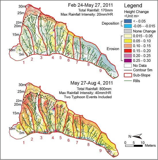
3.3. Erosion Pattern
Figure 6 shows that this study broke down the target slope to nine sub-slopes and shows the detailed erosion situations in the two periods. We found that the rills exhibited a linear geomorphic change on the slope surface according to the linear shape, especially in the second period. In the low rainfall-intensity period (Figure 6a), mudstone erosion occurred under a different condition relative to the location. In this part, the higher sub-slopes, namely Slopes 2–5, experienced maximum erosion in their slope head, which had a loss of 0.1–0.2 m. This area was 20 to 30 m high and higher than the rills could reach. Thus, the erosion assumed a belt form without a linear branch extension. The other areas experienced a mixture of no change to 0.1 m erosion. The erosion occurred in all sub-slopes below 20 m high. In these parts, the erosion zone exhibited a linear form. In the large sub-slopes, the erosion was distributed from the slope end to a height of 22 m with a linear shape. In the small sub-slopes, the erosion only occurred at the path of the rills, and other sub-slopes did not change.
In the high intensity rainfall period (Figure 6b), significant erosion occurred in the slope, and some erosion-filled zones appeared in the rills. Compared with the period of high intensity rainfall, no erosion occurred in the slope head, although a 0.1 m loss occurred. At the middle part of the slope, larger erosion from 0.15 to 0.3 m occurred. At the foot of the slope, light erosion occurred with a 0.1 m loss. Across these two parts, the rills exhibited the largest erosion of up to 0.3 m. The linear shape of rills extended to the foot of the slope and included the slope end where 0.3 m erosion also occurred but accompanied with deposition. The rills accumulated more runoff to generate stronger energy, which caused more erosion and transported the surface materials. Some materials were deposited at the slope end, but some of them were flushed outside the slope system by the rills. Thus, both significant erosion and deposition occurred.
4. Discussion
4.1. Influence of Rainfall Intensity
The rainfall intensity exhibited better correlation with the topographical change than the total rainfall (Table 4). The brief steady level of rainfall record in the two periods indicated that the second period had more erosion energy that changed the mudstone hillslope. To clarify the relationship of these two factors, we needed to check if other possible factors affected the erosion, such as earthquake. During the observation periods, no big earthquake and human activities occurred. Therefore, rainfall would most likely be responsible for the topographical change during the two periods. To trigger slope erosion, precipitation must exceed the erosion threshold. The erosion threshold for a mudstone badland is 10 mm/h [61], Thus, we filtered out some small-rainfall events (6%) and reduced the probabilities of slope erosion. In addition, the erosion areas were designated to be with those with high gradient because steepness exerts more effect on soil loss than rainfall intensity [62]. In the low-gradient area, small erosion occurred and even shifted to a deposition-dominated area. Therefore, the low rainfall intensity in the first period caused little erosion because the soil could absorb the rain.
The high rainfall intensity caused by the two typhoon events boosted the topographical development in the second period. The rainfall intensity greatly affected the energy for soil erosion [63]. Compared with the change due to a low rainfall intensity, the erosion everywhere was significant. However, the topographical changes from the slope head to the slope end were not consistent. The erosion could be classified into three categories according to the degree of height change, and they appeared to be related with the gradient. We considered that the rainfall intensity was a trigger that controlled the erosion degree. High rainfall intensity increased the erosion volume at the slope surface, but the detail of the topographical change was dominated by another factor.
4.2. Importance of Slope Gradient
Figure 3 shows that the slope could be classified into three parts according to their reactions under rainfall intensity. They even exhibited unique change characteristics for erosion or deposition. Some of their topographical conditions were the same, especially the range of their gradients. We considered that the gradient controlled their reactions under different rainfall intensities.
First, the erosion increased with the increase in the gradient in the slope-head area. However, Figure 5a shows that rills did not significantly develop in high-gradient areas, such as the slope head. They stopped at the lower edge of the erosion-filled zone at approximately 60°. Considering that rills could not develop at high gradients, the erosion there must be caused by surface-stream flow and raindrops. In addition, the edge area was also the border of two erosion types because of the relative higher gradient.
The rills joined the erosion process when the slope gradient decreased to 60°. When the rills broke apart, some places experienced mixed erosion and deposition. The evidence is shown in Figure 5a. Some rills had a linear shape as a rill path starting from the border to the hillslope bottom. These rills did not experience much erosion with runoff but deposition. The rills eroded materials from its upper part or in the inter-rill area and then transported them to the slope bottom. These sediments became the main source of deposition [64,65,66,67]. In this case, the gradient influenced the type of erosion processes that occurred [68]. which caused different erosion conditions.
Another complex event took place in the second period under a high rainfall intensity, as shown in Figure 3b and Figure 5b. Because the typhoons brought high rainfall density, not only did significant erosion occur from the slope head to the middle-gradient area but also the low-gradient area experienced a shift from deposition to erosion. The high rainfall intensity boosted the raindrop and stream flow in the slope head and enhanced rill development from the middle to the lower parts of the slope. Thus, they reduced the slope surface [14,67]. The rills eroded materials from the upper part or inter-rill area and then transported them to the slope bottom. These sediments became the main source of deposition during the low rainfall intensity. When the intensity became high, additional water flowed, which made the rills more active, caused additional erosion, and transported the eroded materials outside the slope system. This phenomenon in the second period was in contrast to that in the first period and created large erosion at the low-gradient area.
The middle part of the target slope experienced the smallest effect of erosion in both two periods. Even when rills were developed and caused erosion somewhere, the topographical change was not critical. Figure 4 shows that the curve of the erosion slightly shifted under different rainfall intensities, but the variation in the erosion at each successive gradient was very close to reveal almost the same height loss. This phenomenon created a stable zone at certain degrees. In this zone, the erosion and deposition were balanced by the material transported through the high-gradient area and thus mitigated the soil loss. When the gradient decreased, the condition also changed with the rainfall intensity to cause either erosion or deposition. We called this zone as a transition zone for the erosion or deposition process.
4.3. Applications of High-Resolution Topography in Slope Erosion
As a progressively developed technique, TLS provides low-cost (time and laboratory energy consumption) advantages with high-spatial-resolution DEMs. In contrast to pervious methods, landscape monitoring were mostly applied to estimate vertical offsets using leveling measurements, aerial survey, and field observations, i.e., gully erosion [69], earthquake induced landslides [70], and badland erosion in Spain [66].
Our TLS results demonstrated the feasibility of topographical analysis in a tiny scale landscape. The morphological features can be more efficiently and flexibly conducted from DEMs than aerial LiDAR method [71]. Accordingly, we suggest that TSL can obtain precise information about erosion from any space within the slope, especially the local topographic gradient and erosion depth, to investigate the morphologic phenomenon (Figure 4).
In addition, these results would extend the comprehensiveness of the interaction of the erosional processes and rainfall intensity on mudstone slopes, and also provide guidance for further landscape-evolution prediction using a physical model. We need to note that TLS analysis using highly erodible material is a good method of observing the effect of weather events to explain the processes of slope evolution.
High-spatial-resolution datasets surveyed using TLS fulfills its potential when applied to topography changing studies [32,34,38,40]. According to the findings of the present study, we suggest that the DEMs obtained from TLS can powerfully detect surface changes owing to their data quality and field convenience, particularly for landscape monitoring.
5. Conclusions
This study used TLS to survey the surface erosion of mudstone slope caused by typhoon events. The results show that the average erosion rate of the target slope was 0.05 m during the dry season in 2011. After the typhoon events, the average erosion during the rainfall season increased up to 0.07 m, especially in areas more than 22-m high. Compared with the precipitation, the increase in the erosion rate appeared to have better correlation with the increase in the rainfall intensity because of the high gradient. When extreme precipitation occurred, the high rainfall intensity could enhance erosion to trigger topographical changes in the target slope.
The hillslope gradient played a more important role than the rainfall intensity on the topographical change. The target slope could be classified into three zones according to certain gradients. Each of the zones showed different erosion and deposition activities. The slope-head zone experienced the same activity under different intensities. However, the middle and downslope zones were affected by rills, especially during the rainy season with two typhoon events. The precipitation due to the typhoons triggered significant erosion along the rill path and transported slope materials outside the slope system.
TLS provided a large contribution to this research owing to its high spatial and time resolution. We believed that TLS can perform topography monitoring, particularly in research on tiny spatial scale.
Author Contributions
Conceptualization, Y.-C.C. and C.-J.Y.; methodology, Y.-C.C. and C.-J.Y.; investigation, Y.-C.C.; writing—original draft preparation, Y.-C.C.; writing—review, C.-J.Y.; editing, Y.-C.C. and C.-J.Y.; supervision, J.-C.L.
Funding
This research was funded by MOST of Taiwan, grant number NSC 101-2116-M-002-011-.
Acknowledgments
We would like to thank MOST of Taiwan for the research.
Conflicts of Interest
The authors declare no conflict of interest.
References
- Gautam, T.P.; Shakoor, A. Slaking behavior of clay-bearing rocks during a one-year exposure to natural climatic conditions. Eng. Geol. 2013, 166, 17–25. [Google Scholar] [CrossRef]
- Gautam, T.P.; Shakoor, A. Comparing the Slaking of Clay-Bearing Rocks Under Laboratory Conditions to Slaking Under Natural Climatic Conditions. Rock Mech. Rock Eng. 2016, 49, 19–31. [Google Scholar] [CrossRef]
- Dadson, S.J.; Hovius, N.; Chen, H.G.; Dade, W.B.; Hsieh, M.L.; Willett, S.D.; Hu, J.C.; Horng, M.J.; Chen, M.C.; Stark, C.P.; et al. Links between erosion, runoff variability and seismicity in the Taiwan orogen. Nature 2003, 426, 648–651. [Google Scholar] [CrossRef] [PubMed]
- Chen, C.T.A.; Ae, C.; Liu, J.; Tsuang, B.J. Island-based catchment—The Taiwan example. Reg. Environ. Chang. 2004, 4, 39–48. [Google Scholar] [CrossRef]
- Baets, S.D.; Torri, D.; Poesen, J.; Salvador, M.P.; Meersmans, J. Modelling increased soil cohesion due to roots with EUROSEM. Earth Surf. Process. Landf. 2008, 33, 1948–1963. [Google Scholar] [CrossRef]
- Zhang, C.L.; Wieczorek, K.; Xie, M.L. Swelling experiments on mudstones. J. Rock Mech. Geotech. Eng. 2010, 2, 44–51. [Google Scholar] [CrossRef]
- Zhang, D.; Chen, A.; Xiong, D.; Liu, G. Effect of moisture and temperature conditions on the decay rate of a purple mudstone in southwestern China. Geomorphology 2013, 182, 125–132. [Google Scholar] [CrossRef]
- Kikumoto, M.; Putra, A.D.; Fukuda, T. Slaking and deformation behaviour. Geotechnique 2016, 66, 771–785. [Google Scholar] [CrossRef]
- Sharma, K.; Kiyota, T.; Kyokawa, H. Effect of slaking on direct shear behaviour of crushed mudstones. Soils Found. 2017, 57, 288–300. [Google Scholar] [CrossRef]
- Hu, M.; Liu, Y.X.; Ren, J.B.; Zhang, Y.; Song, L.B. Temperature-induced slaking characteristics of mudstone during dry-wet cycles. Int. J. Heat Technol. 2017, 35, 339–346. [Google Scholar] [CrossRef]
- Yamasaki, S.; Chigira, M. Weathering mechanisms and their effects on landsliding in pelitic schist. Earth Surf. Process. Landf. 1993, 494, 481–494. [Google Scholar] [CrossRef]
- Sass, O. Rock moisture measurements: Techniques, results, and implications for weathering. Earth Surf. Process. Landf. 2005, 30, 359–374. [Google Scholar] [CrossRef]
- Battaglia, S.; Leoni, L.; Rapetti, F.; Spagnolo, M. Dynamic evolution of badlands in the Roglio basin (Tuscany, Italy). Catena 2011, 86, 14–23. [Google Scholar] [CrossRef]
- Bouchnak, H.; Felfoul, M.S.; Boussema, M.R.; Snane, M.H. Slope and rainfall effects on the volume of sediment yield by gully erosion in the Souar lithologic formation (Tunisia). Catena 2009, 78, 170–177. [Google Scholar] [CrossRef]
- Hattanji, T.; Moriwaki, H. Morphometric analysis of relic landslides using detailed landslide distribution maps: Implications for forecasting travel distance of future landslides. Geomorphology 2009, 103, 447–454. [Google Scholar] [CrossRef] [Green Version]
- Ghimire, S.K.; Higaki, D.; Bhattarai, T.P. Gully erosion in the Siwalik Hills, Nepal: Estimation of sediment production from active ephemeral gullies. Earth Surf. Process. Landf. 2006, 31, 155–165. [Google Scholar] [CrossRef]
- Owen, J.J.; Amundson, R.; Dietrich, W.E.; Nishiizumi, K.; Sutter, B.; Chong, G. The sensitivity of hillslope bedrock erosion to precipitation. Earth Surf. Process. Landf. 2011, 36, 117–135. [Google Scholar] [CrossRef]
- Berger, C.; Schulze, M.; Rieke-Zapp, D.; Schlunegger, F. Rill development and soil erosion: A laboratory study of slope and rainfall intensity. Earth Surf. Process. Landf. 2010, 35, 1456–1467. [Google Scholar] [CrossRef]
- Chaplot, V. Impact of terrain attributes, parent material and soil types on gully erosion. Geomorphology 2013, 186, 1–11. [Google Scholar] [CrossRef]
- Chaplot, V.; Bissonnais, Y.L.E.; Sol, S.; Recherche, C.D. Field measurements of interrill erosion under different slopes and plot sizes. Earth Surf. Process. Landf. 2000, 153, 145–153. [Google Scholar] [CrossRef]
- Ribolzi, O.; Patin, J.; Bresson, L.M.; Latsachack, K.O.; Mouche, E.; Sengtaheuanghoung, O.; Silvera, N.; Thiebaux, J.P.; Valentin, C. Impact of slope gradient on soil surface features and infiltration on steep slopes in northern Laos. Geomorphology 2011, 127, 53–63. [Google Scholar] [CrossRef]
- Bou Kheir, R.; Chorowicz, J.; Abdallah, C.; Dhont, D. Soil and bedrock distribution estimated from gully form and frequency: A GIS-based decision-tree model for Lebanon. Geomorphology 2008, 93, 482–492. [Google Scholar] [CrossRef]
- Descroix, L.; González Barrios, J.L.; Viramontes, D.; Poulenard, J.; Anaya, E.; Esteves, M.; Estrada, J. Gully and sheet erosion on subtropical mountain slopes: Their respective roles and the scale effect. CATENA 2008, 72, 325–339. [Google Scholar] [CrossRef]
- Hancock, G.R.; Evans, K.G. Gully, channel and hillslope erosion–an assessment for a traditionally managed catchment. Earth Surf. Process. Landf. 2010, 35, 1468–1479. [Google Scholar] [CrossRef]
- Fang, H.; Sun, L.; Tang, Z. Effects of rainfall and slope on runoff, soil erosion and rill development: An experimental study using two loess soils. Hydrol. Process. 2015, 29, 2649–2658. [Google Scholar] [CrossRef]
- Tian, P.; Xu, X.Y.; Pan, C.Z.; Hsu, K.L.; Yang, T.T. Impacts of rainfall and inflow on rill formation and erosion processes on steep hillslopes. J. Hydrol. 2017, 548, 24–39. [Google Scholar] [CrossRef]
- Barbarella, M.; Fiani, M. Monitoring of large landslides by Terrestrial Laser Scanning techniques: Field data collection and processing. Eur. J. Remote Sens. 2013, 46, 126–151. [Google Scholar] [CrossRef]
- Clarke, M.L.; Rendell, H.M. Process-form relationships in Southern Italian badlands: Erosion rates and implications for landform evolution. Earth Surf. Process. Landf. 2006, 31, 15–29. [Google Scholar] [CrossRef]
- Della Seta, M.; Del Monte, M.; Fredi, P.; Lupia Palmieri, E. Space–time variability of denudation rates at the catchment and hillslope scales on the Tyrrhenian side of Central Italy. Geomorphology 2009, 107, 161–177. [Google Scholar] [CrossRef]
- Fang, N.F.; Zeng, Y.; Ni, L.S.; Shi, Z.H. Estimation of sediment trapping behind check dams using high-density electrical resistivity tomography. J. Hydrol. 2019, 568, 1007–1016. [Google Scholar] [CrossRef]
- Gillin, C.P.; Bailey, S.W.; McGuire, K.J.; Prisley, S.P. Evaluation of Lidar-derived DEMs through Terrain Analysis and Field Comparison. Photogramm. Eng. Remote Sens. 2015, 81, 387–396. [Google Scholar] [CrossRef] [Green Version]
- Teza, G.; Galgaro, A.; Zaltron, N.; Genevois, R. Terrestrial laser scanner to detect landslide displacement fields: A new approach. Int. J. Remote Sens. 2007, 28, 3425–3446. [Google Scholar] [CrossRef]
- Teza, G.; Pesci, A.; Genevois, R.; Galgaro, A. Characterization of landslide ground surface kinematics from terrestrial laser scanning and strain field computation. Geomorphology 2008, 97, 424–437. [Google Scholar] [CrossRef]
- Baldo, M.; Bicocchi, C.; Chiocchini, U.; Giordan, D.; Lollino, G. LIDAR monitoring of mass wasting processes: The Radicofani landslide, Province of Siena, Central Italy. Geomorphology 2009, 105, 193–201. [Google Scholar] [CrossRef]
- Bitelli, G.; Dubbini, M.; Zanutta, A. Terrestrial laser scanning and digital photogrammetry techniques to monitor landslide bodies. Int. Arch. Photogramm. Remote Sens. Spat. Inf. Sci. 2004, 35, 246–251. [Google Scholar]
- Abellan, A.; Vilaplana, J.M.; Martinez, J. Application of a long-range Terrestrial Laser Scanner to a detailed rockfall study at Vall de Nuria (Eastern Pyrenees, Spain). Eng. Geol. 2006, 88, 13. [Google Scholar] [CrossRef]
- Abellán, A.; Calvet, J.; Vilaplana, J.M.; Blanchard, J. Detection and spatial prediction of rockfalls by means of terrestrial laser scanner monitoring. Geomorphology 2010, 119, 162–171. [Google Scholar] [CrossRef]
- Abellán, A.; Oppikofer, T.; Jaboyedoff, M.; Rosser, N.J.; Lim, M.; Lato, M.J.; Ne, T. Terrestrial laser scanning of rock slope instabilities. Earth Surf. Process. Landf. 2013, 97, 80–97. [Google Scholar] [CrossRef]
- Corbi, H.; Riquelme, A.; Megias-Banos, C.; Abellan, A. 3-D Morphological Change Analysis of a Beach with Seagrass Berm Using a Terrestrial Laser Scanner. ISPRS Int. Geo. Inf. 2018, 7, 234. [Google Scholar] [CrossRef]
- Milan, D.J.; Heritage, G.L.; Hetherington, D. Application of a 3D laser scanner in the assessment of erosion and deposition volumes and channel change in a proglacial river. Earth Surf. Process. Landf. 2007, 32, 1657–1674. [Google Scholar] [CrossRef]
- Schwendel, A.C.; Fuller, I.C.; Death, R.G. Assessing DEM interpolation methods for effective representation of upland stream morphology for rapid appraisal of bed stability. River Res. Appl. 2012, 28, 567–584. [Google Scholar] [CrossRef]
- Vaaja, M.; Hyyppä, H.; Kukko, A.; Kaartinen, H.; Alho, P. Mapping Topography Changes and Elevation Accuracies Using a Mobile Laser Scanner. Remote Sens. 2011, 3, 587–600. [Google Scholar] [CrossRef] [Green Version]
- Usmanov, B.; Yermolaev, O.; Gafurov, A. Estimates of slope erosion intensity utilizing terrestrial laser scanning. Proc. Int. Assoc. Hydrol. Sci. 2015, 367, 59–65. [Google Scholar] [CrossRef]
- Nadal-Romero, E.; Revuelto, J.; Errea, P.; López-Moreno, J.I. The application of terrestrial laser scanner and SfM photogrammetry in measuring erosion and deposition processes in two opposite slopes in a humid badlands area (central Spanish Pyrenees). SOIL 2015, 1, 561–573. [Google Scholar] [CrossRef] [Green Version]
- Neugirg, F.; Kaiser, A.; Schmidt, J.; Becht, M.; Haas, F. Quantification, analysis and modeling of soil erosion on steep slopes using LiDAR and UAV photographs. Proc. Int. Assoc. Hydrol. Sci. 2014, 367, 51–58. [Google Scholar]
- Neugirg, F.; Kaiser, A.; Huber, A.; Heckmann, T.; Schindewolf, M.; Schmidt, J.; Becht, M.; Haas, F. Using terrestrial LiDAR data to analyse morphodynamics on steep unvegetated slopes driven by different geomorphic processes. CATENA 2016, 142, 269–280. [Google Scholar] [CrossRef]
- Sun, C.H.; Chang, S.C.; Kuo, C.L.; Wu, J.C.; Shao, P.H.; Oung, J.N. Origins of Taiwan’s mud volcanoes: Evidence from geochemistry. J. Asian Earth Sci. 2010, 37, 105–116. [Google Scholar] [CrossRef]
- Central Geological Survey, M. Geologic Map of Taiwan: Qishan Sheet, Scale 1:50,000; Central Geological Survey: New Taipei City, Taiwan, 2013.
- Pathier, E.; Fruneau, B.; Doin, M.P.; Liao, Y.T.; Hu, J.C.; Champenois, J. What are the tectonic structures accommodating the present-day tectonic deformation in South-Western Taiwan? A new interpretation from ALOS-1 InSAR and GPS interseismic measurements. In Proceedings of the Geodynamics and Environment in East-Asia: 7th France-Taiwan Earth Sciences Symposium, Hualien, Taiwan, 12–18 November 2014; pp. 12–15. [Google Scholar]
- Champenois, J.; Fruneau, B.; Pathier, E.; Deffontaines, D.; Lin, K.C.; Hu, J.C. Monitoring of active tectonic deformations in the Longitudinal Valley (Eastern Taiwan) using Persistent Scatterer InSAR method with ALOS PALSAR data. Earth Planet. Sci. Lett. 2012, 337, 12. [Google Scholar] [CrossRef]
- Chen, C.S.; Chen, Y.L. The Rainfall Characteristics of Taiwan. Mon. Weather Rev. 2003, 131, 1323–1341. [Google Scholar] [CrossRef]
- Leica-Geosystems, Leica ScanStation 2 Datasheet. Available online: https://w3.leica-geosystems.com/downloads123/hds/hds/ScanStation/brochures-datasheet/Leica_ScanStation%202_datasheet_en.pdf (accessed on 11 September 2019).
- Schaefer, M.; Inkpen, R. Towards a protocol for laser scanning of rock surfaces. Earth Surf. Process. Landf. 2010, 35, 147–423. [Google Scholar] [CrossRef]
- Huising, E.J.; Gomes Pereira, L.M. Errors and accuracy estimates of laser data acquired by various laser scanning systems for topographic applications. ISPRS J. Photogramm. Remote Sens. 1998, 53, 245–261. [Google Scholar] [CrossRef]
- Wheaton, J.M.; Brasington, J.; Darby, S.E.; Sear, D.A. Accounting for uncertainty in DEMs from repeat topographic surveys: Improved sediment budgets. Earth Surf. Process. Landf. 2010, 35, 136–156. [Google Scholar] [CrossRef]
- Lane, S.N.; Westaway, R.M.; Murray Hicks, D. Estimation of erosion and deposition volumes in a large, gravel-bed, braided river using synoptic remote sensing. Earth Surf. Process. Landf. 2003, 28, 249–271. [Google Scholar] [CrossRef]
- Kociuba, W.; Kubisz, W.; Zagórski, P. Use of terrestrial laser scanning (TLS) for monitoring and modelling of geomorphic processes and phenomena at a small and medium spatial scale in Polar environment (Scott River—Spitsbergen). Geomorphology 2014, 212, 84–96. [Google Scholar] [CrossRef]
- Kociuba, W. Analysis of geomorphic changes and quantification of sediment budgets of a small Arctic valley with the application of repeat TLS surveys. Z. Fur Geomorphol. Suppl. Issues 2017, 61, 105–120. [Google Scholar] [CrossRef]
- Kociuba, W. Assessment of sediment sources throughout the proglacial area of a small Arctic catchment based on high-resolution digital elevation models. Geomorphology 2017, 287, 73–89. [Google Scholar] [CrossRef]
- Williams, R. DEMs of difference. Geomorphol. Tech. 2012, 2, 1–17. [Google Scholar]
- Yair, A.; Bryan, R.B.; Lavee, H.; Schwanghart, W.; Kuhn, N.J. The resilience of a badland area to climate change in an arid environment. Catena 2013, 106, 12–21. [Google Scholar] [CrossRef]
- Römkens, M.J.M.; Helming, K.; Prasad, S.N. Soil erosion under different rainfall intensities, surface roughness, and soil water regimes. Catena 2002, 46, 103–123. [Google Scholar] [CrossRef]
- Wischmeier, W.H.; Smith, D.D. Rainfall energy and its relationship to soil loss. Eos Trans. Am. Geophys. Union 1958, 39, 285–291. [Google Scholar] [CrossRef]
- Kirkby, M.J.; Bracken, L.J. Gully processes and gully dynamics. Earth Surf. Process. Landf. 2009, 34, 1841–1851. [Google Scholar] [CrossRef]
- Le Roux, J.J.; Sumner, P.D. Factors controlling gully development: Comparing continuous and discontinuous gullies. Land Degrad. Dev. 2012, 23, 440–449. [Google Scholar] [CrossRef]
- Desir, G.; Marin, C. Role of erosion processes on the morphogenesis of a semiarid badland area. Bardenas Reales (NE Spain). Catena 2013, 106, 83–92. [Google Scholar] [CrossRef]
- Lee, D.H.; Chen, P.Y.; Wu, J.H.; Chen, H.L.; Yang, Y.E. Method of mitigating the surface erosion of a high-gradient mudstone slope in southwest Taiwan. Bull. Eng. Geol. Environ. 2013, 72, 533–545. [Google Scholar] [CrossRef]
- Liu, B.; Nearing, M.A.; Risse, L.M. Slope gradient effects on soil loss for steep slopes. Trans ASAE 1994, 37, 1835–1840. [Google Scholar] [CrossRef]
- Peter, K.D.; d’Oleire-Oltmanns, S.; Ries, J.B.; Marzolff, I.; Hssaine, A.A. Soil erosion in gully catchments affected by land-levelling measures in the Souss Basin, Morocco, analysed by rainfall simulation and UAV remote sensing data. Catena 2014, 113, 24–40. [Google Scholar] [CrossRef]
- Lin, J.C.; Petley, D.; Jen, C.H.; Koh, A.; Hsu, M.L. Slope movements in a dynamic environment—A case study of Tachia River, Central Taiwan. Quat. Int. 2006, 147, 103–112. [Google Scholar] [CrossRef]
- De Sy, V.; Schoorl, J.M.; Keesstra, S.D.; Jones, K.E.; Claessens, L. Landslide model performance in a high resolution small-scale landscape. Geomorphology 2013, 190, 73–81. [Google Scholar] [CrossRef] [Green Version]
Figure 1.
Location of the study area and geological boundary. The star sign shows the study area located in the Gutinkan formation, which shows it as layer t.
Figure 1.
Location of the study area and geological boundary. The star sign shows the study area located in the Gutinkan formation, which shows it as layer t.

Figure 2.
Study area map. The shadow-relief image of target slope (a), gradient image (b), and drainage map (c) created by digital elevation model.
Figure 2.
Study area map. The shadow-relief image of target slope (a), gradient image (b), and drainage map (c) created by digital elevation model.

Figure 3.
Distribution of the probability of rainfall intensity in three periods. The subpanels indicate the following: (a) 24 February–26 May 2011, representing the first period; (b) 26 May–3 August 2011, representing the second period; and 1991–2018, representing the last 28 years.
Figure 3.
Distribution of the probability of rainfall intensity in three periods. The subpanels indicate the following: (a) 24 February–26 May 2011, representing the first period; (b) 26 May–3 August 2011, representing the second period; and 1991–2018, representing the last 28 years.

Figure 4.
Relationship among the hillslope gradient, height change, and drainage area. The subpanels indicate the following: (a) 24 February–26 May 2011, representing the first period; (b) 26 May–3 August 2011, representing the second period.
Figure 4.
Relationship among the hillslope gradient, height change, and drainage area. The subpanels indicate the following: (a) 24 February–26 May 2011, representing the first period; (b) 26 May–3 August 2011, representing the second period.

Figure 5.
Changes in the erosion depth along the slope gradient in the two periods. The dots and error bars denote the median and standard deviation of the erosion-depth change in each gradient, respectively. (a) 24 February–27 May 2011. (b) 27 May–3 August 2011.
Figure 5.
Changes in the erosion depth along the slope gradient in the two periods. The dots and error bars denote the median and standard deviation of the erosion-depth change in each gradient, respectively. (a) 24 February–27 May 2011. (b) 27 May–3 August 2011.

Figure 6.
Erosion pattern in the first period (a) and second period (b) in 2011.


Table 1.
The results of three ground scans in 2011.
| Date | Project Grid Size | Number of Points | Density of Points |
|---|---|---|---|
| 2011/02/24 | 0.01m × 0.01m | 1.80 M pt | 1787.49 pt/m2 |
| 2011/05/27 | 0.01m × 0.01m | 1.94 M pt | 1926.51 pt/m2 |
| 2011/08/04 | 0.01m × 0.01m | 2.42 M pt | 2403.18 pt/m2 |
Table 2.
Registration errors of 2011 scans.
| Scan World | Target ID | Mean Absolute Error | Error Vector | RMS by Ti-Point [m] | DEMs of Differences (DoD) [m] | ||
|---|---|---|---|---|---|---|---|
| X [m] | Y [m] | Z [m] | |||||
| 2011/02/24 | TL01 | 0.001 | −0.001 | 0.000 | 0.000 | 0.004 | First period 0.00336 |
| TL02 | 0.003 | 0.003 | 0.000 | 0.000 | |||
| TL03 | 0.002 | 0.001 | 0.001 | −0.001 | |||
| TL04 | 0.003 | 0.003 | 0.000 | 0.000 | |||
| 2011/05/27 | TL01 | 0.003 | 0.001 | 0.000 | 0.003 | 0.002 | |
| TL02 | 0.004 | −0.003 | 0.001 | −0.001 | |||
| TL03 | 0.001 | 0.000 | 0.000 | −0.001 | Second period 0.00297 | ||
| TL04 | 0.002 | 0.002 | −0.001 | −0.001 | |||
| 2011/08/04 | TL01 | 0.001 | 0.000 | 0.000 | 0.000 | 0.005 | |
| TL02 | 0.001 | −0.001 | −0.001 | 0.000 | |||
| TL07 | 0.002 | −0.002 | 0.000 | 0.000 | |||
| TL11 | 0.003 | 0.002 | −0.002 | −0.001 | |||
| TL022 | 0.001 | 0.000 | −0.001 | −0.001 | |||
Table 3.
Precipitation record of the study area during the two periods in 2011. Two typhoon events bring more precipitation and higher rainfall intensity in the second period. The rainfall threshold to trigger erosion is 10 mm/day.
Table 3.
Precipitation record of the study area during the two periods in 2011. Two typhoon events bring more precipitation and higher rainfall intensity in the second period. The rainfall threshold to trigger erosion is 10 mm/day.
| Period | Date | Total Precipitation | Duration | Highest Rainfall Intensity | Typhoon |
|---|---|---|---|---|---|
| First | 02/23~05/27 | 170mm | 51 hr | 20 mm/h | None |
| Second | 05/27~08/04 | 800 mm (222mm by Meari, 307mm by Ma-on) | 170 hr | 40 mm/h | Meari and Ma-on |
Table 4.
Degree of erosion factors in the frist (February 24–May 26, 2011) and second (May 26–August 03, 2011) periods.
Table 4.
Degree of erosion factors in the frist (February 24–May 26, 2011) and second (May 26–August 03, 2011) periods.
| Period | Net Erosion (m3) | Erosion Rate (m3/m2) | Net Deposition (m3) | Total Rainfall (mm) | Max Rainfall Intensity (mm/h) |
|---|---|---|---|---|---|
| Frist | −56.4495 | −0.050983 | 28.1664 | 170 | 20 |
| Second | −94.5597 | −0.07745 | 16.9932 | 800 | 40 |
© 2019 by the authors. Licensee MDPI, Basel, Switzerland. This article is an open access article distributed under the terms and conditions of the Creative Commons Attribution (CC BY) license (http://creativecommons.org/licenses/by/4.0/).
Share and Cite
MDPI and ACS Style
Cheng, Y.-C.; Yang, C.-J.; Lin, J.-C. Application for Terrestrial LiDAR on Mudstone Erosion Caused by Typhoons. Remote Sens. 2019, 11, 2425. https://doi.org/10.3390/rs11202425
AMA Style
Cheng Y-C, Yang C-J, Lin J-C. Application for Terrestrial LiDAR on Mudstone Erosion Caused by Typhoons. Remote Sensing. 2019; 11(20):2425. https://doi.org/10.3390/rs11202425
Chicago/Turabian StyleCheng, Yeuan-Chang, Ci-Jian Yang, and Jiun-Chuan Lin. 2019. "Application for Terrestrial LiDAR on Mudstone Erosion Caused by Typhoons" Remote Sensing 11, no. 20: 2425. https://doi.org/10.3390/rs11202425
Note that from the first issue of 2016, this journal uses article numbers instead of page numbers. See further details here.