Bidirectional Convolutional LSTM Neural Network for Remote Sensing Image Super-Resolution

Abstract

Single-image super-resolution (SR) is an effective approach to enhance spatial resolution for numerous applications such as object detection and classification when the resolution of sensors is limited. Although deep convolutional neural networks (CNNs) proposed for this purpose in recent years have outperformed relatively shallow models, enormous parameters bring the risk of overfitting. In addition, due to the different scale of objects in images, the hierarchical features of deep CNN contain additional information for SR tasks, while most CNN models have not fully utilized these features. In this paper, we proposed a deep yet concise network to address these problems. Our network consists of two main structures: (1) recursive inference block based on dense connection reuse of local low-level features, and recursive learning is applied to control the model parameters while increasing the receptive fields; (2) a bidirectional convolutional LSTM (BiConvLSTM) layer is introduced to learn the correlations of features from each recursion and adaptively select the complementary information for the reconstruction layer. Experiments on multispectral satellite images, panchromatic satellite images, and nature high-resolution remote-sensing images showed that our proposed model outperformed state-of-the-art methods while utilizing fewer parameters, and ablation studies demonstrated the effectiveness of a BiConvLSTM layer for an image SR task.

1. Introduction

In the field of remote sensing, high-resolution (HR) images contain many detailed textures and critical information, which are essential for object classification and detection tasks. Under the limitation of hardware such as chips and sensors and the high production costs, super-resolution (SR) is regarded as one of the most effective approaches to obtain high spatial resolution images from single or multiple low-resolution (LR) images [1,2]. In the multi-frame method, establishing the relation between a targeted HR image and several LR images of the same scene acquired at different condition is used to create a higher resolution result. However, single-image SR algorithms have to solely rely on one given input image, which is crucial when there is no additional data available. Single-image SR methods can be efficiently used as pre-processing operations for additional manual or automatic processing steps, such as classification or object extraction in general. However, with the loss of high-frequency detailed information and multiple targets for a single LR image, the SR task is an ill-posed inverse problem.

The detail of a physical object that a conventional optical system can reproduce in an image has the limitations imposed by diffraction on the resolving power of optical systems. Harris [3] and Goodman [4] established the theoretical foundation for the SR problem by introducing the theorems of how to solve the diffraction problem in an optical system and introduced the term of SR to use as a single LR image to reconstruct HR images. In the case of imaging objects with optical fields propagating to the far-field, the basic constraint is the diffraction of light, which limits the conventional optical system to a spatial resolution comparable to the wavelength of light. Optical diffraction by the imaging system transforms all radiation sources into blurred spatial distributions. In the field of remote sensing, a point of the HR domain is blurred in the LR space during the acquisition process, which is specified as the point spread function (PSF). Hence, SR can be seen as the inverting process of the degradation generated by the imaging system to obtain an HR image. Tsai and Huang [5] proposed the idea of using multiframe LR images for reconstruction to improve the spatial resolution of Landsat TM images. A variety of approaches for remotely sensed images can be categorized as optics-based methods, interpolation methods, and machine-learning methods [6,7,8,9]. Optics-based methods such as dielectric cube terajet generation, wide-aperture lens, and solid-immersion technique have been proposed for enhancing the resolution of imaging systems [10,11,12,13,14]. Compared with optics-based methods, the idea behind machine-learning methods is to learn the potential relationships between low-resolution and high-resolution domains from an external training set, then to generate the final super-resolved image using this prior knowledge and machine-learning methods can improve the reconstruction quality in parallel with optics-based methods. Deep learning methods have achieved great performance over others among these machine-learning methods. Dong et al. [15] first proposed SRCNN with three layers of neural networks to learn the end-to-end mapping between the LR and HR patches.

Recently, many methods (e.g., VDSR [16], EDSR [17], WDSR [18]) based on very deep neural networks outperformed the relatively shallow CNN model [15,19,20]. It can be observed that among these methods, there are two main strategies for the design of the SR model as shown in Figure 1.

However, the deeper CNN model (by adding more convolutional layers) gives rise to enormous parameters and the difficulty of the training procedure. The increasing depths of neural networks by adding more convolutional layers result in overwhelming parameters and the risk of overfitting [21]. As very deep networks with enormous parameters are highly likely to overfit and demand more storage space, DRCN [22] and DRRN [23] used recursive learning to repeatedly apply the same convolutional layer or residual units to reduce the model parameters and make the model compact. To address these problems, various techniques have been introduced in SR neural networks. We mainly review these techniques under three groups shown in Figure 2.

Since there is a high correlation between the input image and the target HR image, many methods such as VDSR [2], EDSR [16], WDSR [17], SRResNet [25], SRDCN [26], and DRRN [27] use the local residual path from ResNet [24] and the global residual path to propagate the information from the shallow layer to the final reconstruction layer. Several methods based on DenseNet [27] like SRDenseNet [28] and RDN [29] use a concatenation strategy to combine preceding features to a bottleneck layer for reconstruction. MemNet [30], CARN [31], RDN [29], ESRGAN [32], and DBPN [33] also adopt dense connection to alleviate vanishing gradients and reuse the features from shallow layers. To control the parameters while achieving a large receptive field, DRCN [22] repeatedly applied the same convolutional layer at 16-recursions to reach a receptive field of 41 by 41. The DRRN [23] proposes a recursive block consisting of several residual units and shares the weights among these residual units to further improve its performance.

In the SR task, recurrent neural networks are usually implied in video SR to capture the long-term dependency from neighboring frames [34]. BRCN [35,36] consists of three parts: The feedforward convolutional layer to capture the spatial dependence between LR and HR, the bidirectional recurrent convolutional network to capture the temporal dependency between successive frames, and the conditional convolutional layer to further capture spatial-temporal dependency. STCN [37] proposes a bidirectional LSTM structure to capture spatial-temporal information for video frame reconstruction. For single image SR, based upon the idea of viewing a ResNet as an unrolled RNN [38,39], DSRN [40] proposes a dual-state recurrent network, and each state operates at the LR and HR spatial resolution separately to explore the connection between the LR and HR pairs and provides information flow from LR to HR at every recursion.

In the remote sensing area, Hua et al. [41] proposed a novel RNN model for hyperspectral image classification which can effectively analyze hyperspectral pixels as sequential data. Convolutional LSTM was utilized to address the spectral-spatial feature learning problem and extract more discriminative and abstract features for hyperspectral image classification [42,43,44]. Besides that, Mou et al. [45] proposed a recurrent convolutional network architecture to effectively analyze temporal dependence in bitemporal images for multitemporal remote sensing image analysis.

In this paper, we proposed a BiConvLSTM SR network (BCLSR) for remote sensing images. Our intuition was that in order to reduce the model parameters while increasing the receptive fields of our network, we had to build a recursive inference block with dense connection to extract the hierarchical features. In the structure of the recursive inference block, paths are created between a layer and every preceding layer to strengthen the flow of information through deep networks and reuse the features extracted in the previous layers. Since there is redundancy and complementarity between each recursion, we inserted a BiConvLSTM layer to effectively learn the correlations of each different level and select the complementary information for the reconstruction layer. To fuse the hierarchical features extracted from the recursive inference block, we concatenated the recursions of the recursive inference block to a temporal sequence in the order of the recursion and passed through this sequence to the BiConvLSTM layer to extract complementary information from the low-level features. Due to the high correlations of the LR and HR images, we constructed a global residual path by upsampling the LR images with the nearest-neighbor interpolation to the size of the HR images, and the other path learned the high-frequency details.

In summary, our contributions are as follows in Figure 3:

(1) We proposed a novel recursive inference block to reuse the local low-level feature and widen the receptive field without additional parameters. By recursively implying the block with the shared weights, our deeper model with more nonlinearities could model more complex mapping functions to further improve performance.

(2) We introduced a BiConvLSTM layer to fuse the hierarchical features by exploiting the dependency and correlations of different level features. The BiConvLSTM layer adaptively extracts complementary information from the low-level features to improve the performance.

(3) Our BCLSR achieves an improvement of about 0.9 dB over state-of-the-art results on multispectral satellite images, panchromatic satellite images, and nature high-resolution remote sensing images, while needing fewer parameters. Cross-validation experiments and comparison of parameters-to-PSNR relationship further demonstrate the effectiveness of our method.

The rest of this paper is organized as follows. Section 2 describes the generation of our dataset and presents our methods in detail. Section 3 provides extensive experiments to verify our methods and a discussion of experimental results.

2. Materials and Methods

2.1. Datasets and Metrics

In this subsection, we describe the generation of the multispectral satellite image dataset and RGB image dataset for training and testing our network.

Our datasets contained 100 high-quality Gaofen-2 (GF-2) images mainly acquired from Wuhan and Guangzhou. The GF-2 satellites contain two panchromatic and multispectral (PMS) sensors with a spatial resolution of 1 m panchromatic (pan) and 4 m multispectral (MS) with a combined swath of 45 km. Each panchromatic and PMS image of the GF-2 satellite has a spatial dimension of 27,200 × 28,800 pixels and 6800 × 7200 pixels covering a geographic area of 506 km². We divided both the panchromatic and PMS images into 256 × 256 pixel tiles to simplify the data management and selection process. Like Liebel and Körner’s study [46], some of these remote sensing image tiles captured from grassland, river, and agricultural areas had little structure or variance. To remove these monotonous tiles, we used statistical metrics such as standard deviation to evaluate the global variation and computed gradient changes to evaluate the local variation to select suitable image sets. Within all of these suitable titles, we randomly chose a subset of 12,800 tiles for training and 1280 tiles for testing.

In addition to the multispectral satellite image dataset, we also tested our model with RGB images on the Cars Overhead With Context (COWC) dataset [47], which contains images with a spatial resolution of 0.15 m. The generation of the training set and testing set was similar to the process described above.

We generated an LR simulation of the datasets by subsequently sampling down the images, according to the desired scale factor of 2, 3, and 4, by using bicubic interpolation as the training output–input pairs. During training, training data is augmented with random horizontal flips and blurred by Gaussian kernel of size 7 × 7 with a standard deviation of 1.6 following common data augmentation methods [17,18]. The peak signal-to-noise ratio (PSNR) and the structural similarity (SSIM) [48] index were used as metrics to quantify the results. Mathematically, PSNR is computed as

$$PSNR=10\log \frac{s^2}{\frac{1}{NM}\Vert I_R-I_H{\Vert }_2}$$

(1)

where $s$ is the maximum of the image, and $I_R$ and $I_H$ are reconstructed images and HR images. M and N are number of rows and columns. SSIM is computed as

$$SSIM\left(x,y\right)=\frac{4{\sigma }_{I_R{I}_H}\overline{I_R}\overline{I_H}}{\left({\sigma }_{I_R}^2+{\sigma }_{I_H}^2\right)}$$

(2)

where $\overline{I_R}$ and $\overline{I_H}$ are the mean of the reconstructed image and HR image; ${\sigma }_{I_R{I}_H}$, is the covariance of $I_R$ and $I_H$; and ${\sigma }_{I_R}$ and ${\sigma }_{I_H}$ are respectively the standard variance of $I_R$ and $I_H$.

2.2. Network Structure

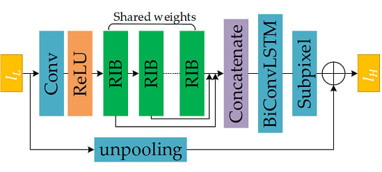
As shown in Figure 4, our BCLSR mainly consisted of the following modules: the convolution layer for learning low-level features, the recursive inference block (RIB) to extract hierarchical features, the BiConvLSTM layer to fuse the hierarchical features, and the sub-pixel layer [22] to transform feature maps into the HR image space.

We denote $I_L$ as the given LR images, and $I_H$ as the target HR images. Due to the high correlation of $I_L$ and $I_H$, we upsampled the LR to the size of HR in the global residual path $F_G$ by the nearest interpolation. In the residual body, a single convolution layer $con{v}_s$ with a kernel size of 3 × 3 extracts low-level features from the LR input for further feature inference:

$$F_0=\max (0,con{v}_s\left(I_L\right))$$

(3)

where $F_0$ is used as the input to the recursive inference blocks (details about the RIB are presented in Section 2.3). Hence, we further have the recursions by:

$$F_{\mathrm{n}}=S_{RIB}^n\left(F_0\right)$$

(4)

where $RI{B}^n$ denotes the operation of the n-fold recursive inference block and $F_{\mathrm{n}}$ (n = 1,…N) denotes the output of $\mathrm{n}$-$\mathrm{th}$ RIB. BiConvLSTM takes the concatenation of all results as an input according to the order of recursion.

$$F_{\mathrm{fuse}}=BCL\left([F_{\mathrm{n}},F_{n-1},\dots ,F_1\right])$$

(5)

Then, we concatenated the hidden states of BiConvLSTM and passed through the subpixel layer, then we added the output of the subpixel layer with the upsampled LR $F_G$ as the reconstruction.

2.3. Recursive Inference Block

Here, we introduce the details of the recursive inference block (RIB), as shown in Figure 5. Our RIB contained a feature-expanding layer, densely-connected layers, and a local feature-fusion layer. Let us denote $con{v}_e$ as the first feature-expanding layer and $con{v}_{d,i}$ as the $\mathrm{i}$-$\mathrm{th}$ layer in densely-connected layers.

(1) Feature expanding layer: We used a 1 × 1 convolution layer for feature expansion to allow more information to pass through, which is widely used for channel number expansion or reduction in ResNet [24], and then applied the non-linearity activation function (ReLUs) after the convolution layer to keep the non-linearity. We denoted the output of the feature-expanding layers as

$$F_{n,0}=\max (0,con{v}_e\left(F_{n-1}\right))$$

(6)

where $F_{n-1}$ denotes the output from the last recursion, and $F_{n,0}$ is then used as the input to the densely-connected layer for further feature extraction.

(2) Densely-connected layer: In the structure of densely-connected layers, paths are created between a layer and every preceding layer. This strengthens the flow of information through deep networks and reuses the features extracted in previous layers refraining from the learning redundant feature, and thus, alleviates the vanishing gradient problem [28]. The $\mathrm{i}$-$\mathrm{th}$ layer $con{v}_{d,i}$ in the densely-connected layers concatenates the features of all of the preceding layers as the input, which can be formulated as

$$F_{n,i}=\max (0,con{v}_{d,i}\left(\left[F_{n,0},F_{n,1},\dots ,F_{n,i-1}\right]\right))$$

(7)

where $\left[F_{n,0},F_{n,1},\dots ,F_{n,i-1}\right]$ represents the concatenation of the outputs in all of the preceding layers of the $\mathrm{i}$-$\mathrm{th}$ layer in the $\mathrm{n}$-$\mathrm{fold}$ RIB.

(3) Feature fusion layer: Since the output of the $\mathrm{n}$-$\mathrm{th}$ fold RIB will be the input of the (n + 1)-th fold RIB, it is essential to introduce a convolutional layer $con{v}_f$ to keep the same feature channel number and fuse the local feature maps. We assumed that these are D densely-connected layers, each consisting of G feature maps, and the channel number of the feature expanding layer is E. Hence, the concatenation of all preceding outputs will have D × G + E features. To further enhance the capacity of the RIB and improve the flow of information, we introduced a local residual path between the input and output of the RIB, hence the final output of the n-th fold RIB can be obtained by:

$$F_n=F_{n-1}+\max \left(0,con{v}_f\left(\left[F_{n,0},F_{n,1},\dots ,F_{n,d}\right]\right)\right)$$

(8)

We set 1 × 1 as the kernel size of the feature fusion layer to selectively fuse the features from the previous densely-connected layers in the current stages. After the local residual learning, each recursion applies the same inference block with the shared weights, and hence Equation (6) can also be formulated as:

$$F_n=S_{RIB}^n\left(F_0\right)=S_{RIB}\left(S_{RIB}\left(\dots S_{RIB}\left(F_0\right)\right)\right)$$

(9)

2.4. BiConvLSTM

To fuse the hierarchical features extracted from the recursive inference block, a bidirectional convolutional LSTM cell was used to access the long-range context, as shown in Figure 6. The input, which is the concatenation of all recursive inference block outputs according to the sequence, is denoted as $\left[F_n,F_{n-1},\dots ,F_1\right]$. ConvLSTM [49] and BiConvLSTM [50] are usually used to learn global, long-term spatiotemporal features of videos. In our approach, we considered the recursions of RIB as a temporal sequence in the order of the recursion.

(1) BiConvLSTM layer: A BiConvLSTM cell essentially contains several ConvLSTM cells with two cell states, separately a forward sequence cell and a backward sequence cell, to model the series dependency from both the previous and next recursions, and can thereby access long-range dependency features in both directions of the recursion sequence. The formulation of the forward or backward ConvLSTM cell can be obtained by:

$$i_n^f=\mathsf{\sigma }\left(W_{fi}^f\ast F_n+W_{hi}^f\ast H_{n-1}^f+b_i^f\right)$$

(10)

$$f_n=\mathsf{\sigma }\left(W_{ff}\ast F_n+W_{hf}\ast H_{n-1}+b_f\right)$$

(11)

$$o_n=\mathsf{\sigma }\left(W_{fo}\ast F_n+W_{ho}\ast H_{n-1}+b_o\right)$$

(12)

$$C_n=f_n\odot C_{n-1}+i_n\ast \tan \mathrm{h}\left(W_{fc}\ast F_n+W_{hc}\ast H_{n-1}+b_c\right)$$

(13)

$$H_n^f=o_n\odot \tan \mathrm{h}\left(C_n\right)$$

(14)

where “$\ast$” denotes the convolution operation; “$\odot$” denotes the Hadamard product; and “$\mathsf{\sigma }$” denotes the sigmoid function. $W_{f\ast }^f$ and $W_{h\ast }^f$ represent the convolution kernels for the input stage and hidden stage in the forward ConvLSTM cell, respectively.

(2) Multi-BiConvLSTM layer: We denoted the $\mathrm{i}$-$\mathrm{th}$ ConvLSTM layer forward sequence hidden and cell states as ($h_f^i$,$c_f^i$) and the backward sequence hidden states and cell states as ($h_b^i$,$c_b^i$). We concatenated the corresponding hidden forward and backward hidden states in the first layer and passed them through a 3 × 3 convolutional layer to obtain the hidden representations as the input of the second BiConvLSTM layer. Then, we concatenated the hidden representations of the second BiConvLSTM layer for the input of the upscaling layer.

2.5. Global Residual Path

Since super-resolution is an image-to-image translation task where the input LR image is highly correlated with the target HR image, learning the residuals between LR and HR avoids learning a complicated transformation from a complete image to another. Most models [16,17,18] based on a global residual path use a single convolution layer with a kernel size bigger than 5 × 5 to extract the low-level features. Because the residuals in most regions are close to zero, the model complexity and learning difficulty are greatly reduced. By adopting the global residual learning, the main body of our network is only required to learn a residual map to restore the missing high-frequency details. We argue that the convolutional layer is actually not necessary for low-level feature extraction, hence, we directly unpooled the input LR images to the size of HR images to construct the global residual path. The upsampling methods should keep the main structure and low-frequency information of LR without too much computation cost. In our experiments, we used the nearest interpolation method to upsample LR in the global path, and we found this upsampling strategy slightly improved the accuracy and simultaneously reduced the parameters and computations.

3. Results

In this section, we evaluated the methods introduced in Section 2 on multispectral remote sensing images. Section 3.1 features detailed descriptions of the evaluation process and our training setup. We undertook several experiments to understand the properties of our model, and the effect of increasing the number of recursions is investigated in Section 3.2 and Section 3.3. Finally, we compared our method with several state-of-the-art methods in Section 3.4. Our codes are available [51].

3.1. Implementation Details

Our models were optimized with Adam [52] by setting β₁ = 0.9 and β₂ = 0.999, and the initial learning rate was set to 1 × 10⁻³ and decreased by a factor of two every 10 epochs. We implemented our proposed method via the Pytorch framework and trained them using NVIDIA 1080Ti GPUs, and the batch size was set to 16. For multispectral and panchromatic satellite images, we divided each channel as the input with a different model and for nature remote sensing images; we used three-channel images for the model training. Hence, for different image types, we slightly modified the channel of the reconstruction layer as three or one.

3.2. Study of Recursive Inference Block

To study the effect of increasing recursion depth, we trained five models with different numbers of recursions: 2, 4, 8, 16, and 32. To clearly show how recursions affected the performance, the five models used the same inference block structure as described in Section 2 and set the growth-rate as 16 in the RIB, hence each model had the same parameters.

Table 1. Model comparisons at different recursion numbers in terms of PSNR and SSIM on the COWC datasets for the scale factor ×2. The deeper model with more recursions achieved a better performance because of the larger conceptive fields and more nonlinearities, while the processing time per tile also increased.

Recursion	PSNR (dB)	SSIM	Processing Time (s)
2	35.9383	0.9621	0.0193
4	36.2135	0.9632	0.0322
8	36.5686	0.9641	0.0469
16	36.8825	0.9650	0.0721
32	37.0531	0.9652	0.1398

shows the average PSNR and SSIM results for each model on the COWC testing sets at a scale factor ×2. It was found that by implying more recursions, both the PSNR and SSIM performances increased, while the processing time per 256 × 256 tiles also increased. For the deeper model with larger receptive fields, vastly contextual information could be utilized to infer the lost high-frequency of HR images, and by using the ReLU activation layer after each convolutional layer, the deeper model with more nonlinearities could model more complex mapping functions to further improve performance. Due to recursive learning, our deeper model with more recursions could increase performance, but without additional parameters, and this strategy kept our model more compact when the recursions were increased.

3.3. Study of BiConvLSTM

In this subsection, to investigate the effects of the BiConvLSTM layer, we tested two other different fusion strategies to fuse all of the hierarchical features, specifically by adding and concatenating all of the recursions before the upsampling layer. We also tested our recursive model without a fusion strategy and put the features from the last recursion to the upsampling layer to reconstruct the HR images. We also tested our recursive model without a fusion strategy and put the features from the last recursion to the upsampling layer to reconstruct the HR images.

For a fair comparison, all models used the same four-fold RIB that differed only in the fusion blocks.

Table 2. Comparison of the average results on the COWC testing sets in terms of PSNR and SSIM for the scale factor ×2 by using different strategies to fuse the hierarchical features. Selectively extracting information from low-level features further improved the model performance.

Fusion Strategy	PSNR (dB)	SSIM
Without fusion	35.9637	0.9571
Add	35.9522	0.9565
Concate	36.0312	0.9573
BiConvLSTM	36.2135	0.9632

shows the mean PSNR and SSIM results on the COWC testing sets of the different strategies at a scale factor ×2. As expected, the concatenation strategy obtained better performance than the model without fusing the hierarchical feature, which indicates that the low-level features provide essential information in the SR task. The strategy of adding all recursions was even worse than that without fusion, indicating that using low-level features without any selection or weights can actually impede the flow of information. Additionally, our BiConvLSTM strategy reduced redundant and extracted complementary information from the low-level features by exploiting the dependency and correlations of different level features, which further promoted the performance.

3.4. Result Comparison

In this subsection, we evaluate the performance of our proposed BCLSR on the test set with different upsampling factors, and compared it with some other methods including bicubic interpolation, the classic CNN-based SRCNN [15], VDSR [16], EDSR [17], WDSR [18], and RDN [29]. For a fair and convincing comparison, we slightly adjusted these methods and trained these networks under our experimental dataset to obtain their best performance. For SRCNN [15], we used a 9-5-5 model for comparison. For VDSR [16], EDSR [17], and WDSR [18], we used their public code and set four residual blocks to have the same model depth. For RDN [29], we set their growth-rate as 16. Considered with both speed and accuracy, our model used the 16-fold recursive inference block for comparison and set the growth rate as 16.

Table 3. Average PSNR/SSIM results at scales ×2, ×3, and ×4 on our GF-2 datasets and the COWC datasets. The red color indicates the best performance.

Dataset	Scale	Bicubic	SRCNN [15]	VDSR [16]	EDSR [17]	WDSR [18]	RDN [29]	Ours
multi	×2	22.3621/0.7298	24.6636/0.8524	25.7425/0.8541	26.2432/0.8576	26.9592/0.8654	27.0114/0.8661	28.0520/0.8794
	×3	21.9478/0.7148	24.1481/0.8361	24.8528/0.8436	25.6459/0.8493	26.3841/0.8567	26.3419/0.8589	27.1440/0.8633
	×4	21.6421/0.7194	23.7349/0.8219	24.1731/0.8368	24.5481/0.8419	25.1729/0.8485	25.1691/0.8490	25.9240/0.8538
pan	×2	23.4583/0.7605	26.8830/0.8523	27.8478/0.8624	27.9691/0.8731	28.5572/0.8874	28.5426/0.8852	29.4159/0.8925
	×2	22.9761/0.7384	26.2414/0.8142	26.8993/0.8632	27.2823/0.8659	27.9147/0.8745	28.0278/0.8751	28.9123/0.8798
	×4	21.7494/0.7129	25.6932/0.7942	25.7667/0.8223	25.8215/0.8434	26.5937/0.8512	26.6042/0.8551	26.9434/0.8672
COWC	×2	30.5916/0.9154	33.9821/0.9521	35.2361/0.9598	35.6907/0.9623	35.9886/0.9625	35.9746/0.9636	36.8825/0.9650
	×3	29.1484/0.8241	31.4164/0.8542	31.9672/0.8764	32.4897/0.8954	32.9545/0.9078	33.0746/0.9103	33.9843/0.9286
	×4	28.8461/0.7987	30.1873/0.8073	31.0381/0.8531	31.5901/0.8862	31.6792/0.8891	31.7273/0.8934	32.5528/0.8952

presents the ultimate mean PSNR and SSIM over the test images of these methods for ×2, ×3, and ×4 upsampling factors. In terms of PSNR, our method achieved an improvement of about 0.9 dB over state-of-the-art results on different datasets, but with fewer parameters. As the spatial resolution of GF-2 images are 4 m and 1 m, too much high-frequency information is lost, which leads to the average PSNR and SSIM of the GF-2 dataset being commonly lower than that of the COWC dataset.

Figure 7 shows the comparisons of the SR results of these methods on the COWC test set, where our method could well reconstruct the contours of cars. Figure 8 shows the multispectral satellite images with blue, green, and red channels, and Figure 9 shows the panchromatic channel images. Our methods reconstructed a sharper and clear roof with fewer artifacts, and models like RDN [29], which have too many parameters, were more likely to over-fit, so their performance could be degraded with over-training.

We also tested these models with original images to generate SR results. There are many non-reference quality metrics [53,54,55] to quantify these real-data results. Our experimental datasets contain natural images, multispectral images, and panchromatic images, hence we employed BRISQUE [55] metric to quantify the qualities of different types of reconstruction images without references. We used these models trained under our experimental dataset at a scale factor ×3 and took the original spatial resolution images as inputs to yield SR results.

Table 4. Average BRISQUE results at scales ×2, ×3, and ×4 on our GF-2 datasets and the COWC datasets. The red color indicates the best performance.

Dataset	Scale	Bicubic	SRCNN [15]	VDSR [16]	EDSR [17]	WDSR [18]	RDN [29]	Ours
multi	×2	49.0127	45.9521	42.8894	40.0320	38.5421	37.2690	35.5900
	×3	53.1440	50.1416	49.7040	48.9662	45.7588	44.8927	43.2459
	×4	61.3699	58.9284	55.0017	53.2863	51.9466	50.6996	49.3648
pan	×2	46.7117	42.2646	40.4815	39.7721	34.9061	35.9469	32.6524
	×3	55.6381	52.46823	49.6719	47.2730	44.8361	43.3989	41.6488
	×4	59.3537	56.7083	53.6317	52.3405	49.1415	48.4533	47.1435
COWC	×2	38.2804	35.7388	34.8030	32.6975	30.9478	29.4001	28.1540
	×3	46.5723	45.5027	41.3250	40.9971	35.7353	36.1159	34.1814
	×4	52.1886	48.4841	45.7582	43.9544	41.6560	40.3677	38.3023

presents the ultimate mean BRISQUE over the test images of these methods for ×2, ×3, and ×4 upsampling factors.

Figure 10, Figure 11 and Figure 12 show the results at scales ×3 on the COWC test set, GF-2 multispectral images, and the panchromatic images at the original spatial resolution, respectively.

3.5. Cross-Validation Experiments

In this subsection, for further assessing how results of a statistical analysis will generalize to an independent dataset, we compared our method with several state-of-art methods as described in Section 3.4. For our cross-validation experiments, following Carranza-García et al. [56], we randomly split COWC datasets into five equal-sized folds where each one fold is reserved for testing and the other four are used for training. We repeatedly trained each model five times at a scale factor ×4, and hence obtained five test accuracies for each model. We then calculated the mean and standard deviation of all test accuracies.

Figure 13 shows the mean and standard deviation of PSNR on COWC datasets. Our method outperformed the RDN [29] by about 0.3 dB, and the standard deviation is ±0.0674 dB, which demonstrate the effectiveness of our method. Furthermore, compared with methods based on deep learning, the standard deviation of bicubic interpolation method 0.023 dB is smaller than other data-driven methods. Nonetheless, the standard deviations of other methods are all below 0.08 dB and the accuracies are much higher than the interpolation method.

4. Discussion

(1) Difference to SRCNN and VDSR: First, SRCNN [15] and VDSR [16] needed to upsample the original LR image to the desired size using Bicubic interpolation. This procedure results in feature extraction and reconstruction in the HR space, while BCLSR extracts hierarchical features from the original LR image, reducing computational complexity significantly and improving the performance. Secondly, SRCNN [15] and VDSR [16] used L2 loss function while we utilize the L1 loss function, which has been demonstrated to be more powerful for performance and convergence.

(2) Difference to EDSR and WDSR: First, both EDSR [17] and WDSR [18] applied global residual learning and local residual learning, but the global residual path of EDSR [17] and WDSR [18] are the addition of low-level features and high-level features, which is computationally expensive. While in BCLSR, as shown in Section 2.5, we directly introduced the nearest interpolation path to upsample LR to the size of HR, forming the global residual path, which can accelerate the convergence. Secondly, there is no dense connections among EDSR [17] and WDSR [18]. BCLSR adopts the densely-connected structure to reuse low-level features to provide richer information for reconstructing high-quality details.

(3) Difference to RDN: RDN [29] also built upon the dense connection and constructed the basic local dense block, while BCLSR utilized the recursive learning strategy and repeatedly applied the same inference block, which can reduce the storage demand and keep a concise model while increasing its depth. Secondly, RDN [29] concatenated all feature-maps produced by residual dense blocks and then used a composite function of 1 × 1 and 3 × 3 convolution layer to fuse this concatenation. However, as demonstrated in Section 3.3, this fusion strategy cannot fully extract global features. BCLSR applied the BiConvLSTM layer to selectively extract complementary information from different level features and avoids passing through redundant feature to the reconstruction layer.

(4) Parameters-to-PSNR comparison: To further compare the processing time and number of parameters of different methods, in Figure 14, we illustrate the parameters-to-PSNR relationship on the COWC testing sets at a scale factor ×2 of our model with recursions 4,8,16 (denoted as BCLSR_R4, BCLSR_R8, BCLSR_R16), SRCNN [15], VDSR [16], EDSR [17], WDSR [18], and RDN [29]. The proposed BCLSR benefits from inherent parameter sharing and therefore obtains higher parameter efficiency compared to other methods, and the local dense connection reuses the local low-level feature, strengthening the information flow with each recursion. Besides that, due to the variant scale of objects in remote sensing images, the BiConvLSTM layer extracts complementary information from different level recursions and provides additional information to reconstruct the HR images. As demonstrated in Figure 14, while the BiConvLSTM layer is a relatively time-consuming process compared with RDN [29], our method outperforms RDN with fewer parameters and our method represents a reasonable trade-off between model size and SR performance with modest inference time.

(5) Failed cases: As the spatial resolution of GF-2 images are only 4 m and 1 m, too much high-frequency information is lost especially in the area full of buildings. As shown in Figure 15, the reconstruction of the white road is much better than the dense buildings at a scale of ×4. It is quite a common phenomenon for large scale reconstruction that too much loss of information usually makes SR methods fail to recover the fine details and the reconstruction result over-smooth.

5. Conclusions

In this paper, we proposed a novel network BCLSR for remote sensing image SR tasks that employed a recursive inference block and a BiConvLSTM layer to separately extract and fuse the hierarchical features. Our model mainly benefits from three aspects: (1) since the receptive field is widened with each recursion, more contextual information can be utilized for reconstruction without additional parameters; (2) by reusing the local low-level feature, information flow can be strengthened from LR to HR through the deep model, alleviating exploded or vanished gradients; (3) the BiConvLSTM layer selectively extracts complementary information from all recursions and avoids passing through a redundant feature to the reconstruction layer. Compared with other fusion strategies, our experiments also demonstrated that by using the BiConvLSTM layer to exploit the dependency and correlations of different level features, this could promote reconstruction performance. The experiment results on multispectral satellite images, panchromatic satellite images, and nature high-resolution remote sensing images demonstrated that the proposed method BCLSR outperformed state-of-the-art methods with fewer parameters. Our future work will focus on: (1) in remote sensing areas, some computer version tasks such as objection detection, due to the small size of objection in remote sensing images, the SR task can improve the ability of objection detection. Hence, we will combine our SR method with a real-time objection detection task on remote sensing images to further evaluate the effectiveness of our methods by reducing the processing time; and (2) SR with guidance is attracting more attention, and the auxiliary information from guidance can improve the reconstruction quality. In the remote sensing area, the similar idea pansharpening is a fundamental and significant task in the field of remote sensing imagery processing, in which high-resolution spatial details from panchromatic images are employed to enhance the spatial resolution of MS images. Hence, another direction of our future work will be to try to incorporate the panchromatic bands to improve the resolution of the multispectral bands’ images by building a deep pansharpening model.

References

- Merino, M.T.; Nunez, J. Super-resolution of remotely sensed images with variable-pixel linear reconstruction. IEEE Trans. Geosci. Remote Sens. 2007, 45, 1446–1457. [Google Scholar] [CrossRef]
- Yang, D.; Li, Z.; Xia, Y.; Chen, Z. Remote sensing image super-resolution: Challenges and approaches. In Proceedings of the 2015 IEEE International Conference on Digital Signal Processing (DSP), Singapore, 21–24 July 2015; pp. 196–200. [Google Scholar]
- Harris, J.L. Diffraction and resolving power. JOSA 1964, 54, 931–936. [Google Scholar] [CrossRef]
- Goodman, J.W. Introduction to Fourier optics; McGraw-Hill: San Francisco, CA, USA, 2005. [Google Scholar]
- Tsai, R. Multiframe image restoration and registration. Adv. Comput. Vis. Image Process. 1984, 1, 317–339. [Google Scholar]
- Yang, J.; Wright, J.; Huang, T.S.; Ma, Y. Image super-resolution via sparse representation. IEEE Trans. Image Process. 2010, 19, 2861–2873. [Google Scholar] [CrossRef] [PubMed]
- Zhang, Y.; Wu, W.; Dai, Y.; Yang, X.; Yan, B.; Lu, W. Remote sensing images super-resolution based on sparse dictionaries and residual dictionaries. In Proceedings of the 2013 IEEE 11th International Conference on Dependable, Autonomic and Secure Computing, Chengdu, China, 21–22 December 2013; pp. 318–323. [Google Scholar]
- Zhang, H.; Huang, B. Scale conversion of multi sensor remote sensing image using single frame super resolution technology. In Proceedings of the 2011 19th International Conference on Geoinformatics, Shanghai, China, 24–26 June 2011; pp. 1–5. [Google Scholar]
- Czaja, W.; Murphy, J.M.; Weinberg, D. Superresolution of Noisy Remotely Sensed Images Through Directional Representations. IEEE Geosci. Remote Sens. Lett. 2018, 1–5. [Google Scholar] [CrossRef]
- Ahi, K. Mathematical modeling of THz point spread function and simulation of THz imaging systems. IEEE Trans. Terahertz Sci. Technol. 2017, 7, 747–754. [Google Scholar] [CrossRef]
- Ahi, K. A method and system for enhancing the resolution of terahertz imaging. Measurement 2019, 138, 614–619. [Google Scholar] [CrossRef]
- Chernomyrdin, N.V.; Frolov, M.E.; Lebedev, S.P.; Reshetov, I.V.; Spektor, I.E.; Tolstoguzov, V.L.; Karasik, V.E.; Khorokhorov, A.M.; Koshelev, K.I.; Schadko, A.O. Wide-aperture aspherical lens for high-resolution terahertz imaging. Rev. Sci. Instrum. 2017, 88, 014703. [Google Scholar] [CrossRef]
- Chernomyrdin, N.V.; Schadko, A.O.; Lebedev, S.P.; Tolstoguzov, V.L.; Kurlov, V.N.; Reshetov, I.V.; Spektor, I.E.; Skorobogatiy, M.; Yurchenko, S.O.; Zaytsev, K.I. Solid immersion terahertz imaging with sub-wavelength resolution. Appl. Phys. Lett. 2017, 110, 221109. [Google Scholar] [CrossRef]
- Nguyen Pham, H.H.; Hisatake, S.; Minin, O.V.; Nagatsuma, T.; Minin, I.V. Enhancement of spatial resolution of terahertz imaging systems based on terajet generation by dielectric cube. Apl Photonics 2017, 2, 056106. [Google Scholar] [CrossRef] [Green Version]
- Dong, C.; Loy, C.C.; He, K.; Tang, X. Learning a deep convolutional network for image super-resolution. In Proceedings of the European conference on computer vision, Zurich, Switzerland, 6–12 September 2014; pp. 184–199. [Google Scholar]
- Kim, J.; Kwon Lee, J.; Mu Lee, K. Accurate image super-resolution using very deep convolutional networks. In Proceedings of the IEEE conference on computer vision and pattern recognition, Las Vegas, NV, USA, 26 June–1 July 2016; pp. 1646–1654. [Google Scholar]
- Lim, B.; Son, S.; Kim, H.; Nah, S.; Mu Lee, K. Enhanced deep residual networks for single image super-resolution. In Proceedings of the IEEE Conference on Computer Vision and Pattern Recognition Workshops, Honolulu, HI, USA, 21–26 July 2017; pp. 136–144. [Google Scholar]
- Yu, J.; Fan, Y.; Yang, J.; Xu, N.; Wang, Z.; Wang, X.; Huang, T. Wide activation for efficient and accurate image super-resolution. arXiv 2018, arXiv:1808.08718. Available online: https://arxiv.org/abs/1808.08718 (accessed on 21 December 2018).
- Dong, C.; Loy, C.C.; Tang, X. Accelerating the super-resolution convolutional neural network. In Proceedings of the European conference on computer vision, Amsterdam, The Netherlands, 8–16 October 2016; pp. 391–407. [Google Scholar]
- Shi, W.; Caballero, J.; Huszár, F.; Totz, J.; Aitken, A.P.; Bishop, R.; Rueckert, D.; Wang, Z. Real-time single image and video super-resolution using an efficient sub-pixel convolutional neural network. In Proceedings of the IEEE conference on computer vision and pattern recognition, Las Vegas, NV, USA, 26 June–1 July 2016; pp. 1874–1883. [Google Scholar]
- Ahn, N.; Kang, B.; Sohn, K.-A. Image super-resolution via progressive cascading residual network. In Proceedings of the IEEE Conference on Computer Vision and Pattern Recognition Workshops, Salt Lake City, UT, USA, 18–22 June 2018; pp. 791–799. [Google Scholar]
- Kim, J.; Kwon Lee, J.; Mu Lee, K. Deeply-recursive convolutional network for image super-resolution. In Proceedings of the IEEE conference on computer vision and pattern recognition, Las Vegas, NV, USA, 26 June–1 July 2016; pp. 1637–1645. [Google Scholar]
- Tai, Y.; Yang, J.; Liu, X. Image super-resolution via deep recursive residual network. In Proceedings of the IEEE conference on computer vision and pattern recognition, Honolulu, HI, USA, 21–26 July 2017; pp. 3147–3155. [Google Scholar]
- He, K.; Zhang, X.; Ren, S.; Sun, J. Deep residual learning for image recognition. In Proceedings of the IEEE conference on computer vision and pattern recognition, Las Vegas, NV, USA, 26 June–1 July 2016; pp. 770–778. [Google Scholar]
- Ledig, C.; Theis, L.; Huszár, F.; Caballero, J.; Cunningham, A.; Acosta, A.; Aitken, A.; Tejani, A.; Totz, J.; Wang, Z. Photo-realistic single image super-resolution using a generative adversarial network. In Proceedings of the IEEE conference on computer vision and pattern recognition, Honolulu, HI, USA, 21–26 July 2017; pp. 4681–4690. [Google Scholar]
- Ran, Q.; Xu, X.; Zhao, S.; Li, W.; Du, Q. Remote sensing images super-resolution with deep convolution networks. Multimed. Tools Appl. 2019, 1–17. [Google Scholar] [CrossRef]
- Huang, G.; Liu, Z.; Van Der Maaten, L.; Weinberger, K.Q. Densely connected convolutional networks. In Proceedings of the IEEE conference on computer vision and pattern recognition, Honolulu, HI, USA, 21–26 July 2017; pp. 4700–4708. [Google Scholar]
- Tong, T.; Li, G.; Liu, X.; Gao, Q. Image super-resolution using dense skip connections. In Proceedings of the IEEE International Conference on Computer Vision, Venezia, Italy, 22–29 October 2017; pp. 4799–4807. [Google Scholar]
- Zhang, Y.; Tian, Y.; Kong, Y.; Zhong, B.; Fu, Y. Residual dense network for image super-resolution. In Proceedings of the IEEE Conference on Computer Vision and Pattern Recognition, Salt Lake City, UT, USA, 18–23 June 2018; pp. 2472–2481. [Google Scholar]
- Tai, Y.; Yang, J.; Liu, X.; Xu, C. Memnet: A persistent memory network for image restoration. In Proceedings of the IEEE International Conference on Computer Vision, Venezia, Italy, 22–29 October 2017; pp. 4539–4547. [Google Scholar]
- Ahn, N.; Kang, B.; Sohn, K.-A. Fast, accurate, and lightweight super-resolution with cascading residual network. In Proceedings of the European Conference on Computer Vision (ECCV), Munich, Germany, 8–14 September 2018; pp. 252–268. [Google Scholar]
- Wang, X.; Yu, K.; Wu, S.; Gu, J.; Liu, Y.; Dong, C.; Qiao, Y.; Change Loy, C. Esrgan: Enhanced super-resolution generative adversarial networks. In Proceedings of the European Conference on Computer Vision (ECCV), Munich, Germany, 8–14 September 2018. [Google Scholar]
- Haris, M.; Shakhnarovich, G.; Ukita, N. Deep back-projection networks for super-resolution. In Proceedings of the IEEE Conference on Computer Vision and Pattern Recognition, Salt Lake City, UT, USA, 18–23 June 2018; pp. 1664–1673. [Google Scholar]
- Sajjadi, M.S.; Vemulapalli, R.; Brown, M. Frame-recurrent video super-resolution. In Proceedings of the IEEE Conference on Computer Vision and Pattern Recognition, Salt Lake City, UT, USA, 18–23 June 2018; pp. 6626–6634. [Google Scholar]
- Huang, Y.; Wang, W.; Wang, L. Bidirectional recurrent convolutional networks for multi-frame super-resolution. In Proceedings of the Advances in Neural Information Processing Systems, Montréal, QC, Canada, 7–12 December 2015; pp. 235–243. [Google Scholar]
- Huang, Y.; Wang, W.; Wang, L. Video super-resolution via bidirectional recurrent convolutional networks. IEEE Trans. on pattern Anal. Mach. Intell. 2017, 40, 1015–1028. [Google Scholar] [CrossRef] [PubMed]
- Guo, J.; Chao, H. Building an end-to-end spatial-temporal convolutional network for video super-resolution. In Proceedings of the Thirty-First AAAI Conference on Artificial Intelligence, San Francisco, CA, USA, 4–10 February 2017. [Google Scholar]
- Liao, Q.; Poggio, T. Bridging the gaps between residual learning, recurrent neural networks and visual cortex. arXiv 2016, arXiv:1604.03640. Available online: https://arxiv.org/abs/1604.03640 (accessed on 13 April 2016).
- Chen, Y.; Jin, X.; Kang, B.; Feng, J.; Yan, S. Sharing Residual Units Through Collective Tensor Factorization To Improve Deep Neural Networks. In Proceedings of the Twenty-Seventh International Joint Conference on Artificial Intelligence (IJCAI-18), Stockholm, Sweden, 13–19 July 2018; pp. 635–641. [Google Scholar]
- Han, W.; Chang, S.; Liu, D.; Yu, M.; Witbrock, M.; Huang, T.S. Image super-resolution via dual-state recurrent networks. In Proceedings of the IEEE Conference on Computer Vision and Pattern Recognition, Salt Lake City, UT, USA, 18–23 June 2018; pp. 1654–1663. [Google Scholar]
- Hua, Y.; Mou, L.; Zhu, X.X. Recurrently exploring class-wise attention in a hybrid convolutional and bidirectional LSTM network for multi-label aerial image classification. ISPRS J. Photogramm. Remote Sens. 2019, 149, 188–199. [Google Scholar] [CrossRef]
- Liu, Q.; Zhou, F.; Hang, R.; Yuan, X. Bidirectional-convolutional LSTM based spectral-spatial feature learning for hyperspectral image classification. Remote Sens. 2017, 9, 1330. [Google Scholar]
- Mou, L.; Bruzzone, L.; Zhu, X.X. Learning spectral-spatial-temporal features via a recurrent convolutional neural network for change detection in multispectral imagery. IEEE Trans. Geosci. Remote Sens. 2018, 57, 924–935. [Google Scholar] [CrossRef]
- Seydgar, M.; Alizadeh Naeini, A.; Zhang, M.; Li, W.; Satari, M. 3-D Convolution-Recurrent Networks for Spectral-Spatial Classification of Hyperspectral Images. Remote Sens. 2019, 11, 883. [Google Scholar] [CrossRef]
- Mou, L.; Ghamisi, P.; Zhu, X.X. Deep recurrent neural networks for hyperspectral image classification. IEEE Trans. Geosci. Remote Sens. 2017, 55, 3639–3655. [Google Scholar] [CrossRef]
- Liebel, L.; Körner, M. Single-image super resolution for multispectral remote sensing data using convolutional neural networks. ISPRS-International Archives of the Photogrammetry. Remote Sens. Spat. Inf. Sci. 2016, 41, 883–890. [Google Scholar]
- Mundhenk, T.N.; Konjevod, G.; Sakla, W.A.; Boakye, K. A large contextual dataset for classification, detection and counting of cars with deep learning. In Proceedings of the European Conference on Computer Vision, Amsterdam, The Netherlands, 8–16 October 2016; pp. 785–800. [Google Scholar]
- Wang, Z.; Bovik, A.C.; Sheikh, H.R.; Simoncelli, E.P. Image quality assessment: From error visibility to structural similarity. IEEE Trans. Image Process. 2004, 13, 600–612. [Google Scholar] [CrossRef] [PubMed]
- Xingjian, S.; Chen, Z.; Wang, H.; Yeung, D.-Y.; Wong, W.-K.; Woo, W.-c. Convolutional LSTM network: A machine learning approach for precipitation nowcasting. In Proceedings of the Advances in Neural Information Processing Systems, Montréal, QC, Canada, 7–12 December 2015; pp. 802–810. [Google Scholar]
- Hanson, A.; PNVR, K.; Krishnagopal, S.; Davis, L. Bidirectional Convolutional LSTM for the Detection of Violence in Videos. In Proceedings of the European Conference on Computer Vision (ECCV), Munich, Germany, 8–14 September 2018. [Google Scholar]
- BCLSR. Available online: https://github.com/ChangYunPeng/BCLSR.git (accessed on 25 June 2019).
- Kingma, D.P.; Ba, J. Adam: A method for stochastic optimization. arXiv 2014, arXiv:1412.6980. [Google Scholar]
- Yang, J.; Zhao, Y.; Yi, C.; Chan, J.C.-W. No-reference hyperspectral image quality assessment via quality-sensitive features learning. Remote Sens. 2017, 9, 305. [Google Scholar] [CrossRef]
- Mittal, A.; Soundararajan, R.; Bovik, A.C. Making a “completely blind” image quality analyzer. IEEE Signal Process. Lett. 2012, 20, 209–212. [Google Scholar] [CrossRef]
- Mittal, A.; Moorthy, A.K.; Bovik, A.C. No-reference image quality assessment in the spatial domain. IEEE Trans. Image Process. 2012, 21, 4695–4708. [Google Scholar] [CrossRef] [PubMed]
- Carranza-García, M.; García-Gutiérrez, J.; Riquelme, J.C. A Framework for Evaluating Land Use and Land Cover Classification Using Convolutional Neural Networks. Remote Sens. 2019, 11, 274. [Google Scholar] [CrossRef]
Figure 1.
Simplified structures of (a) VDSR and (b) SRDenseNet. The first strategy, (a) VDSR, uses a deeper CNN model to enlarge the receptive fields and improve the representation power. The second strategy, (b) SRDenseNet, reuses the features from shallow layers. Due to the different scale of objects in images, hierarchical features from a very deep network would provide more additional information to reconstruct the HR images.
Figure 2.
(a) skip connection: Both the global residual connection that links the input data and the output layer and the local residual connection from ResNet [24] alleviate the learning difficulty. (b) dense connection structures link all layers in the network and concatenate all of the preceding layers’ feature maps to alleviate vanishing gradients and reuse the features from shallow layers. (c) The green box refers to the recursive convolutional layer. Recursive neural networks repeatedly apply the same convolutional layers to control the parameters while achieving a large receptive field.
Figure 3.
Main contributions of our networks, consisting of two modules: a novel recursive inference block based on the dense connection with shared weights; a BiConvLSTM layer to fuse the concatenation of all recursive inference block outputs to extract complementary information. The green line denotes the recursive learning path by recursively implying the same block and the red line denotes the local residual learning path.
Figure 4.
The architecture of our proposed model. The green box refers to the recursive inference block, among which the convolutional layers share the same weights. ⊕ is the element-wise addition.
Figure 5.
The structure of our recursive inference block. The red line denotes the local residual learning path. denotes the output from the last recursion, and denotes the output of the current recursion.
Figure 6.
The structure of our BiConvLSTM layers. We concatenated all previous recursions [] in the order of the sequence as a temporal sequence. and denote the middle stage of the first hidden layer and the second layer, respectively, extracted from the forward and the backward ConvLSTM layer hidden states and .
Figure 7.
Qualitative comparisons of our model with other methods at the scale of ×3 on the COWC test sets.
Figure 8.
Qualitative comparisons of our model with other methods at the scale of ×3 on the GF-2 multispectral channels test set displayed with red, green, and blue channels.
Figure 9.
Qualitative comparisons of our model with other methods at the scale of ×3 on the GF-2 panchromatic channels test set.
Figure 10.
Qualitative comparisons of our model with other methods at the scale of ×3 on the COWC test sets at the original scale.
Figure 11.
Qualitative comparisons of our model with other methods at the scale of ×3 on the GF-2 multispectral channels test set at the original scale displayed with red, green, and blue channels.
Figure 12.
Qualitative comparisons of our model with other methods at the scale of ×3 on the GF-2 panchromatic channels test set at the original scale.
Figure 13.
The mean and standard deviation of PSNR on COWC datasets at the scale factor ×4.
Figure 14.
Comparison of the PSNR and the model size of SR methods on the COWC datasets for the scale factor ×2. The color of the point that corresponds to the bar on the right indicates the processing times with a 256 × 256 output image size on GPUs.
Figure 15.
The comparison of smooth reconstruction results and ground-truth.