Quantifying the Evapotranspiration Rate and Its Cooling Effects of Urban Hedges Based on Three-Temperature Model and Infrared Remote Sensing


Lab of Environmental and Energy Information Engineering, School of Environment and Energy, Peking University Shenzhen Graduate School, Shenzhen 518055, China
*
Author to whom correspondence should be addressed.
Remote Sens. 2019, 11(2), 202; https://doi.org/10.3390/rs11020202
Submission received: 19 December 2018
/
Revised: 14 January 2019
/
Accepted: 18 January 2019
/
Published: 21 January 2019
(This article belongs to the Special Issue Remote Sensing of the Terrestrial Hydrologic Cycle)
Abstract
:The evapotranspiration (ET) of urban hedges has been assumed to be an important component of the urban water budget and energy balance for years. However, because it is difficult to quantify the ET rate of urban hedges through conventional evapotranspiration methods, the ET rate, characteristics, and the cooling effects of urban hedges remain unclear. This study aims to measure the ET rate and quantify the cooling effects of urban hedges using the ‘three-temperature model + infrared remote sensing (3T + IR)’, a fetch-free and high-spatiotemporal-resolution method. An herb hedge and a shrub hedge were used as field experimental sites in Shenzhen, a subtropical megacity. After verification, the ‘3T + IR’ technique was proven to be a reasonable method for measuring the ET of urban hedges. The results are as follows. (1) The ET rate of urban hedges was very high. The daily average rates of the herb and shrub hedges were 0.38 mm·h−1 and 0.33 mm·h−1, respectively, on the hot summer day. (2) Urban hedges had a strong ability to reduce the air temperature. The two hedges could consume 68.44% and 60.81% of the net radiation through latent heat of ET on the summer day, while their cooling rates on air temperature were 1.29 °C min−1 m−2 and 1.13 °C min−1 m−2, respectively. (3) Hedges could also significantly cool the urban underlying surface. On the summer day, the surface temperatures of the two hedges were 19 °C lower than that of the asphalt pavement. (4) Urban hedges had markedly higher ET rates (0.19 mm·h−1 in the summer day) and cooling abilities (0.66 °C min−1 m−2 for air and 9.14 °C for underlying surface, respectively) than the lawn used for comparison. To the best of our knowledge, this is the first research to quantitatively measure the ET rate of urban hedges, and our findings provide new insight in understanding the process of ET in urban hedges. This work may also aid in understanding the ET of urban vegetation.
1. Introduction
Due to rapid urbanization, the urban thermal environment has worsened, and urban heat islands (UHI) have become a common problem in most cities around the world [1,2]. From 1961 to 2000, air temperature has increased 0.16 °C per decade in large cities in northern China [3]. Among 419 large cities around the world, the average annual daytime surface urban heat island is 1.500 ± 1.200 °C [4]. High temperatures in urban areas not only lead to more energy consumption for cooling [5] but also affect human health [6,7,8]. High temperatures and heat waves could even increase the mortality rate. In 27 European countries, over 28,000 people die every year due to exposure to extreme heat, which accounts for 0.61% of all deaths in these regions [9]. Therefore, studying how to efficiently mitigate urban thermal issues is essential for adaptive strategy under climate change and rapid urbanization.
In recent decades, various methods including changes to underlying surface materials, optimizing urban planning and designing, and the addition of vegetation have been proposed to mitigate UHI [10,11,12]. Among them, vegetation is considered one of the most effective mitigating methods [13,14]. Many studies have been conducted on the cooling effects of urban vegetation. Urban parks, urban forests, urban lawns, and green roofs can provide different degrees of cooling [15,16,17,18]. Research has shown that just a single tree could save 12–24% of cooling energy for a single-story building [19]. Sixty-three large Eucalyptus camaldulensis per hectare could reduce air temperature by 1 °C in Mexico City, while 24 large Liquidambar styraciflua trees could even reduce the air temperature by 2 °C [20]. A 147-hm2 park in Nagoya was also found to reduce the air temperature by 1.9 °C on hot days [21]. These studies showed that vegetation area, vegetation shapes and vegetation compositions could affect the microclimate [22,23,24,25], and the cooling effects of vegetation could be attributed to its shading, reflection, and evapotranspiration [26,27]. However, most of these studies focused on the cooling effects under different green space ratios and did not quantitatively estimate their ET rates and energy budget. Therefore, quantitative evaluation of the cooling effects is still a challenge.
Although ET is believed to be the most robust cooling mechanism, as it can consume large amounts of latent heat [12], observing the ET characteristics of urban vegetation is especially difficult [28,29]. As the vegetation is segmented by various artificial underlying surfaces in urban settings, it is difficult to meet the fetch requirements of traditional methods such as the Bowen ratio, eddy covariance and large aperture scintillometers [30]. ET could be estimated on a large scale by satellite remote sensing [31], but its resolution is usually too sparse on the street or neighborhoods scale. Moreover, only one image of an area could be obtained over several days. In contrast, sap flow and lysimeter data can only directly measure individual or small groups of plants [32,33]. Therefore, a fetch-free, high-spatiotemporal-resolution ET estimation method is needed to obtain accurate ET characteristics of urban vegetation.
The three-temperature model was proposed and developed to estimate ET via three temperature data points, net radiation and ground heat flux [34,35]. The surface temperature data could be obtained using thermal infrared images, and the meteorological data are easily available. It has been applied in studies on different scales, including the large catchment scale, the field scale and even on a single plant in growth chamber. It has been validated by the Penman–Monteith method, weighing lysimeter, Bowen ratio, eddy covariance, and water budget methods [36,37,38,39,40,41]. It has also been used to estimate ET of different vegetation types, such as crops, grass, and shrubs [38,42,43]. In urban area, it was used to estimate a small urban lawn’s ET and showed great consistency with the Bowen ratio method [30]. These results indicate potential applications for the proposed method to estimate ET of different urban vegetation.
Hedges are narrow bands of woody vegetation and associated organisms that separate fields and are generally composed of low dense vegetation including short woody plants, shrubs, and grasses [44,45]. It is a typical vegetation type in urban areas. During the past several years, attention has been paid to urban hedges because of their ecological functions, such as air quality purification, creation of animal habitat, and more [46,47]. However, their ET characteristics and regulation of the urban microclimate are neglected. Therefore, in this study we aim to (1) investigate the ET characteristics of two common urban hedges using the ‘3T + IR’ method in a subtropical megacity, Shenzhen, and then (2) quantify the cooling effects of the urban hedges and quantify the function of ET. This study could provide a new fetch-free and high-spatiotemporal-resolution method for estimating urban ET. It may contribute to understanding the ET of urban hedges, and then the species selection and landscape design in urban planning for urban heat island mitigation.
2. Material and Methods
2.1. Study Site
The experiment was conducted in Xili University Town, Shenzhen (approximately 22°35′40″N, 113°58′20″E, 17 m above the sea). Shenzhen is a typical costal city in southern China and has a subtropical marine climate affected strongly by the south Asian tropical monsoon. Its mean annual temperature is 22.3 °C. January is the coldest month of the year, while July is the hottest. Its mean annual precipitation is 1924.7 mm, which mainly occurs from May to September. The mean annual sunshine duration is 2060 h, and the solar radiation is as high as 5225 MJ/m2.
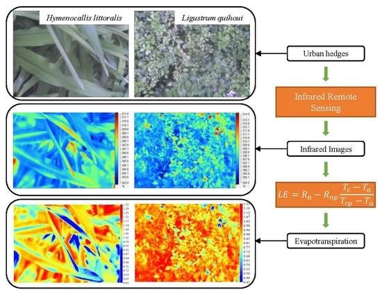
Our study site located in an open square primarily covered by urban hedges (Figure 1). The two hedges consisted of an herb, Hymenocallis littoralis (0.4 m high), and a shrub, Ligustrum quihoui (0.5 m high); both of these greening species are common in Shenzhen. The area of the H. lottoralis hedge and the L. quihoui hedge were both about 40 m2. A Zoysia matrella lawn was located nearby and used for comparison with the hedges. The lawn’s area was about 2000 m2.
2.2. Three-Temperature Model
The three-temperature model estimates vegetation ET by introducing a reference leaf with no ET [34,48].
where LE is the latent heat consumed by vegetation ET. Rn and Rnp are the net radiation on the vegetation and reference leaf, respectively (W m−2). Tc and Tp are the surface temperature of the vegetation and reference leaf (°C). The surface temperature could be obtained by thermal images, and the maximum Tc in the image is regarded as Tp [37,38]. Ta is air temperature (°C). Rn and Rnp could be estimated according to [49].
where Rs is solar radiation (W m−2). αc is the albedo of the vegetation canopy. To simplify the calculation, the empirical coefficient αc = 0.22 was used in this study [37]. ΔRl is the net long-wave radiation (W m−2), which could be estimated by [50,51]
where Rso is the clear day solar radiation (W m−2), which is assumed to equal to Rs in this study as all the experiment were conducted in clear sunny days [41]. εc the canopy emissivity, and empirical coefficient εc = 0.98 was used here [37]. σ is the Stefan–Boltzman constant (5.67 × 10⁻⁸ W m−2 K−4). εa is the atmospheric emissivity and could be estimated according to [52]
If αc, εc, and Tc are replaced by αcp, εcp and Tcp in Equations (2) and (3), then Rnp could be estimated. As we use the leaf with the highest surface temperature in the canopy as the reference leaf in this study, αc, εc are assumed to be same to αcp, εcp.
The analysis procedures were written into a software named “A system to estimate evapotranspiration by infrared remote sensing and the three-temperature model”, which can be downloaded and used freely from https://pan.baidu.com/s/19iuz5PIVjZOR96iVObYBqA.
2.3. Field Experiments
The field experiment was carried out over four typical sunny days in four seasons from 2015 to 2016, from 8:00 a.m. to 5:00 p.m. An infrared thermal imager (Fluke Ti55FT, Fluke Corp., Everett, WA, USA) was used to record the surface temperatures vertically down, at a height of 1.5 m. The measuring wavelength of the infrared thermal imager was 8–14 µm, and its resolution was 0.05 °C. The emissivity of the hedges and lawn in our study was set up to be 0.98 according to empirical value [37]. The imager could give out the emissivity-corrected temperature directly. Each thermal infrared image contains 76,800 temperature data points (320 × 240). Three images were taken of each plant at each hour. Before the measurement, the thermal camera was calibrated against a blackbody measurement.
Air temperature and other meteorological factors were recorded by a Bowen ratio system at heights of 2 m and 1.5 m. The system was installed in the middle of the lawn. All the data from the Bowen ratio system were sampled and recorded at intervals of 1 min and 10 min with a Campbell CR1000 data logger. The sensor information is shown in Table 1.
2.4. Verification Experiment
The Bowen ratio energy balance (BREB) method was used as the benchmark to verify the ‘3T + IR’ method. The verification experiment was conducted before the field experiments, on three sunny days (15 July 2014, 16 August 2014, and 13 November 2014). The ET rates of the studied area were simultaneously measured by the ‘3T + IR’ method and the BREB method. The ET rates by the BREB method could be calculated by [53]
where L is the latent heat of water vaporization (J kg−1), G is the soil heat flux (W m−2), β is the Bowen ratio, Cp is the specific heat of air at a constant pressure (J kg−1 °C−1), and ΔT and Δq are the temperature and humidity difference between the heights of 2.0 m and 1.5 m, respectively. All these parameters were obtained by the Bowen ratio system.
3. Results
3.1. Method Verification
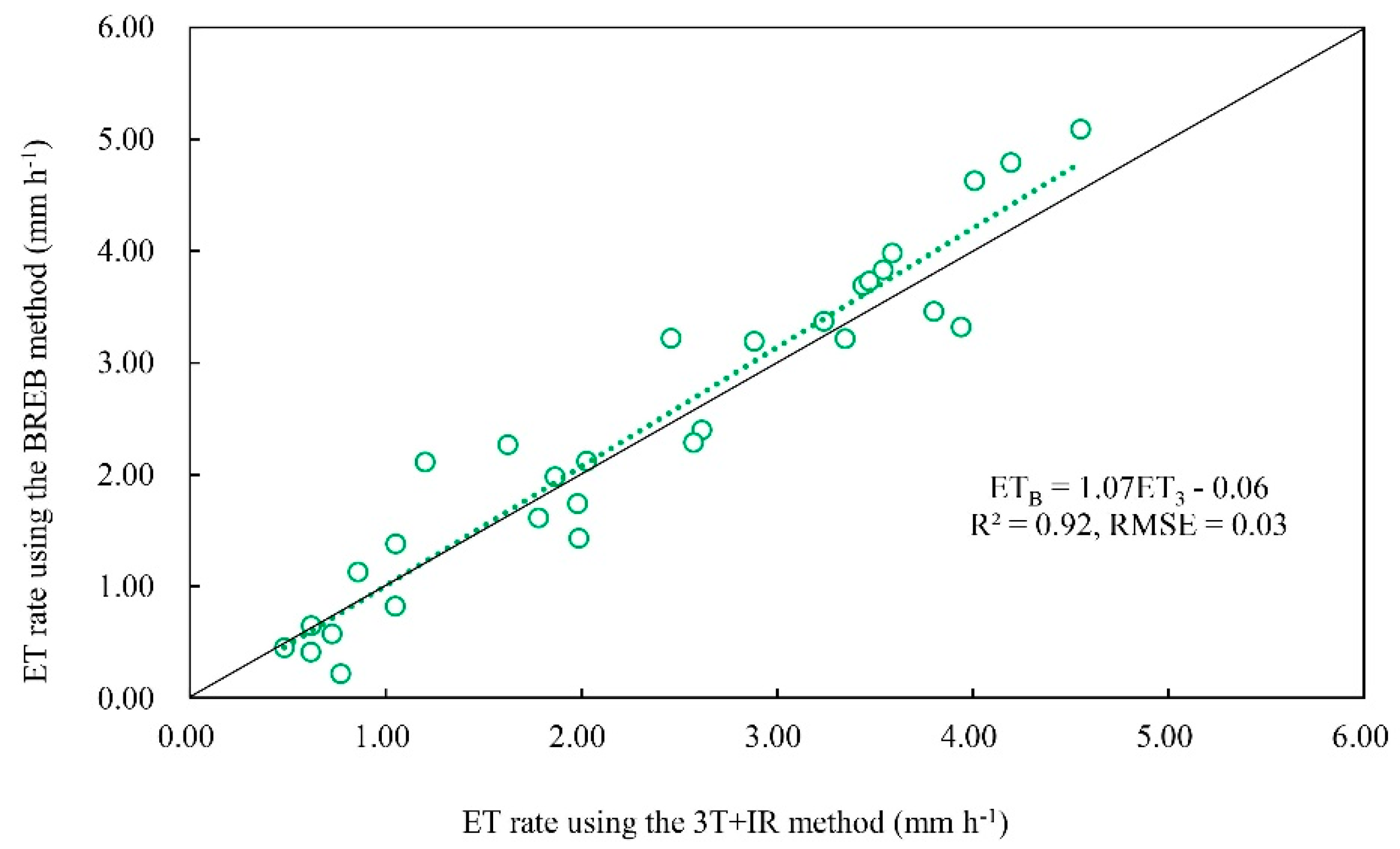
The verification experiments showed quite a coincidence between the ET rates measured by the ‘3T + IR’ method and BREB method. The correlation coefficient of the ET rates of the two methods was 0.958 (significant at the level of 0.01, by SPSS). Moreover, the linear regression demonstrated the consistency of the two methods (Figure 2). The distribution of the data was close to the 1:1 line and the regression line was ETB = 1.07ET3 – 0.06 (R2 = 0.92), which means the rates measured by ‘3T + IR’ were always close to the rates measured by BREB methods. The RMSE of the two rates was also just 0.03 mm h−1. This finding indicates that the ‘3T + IR’ method could accurately measure the ET rate of urban grass and shrubs. Therefore, we applied this method directly in the field experiments on urban hedges in this study.
3.2. Characteristics of Meteorological Conditions
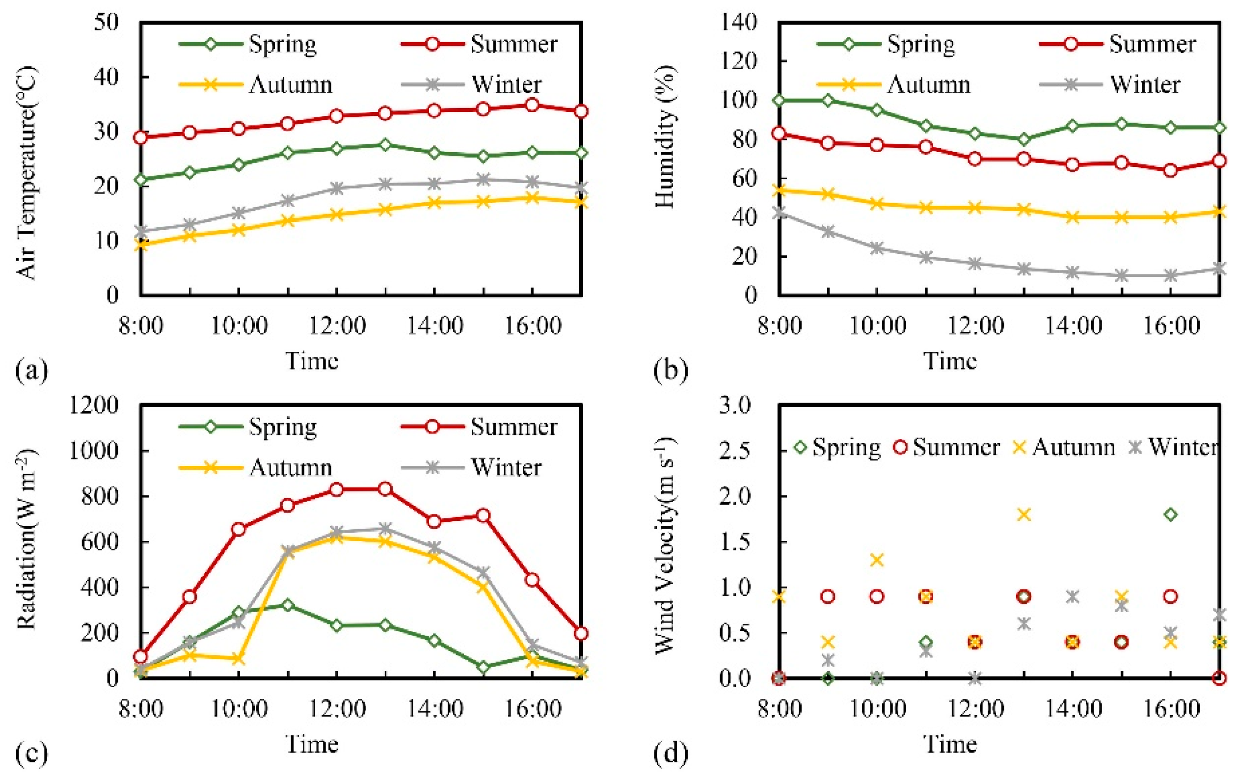
Our field experiments were conducted on a sunny day in each season from 2015 to 2016. The typical days for each season were 22 August 2015 (Summer); 18 December 2015 (Autumn); 4 February 2016 (Winter); and 19 March 2016 (Spring). The season division is according to the Shenzhen Bureau of Meteorology [54]. The daily average temperature of the summer day was as high as 32.32 °C (Figure 3). The temperatures were still high even in the autumn day (14.55 °C) and winter day (17.92 °C). The solar radiation showed an almost single-peak variation in all days. It was the strongest in the summer day, when the daily average reached 555.98 W m−2. The air was the most humid on the spring day (89%) followed by the summer day (72%). The winter day had a low relative humidity (20%). The wind velocity was not high in any of the four days. The highest was during the autumn day, when its daily average was 0.78 m s−1.
3.3. ET Characteristics of Urban Hedges
3.3.1. Surface Temperatures of the Urban Hedges
The infrared images of the hedges and the lawn were taken over four days. Subsequently, the ET rates were calculated by our software (Figure 4).
As depicted in Figure 5, the surface temperatures of the two hedges also showed single-peak variations in all four days, much like the solar radiation. For most of the time during the four days, the surface temperature of the L. quihoui hedge was higher than that of the H. littoralis hedge. The daily average surface temperature of the L. quihoui hedge was 27.43, 34.43, 20.55, and 21.94 °C in each day. At the same time, the surface temperature of the H. littoralis hedge was 26.00, 33.66, 19.77, and 20.86 °C, respectively. The surface temperatures of the hedges were slightly higher than the air temperature. The L. quihoui hedge was 2.22, 2.11, 6.00, and 4.02 °C higher than the air temperature. The smallest difference between surface and air temperature occurred during the summer day, when the solar radiation and air temperature were the highest. The surface temperature of the lawn used for comparison was much warmer than that of the two hedges. The surface temperature differences between the lawn and the H. littoralis hedge were 4.85, 9.14, 5.83, and 3.65 °C over the four days.
3.3.2. ET Rates of the Urban Hedges
The ET rates of the two hedges showed similar variation trends in the spring, autumn and winter days (Figure 6). They both increased from the morning and began to decrease after reaching peaks in the midday. The sudden drop at 11:00 a.m. during the summer day might be the result of the stomatal closure of the plants due to high surface temperatures. The ET rate was still quite high at 3:00 p.m. on the summer day. The ET of the H. littoralis hedge usually reached its maximum when the solar radiation was at its peak (Figure 3). However, the ET of the L. quihoui hedge rates reached their peaks at a different time compared to the H. littoralis hedge in the spring day. In particular, the ET rate of the L. quihoui hedge achieved another peak at 1:00 p.m. during the spring day. We also calculated the vapor pressure deficit (VPD) and found that it increased to its maximum at 1:00 p.m. during that day (data not shown).
Figure 6 also showed that the ET rates of the hedges on the summer day were obviously stronger than those of the other three days. The daily average ET rate of the H. littoralis hedge was approximately 0.38 mm h−1, while the daily average ET rate of the L. quihoui hedge was 0.33 mm h−1 (Table 2). Despite a lower level of solar radiation on the winter day, these data showed higher ET rates than on the autumn day, which may be attributed to the lowest relative humidity during this time. The ET rate was the lowest on the spring day with the lowest solar radiation and VPD. Meanwhile, we found that the ET rate of the H. littoralis hedge was higher than that of the L. quihoui hedge over the four days. The differences were 0.01, 0.05, 0.04, and 0.01 mm h−1. The ET rates of the hedges were always higher than the lawn, especially on the summer day, when the ET rate of the H. littoralis hedge was 0.20 mm h−1 higher than the lawn. The difference was the smallest on the spring day, when all the three vegetation types had low ET rates.
3.3.3. The LE/Rn of the Urban Hedges
It is usually understood that green space could cool the surrounding area through latent heat flux. To reflect the diurnal course of energy exchange, the ratio of latent to net radiation (LE/Rn) was used to illuminate the cooling effect. As shown in Figure 7, the variation of LE/Rn showed different characteristics over the four days. The LE/Rn fluctuated through the day. At 8:00 a.m. on the summer day, the LE/Rn of the two hedges could reach approximately 90%. Their LE/Rn maintained a high value during the summer day, indicating that most of the net radiation was consumed by latent heat. On the autumn and winter day, their LE/Rn had obvious changes in the morning and afternoon because of low latent heat consumption at the beginning and ending of the day.
During the summer day, the hedges could consume over 60% of the net radiation through latent heat. The ET rate was the lowest on the spring day, the LE/Rn of the hedges during that day was also the lowest. Though the LE/Rn of the L. quihoui hedge exceeded 50% at 5:00 p.m. during the spring day, its cooling effect was still negligible because the latent heat was only 0.63 W m−2. The LE/Rn of the lawn for comparison had variation trends similar to the LE/Rn of the hedges except for the summer day, which began with a small LE/Rn and was still high at 5:00 p.m.
Overall, the daily average LE/Rn of the H. littoralis hedge was still higher than that of the L. quihoui hedge during all days (Table 3). On the summer day, the H. littoralis hedge consumed 68.44% of the net radiation while for the L. quihoui hedge it was 60.81%. The LE/Rn of the lawn was lower than that of the two hedges. The largest differences appeared in the summer day and extended to 28.92%, suggesting that the hedges have much better cooling potential than the lawn.
3.4. Cooling Effects of Urban Hedges
3.4.1. Cooling Effects on Air Temperature of the Urban Hedges
LE/Rn described the cooling effects of the vegetation in an indirect way. The temperature reduction was also calculated to intuitively evaluate the cooling effect of the hedges henceforth. The cooling effects of plants on air temperature or surface temperature have been widely studied in recent years [55,56,57]. Most studies on this topic were based on comparing the temperature differences between two sites. However, this method could not divide the cooling effects of the plants and show how much the ET specifically contributes to cooling. Here, we reference a method to calculate the cooling effect of the hedges through ET alone [58]. For the unit volume of air
where ΔTa (°C min−1 m−2) is the cooling rate by ET of unit area hedges. LE is the latent heat (W·m−2) and has been analyzed using the ‘3T + IR’ method. C is the specific heat capacity of air, which is 1005 J·kg−1·°C−1. V is the volume of the air and equals 10 m3 here, following the reference paper [58]. ρair is the air density (kg·m−3), and it is a function of air temperature (Ta),
The variation of the cooling rates of the studied hedges always followed the variation of their ET rates (Figure 8). The hedges could cool the air most effectively when the ET rate and radiation reached their maximums. The cooling effects of the hedges were the most robust on the summer day and the weakest on the spring day. Though the cooling effects in the autumn day were stronger than on the spring day, the hedges had a shorter cooling period due to shorter radiation duration. The cooling effect of the H. littoralis hedge was slightly stronger than the L. quihoui hedge. The daily average cooling rates of the H. littoralis hedge were 0.12 °C min−1 m−2, 1.29 °C min−1 m−2, 0.42 °C min−1 m−2, and 0.61 °C min−1 m−2 over the four days and were 0.10 °C min−1 m−2, 1.13 °C min−1 m−2, 0.30 °C min−1 m−2, and 0.56 °C min−1 m−2 for the L. quihoui hedge. Both hedges had stronger cooling effects than the lawn, especially on the summer day. The cooling rates of the Z. matrella lawn were 0.05 °C min−1 m−2, 0.63 °C min−1 m−2, 0.21 °C min−1 m−2, and 0.40 °C min−1 m−2 over the four days.
3.4.2. Cooling Effects of the Urban Hedges on Surface Temperature
Surface temperature can easily be obtained using infrared remote sensing techniques and has therefore become the basis of most studies on the cooling effects of the vegetation. In this study, the cooling effects of the urban hedges on surface temperature at a small scale is discussed. The thermal imager simultaneously photographed the surface temperature of an asphalt road near the study site when the vegetation was photographed. The surface temperature of the asphalt road was always high, especially during the summer day (Figure 9). On that day, it could be as high as 62.73 °C at 3:00 p.m. and the daily average increased to 53.60 °C. The surface temperatures of the asphalt road during the other three days were similar, while the surface temperature of the hedges showed obvious differences (Figure 5). The average daily surface temperatures of the road were 30.22, 28.35, and 27.86 °C in the spring, autumn, and winter day.
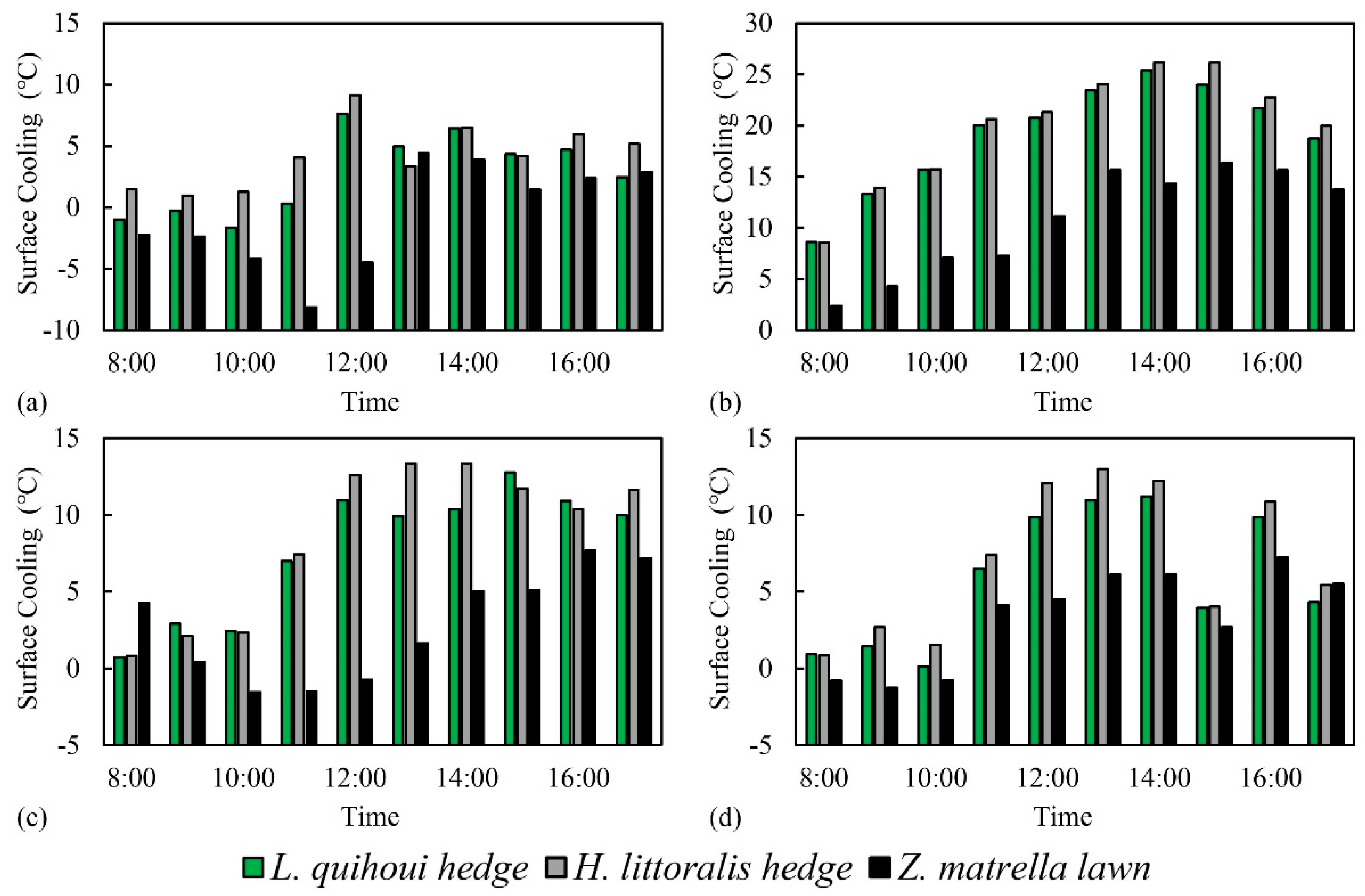
The surface temperature of the asphalt road was higher than the hedges most of the time (Figure 10). The cooling effects of the hedges were more evident in the mid-day, when the underlying surface temperatures were high. During the summer day, the cooling effects on surface temperature could even be over 20 °C between 11:00 a.m. and 4:00 p.m. This means the hedges could significantly reduce the peak surface temperature in a day. The daily average cooling effects of the two hedges during the summer day were 19.17–19.94 °C. They were much weaker on the other three days, especially in the spring day, when the two hedges could only cool the underlying surface by 2.80–4.22 °C. The surface temperature cooling effects were even negative in the morning of the spring day. The low ET rate of the L. quihoui hedge restricted its cooling effect at that time. In addition, the asphalt road dissipated heat in the night before becoming cooler in the morning [59]. As a result, the surface temperature of the road could be lower than the hedge.
The H. littoralis hedge had better cooling effects on underlying surface temperatures than the L. quihoui hedge. The H. littoralis hedge cooled the underlying surface temperature by 4.22, 19.94, 8.57, and 7.00 °C on the four days, respectively. Simultaneously, the L. quihoui hedge could cool the surface by 2.80, 19.17, 7.80, and 5.92 °C. The hedges always showed better cooling effects than the lawn. The cooling effects of the lawn were −0.62, 10.81, 2.75, and 3.36 °C on the four selected days. The most distinct differences of cooling effects between the hedges and the lawn were during the summer day. The hedges could cool the surface by 9 °C more than the lawn. The minimum differences occurred on the winter day, when the two hedges cooled by more 2.56 °C and 3.64 °C than the lawn.
4. Discussion
4.1. The ET Characteristics of Urban Hedges
The ET rates of two common urban hedges were estimated in this study, and both were found to be relatively high. The ET rates of the H. littoralis hedge were 0.04, 0.38, 0.13, and 0.18 mm h−1 during the four typical sunny days from four seasons. The ET rates of the L. quihoui hedge were slightly lower: on the four days selected, they were 0.03, 0.33, 0.09, and 0.17 mm h−1, respectively. The ET rates of the two hedges have also been studied in other cities. A study conducted in Hubei, China showed that the ET rate of H. littoralis (0.04 mm h−1) was higher than that of six other plants in summer [60]. It also found that the H. littoralis had the highest light utilization efficiency and the third highest water use efficiency. Another study conducted in Changsha, China showed that the L. quihoui could transport 2576.52 g·m−2·d−1 (approximately 0.11 mm h−1) of water into the air through ET in August [61]. It was the third highest out of the 13 studied shrubs. However, the ET rates in the two studies above are much lower than our results, as the two previous cities get less solar radiation compared with our study sites.
The winter in Shenzhen is warm enough to sustain plant growth, so almost all local plants are evergreen [62]. As a result, the ET rate of the H. littoralis hedge was still high in the winter day. In addition, with its high light and water utilization efficiency, its ET rate might be slightly higher than that of the L. quihoui hedge. The ET rates of the two hedges were both higher than the ET rates of the lawn. LAI might be the predominant reason [63].
4.2. Cooling Effect of the Urban Hedges
Three techniques were used to describe the cooling effects of the urban hedges in this study. Among them, the cooling effects of plants through ET alone was calculated using a reference method. For 10 cubic meters of air, this H. littoralis hedge could generate cooling at rates of 0.12 °C min−1 m−2, 1.29 °C min−1 m−2, 0.42 °C min−1 m−2, and 0.61 °C min−1 m−2 on the four studied days. Meanwhile, the cooling rates of the L. quihoui hedge were 0.10 °C min−1 m−2, 1.13 °C min−1 m−2, 0.30 °C min−1 m−2, and 0.56 °C min−1 m−2. In our reference research, a 2885-m2 S. superba forest in Guangzhou, another subtropical megacity near Shenzhen, could cool a 10-m3 air column at rates of 0.15 °C min−1 m−2 and 0.13 °C min−1 m−2 in July in 2007 and 2008 [58]. Its cooling rates by per unit area vegetation were lower than our results, as the ET during the day and night in all kinds of weather were included in their study. The daily UHIIs around our study sites over four seasons were approximately 0.76, 1.06, 1.04, and 0.80 °C [64]. For the whole city, the yearly average UHII of Shenzhen was 2.6 °C [65]. Therefore, the urban hedges showed great cooling potential in the mitigation of UHI.
The cooling rate above is the temperature reduction by ET without heat input. The LE/Rn reflects the proportions of the net radiation that ET dissipates. The greater the proportions of net radiation that were consumed by latent heat, the smaller proportion of net radiation could heat the environment through sensible heat. The H. littoralis hedge could consume 37.27%, 68.44%, 56.10%, and 65.71% of the net radiation as latent heat over the four days, while for the L. quihoui hedge the ratios were 35.72%, 60.81%, 41.45%, and 61.58%. These ratios were significantly higher than artificial underlying surfaces. It was found that only 123 Wh m−2 out of the 1949 Wh m−2 net radiation reaching to the asphalt roof was consumed by latent heat [66]. Grimmond et al. reported 23% of the LE/Rn in Marseille, where the area fraction of vegetation and water was 10–20%. Meanwhile, areas like Me93 and Vl92 that contained less vegetation had a lower LE/Rn [67]. In Kansas City, the LE/Rn could reach 46–58% in an exurban residential neighborhood, where the vegetation accounted for 58% of the total area [68]. This phenomenon was also demonstrated in a study conducted in Kugahara, Tokyo, where the LE/Rn in the daytime was always larger in hot months and smaller in cooler months [69]. According to LE/Rn, the H. littoralis hedge had better cooling effects than the L. quihoui hedge. The LE/Rn was larger when the radiation was stronger, which means the cooling effects of ET might be stronger in hotter days.
The albedo differences may result in the surface temperature differences between hedges and asphalt pavements [70,71]. Moreover, the hedges could consume much more heat through ET than artificial underlying surfaces [72]. Compared to the asphalt pavement, the surface temperature of the studied H. littoralis hedge were 4.22, 19.94, 8.57, and 7.00 °C lower on the four days. The surface temperature of the L. quihoui hedge were 2.80, 19.17, 7.80, and 5.92 °C lower at the same time. The forested land could also cool the surface more than 10 °C in November compared with developed land [73]. Leuzinger et al. found that tree canopies in Basel were 19 °C cooler than roofs in July, and different trees had different canopy temperatures [74]. The land surface temperature differences between land use types of transportation and green spaces in Shenzhen were approximately 4.8 °C in daytime in October [75]. In comparison with the studies above, the cooling effects of the urban hedges in our research are remarkable. The amplitudes of the hedges’ surface temperature were also smaller than those of the asphalt road in the daytime, which means the thermal environment was more stable in the urban hedge area (Table 4). Similar results have been found in previous studies [76]. They found that the maximum daily variation of surface temperature was no more than 3 °C, and the maximum surface temperature was only 26.5 °C for Raphis palm, while for the hard surface, they were 30 °C and 57 °C, respectively. Latent heat could significantly reduce the maximum surface temperature in a day but showed minimal effects on the minimum temperature [77].
4.3. Applicability of the ‘3T + IR’ Method for the ET Estimation of Urban Hedges
In this study, a new method based on ‘3T + IR’ was applied to accurately estimate urban ET. The applicability of this method on urban vegetation has been verified in this study by comparison with the BREB method. The results showed great reliability in this new method. With this method, the ET rates of the hedges can be calculated by surface temperature, which could be easily obtained by thermal images. Therefore, this method will not be limited by the complexity of urban underlying surfaces, which is the main obstacle for traditional methods. It also has a higher temporal and spatial resolution than traditional satellite remote sensing. Based on accurate ET rates, the specific cooling effects of ET could be obtained.
In this study, to simplify the calculation and measurement, the emissivity of the hedges and the lawn were defined as 0.98 and the net radiation was estimated based on the solar radiation and temperatures. Therefore, there might be some bias of the results. Besides, the leaf with the highest surface temperature was selected to be the reference leaf. The ET of this leaf actually is larger than zero, therefore will leading a little overestimation of the actually ET of the vegetation based on three-temperature model. Though it has been applied and validated in various field experiments out of the city, this is the first application of this new method in the study of urban hedges. Therefore, more research is needed. For example, an idealized reference leaf is still hard to select. The shape, emissivity and albedo of the reference leaf could affect the results. Besides, this method could not be used in continuous measurement at a high frequency, as we could only photo the thermal images and measure the net radiation by hand. Automatic imaging technique of infrared remote sensing and net radiation measurement will be helpful in the future.
5. Conclusions
In this study, the ET characteristics of two urban hedges were measured by a fetch-free method with high spatiotemporal resolution, namely, the ‘three-temperature model + infrared remote sensing’ method. The method demonstrated high accuracy in the ET estimation for urban vegetation. The results show that: (1) the ET rates of the two studied urban hedges were high. On the summer day, the daily average ET rate of the H. littoralis hedge was 0.38 mm h−1, while that of the L. quihoui hedge was 0.33 mm h−1. (2) The latent heat of the hedges accounts for a large part of the net radiation. The two hedges consumed 68.44% and 60.81% of the net radiation via ET on the summer day. Therefore, the hedges have great cooling potential in the urban thermal environment. (3) The contribution of ET to the vegetation cooling effects in urban areas could be identified through more accurate ET rates. The daily average cooling rates of the two hedges on air temperature through ET alone could reach 1.13–1.29 °C min−1 m−2. (4) The hedges could also significantly cool down the underlying urban surface. The cooling effect was stronger on hotter days. On the hottest day, the cooling effects of the two hedges on the underlying surface were more than 19 °C. (5) The ET rates of the H. littoralis hedge were slightly higher than those of the L. quihoui hedge and therefore had better cooling effects, while both had much better cooling effects than the lawn used for comparison. These results may contribute to the greening design for urban areas.
This study may be the first research that can quantitatively measure the ET rate of urban hedge and provide a new insight to understand the process of ET in urban hedges, and could also promote the methodology of urban ET studies.
Author Contributions
G.Y.Q. designed the research; Z.Z. and Y.Y. carried out the field experiment; Z.Z. made the data analysis and wrote this paper.
Funding
This research was funded by the Special Fund for National Key Research and Development Plan, grant number 2017FY100206-03.
Acknowledgments
The authors would like to express their great thanks to: Chunhua Yan and Yang Zhang for their assistance in the article writing; Wenli Zhao for coding the software “A system to estimate ET by infrared remote sensing and the three-temperature model”; Peng Mao for help in graphics. Elsevier Language Editing for their efforts to improve the grammar of this paper.
Conflicts of Interest
The authors declare no conflict of interest.
References
- Tan, J.; Zheng, Y.; Tang, X.; Guo, C.; Li, L.; Song, G.; Zhen, X.; Yuan, D.; Kalkstein, A.J.; Li, F. The urban heat island and its impact on heat waves and human health in Shanghai. Int. J. Biometeorol. 2010, 54, 75–84. [Google Scholar] [CrossRef]
- Gaffin, S.R.; Rosenzweig, C.; Khanbilvardi, R.; Parshall, L.; Mahani, S.; Glickman, H.; Goldberg, R.; Blake, R.; Slosberg, R.B.; Hillel, D. Variations in New York city’s urban heat island strength over time and space. Theor. Appl. Climatol. 2008, 94, 1–11. [Google Scholar] [CrossRef]
- Ren, G.; Zhou, Y.; Chu, Z.; Zhou, J.; Zhang, A.; Guo, J.; Liu, X. Urbanization Effects on Observed Surface Air Temperature Trends in North China. J. Clim. 2008, 21, 1333–1348. [Google Scholar] [CrossRef]
- Peng, S.; Piao, S.; Ciais, P.; Friedlingstein, P.; Ottle, C.; Bréon, F.M.; Nan, H.; Zhou, L.; Myneni, R.B. Surface urban heat island across 419 global big cities. Environ. Sci. Technol. 2012, 46, 696–703. [Google Scholar] [CrossRef]
- Lin, W.; Wu, T.; Zhang, C.; Yu, T. Carbon savings resulting from the cooling effect of green areas: A case study in Beijing. Environ. Pollut. 2011, 159, 2148–2154. [Google Scholar] [CrossRef]
- Gobakis, K.; Kolokotsa, D.; Synnefa, A.; Saliari, M.; Giannopoulou, K.; Santamouris, M. Development of a model for urban heat island prediction using neural network techniques. Sustain. Cities Soc. 2011, 1, 104–115. [Google Scholar] [CrossRef]
- Gosling, S.N.; Lowe, J.A.; Mcgregor, G.R.; Pelling, M.; Malamud, B.D. Associations between elevated atmospheric temperature and human mortality: A critical review of the literature. Clim. Chang. 2009, 92, 299–341. [Google Scholar] [CrossRef]
- Kinney, P.L. Climate change, air quality, and human health. Am. J. Prev. Med. 2008, 35, 459–467. [Google Scholar] [CrossRef]
- Merte, S. Estimating heat wave-related mortality in Europe using singular spectrum analysis. Clim. Chang. 2017, 142, 321–330. [Google Scholar] [CrossRef]
- Santamouris, M. Cooling the cities—A review of reflective and green roof mitigation technologies to fight heat island and improve comfort in urban environments. Sol. Energy 2014, 103, 682–703. [Google Scholar] [CrossRef]
- Ketterer, C.; Matzarakis, A. Human-biometeorological assessment of heat stress reduction by replanning measures in Stuttgart, Germany. Landsc. Urban Plan. 2014, 122, 78–88. [Google Scholar] [CrossRef]
- Akbari, H.; Pomerantz, M.; Taha, H. Cool surfaces and shade trees to reduce energy use and improve air quality in urban areas. Sol. Energy 2001, 70, 295–310. [Google Scholar] [CrossRef]
- Xu, C.Y.; Chen, D. Comparison of seven models for estimation of evapotranspiration and groundwater recharge using lysimeter measurement data in Germany. Hydrol. Process. 2010, 19, 3717–3734. [Google Scholar] [CrossRef]
- Takebayashi, H.; Moriyama, M. Study on the urban heat island mitigation effect achieved by converting to grass-covered parking. Sol. Energy 2009, 83, 1211–1223. [Google Scholar] [CrossRef] [Green Version]
- Nastran, M.; Kobal, M.; Eler, K. Urban Heat Islands in Relation to Green Land Use in European Cities. Urban For. Urban Green. 2018, in press. [Google Scholar] [CrossRef]
- Imran, H.M.; Kala, J.; Ng, A.W.M.; Muthukumaran, S. Effectiveness of green and cool roofs in mitigating urban heat island effects during a heatwave event in the city of Melbourne in southeast Australia. J. Clean Prod. 2018, 197, 393–405. [Google Scholar] [CrossRef]
- Mariani, L.; Parisi, S.G.; Cola, G.; Lafortezza, R.; Colangelo, G.; Sanesi, G. Climatological analysis of the mitigating effect of vegetation on the urban heat island of Milan, Italy. Sci. Total Environ. 2016, 569–570, 762–773. [Google Scholar] [CrossRef]
- Zheng, S.; Zhao, L.; Li, Q. Numerical simulation of the impact of different vegetation species on the outdoor thermal environment. Urban For. Urban Green. 2016, 18, 138–150. [Google Scholar] [CrossRef]
- Akbari, H.; Dan, M.K.; Bretz, S.E.; Hanford, J.W. Peak power and cooling energy savings of shade trees. Energy Build. 1997, 25, 139–148. [Google Scholar] [CrossRef]
- Ballinas, M.; Barradas, V.L. The Urban Tree as a Tool to Mitigate the Urban Heat Island in Mexico City: A Simple Phenomenological Model. J. Environ. Qual. 2016, 45, 157–166. [Google Scholar] [CrossRef]
- Hamada, S.; Ohta, T. Seasonal variations in the cooling effect of urban green areas on surrounding urban areas. Urban For. Urban Green. 2010, 9, 15–24. [Google Scholar] [CrossRef]
- Feyisa, G.L.; Dons, K.; Meilby, H. Efficiency of parks in mitigating urban heat island effect: An example from Addis Ababa. Landsc. Urban Plan. 2014, 123, 87–95. [Google Scholar] [CrossRef]
- Doick, K.J.; Peace, A.; Hutchings, T.R. The role of one large greenspace in mitigating London’s nocturnal urban heat island. Sci. Total Environ. 2014, 493, 662–671. [Google Scholar] [CrossRef]
- Wong, N.H.; Jusuf, S.K.; Win, A.A.L.; Thu, H.K.; Negara, T.S.; Wu, X. Environmental study of the impact of greenery in an institutional campus in the tropics. Build. Environ. 2007, 42, 2949–2970. [Google Scholar] [CrossRef]
- Weng, Q.; Yang, S. Managing the adverse thermal effects of urban development in a densely populated Chinese city. J. Environ. Manag. 2004, 70, 145–156. [Google Scholar] [CrossRef]
- Dimoudi, A.; Nikolopoulou, M. Vegetation in the urban environment: Microclimatic analysis and benefits. Energy Build. 2003, 35, 69–76. [Google Scholar] [CrossRef]
- Scott, K.I.; Simpson, J.R.; Mcpherson, E.G. Effects of tree cover on parking lot microclimate and vehicle emissions. J. Arboric. 1999, 25, 129–142. [Google Scholar]
- Berthier, E.; Dupont, S.; Mestayer, P.G.; Andrieu, H. Comparison of two evapotranspiration schemes on a sub-urban site. J. Hydrol. 2006, 328, 635–646. [Google Scholar] [CrossRef]
- Lazzarin, R.M.; Castellotti, F.; Busato, F. Experimental measurements and numerical modelling of a green roof. Energy Build. 2005, 37, 1260–1267. [Google Scholar] [CrossRef]
- Qiu, G.; Tan, S.; Wang, Y.; Yu, X.; Yan, C. Characteristics of Evapotranspiration of Urban Lawns in a Sub-Tropical Megacity and Its Measurement by the ‘Three Temperature Model + Infrared Remote Sensing’ Method. Remote Sens. 2017, 9, 502. [Google Scholar] [Green Version]
- Nouri, H.; Glenn, E.; Beecham, S.; Chavoshi Boroujeni, S.; Sutton, P.; Alaghmand, S.; Noori, B.; Nagler, P. Comparing Three Approaches of Evapotranspiration Estimation in Mixed Urban Vegetation: Field-Based, Remote Sensing-Based and Observational-Based Methods. Remote Sens. 2016, 8, 492. [Google Scholar] [CrossRef]
- Pataki, D.E.; Mccarthy, H.R.; Litvak, E.; Pincetl, S. Transpiration of urban forests in the Los Angeles metropolitan area. Ecol. Appl. 2011, 21, 661–677. [Google Scholar] [CrossRef]
- DiGiovanni, K.; Montalto, F.; Gaffin, S.; Rosenzweig, C. Evaluation of Physically and Empirically Based Models for the Estimation of Green Roof Evapotranspiration. J. Hydrol. Eng. 2010, 18, 99–107. [Google Scholar] [CrossRef]
- Qiu, G.Y.; Momii, K.; Yano, T. Estimation of Plant Transpiration by Imitation Leaf Temperature: Theoretical consideration and field verification (I). Trans. Jpn. Soc. Irrig. Drain. Rural Eng. 1996, 64, 401–410. [Google Scholar]
- Qiu, G.Y.; Yano, T.; Momii, K. Estimation of Plant Transpiration by Imitation Leaf Temperature: Application of imitation leaf temperature for detection of crop water stress (II). Trans. Jpn. Soc. Irrig. Drain. Rural Eng. 1996, 64, 767–773. [Google Scholar]
- Wang, Y.Q.; Xiong, Y.J.; Qiu, G.Y.; Zhang, Q.T. Is scale really a challenge in evapotranspiration estimation? A multi-scale study in the Heihe oasis using thermal remote sensing and the three-temperature model. Agric. For. Meteorol. 2016, 230–231, 128–141. [Google Scholar] [CrossRef]
- Tian, F.; Qiu, G.Y.; Lü, Y.H.; Yang, Y.H.; Xiong, Y. Use of high-resolution thermal infrared remote sensing and “three-temperature model” for transpiration monitoring in arid inland river catchment. J. Hydrol. 2014, 515, 307–315. [Google Scholar] [CrossRef]
- Xiong, Y.J.; Qiu, G.Y. Simplifying the revised three-temperature model for remotely estimating regional evapotranspiration and its application to a semi-arid steppe. Int. J. Remote Sens. 2014, 35, 2003–2027. [Google Scholar]
- Xiong, Y.J.; Qiu, G.Y. Estimation of evapotranspiration using remotely sensed land surface temperature and the revised three-temperature model. Int. J. Remote Sens. 2011, 32, 5853–5874. [Google Scholar] [CrossRef]
- Qiu, G.Y.; Benasher, J. Experimental determination of soil evaporation stages with soil surface temperature. Soil Sci. Soc. Am. J. 2010, 74, 13–22. [Google Scholar] [CrossRef]
- Qiu, G.Y.; Zhao, M. Remotely monitoring evaporation rate and soil water status using thermal imaging and “three-temperatures model (3T model)” under field-scale conditions. J. Environ. Monit. 2010, 12, 716–723. [Google Scholar] [CrossRef]
- Qiu, G.Y.; Li, C.; Yan, C. Characteristics of soil evaporation, plant transpiration and water budget of Nitraria dune in the arid Northwest China. Agric. For. Meteorol. 2015, 203, 107–117. [Google Scholar] [CrossRef]
- Qiu, G.Y.; Miyamoto, K.; Sase, S.; Okushima, L. Detection of crop transpiration and water stress by temperature-related approach under field and greenhouse conditions. JARQ Jpn. Agric. Res. Q. 2000, 34, 29–37. [Google Scholar]
- Cao, L.; Zhang, Y.; Lu, H.; Yuan, J.; Zhu, Y.; Liang, Y. Grass hedge effects on controlling soil loss from concentrated flow: A case study in the red soil region of China. Soil Tillage Res. 2015, 148, 97–105. [Google Scholar] [CrossRef]
- Forman, R.T.T.; Baudry, J. Hedgerows and hedgerow networks in landscape ecology. Environ. Manag. 1984, 8, 495–510. [Google Scholar] [CrossRef]
- Gosling, L.; Sparks, T.H.; Araya, Y.; Harvey, M.; Ansine, J. Differences between urban and rural hedges in England revealed by a citizen science project. BMC Ecol. 2016, 16 (Suppl. 1), 45–55. [Google Scholar] [CrossRef]
- Gromke, C.; Jamarkattel, N.; Ruck, B. Influence of roadside hedgerows on air quality in urban street canyons. Atmos. Environ. 2016, 139, 75–86. [Google Scholar] [CrossRef]
- Yan, C.; Qiu, G.Y. The three-temperature model to estimate evapotranspiration and its partitioning at multiple scales: A review. Trans. ASABE 2016, 59, 661–670. [Google Scholar]
- Jensen, M.E.; Burman, R.D.; Allen, R.G. Evapotranspiration and irrigation water requirements. In Manuals and Reports on Engineering Practice No. 70; American Society of Civil Engineers: New York, NY, USA, 1990; pp. 25–41. [Google Scholar]
- Weiss, A. An Experimental Study of Net Radiation, Its Components and Prediction. Agron. J. 1982, 74, 871–874. [Google Scholar] [CrossRef]
- Burman, R.D.; Cuenca, R.H.; Weiss, A. Techniques for estimating irrigation water requirements. In Advances in Irrigation; Elsevier: New York, NY, USA, 1983; Volume 2, pp. 335–394. [Google Scholar]
- Hatfield, J.L.; Reginato, R.J.; Idso, S.B. Comparison of long-wave radiation calculation methods over the United States. Water Resour. Res. 1983, 19, 285–288. [Google Scholar] [CrossRef]
- Bowen, I.S. The Ratio of Heat Losses by Conduction and by Evaporation from any Water Surface. Phys Rev. 1926, 27, 779–787. [Google Scholar] [CrossRef] [Green Version]
- Meteorological Bureau of Shenzhen Municipality. Available online: http://www.szmb.gov.cn/qixiangfuwu/qihoufuwu/qihouguanceyupinggu/qihougaikuang/201711/t20171109_9584854.htm (accessed on 5 December 2018).
- Anjos, M.; Lopes, A. Urban Heat Island and Park Cool Island Intensities in the Coastal City of Aracaju, North-Eastern Brazil. Sustainability 2017, 9, 1379. [Google Scholar] [CrossRef]
- Shiflett, S.A.; Liang, L.L.; Crum, S.M.; Feyisa, G.L.; Wang, J.; Jenerette, G.D. Variation in the urban vegetation, surface temperature, air temperature nexus. Sci. Total Environ. 2017, 579, 495–505. [Google Scholar] [CrossRef]
- Park, J.; Kim, J.H.; Dong, K.L.; Park, C.Y.; Jeong, S.G. The influence of small green space type and structure at the street level on urban heat island mitigation. Urban For. Urban Green. 2016, 21, 203–212. [Google Scholar] [CrossRef]
- Zhu, L.W.; Zhao, P. Temporal Variation in Sap-Flux-Scaled Transpiration and Cooling Effect of a Subtropical Schima superba Plantation in the Urban Area of Guangzhou. J. Integr. Agric. 2013, 12, 1350–1356. [Google Scholar] [CrossRef]
- Mohan, M.; Kandya, A. Impact of urbanization and land-use/land-cover change on diurnal temperature range: A case study of tropical urban airshed of India using remote sensing data. Sci. Total Environ. 2015, 506–507, 453–465. [Google Scholar] [CrossRef]
- Zhang, X.J.; De-Ming, L.I.; Zhai, K.R. Study on Light and Water Utilization Characteristics of Several Ground Cover Plants. North Hortic. 2010, 12, 75–78, (In Chinese with English Abstract). [Google Scholar]
- Zhu, Y.Q.; Yang, B.S.; Ya-Xin, Y.U.; Jin, X.L. Comparison of temperature decrease and humidity increase effect of familiar shrub species in Changsha City. Guangdong Agric. Sci. 2013, 9, 42–45, (In Chinese with English Abstract). [Google Scholar]
- Liu, Y.; Peng, J.; Wang, Y. Diversification of Land Surface Temperature Change under Urban Landscape Renewal: A Case Study in the Main City of Shenzhen, China. Remote Sens. 2017, 9, 919. [Google Scholar] [CrossRef]
- Saadatian, O.; Sopian, K.; Salleh, E.; Lim, C.H.; Riffat, S.; Saadatian, E.; Toudeshki, A.; Sulaiman, M.Y. A review of energy aspects of green roofs. Renew. Sustain. Energy Rev. 2013, 23, 155–168. [Google Scholar] [CrossRef]
- Qiu, G.Y.; Zou, Z.; Li, X.; Li, H.; Guo, Q.; Yan, C.; Tan, S. Experimental studies on the effects of green space and evapotranspiration on urban heat island in a subtropical megacity in China. Habitat Int. 2017, 68, 30–42. [Google Scholar] [CrossRef]
- Zhang, E.J.; Zhang, J.J.; Zhao, X.Y.; Zhang, X.L. Study on urban heat island effect in Shenzhen. J. Nat. Disasters 2008, 17, 19–24, (In Chinese with English Abstract). [Google Scholar]
- Schmidt, M.; Tu-Berlin, D.I. The interaction between water and energy of greened roofs. In Proceedings of the World Green Roof Congress, Basel, Switzerland, 15–16 September 2005. [Google Scholar]
- Grimmond, C.S.B.; Salmond, J.A.; Oke, T.R.; Offerle, B.; Lemonsu, A. Flux and turbulence measurements at a densely built-up site in Marseille: Heat, mass (water and carbon dioxide), and momentum. J. Geophys. Res. 2004, 109, D24101. [Google Scholar] [CrossRef]
- Balogun, A.A.; Adegoke, J.O.; Vezhapparambu, S.; Mauder, M.; Mcfadden, J.P.; Gallo, K. Surface Energy Balance Measurements Above an Exurban Residential Neighbourhood of Kansas City, Missouri. Bound.-Layer Meteor. 2009, 133, 299–321. [Google Scholar] [CrossRef] [Green Version]
- Moriwaki, R.; Kanda, M. Seasonal and diurnal fluxes of radiation, heat, water vapor and carbon dioxide over a suburban area. J. Appl. Meteorol. 2004, 43, 1700–1710. [Google Scholar] [CrossRef]
- Blok, D.; Schaepmanstrub, G.; Bartholomeus, H.; Heijmans, M.M.P.D.; Maximov, T.C.; Berendse, F. The response of Arctic vegetation to the summer climate: Relation between shrub cover, NDVI, surface albedo and temperature. Environ. Res. Lett. 2011, 6, 035502. [Google Scholar] [CrossRef]
- Prado, R.T.A.; Ferreira, F.L. Measurement of albedo and analysis of its influence the surface temperature of building roof materials. Energy Build. 2005, 37, 295–300. [Google Scholar] [CrossRef]
- Crawford, A.J.; Mclachlan, D.H.; Hetherington, A.M.; Franklin, K.A. High temperature exposure increases plant cooling capacity. Curr. Biol. 2012, 22, R396–R397. [Google Scholar] [CrossRef] [Green Version]
- Xie, M.; Wang, Y.; Meichen, F.U.; Zhang, D. Pattern Dynamics of Thermal-environment Effect During Urbanization: A Case Study in Shenzhen City, China. Chin. Geogr. Sci. 2013, 23, 101–112, (In Chinese with English Abstract). [Google Scholar] [CrossRef]
- Leuzinger, S.; Vogt, R.; Körner, C. Tree surface temperature in an urban environment. Agric. For. Meteorol. 2010, 150, 56–62. [Google Scholar] [CrossRef]
- Chen, Z.; Gong, C.; Wu, J.; Yu, S. The influence of socioeconomic and topographic factors on nocturnal urban heat islands: A case study in Shenzhen, China. Int. J. Remote Sens. 2012, 33, 3834–3849. [Google Scholar] [CrossRef]
- Wong, N.H.; Chen, Y.; Ong, C.L.; Sia, A. Investigation of thermal benefits of rooftop garden in the tropical environment. Build. Environ. 2003, 38, 261–270. [Google Scholar] [CrossRef]
- Yang, Y.; Ren, R. On the Contrasting Decadal Changes of Diurnal Surface Temperature Range between the Tibetan Plateau and Southeastern China during the 1980s–2000s. Adv. Atmos. Sci. 2017, 34, 181–198. [Google Scholar] [CrossRef]
Figure 1.
Location of the study area. The upper left figure is the location of Shenzhen City. The upper right figure shows the location of the study area in Shenzhen. The bottom figure is a photo of the studied area by google earth. The studied hedges and lawn are in the red box.
Figure 1.
Location of the study area. The upper left figure is the location of Shenzhen City. The upper right figure shows the location of the study area in Shenzhen. The bottom figure is a photo of the studied area by google earth. The studied hedges and lawn are in the red box.
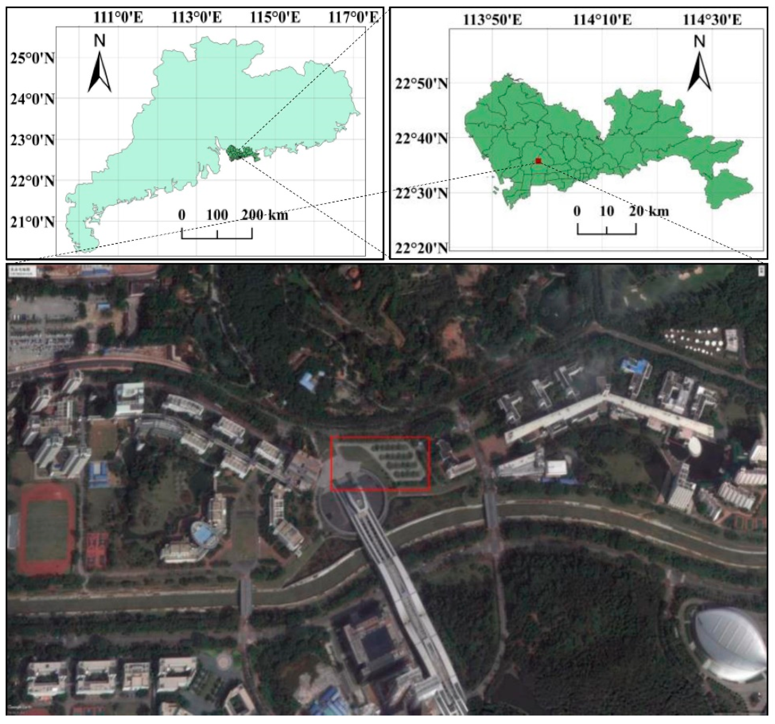
Figure 2.
Comparison of the ET rates of urban vegetation estimated by the ‘3T + IR’ method and BREB method. 3T + IR: three-temperature model + infrared remote sensing; BREB: Bowen ratio energy balance; ET3: ET rate measured by ‘3T + IR’ method; ETB: ET rate measured by the BREB method.
Figure 2.
Comparison of the ET rates of urban vegetation estimated by the ‘3T + IR’ method and BREB method. 3T + IR: three-temperature model + infrared remote sensing; BREB: Bowen ratio energy balance; ET3: ET rate measured by ‘3T + IR’ method; ETB: ET rate measured by the BREB method.

Figure 3.
Characteristics of weather in the typical sunny days during each season in the study area. (a) the air temperature; (b) the relative humidity; (c) the solar radiation; (d) the wind velocity. Data were measured by the Bowen ratio system in 22 August 2015 (Summer); 18 December 2015 (Autumn); 4 February 2016 (Winter); and 19 March 2016 (Spring). The air temperature and relative humidity are the average of the values measured at 1.5 m and 2.0 m.

Figure 4.
The surface temperatures (K) and ET rates (mm h−1) of the two hedges at 12:00 p.m. in 22 August 2015. (a) the surface temperature of the L. quihoui hedge; (b) the ET rates of the L. quihoui hedge; (c) the surface temperature of the H. littoralis hedge; (d) the ET rates of the H. littoralis hedge. The ET rates were calculated by our software based on the ‘3T + IR’ method and plotted by ArcGIS.

Figure 5.
Surface temperature of the hedges and the lawn for comparison over the four days (the temperatures were the average values of three images. (a) Spring: 19 March 2016; (b) Summer: 22 August 2015; (c) Autumn: 18 December 2015; (d) Winter: 4 February 2016).
Figure 5.
Surface temperature of the hedges and the lawn for comparison over the four days (the temperatures were the average values of three images. (a) Spring: 19 March 2016; (b) Summer: 22 August 2015; (c) Autumn: 18 December 2015; (d) Winter: 4 February 2016).

Figure 6.
ET rates of the hedges and the lawn for comparison on the four typical sunny days in four seasons. (a) Spring: 19 March 2016; (b) Summer: 22 August 2015; (c) Autumn: 18 December 2015; (d) Winter: 4 February 2016.
Figure 6.
ET rates of the hedges and the lawn for comparison on the four typical sunny days in four seasons. (a) Spring: 19 March 2016; (b) Summer: 22 August 2015; (c) Autumn: 18 December 2015; (d) Winter: 4 February 2016.

Figure 7.
Latent heat flux of the hedges and the lawn for comparison on the four typical sunny days in four seasons. The latent heat flux was figured out directly from the three-temperature model. The LE/Rn is the proportion of the latent heat to the net radiation. (a) Spring: 19 March 2016; (b) Summer: 22 August 2015; (c) Autumn: 18 December 2015; (d) Winter: 4 February 2016.
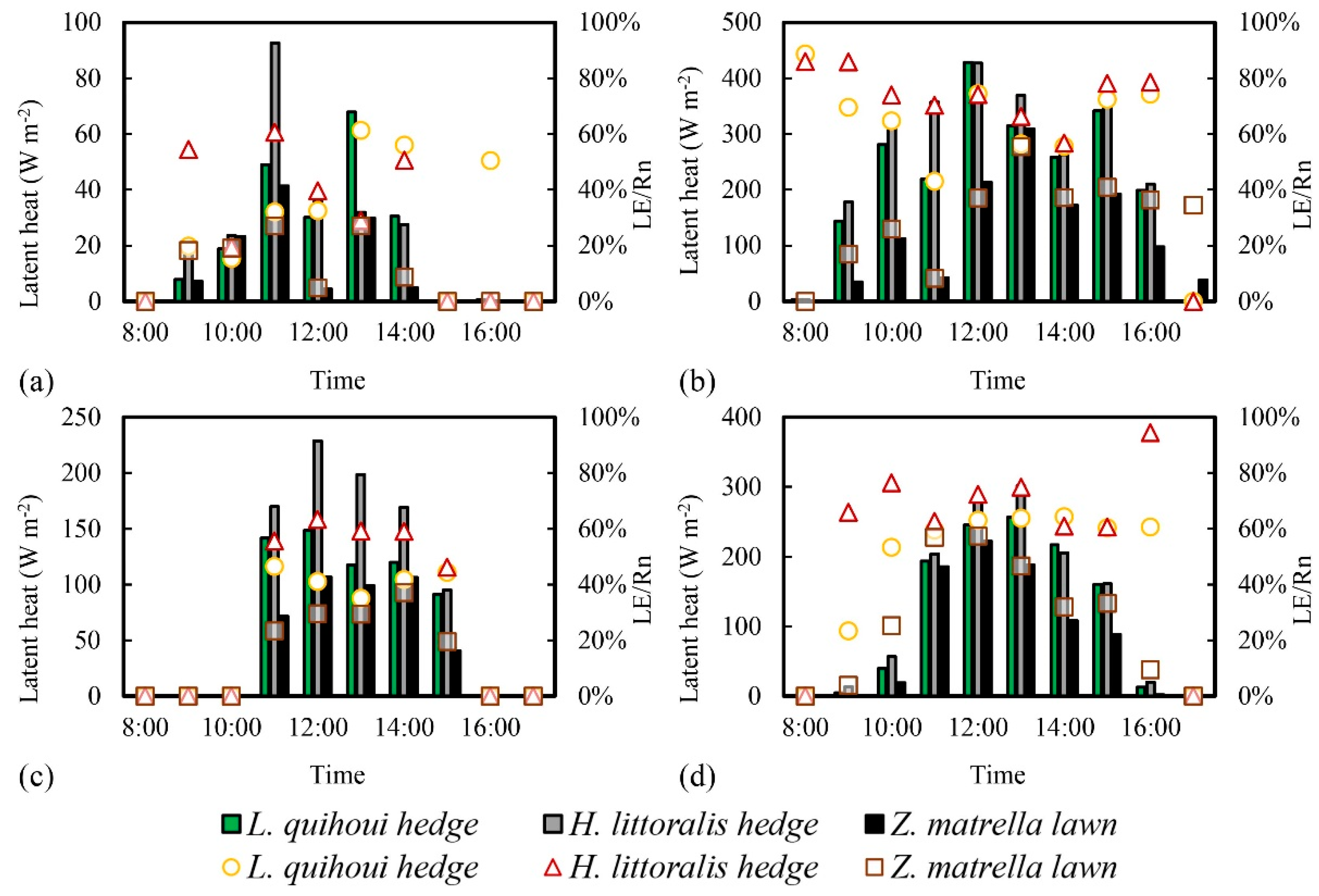
Figure 8.
The cooling rates of hedges and the lawn for comparison on air temperature on the four typical sunny days in four seasons. (a) Spring: 19 March 2016; (b) Summer: 22 August 2015; (c) Autumn: 18 December 2015; (d) Winter: 4 February 2016.
Figure 8.
The cooling rates of hedges and the lawn for comparison on air temperature on the four typical sunny days in four seasons. (a) Spring: 19 March 2016; (b) Summer: 22 August 2015; (c) Autumn: 18 December 2015; (d) Winter: 4 February 2016.

Figure 9.
Surface temperature of the asphalt road in the four typical days in four seasons. Spring: 19 March 2016; Summer: 22 August 2015; Autumn: 18 December 2015; Winter: 4 February 2016.
Figure 9.
Surface temperature of the asphalt road in the four typical days in four seasons. Spring: 19 March 2016; Summer: 22 August 2015; Autumn: 18 December 2015; Winter: 4 February 2016.
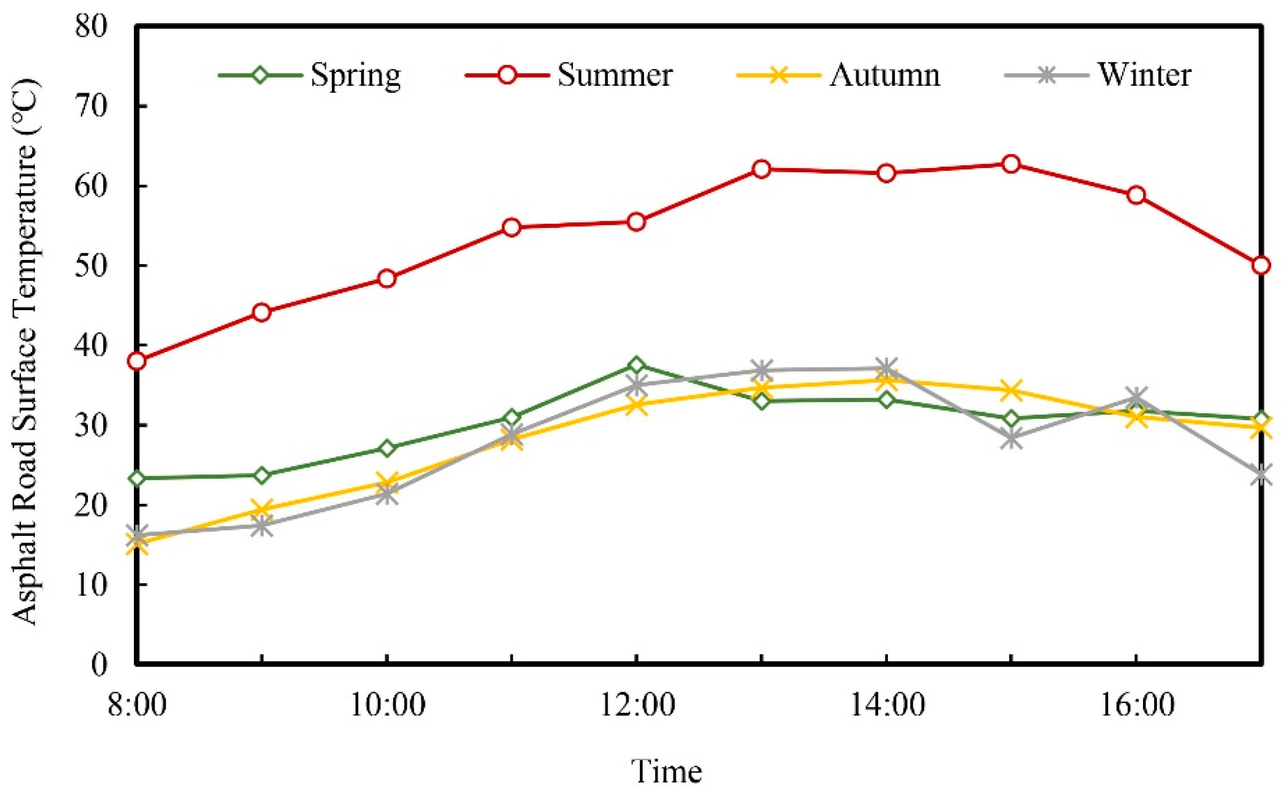
Figure 10.
Surface temperature differences between the hedges, lawn and asphalt pavement on the four typical sunny days in four seasons. (a) Spring: 19 March 2016; (b) Summer: 22 August 2015; (c) Autumn: 18 December 2015; (d) Winter: 4 February 2016.
Figure 10.
Surface temperature differences between the hedges, lawn and asphalt pavement on the four typical sunny days in four seasons. (a) Spring: 19 March 2016; (b) Summer: 22 August 2015; (c) Autumn: 18 December 2015; (d) Winter: 4 February 2016.

Table 1.
Type of sensor, measurement height, and resolutions of the equipment in the Bowen ratio system.
Table 1.
Type of sensor, measurement height, and resolutions of the equipment in the Bowen ratio system.
| Parameter | Sensor Type | Measuring Height(m) | Sensor Resolution |
|---|---|---|---|
| Humidity and Air Temperature | 225-050YA, Novalynx, Grass Valley, CA, USA | 2.0; 1.5 | ±3%, ±0.6 °C |
| Wind Velocity | 200-WS-02, Novalynx, Grass Valley, CA, USA | 2.0 | ±0.2 m s−1 |
| Solar Radiation | PYP-PA, Apogee, Santa Monica, CA, USA | 2.0 | 10–40 μV/W/m2 |
| Net Radiation | 240-100, Novalynx, Grass Valley, CA, USA | 2.0 | <4% |
| Soil Heat Flux | HFP01, Hukseflux, Center Moriches, NY, USA | −0.05; −0.02 | 50 μV/W/m2 |
Table 2.
Average ET rates (mm h−1) of the hedges and the lawn for comparison on the four typical sunny days in four seasons. Spring: 19 March 2016; Summer: 22 August 2015; Autumn: 18 December 2015; Winter: 4 February 2016.
Table 2.
Average ET rates (mm h−1) of the hedges and the lawn for comparison on the four typical sunny days in four seasons. Spring: 19 March 2016; Summer: 22 August 2015; Autumn: 18 December 2015; Winter: 4 February 2016.
| Seasons | H. littoralis Hedge | L. quihoui Hedge | Z. matrella Lawn |
|---|---|---|---|
| Spring | 0.04 | 0.03 | 0.02 |
| Summer | 0.38 | 0.33 | 0.18 |
| Autumn | 0.13 | 0.09 | 0.06 |
| Winter | 0.18 | 0.17 | 0.12 |
Table 3.
Daily average LE/Rn of the hedges and the lawn for comparison on the four typical sunny days in four seasons. Spring: 19 March 2016; Summer: 22 August 2015; Autumn: 18 December 2015; Winter: 4 February 2016.
Table 3.
Daily average LE/Rn of the hedges and the lawn for comparison on the four typical sunny days in four seasons. Spring: 19 March 2016; Summer: 22 August 2015; Autumn: 18 December 2015; Winter: 4 February 2016.
| Seasons | H. littoralis Hedge | L. quihoui Hedge | Z. matrella Lawn |
|---|---|---|---|
| Spring | 37.27% | 35.72% | 28.23% |
| Summer | 68.44% | 60.81% | 39.52% |
| Autumn | 56.10% | 41.45% | 34.06% |
| Winter | 65.71% | 61.58% | 47.28% |
Table 4.
Standard deviations of the surface temperatures on the four days (°C).
| Underlying Surface | Spring | Summer | Autumn | Winter |
|---|---|---|---|---|
| Asphalt pavement | 4.18 | 7.90 | 6.65 | 7.43 |
| H. littoralis hedge | 2.22 | 2.85 | 2.43 | 3.46 |
| L. quihoui hedge | 2.06 | 3.14 | 3.14 | 3.69 |
| Z. matrella lawn | 5.16 | 4.19 | 6.71 | 5.04 |
© 2019 by the authors. Licensee MDPI, Basel, Switzerland. This article is an open access article distributed under the terms and conditions of the Creative Commons Attribution (CC BY) license (http://creativecommons.org/licenses/by/4.0/).
Share and Cite
MDPI and ACS Style
Zou, Z.; Yang, Y.; Qiu, G.Y. Quantifying the Evapotranspiration Rate and Its Cooling Effects of Urban Hedges Based on Three-Temperature Model and Infrared Remote Sensing. Remote Sens. 2019, 11, 202. https://doi.org/10.3390/rs11020202
AMA Style
Zou Z, Yang Y, Qiu GY. Quantifying the Evapotranspiration Rate and Its Cooling Effects of Urban Hedges Based on Three-Temperature Model and Infrared Remote Sensing. Remote Sensing. 2019; 11(2):202. https://doi.org/10.3390/rs11020202
Chicago/Turabian StyleZou, Zhendong, Yajun Yang, and Guo Yu Qiu. 2019. "Quantifying the Evapotranspiration Rate and Its Cooling Effects of Urban Hedges Based on Three-Temperature Model and Infrared Remote Sensing" Remote Sensing 11, no. 2: 202. https://doi.org/10.3390/rs11020202
Note that from the first issue of 2016, this journal uses article numbers instead of page numbers. See further details here.