Heat Flux Sources Analysis to the Ross Ice Shelf Polynya Ice Production Time Series and the Impact of Wind Forcing

Abstract

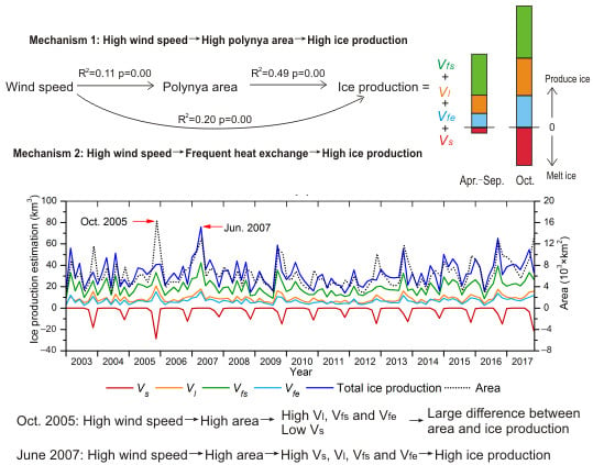
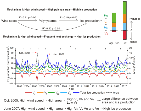
The variation of Ross Ice Shelf Polynya (RISP) ice production is a synergistic result of several factors. This study aims to analyze the 2003–2017 RISP ice production time series with respect to the impact of wind forcing on heat flux sources. RISP ice production was estimated from passive microwave sea ice concentration images and reanalysis meteorological data using a thermodynamic model. The total ice production was divided into four components according to the amount of ice produced by different heat fluxes: solar radiation component (V_s), longwave radiation component (V_l), sensible heat flux component (V_fs), and latent heat flux component (V_fe). The results show that V_fs made the largest contribution, followed by V_l and V_fe, while V_s had a negative contribution. Our study reveals that total ice production and V_l, V_fs, and V_fe highly correlated with the RISP area size, whereas V_s negatively correlated with the RISP area size in October, and had a weak influence from April to September. Since total ice production strongly correlates with the polynya area and this significantly correlates with the wind speed of the previous day, strong wind events lead to sharply increased ice production most of the time. Strong wind events, however, may only lead to mildly increasing ice production in October, when enlarged V_s reduces the ice production. Wind speed influences ice production by two mechanisms: impact on polynya area, and impact on heat exchange and phase transformation of ice. V_fs and V_fe are influenced by both mechanisms, while V_s and V_l are only influenced by impact on polynya area. These two mechanisms show different degrees of influence on ice production during different periods. Persistent offshore winds were responsible for the large RISP area and high ice production in October 2005 and June 2007.

1. Introduction

Polynyas are isolated open water areas surrounded by ice packs [1]. Coastal polynyas, also known as latent heat polynyas, are formed by divergent ice motion, and are driven and maintained by prevailing winds or oceanic currents. Active sea ice formation is found in coastal polynyas, along with brine rejection, which produces dense water [2,3]. The Ross Ice Shelf Polynya (RISP) is the largest coastal polynya over the Southern Ocean, with the highest sea ice production [4,5]. It has been regarded as an important source of Antarctic bottom water [6,7]. Polynya formation and ice production are related to a variety of environmental factors, including atmospheric forcing, currents, tides, air and ocean temperature, landfast ice, and iceberg drift [1,8,9,10,11].

There are two typical ways to estimate polynya ice production: tracing ice motion and energy model simulation. Kwok, Drucker et al., and Comiso et al. [12,13,14] traced ice motion from passive microwave observations and synthetic aperture radar (SAR) imagery. With ice motion data, the sea ice area flux through the polynya was estimated, and the ice production volume was obtained by multiplying the ice area by the ice thickness. Thermodynamic energy models were applied to the polynya surface with atmospheric reanalysis data to simulate the surface energy fluxes [4,15,16,17]. Some researchers also considered the feedback of polynyas to the atmospheric boundary layer. For example, Ebner et al. [18] and Bauer et al. [19] examined the polynya surface energy fluxes with the mesoscale weather prediction model of the Consortium for Small-scale Modeling (COSMO).

The energy model simulation provides an efficient way to separate the individual heat flux components and conduct heat flux sources analysis. First, the polynya area is identified by applying a threshold of sea ice thickness [10,20,21], ice concentration [22,23], or ice classification [5,9,24]. Then the polynya area is combined with a specific source of surface heat flux, and the ice thus produced can be estimated. Woert [25] investigated the correlation between heat flux components and the Terra Nova Bay polynya extent between 1988 and 1990. Ohshima et al. [26] applied a surface heat budget to the Okhotsk Sea, and summarized the seasonal variation of heat flux components. Haid and Timmermann [27] assessed the contribution of heat flux components to polynya ice production in the southwestern Weddell Sea.

The trend of polynya ice production in the Ross Sea has been discussed in previous research [10,13,14,17,21,28]. Martin [10], Nakata [28], and Cheng [17] reported no obvious annual trend of ice production in the Ross Sea since the 2000s. Comiso et al. [14] and Drucker et al. [13] extended the record back to 1992, and reported increasing ice production of about 20 km³/year during 1992–2008. A study by Tamura et al. [21] indicates that RISP ice production demonstrated substantial fluctuations, with a decreasing trend during 1992–2013. Thus, the annual ice production was still hard to predict according to the dynamic change rates. As for seasonal variation, all previous studies reported largely irregular ice production in winter. Heat flux sources analysis, therefore, can provide insight explaining the seasonal and annual variation of ice production.

In this study, we conducted a time series analysis to the Ross Ice Shelf Polynya (RISP) ice production and heat flux components, and examined their response to extreme wind events. We analyzed the daily 2003–2017 ice production time series using ice concentration images and reanalysis atmospheric data. The total ice production was divided into four components according to heat flux sources. The contributions of four components to total ice production were quantified. To explain annual and seasonal ice production variation, we estimated the correlations between polynya area and the production from the four components. Local daily wind speed time series were compared with ice production and four components to reveal the impact of extreme wind forcing. We also performed a comparison between spatial distribution of wind forcing and ice production during two typical periods to visualize their correlations.

2. Methods and Materials

2.1. Polynya Area

In this study, the polynya extent was defined as the sea area with a sea ice concentration (SIC) of less than 75% [29]. We assume that each pixel within the polynya extent is divided into an open water fraction and an ice pack fraction according to the local SIC, and that heat exchange only occurs in the open water fraction. Polynya area refers to the open water fraction within the polynya extent. The polynya area at one pixel is then calculated as

$$Polynya area=\left(1-SIC\right)\times A$$

(1)

where $A$ (= 6.25 × 6.25 km²) is the pixel size. The RISP area is then the sum of the polynya areas within the defined study area.

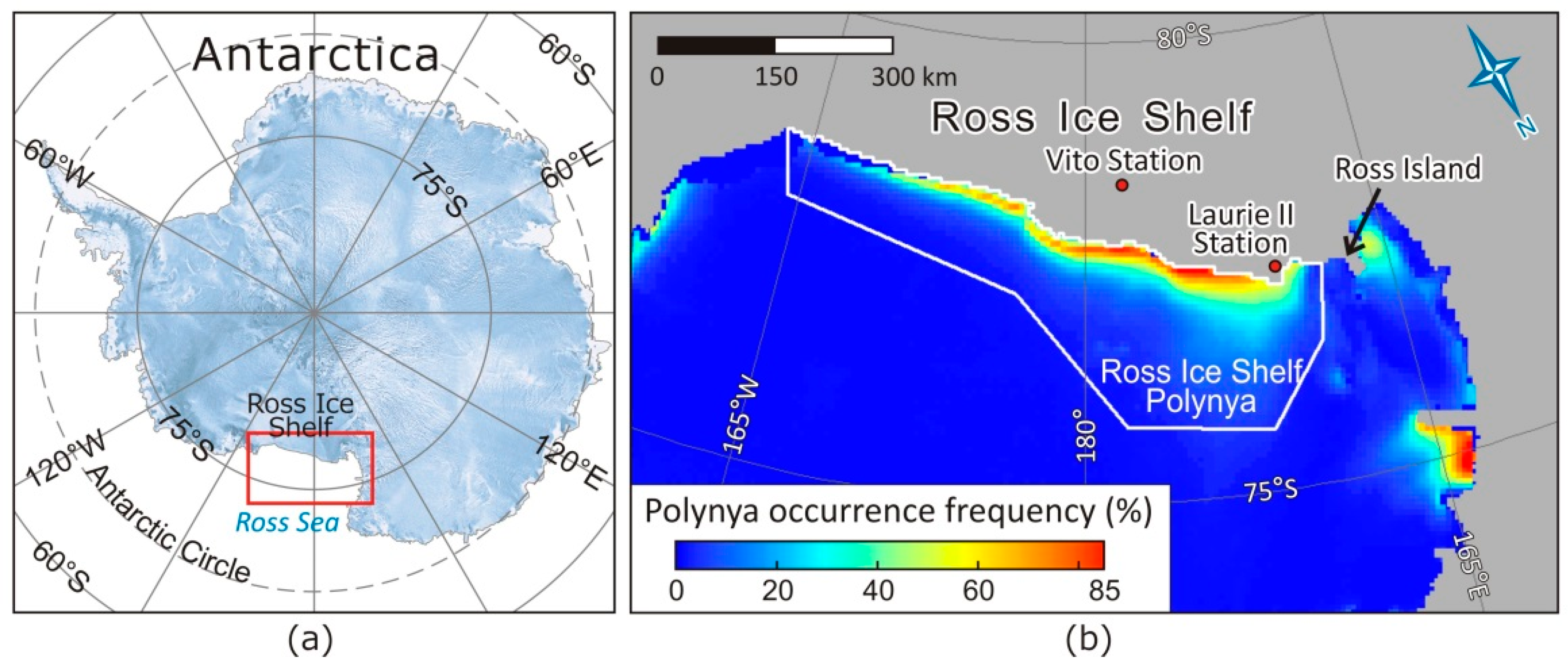
The study area and period were defined by the same method introduced in Cheng et al. [17]. The study period was limited to April–October, 2003–2017, as polynyas only occur in winter. The location of the study area is shown in Figure 1. We defined the study area by a polygon that encloses all pixels with an RISP occurrence frequency >10% (indicated in Figure 1b by the white line).

2.2. Estimation of Ice Production and Heat Flux Components

Ice production was estimated following Cheng et al. [17]. First, the net heat flux $Q$ (in W·m⁻²) on the ocean‒atmosphere interface within the RISP area was estimated, including four components: net solar radiation $S$ (in W·m⁻²), net longwave radiation $L$ (in W·m⁻²), sensible heat flux $F_s$ (in W·m⁻²), and latent heat flux $F_e$ (in W·m⁻²):

$$Q=S+L+F_s+F_e$$

(2)

The parameterization of $S$, $L$, $F_s$, and $F_e$ is described in detail in [17]. Six spatial variables were obtained from reanalysis meteorological data, including air temperature at a height of 2 m, wind speed at a height of 10 m, surface air pressure, dew point temperature of the air at a height of 2 m, incoming solar radiation (S_i), and incoming longwave radiation (L_i). Any oceanic heat flux from below was neglected as coastal polynyas occur in shallow water. S and L are given by

$$S=\left(1-\alpha \right)S_i$$

(3)

$$L=L_i-L_o$$

(4)

$$L_o=\epsilon \sigma T_0^4,$$

(5)

where α (= 0.06) is the albedo of open water. The net solar radiation S is the incoming solar radiation on the ocean surface (S_i) minus the solar radiation reflected by the ocean surface. S_i is acquired from the reanalysis dataset. The net longwave radiation L is the incoming longwave radiation on the ocean surface (L_i) minus the outgoing longwave radiation (L_o). L_i is acquired from the reanalysis dataset. L_o is calculated by the Stefan–Boltzmann law. T₀ (= 271.27 K) is the freezing point of seawater, which is assumed to be the surface temperature of the ocean. $\epsilon$ (= 0.99) is the longwave emissivity of open water, and $\sigma$ (= 5.67 × 10⁻⁸ W·m⁻²·K⁻⁴) is the Stefan–Boltzmann constant.

The net heat flux $Q$ is transformed to ice production $V$ (in m³):

$$V=tA\left(1-SIC\right)Q/{\rho }_i{L}_f,$$

(6)

where $t$ (= 86,400 s) is the number of seconds of one day, ${\rho }_i$ (= 920 kg·m⁻³) is the sea ice density, and $L_f$ (= 2.79 × 10⁵ J·kg⁻¹) is the latent heat of sea ice fusion.

$V$ can be divided into four components according to the heat flux sources, by substituting Equation (2) into Equation (6):

$$V=\frac{tA\left(1-SIC\right)S}{{\rho }_i{L}_f}+\frac{tA\left(1-SIC\right)L}{{\rho }_i{L}_f}+\frac{tA\left(1-SIC\right)F_s}{{\rho }_i{L}_f}+\frac{tA\left(1-SIC\right)F_e}{{\rho }_i{L}_f}=V_s+V_l+V_{fs}+V_{fe}$$

(7)

where V_s, V_l, V_fs, V_fe (in m³) are the amount of ice produced by solar radiation, longwave radiation, sensible heat flux, and latent heat flux, respectively.

2.3. Data

2.3.1. ECMWF Meteorological Data

The input meteorological data were obtained from ERA-Interim, a reanalysis dataset produced by the ECMWF (European Centre for Medium-Range Weather Forecasts) [30]. It contained six input variables: air temperature at a height of 2 m, wind speed at a height of 10 m, surface air pressure, dew point temperature of the air at a height of 2 m, incoming solar radiation, and incoming longwave radiation. All variables were downloaded at a 6 h or 12 h time resolution. They were pre-processed to daily images by arithmetical averaging. The spatial resolution of the downloaded data was 0.125°, which was obtained by interpolating the N128 Gaussian grid. To match the resolution of SIC images, all meteorological images were reprojected onto the same grid as the SIC images.

2.3.2. AWS Wind Forcing Data

ECMWF wind forcing data were compared with Automatic Weather Stations (AWS) wind forcing data, provided by the University of Wisconsin-Madison Automatic Weather Station Program [31]. AWS wind speeds measured at the Vito station and Laurie II station (located in Figure 1b) were utilized. The Vito station was located at 78.408°S, 177.829°E, near the middle of the Ross Ice Shelf edge and the Laurie II station on 77.439°S, 170.750°E, at the west end of RISP, near Ross Island. The Vito station has provided wind speed data since 2004, but includes many time gaps or errors, for example in 2004, September 2007, October 2008, June–July 2010, September–October 2011, and September–October 2012 and 2015. The Laurie II station provided continuous data throughout our study period. The temporal resolution of the downloaded AWS data equals 10 min; they were averaged to daily values.

2.3.3. Sea Ice Concentration (SIC) Maps

The daily SIC maps were provided by the University of Bremen [32,33]. They were retrieved from passive microwave data by using the ASI algorithm, and provided an SIC time series ranging from 2003 to 2017. The full time series was covered by data acquired from the AMSR-E (Advanced Microwave Scanning Radiometer for Earth Observe System), SSMIS (Special Sensor Microwave Imager and Sounder) and AMSR2 (Advanced Microwave Scanning Radiometer 2) sensors. The AMSR-E sensor covers the period from April 2003 to September 2011, the SSMIS sensor covers the period from October 2011 to July 2012, and the AMSR2 sensor covers the period from August 2012 to October 2017. The researchers of the University of Bremen resampled all SIC images to a 6.25 × 6.25 km² grid in the polar-stereographic projection with 70°S standard parallel, although the spatial resolution of the three sensors were different. For example, the 91.0 GHz channel of SSMIS only allows for resolution of 12.5 km.

Some missing dates were filled: the missing images from 30 October 2003 and 31 October 2003 were replaced by those of 29 October 2003, those of 11 May 2013 to 14 May 2013 were replaced by the average image of 10 May 2013 and 15 May 2013, and the image of 28 September 2017 was replaced by the average of 27 September 2017 and 29 September 2017.

2.3.4. Landmasks

Landmasks were used to exclude areas of lands and ice shelves. Kern et al. [5,34] provided landmasks updated every other year until 2008 in their Antarctic polynya products. We overlaid these landmasks on SIC maps from 2003 to 2008. The National Snow and Ice Data Center (NSIDC) [35] provided a landmask image updated in 2009 and 2010. We overlaid this landmask on SIC maps from 2009 to 2017.

3. Results

3.1. The RISP Ice Production Time Series

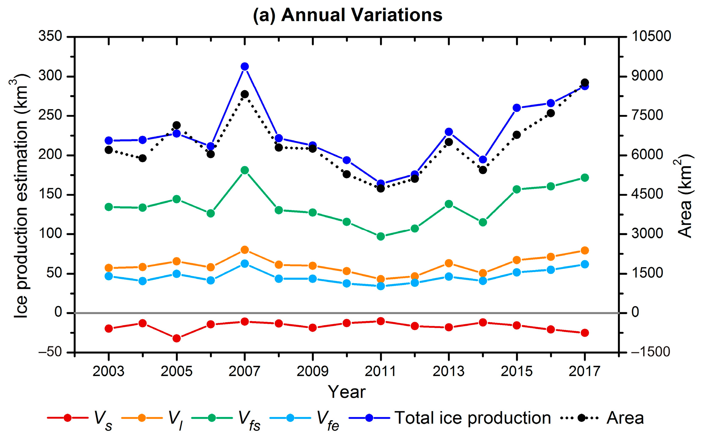
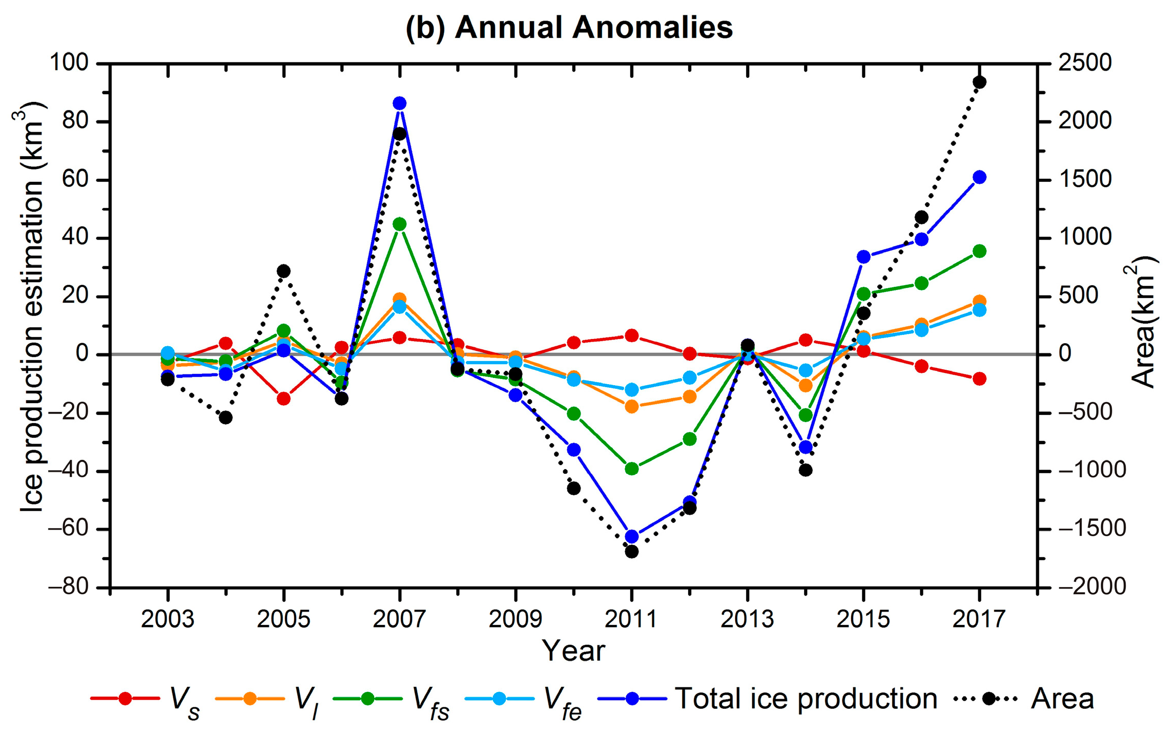
The interannual variation of RISP ice production is shown in Figure 2a, indicated by a dark blue line. Annual ice production during 2003–2017 exhibited substantial fluctuation between 164 and 313 km³. A linear regression model showed a slightly rising but not significant trend (R² = 0.0332, p = 0.516). The maximum ice production occurred in 2007. The annual RISP area is indicated by the black dotted line. According to a linear regression, it was strongly correlated to annual ice production (R² = 0.905, p = 0.000). The largest deviation to the fitting line occurred in 2005, when the area showed a peak while the ice production was relatively low. The anomaly plot of annual ice production and area confirms this result (Figure 2b). The area of 2005 showed a positive anomaly, while the ice production in that year showed only a weak positive anomaly.

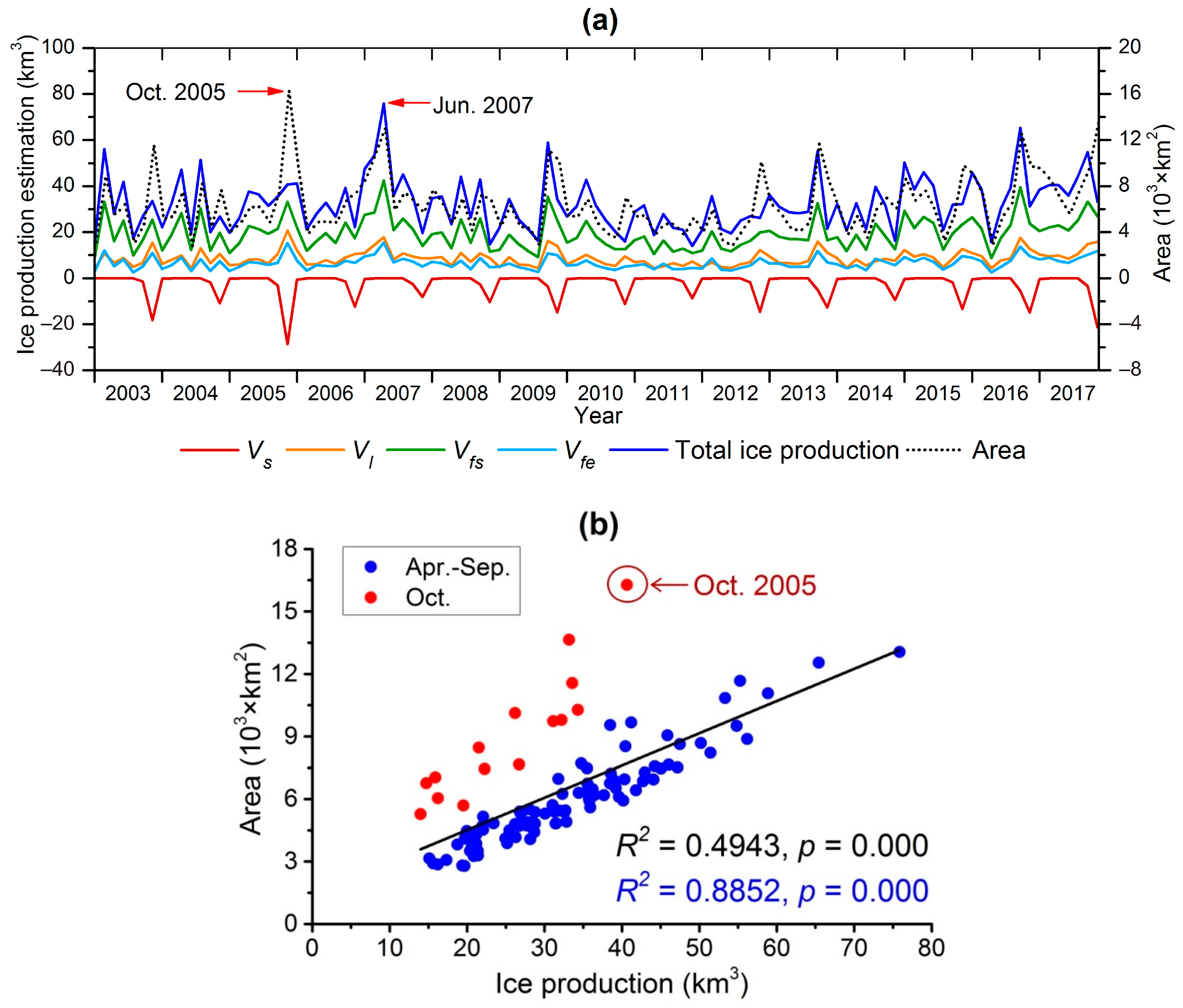
The monthly ice production and polynya area time series from April to October are plotted in Figure 3a. The highest monthly ice production occurred in June 2007. It contributed to 24.3% of the ice production in 2007, and was the main reason why 2007 was the peak year. Figure 3b is a scatter plot of monthly ice production and area. A significant linear relation exists, with R² = 0.4943, p = 0.000. In October 2005, the largest deviation from the fitting line occurred. Correspondingly, the black dotted line in Figure 3a (polynya area) ascends sharply to the highest peak in October 2005, while the dark blue line (ice production) increases much less. Hence, ice production in October 2005 was mainly responsible for the inconsistency between area and ice production in 2005. The monthly polynya area of October 2005 was also the highest for the whole period of analysis.

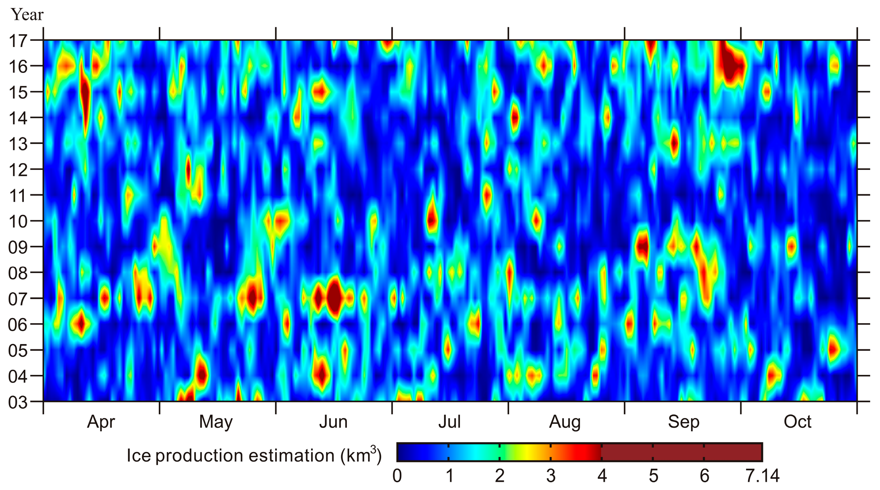
Figure 4 shows a Hovmöller diagram of daily RISP ice production. The X-axis represents dates, from 1 April to 31 October, whereas the Y-axis represents years, from 2003 to 2017. No obvious seasonal trend can be observed from this plot. Extreme high or low ice production events occurred occasionally and irregularly in every month.

This analysis shows that the RISP ice production reveals no clear annual or seasonal trend. Ice production is strongly correlated to polynya area, both in annual or monthly timescale. October 2005 and June 2007 are typical periods with extreme events. The highest polynya area and largest inconsistency between area and ice production occurred in October 2005, while the highest ice production occurred in June 2007.

3.2. Heat Flux Analysis

For the heat flux analysis, we divided the RISP ice production into four components according to their heat flux sources: the net solar radiation component V_s, the net longwave radiation component V_l, the sensible heat flux component V_fs, and the latent heat flux component V_fe. Figure 2 shows the variation and corresponding anomalies of V_s, V_l, V_fs, and V_fe as well as the total ice production and the polynya area. In Figure 2a, the total ice production is the sum of four components. It shows that V_fs accounts for 60.1% of total ice production, making the greatest contribution, followed by V_l (26.9%), V_fe (20.4%), and V_s (‒7.5%), making a negative contribution. V_l, V_fs, and V_fe show strong positive correlations with polynya area (R² = 0.9643, p = 0.000; R² = 0.9277, p = 0.000 and R² = 0.956, p = 0.000, respectively), while V_s is weakly correlated to polynya area (R² = 0.2503, p = 0.029). Figure 2b shows that V_l, V_fs, and V_fe have similar positive or negative anomalies with area and total ice production in years with evident anomalies, such as 2007, 2011, and 2017, while the anomaly of V_s follows a different pattern.

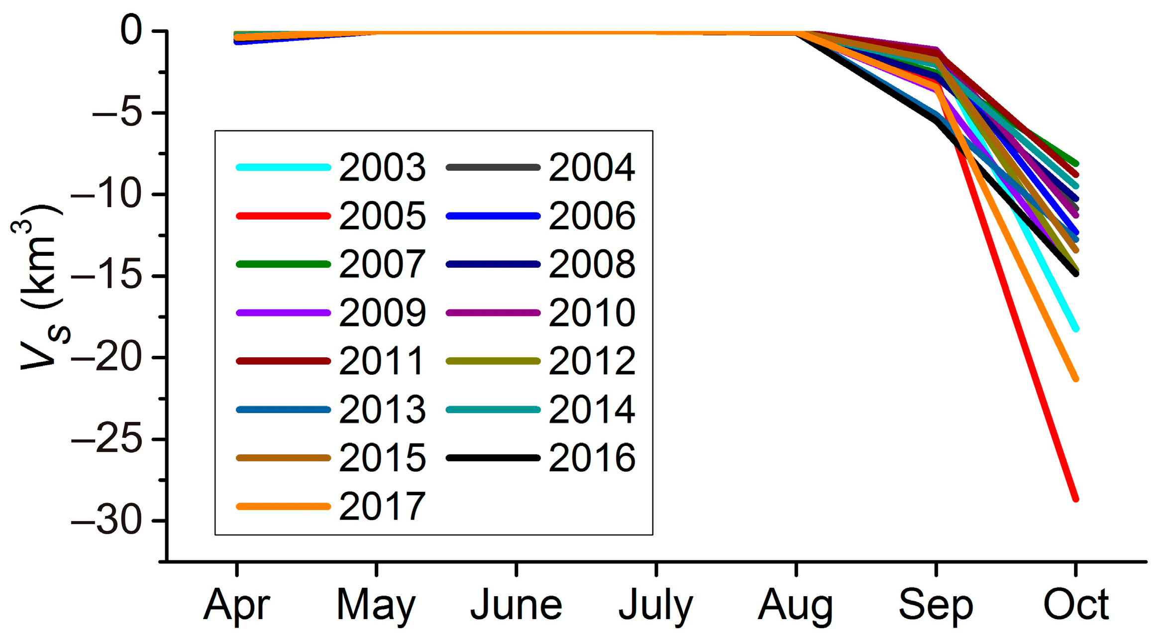
Figure 3a shows the monthly time series of V_s, V_l, V_fs, V_fe, total ice production, and polynya area. Like the annual time series, V_l, V_fs, and V_fe show strong positive relations with polynya area (R² = 0.9312, p = 0.000; R² = 0.6265, p = 0.000 and R² = 0.7492, p = 0.000, respectively), whereas V_s shows a cyclical pattern rather than a correlation with polynya area. Figure 5 shows that V_s is close to zero from April to August, and negative in September and October, making the greatest negative contribution to ice production in October. V_s, V_l, V_fs, and V_fe account for ‒1.5%, 24.5%, 58.0%, and 19.0% of total ice production between April and September, whereas in October, these proportions turn to ‒54.9%, 46.4%, 76.6%, and 31.9%, respectively. Note that the proportion of V_s increases 37-fold, caused by the drastically increased V_s in October.

The largest negative value of V_s occurred in October 2005, coinciding with the RISP area monthly maximum in October 2005. In October, V_s was strongly negatively correlated to the RISP area (R² = 0.9593, p = 0.000). Accordingly, this explains the inconsistency between ice production and polynya area in 2005, especially in October 2005: although the rapidly increasing RISP area in October 2005 enlarges V_l, V_fs, and V_fe, it also adds to the negative increasing of V_s. Therefore, the total ice production is balanced and only shows a mildly increasing trend instead of a sudden jump. The scatterplot in Figure 3b shows a significant linear relationship between monthly ice production and polynya area (R² = 0.4943, p = 0.000). Without the October data, the R² from April to September increases to 0.8852. Compared with the other data, the October data are more scattered and show relatively low ice production. Regarding the evidence in Figure 3a, the polynya area peaks in October of 2003, 2004, 2005, 2012, and 2017, but ice production only mildly increases or even decreases. This phenomenon did not occur from April to September because of the weak impact of solar radiation in the middle of winter. For example, the polynya area peaks in June 2007, September 2009, and September 2013 correspond to similar peaks in ice production with sharply increasing trends.

To summarize, V_fs makes the largest contribution to total ice production, followed by V_l and V_fe. These three components are strongly correlated with polynya area, whereas V_s makes a negative contribution, with an obvious seasonal trend. Its impact on ice production is weak from April to September, but it makes a negative contribution for October, strongly correlated to polynya area in October. As a result, in October, RISP ice production is reduced because of V_s, particularly the ice production in October 2005.

3.3. The Impact of Wind Forcing

Off-shore winds of katabatic nature are the predominant driving forces of the occurrence and maintaining of RISP [36,37,38]. We now examine the impact of wind forcing on ice production and its four components.

First, we estimated the time lag of wind forcing and compared six different types of wind speed. These are ECMWF wind speed (full speed and south‒north speed) averaged on the whole study area, ECMWF wind speed (full speed and south‒north speed) at the pixel with the highest ice production (near the edge of Ross Ice Shelf), AWS wind speed at Vito station, and Laurie II station. Each type of daily wind speed time series was linearly regressed on daily polynya area data, with a time lag of 0, 1, or 2 days. The results show that the wind speed of the previous day has the highest correlation with polynya area. Taking ECMWF full wind speed averaged on the whole study area as an example, we see that the R² with polynya area is equal to 0.0320 (p = 0.000) with no lag, 0.1128 (p = 0.000) with a one-day lag, and 0.0613 (p = 0.000) with a two-day lag, respectively. We next compared one-day-lag wind forcing with polynya area and ice production. The six types of wind speed have gaps if the AWS wind forcing data are missing or invalid. The results show that the polynya area has the strongest correlation with ECMWF full wind speed averaged over the whole study area (R² = 0.1465, p = 0.000), followed by the ECMWF south‒north wind speed averaged on the whole study area (R² = 0.1433, p = 0.000), and the wind speed at Vito station (R² = 0.1323, p = 0.000). The polynya area has a weak correlation with the ECMWF full wind speed at the pixel with the highest ice production, ECMWF south‒north wind speed at the pixel with highest ice production, and AWS wind speed at Laurie II station, with R² values equal to 0.0942 (p = 0.000), 0.0861 (p = 0.000), and 0.0109 (p = 0.192), respectively. To conclude, ECMWF full wind speed averaged over the whole study area has the highest correlation with polynya area, and its impact on polynya area has a time lag of approximately one day.

Based on the above analysis, the time series of ECMWF wind speed averaged on the whole study area with one day lag was linearly regressed on total ice production, V_s, V_l, V_fs, V_fe, and polynya area during 2003–2017. It showed R² values equal to 0.2026, 0.0006, 0.0861, 0.1984, 0.2159, and 0.1128, respectively. Wind speed explains at most 20.26% of the ice production variation. Wind speed has a stronger correlation with V_fs and V_fe than with V_s, V_l, and polynya area.

3.4. Extreme Wind Forcing Events

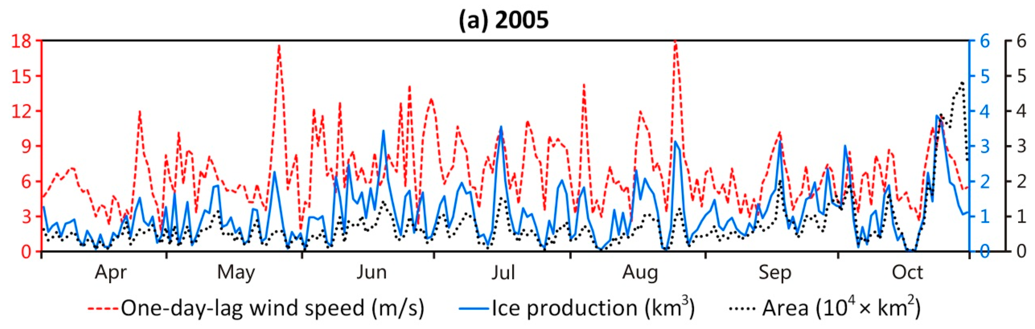
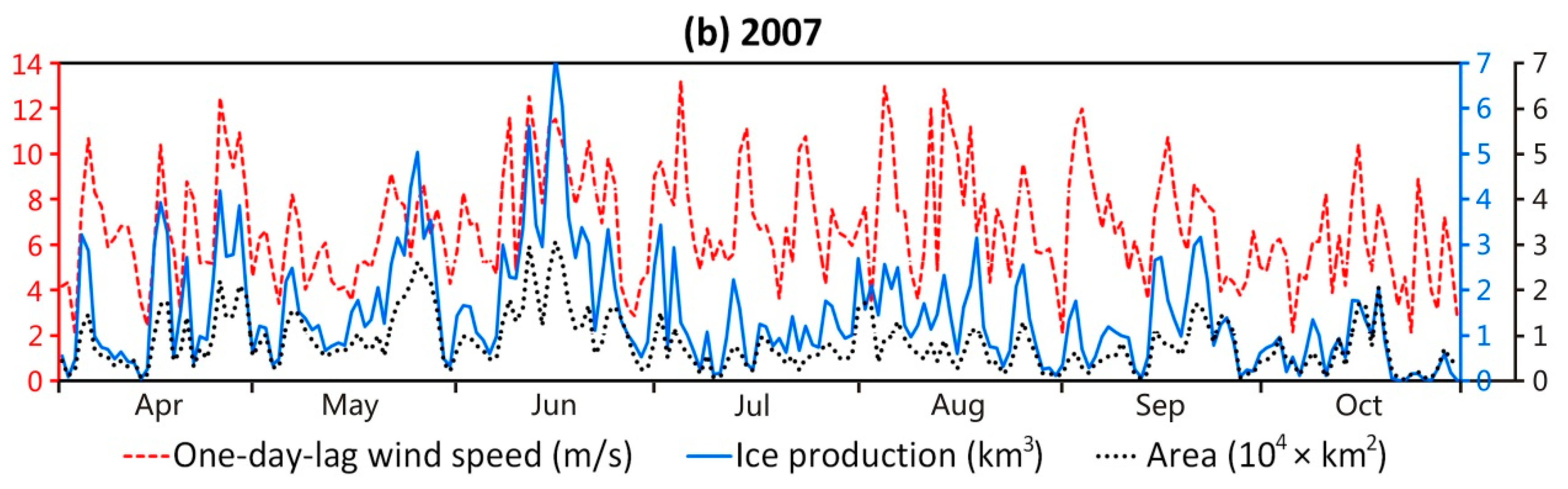
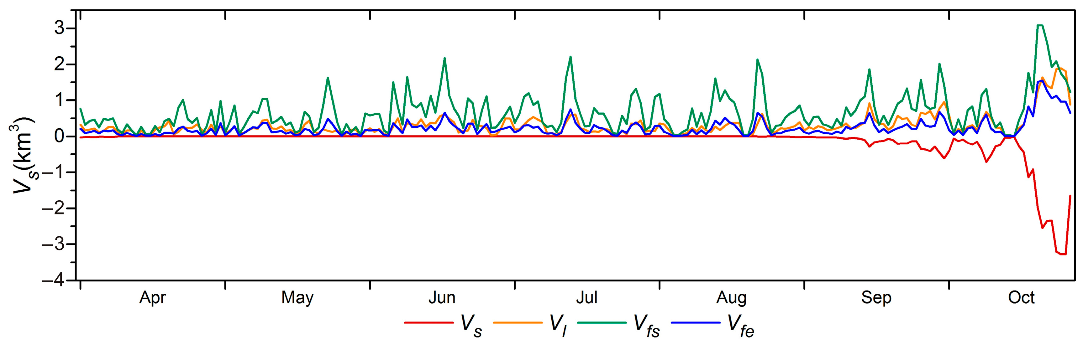
To further explore the two extreme events in October 2005 (maximum polynya area) and June 2007 (maximum ice production), Figure 6 plots the daily time series of one-day-lag wind speed, ice production, and polynya area in 2005 and 2007. By visual inspection, 68% of the peaks and valleys of one-day-lag wind speed and ice production coincide, and the correlations between them are weak but significant (R² = 0.2137, p = 0.000 for 2005; and R² = 0.2979, p = 0.000 for 2007). For October 2005, the peaks and valleys of wind speed and ice production coincide well, which means that the impact of wind speed on ice production is present. Polynya area abruptly increases to an extreme value at the end of October, while wind speed and ice production sharply decrease, leading to an inconsistency between area and ice production. This most likely is the main reason why monthly area and ice production are inconsistent in October 2005 in Figure 3. Figure 7 plots the time series of daily V_s, V_l, V_fs, and V_fe in 2005. Comparing Figure 6a with Figure 7, we see that at the end of October 2005, V_l showed similar peaks with polynya area, V_fs and V_fe decreased similarly to wind speed, and V_s decreased more strongly, showing a variation opposite to that of polynya area. The total ice production is evidently reduced by V_s. The R² values between wind speed and total ice production, V_s, V_l, V_fs, and V_fe and area in October 2005 were 0.4273, 0.2151, 0.2549, 0.4387, 0.4275, and 0.2411, respectively. Wind speed influences total ice production mainly via V_fs and V_fe, similar to the results over the whole time span. In June 2007, the variations of wind speed, area, and ice production largely coincided. Continuous high wind events kept the area and ice production at a high level. The R² values between wind speed and total ice production, V_s, V_l, V_fs, V_fe, and area in June 2007 were 0.6428, 0, 0.6473, 0.612, 0.6103, and 0.6593, respectively. Note that solar radiation is absent in June. The impacts of wind speed on V_l, V_fs, and V_fe are all strengthened as compared to October 2005. This is because wind speed has a stronger impact on area, and V_l, V_fs, and V_fe are all directly proportional to area (Equations (1) and (7)).

We next use a series of images to monitor the spatial dynamic of RISP. Figure 8 presents the extreme wind events on 19–28 October 2005 and 13–22 June 2007. Each of the vector plots of wind forcing on the top compares the ice production distributions of the next day on the bottom. During 19–28 Oct 2005, the R² value between wind speed and ice production of the next day equals 0.5256 (p = 0.019), and during 13–22 June 2007, it equals 0.6325 (p = 0.006). Many aspects of the wind events can be clearly observed from this series of images, particularly that the RISP area is enlarged and ice production increases under strong wind events, whereas it decreases when wind forcing is weak. The large RISP area in these two periods is the result of persistent strong offshore winds. However, the ice production rate in October 2005 was generally lower than in June 2007.

The shape of the RISP area is to some degree correlated to the wind force. During the period of 26–28 October 2005, for example, the prevailing wind was southwestern. As a result, the distribution of RISP moved to the east, whereas during the period of 18–20 June 2007, a strong southern wind event between 170°E and 180°E longitude resulted in a northward area extension at the same location.

4. Discussion

By using heat flux sources analysis, we estimated that sensible heat flux V_fs accounted for 60.1% of the total ice production, followed by longwave radiation V_l accounting for 26.9% and latent heat flux V_fe accounting for 20.4%, and solar radiation V_s accounted for −7.5%. Woert [25] quantified three heat flux components on the ocean‒atmosphere interface of the Terra Nova Bay polynya, a smaller polynya also in the Ross Sea, during winter 1988–1990. On an average, sensible heat flux, longwave heat flux and latent heat flux accounted for 67.0%, 11.3%, and 21.7%, respectively. Comparing with our study, the sensible heat flux and the latent heat flux account for similar proportions, but the longwave radiation occupies a much smaller proportion. Woert budgeted the heat fluxes under the assumption that the cloud cover fraction was constantly equal to 50%, followed by a longwave flux sensitivity analysis. Changing cloud cover from 0 to 100% gave an uncertainty to longwave heat flux up to 50%. The result suggested that cloud fraction contributed to a large uncertainty in the longwave radiation budget. In our study, the variation of cloud cover is involved in the calculation of incoming longwave radiation, an input variable provided by the reanalysis data. We inferred that the assumed constant 50% cloud fraction was mainly responsible for the different proportions of the longwave heat flux. Haid and Timmermann [27] simulated heat flux on three coastal polynyas in the southwestern Weddell Sea during May–September 1990–2009. The average sensible heat flux, longwave radiation, latent heat flux, and solar radiation accounted for 61.3%, 24.1%, 16.1%, and ‒1.5%, respectively, but their study period excluded October, when solar radiation contributes more. Therefore, our study shows a stronger negative contribution of solar radiation.

The seasonal variation of solar radiation in Figure 5 is mainly related to polar night and polar day. Since our study area is located at a high latitude, near 77°S, both the polar night and polar day last for a long time. The polar night starts around 27 April and ends around 18 August, whereas the polar day starts around 27 October and ends around 15 February. It shifts from no solar illumination to high solar illumination in less than two months. Since the solar radiation component V_s is proportional to the polynya area (Equations (1) and (7)) and the polynya area is correlated to extreme wind events, or strong wind events that lead to different effects to V_s and total ice production in different seasons. A strong wind event during the polar night has no influence on V_s, and leads to an increasing polynya area, V_l, V_fs, and V_fe and, thus, to increased total ice production. A strong wind event during polar day, however, leads to a strongly negative V_s. Such a total increasing ice production usually partly balances. As Figure 7 shows, V_s decreased sharply at the end of October 2005, coinciding with the start of the polar day. We conclude that solar radiation condition has an evident impact on sea ice production.

Six different kinds of wind speed were regressed with polynya area. During most of the study period, the ECMWF full wind speed averaged over the study area had the highest correlation with polynya area. The results show that wind speed measured at the Vito station was more highly correlated than that measured at the Laurie II station. Wind speed averaged over the study area was more highly correlated than wind speed measured at a single station. Therefore, we chose ECMWF full wind speed averaged over the study area as the model input for estimating ice production.

Wind forcing influences polynya ice production via two main mechanisms. First, strong wind events lead to an increasing polynya area. In the estimation of heat flux components, all four components are directly proportional to the polynya area (Equations (1) and (7)). Consequently, strong wind events lead to increasing ice production. As our results show, polynya area has the highest correlation with the wind speed of the previous day. Dale et al. reported similar findings, i.e., the strongest negative correlation between ice concentration and wind speed occurred after a 12-h time lag [38]. Second, high wind speed accelerates heat exchange and the phase transformation of ice. This impact is related to V_fs and V_fe, both being directly proportional to wind speed but not to V_s and V_l. Apparently, such impact has no time lag. According to the linear regression between wind speed and ice production components during the full time series and extreme periods, wind speed influences total ice production via the two main components, V_fs and V_fe. Since wind speed has a much stronger correlation with V_fs and V_fe than with polynya area, wind forcing influences V_fs and V_fe not only through the first mechanism mentioned above, but also through the second one, as wind speed of the previous day is correlated to wind speed on the day itself. However, V_s and V_l are only influenced by the first mechanism. In October 2005, both mechanisms were evident, similar to during the full time series. In June 2007, however, the first mechanism’s impact on polynya area was obviously strengthened. To summarize, both kinds of wind forcing impacts are present, but in different polynya events, they show different degrees of importance.

In 2005 and 2007, 68% of the peaks and valleys of ice production variation coincided with those in the one-day-lag wind speed time series. Bromwich et al. [36] examined the open water fraction and atmospheric forcing on RISP in winter from 1988 to 1991. They found that approximately 60% of the polynya events were linked to katabatic surge events, which was consistent with our results. According to a linear regression between one-day-lag wind speed and ice production over the whole study period, wind speed can explain approximately 20% of the ice production variation (Figure 6). During a specific extreme event, wind speed can explain approximately 50% of the ice production variation. The variation in polynya ice production is a synergistic result of various environment impacts with dynamic and thermodynamic processes, including atmospheric forcing, oceanic currents, air and water temperature, air humidity, ocean salinity, and iceberg drift. New data with finer resolution or a more specific spatial analysis are needed for further study of the ice production variation.

5. Conclusions

In this study, we divided the ice production of RISP into four components according to heat flux sources. The sensible heat flux component V_fs accounted for 60.1% of the total ice production, the longwave radiation component V_l for 26.9%, the latent heat flux component V_fe for 20.4%, the solar radiation component V_s for ‒7.5% which decreased to ‒54.9% in October. V_l, V_fs, and V_fe highly correlate with the RISP area size, whereas V_s negatively correlates with the RISP area size in October, and has a weak influence from April to September.

ECMWF wind speed averaged over the whole study area was highly correlated with polynya area. Approximately 68% of the peaks and valleys of the wind speed time series coincided with ice production time series, and 20% of the RISP ice production variation could be explained by wind speed. Wind forcing showed different impacts on ice production during different seasons. Since ice production is strongly correlated to polynya area, and polynya area has a significant correlation with wind speed, a strong wind event in April–September will lead to increasing polynya area, along with increasing ice production. A strong wind event in October followed by sharp area expansion, however, may only lead to slightly increasing or even decreasing ice production, due to a strong negative contribution of V_s. In particular, October 2005 showed a large inconsistency between polynya area and ice production.

Wind forcing influences V_fs and V_fe by having an impact on polynya area, and on the heat exchange and phase transformation of ice. Wind forcing influences V_s and V_l only by impact on the polynya area. The two mechanisms have an evident impact on ice production but show different degrees of importance during different extreme periods. The expansion and spatial distribution of RISP are correlated to the wind speed and direction. Persistent offshore winds were found to be responsible for large polynya area and high ice production in October 2005 and June 2007.

References

- Smith, S.D.; Muench, R.D.; Pease, C.H. Polynyas and leads: An overview of physical processes and environment. J. Geophys. Res. 1990, 95, 9461–9479. [Google Scholar] [CrossRef]
- Lemke, P. Open windows to the polar oceans. Science 2001, 292, 1670–1671. [Google Scholar] [CrossRef] [PubMed]
- Maqueda, M.M.; Willmott, A.J.; Biggs, N.R. Polynya dynamics: A review of observations and modeling. Rev. Geophys. 2004, 42. [Google Scholar] [CrossRef]
- Tamura, T.; Ohshima, K.I.; Nihashi, S. Mapping of sea ice production for Antarctic coastal polynyas. Geophys. Res. Lett. 2008, 35, L07606. [Google Scholar] [CrossRef]
- Kern, S. Wintertime Antarctic coastal polynya area: 1992–2008. Geophys. Res. Lett. 2009, 36, L14501. [Google Scholar] [CrossRef]
- Gordon, A.L.; Comiso, J.C. Polynyas in the southern ocean. Sci. Am. 1988, 258, 90–97. [Google Scholar] [CrossRef]
- Jacobs, S.S.; Comiso, J.C. Sea ice and oceanic processes on the Ross Sea continental shelf. J. Geophys. Res. Oceans 1989, 94, 18195–18211. [Google Scholar] [CrossRef]
- Pease, C.H. The size of wind-driven coastal polynyas. J. Geophys. Res. 1987, 92, 7049–7059. [Google Scholar] [CrossRef]
- Martin, S.; Polyakov, I.; Markus, T.; Drucker, R. Okhotsk Sea Kashevarov Bank polynya: Its dependence on diurnal and fortnightly tides and its initial formation. J. Geophys. Res. Oceans 2004, 109. [Google Scholar] [CrossRef] [Green Version]
- Martin, S.; Drucker, R.S.; Kwok, R. The areas and ice production of the western and central Ross Sea polynyas, 1992–2002, and their relation to the B-15 and C-19 iceberg events of 2000 and 2002. J. Mar. Syst. 2007, 68, 201–214. [Google Scholar] [CrossRef]
- Nihashi, S.; Ohshima, K.I. Circumpolar mapping of Antarctic coastal polynyas and landfast sea ice: Relationship and variability. J. Clim. 2015, 28, 3650–3670. [Google Scholar] [CrossRef]
- Kwok, R. Ross Sea ice motion, area flux, and deformation. J. Clim. 2005, 18, 3759–3776. [Google Scholar] [CrossRef]
- Drucker, R.; Martin, S.; Kwok, R. Sea ice production and export from coastal polynyas in the Weddell and Ross Seas. Geophys. Res. Lett. 2011, 38, L17502. [Google Scholar] [CrossRef]
- Comiso, J.C.; Kwok, R.; Martin, S.; Gordon, A.L. Variability and trends in sea ice extent and ice production in the Ross Sea. J. Geophys. Res. 2011, 116, C04021. [Google Scholar] [CrossRef]
- Drucker, R.; Martin, S.; Moritz, R. Observations of ice thickness and frazil ice in the St. Lawrence Island polynya from satellite imagery, upward looking sonar, and salinity/temperature moorings. J. Geophys. Res. Oceans 2003, 108. [Google Scholar] [CrossRef] [Green Version]
- Willmes, S.; Adams, S.; Schröder, D.; Heinemann, G. Spatio-temporal variability of polynya dynamics and ice production in the Laptev Sea between the winters of 1979/80 and 2007/08. Polar Res. 2011, 30, 5971. [Google Scholar] [CrossRef] [Green Version]
- Cheng, Z.; Pang, X.; Zhao, X.; Tan, C. Spatio-Temporal Variability and Model Parameter Sensitivity Analysis of Ice Production in Ross Ice Shelf Polynya from 2003 to 2015. Remote Sens. 2017, 9, 934. [Google Scholar] [CrossRef]
- Ebner, L.; Schröder, D.; Heinemann, G. Impact of Laptev Sea flaw polynyas on the atmospheric boundary layer and ice production using idealized mesoscale simulations. Polar Res. 2011, 30, 7210. [Google Scholar] [CrossRef] [Green Version]
- Bauer, M.; Schröder, D.; Heinemann, G.; Willmes, S.; Ebner, L. Quantifying polynya ice production in the Laptev Sea with the COSMO model. Polar Res. 2013, 32, 55–61. [Google Scholar] [CrossRef]
- Preußer, A.; Willmes, S.; Heinemann, G.; Paul, S. Thin-ice dynamics and ice production in the Storfjorden polynya for winter-seasons 2002/2003–2013/2014 using MODIS thermal infrared imagery. Cryosphere 2015, 9, 1063–1073. [Google Scholar] [CrossRef]
- Tamura, T.; Ohshima, K.I.; Fraser, A.D.; Williams, G.D. Sea ice production variability in Antarctic coastal polynyas. J. Geophys. Res. 2016, 121, 2967–2979. [Google Scholar] [CrossRef]
- Parmiggiani, F. Fluctuations of Terra Nova Bay polynya as observed by active (ASAR) and passive (AMSR-E) microwave radiometers. Int. J. Remote Sens. 2006, 27, 2459–2467. [Google Scholar] [CrossRef]
- Adams, S.; Willmes, S.; Heinemann, G.; Rozman, P.; Timmermann, R.; Schroeder, D. Evaluation of simulated sea-ice concentrations from sea-ice/ocean models using satellite data and polynya classification methods. Polar Res. 2011, 30. [Google Scholar] [CrossRef]
- Markus, T.; Burns, B.A. A method to estimate subpixel-scale coastal polynyas with satellite passive microwave data. J. Geophys. Res. 1995, 100, 4473–4487. [Google Scholar] [CrossRef]
- Van Woert, M.L. Wintertime dynamics of the Terra Nova Bay polynya. J. Geophys. Res. Oceans 1999, 104, 7753–7769. [Google Scholar] [CrossRef] [Green Version]
- Ohshima, K.I.; Watanabe, T.; Nihashi, S. Surface heat budget of the Sea of Okhotsk during 1987–2001 and the role of sea ice on it. J. Meteorol. Soc. Jpn. 2003, 81, 653–677. [Google Scholar] [CrossRef]
- Haid, V.; Timmermann, R. Simulated heat flux and sea ice production at coastal polynyas in the southwestern Weddell Sea. J. Geophys. Res. 2013, 118, 2640–2652. [Google Scholar] [CrossRef] [Green Version]
- Nakata, K.; Ohshima, K.I.; Nihashi, S.; Kimura, N.; Tamura, T. Variability and ice production budget in the Ross Ice Shelf Polynya based on a simplified polynya model and satellite observations. J. Geophys. Res. 2015, 120, 6234–6252. [Google Scholar] [CrossRef] [Green Version]
- Massom, R.A.; Harris, P.T.; Michael, K.J.; Potter, M.J. The distribution and formative processes of latent-heat polynyas in East Antarctica. Ann. Glaciol. 1998, 27, 420–426. [Google Scholar] [CrossRef]
- Dee, D.P.; Uppala, S.M.; Simmons, A.J.; Berrisford, P.; Poli, P.; Kobayashi, S.; Andrae, U.; Balmaseda, M.A.; Balsamo, G.; Bauer, P.; et al. The ERA-Interim reanalysis: Configuration and performance of the data assimilation system. Q. J. R. Meteorol. Soc. 2011, 137, 553–597. [Google Scholar] [CrossRef]
- Lazzara, M.A.; Weidner, G.A.; Keller, L.M.; Thom, J.E.; Cassano, J.J. Antarctic Automatic Weather Station Program: 30 Years of Polar Observation. Bull. Am. Meteorol. Soc. 2012, 93, 1519–1537. [Google Scholar] [CrossRef]
- Spreen, G.; Kaleschke, L.; Heygster, G. Sea ice remote sensing using AMSR-E 89 GHz channels. J. Geophys. Res. 2008, 113. [Google Scholar] [CrossRef]
- Beitsch, A.; Kaleschke, L.; Kern, S. Investigating high-resolution AMSR2 sea ice concentrations during the February 2013 fracture event in the Beaufort Sea. Remote Sens. 2014, 6, 3841–3856. [Google Scholar] [CrossRef]
- Kern, S.; Spreen, G.; Kaleschke, L.; de La Rosa, S.; Heygster, G. Polynya Signature Simulation Method polynya area in comparison to AMSR-E 89 GHz sea-ice concentrations in the Ross Sea and off the Adélie Coast, Antarctica, for 2002–05: First results. Ann. Glaciol. 2007, 46, 409–418. [Google Scholar] [CrossRef]
- AMSR-E/Aqua Daily L3 6.25 km 89 GHz Brightness Temperature Polar Grids, Version 3. Available online: http://nsidc.org/data/ae_si6/ (accessed on 26 June 2018).
- Bromwich, D.; Liu, Z.; Rogers, A.N.; Van Woert, M.L. Winter atmospheric forcing of the Ross Sea polynya. Ocean Ice Atmos. Interact. Antarct. Cont. Margin 1998, 75, 101–133. [Google Scholar]
- Holland, P.R.; Kwok, R. Wind-driven trends in Antarctic sea-ice drift. Nat. Geosci. 2012, 5, 872. [Google Scholar] [CrossRef]
- Dale, E.R.; McDonald, A.J.; Coggins, J.H.J.; Rack, W. Atmospheric forcing of sea ice anomalies in the Ross Sea polynya region. Cryosphere 2017, 11, 267. [Google Scholar] [CrossRef]
Figure 1.
(a) Location map of the study area. The red rectangle indicates the location of (b). (b) Spatial distribution map of the Ross Ice Shelf Polynya (RISP) occurrence frequency. The study area is enclosed by the white line. Two Automatic Weather Stations are marked by red points.
Figure 2.
Annual variations (a) and anomalies (b) of polynya area, ice production and its four components, Vs, VI, Vfs and Vfe. Annual polynya area is the average daily area from April to October. Annual ice production is the sum of daily ice production from April to October, similar for Vs, VI, Vfs, Vfe. The annual anomalies in (b) equal values in (a) minus the 15-year averaged values.
Figure 3.
(a) Time series of monthly polynya area, ice production and its four components, Vs, VI, Vfs and Vfe from 2003 to 2017, restricted to April to October. (b) Linear regression between monthly polynya area and ice production. Blue points refer to April to September data, and red points to October data. R2, p-value and fitting line in black refer to all points, and values in blue refer to the blue points.
Figure 4.
Hovmöller diagram of daily RISP sea ice production between 2003 and 2017, from April to October. The X-axis indicates the month and date; the Y-axis indicates the year.
Figure 5.
Seasonal variation of Vs. The largest negative value occurred in October 2005.
Figure 6.
Time series of daily wind speed with one day lag, ice production and polynya area in 2005 (a) and 2007 (b).
Figure 7.
Time series of daily Vs, Vl, Vfs, and Vfe in 2005.
Figure 8.
Comparison of wind forcing vector plots and ice production maps of the next day. In the wind forcing vector plots, the background color from yellow to red indicates wind speed from low to high. The arrows mark the wind direction, and the length of the arrows indicates wind speed. The ice production maps show the area of RISP where the color, from grey to black, indicates the ice production rate. Two extreme wind events lasting 10 days are shown in October 2005 (a) and June 2007 (b). At some dates the polynya area extends beyond the study area, which encloses the area with a polynya occurrence frequency >10% and excludes open water.
© 2019 by the authors. Licensee MDPI, Basel, Switzerland. This article is an open access article distributed under the terms and conditions of the Creative Commons Attribution (CC BY) license (http://creativecommons.org/licenses/by/4.0/).
Share and Cite
MDPI and ACS Style
Cheng, Z.; Pang, X.; Zhao, X.; Stein, A. Heat Flux Sources Analysis to the Ross Ice Shelf Polynya Ice Production Time Series and the Impact of Wind Forcing. Remote Sens. 2019, 11, 188. https://doi.org/10.3390/rs11020188
AMA Style
Cheng Z, Pang X, Zhao X, Stein A. Heat Flux Sources Analysis to the Ross Ice Shelf Polynya Ice Production Time Series and the Impact of Wind Forcing. Remote Sensing. 2019; 11(2):188. https://doi.org/10.3390/rs11020188
Chicago/Turabian StyleCheng, Zian, Xiaoping Pang, Xi Zhao, and Alfred Stein. 2019. "Heat Flux Sources Analysis to the Ross Ice Shelf Polynya Ice Production Time Series and the Impact of Wind Forcing" Remote Sensing 11, no. 2: 188. https://doi.org/10.3390/rs11020188
Note that from the first issue of 2016, this journal uses article numbers instead of page numbers. See further details here.