Mapping and Monitoring Rice Agriculture with Multisensor Temporal Mixture Models


Lamont-Doherty Earth Observatory, Columbia University, Palisades, NY 10964, USA
*
Author to whom correspondence should be addressed.
Remote Sens. 2019, 11(2), 181; https://doi.org/10.3390/rs11020181
Submission received: 17 December 2018
/
Revised: 11 January 2019
/
Accepted: 16 January 2019
/
Published: 18 January 2019
(This article belongs to the Special Issue Applications of Land Surface Temperature and its Combination with other Satellite Land Products)
Abstract
:Rice is the staple food for more than half of humanity. Accurate prediction of rice harvests is therefore of considerable global importance for food security and economic stability, especially in the developing world. Landsat sensors have collected coincident thermal and optical images for the past 35+ years, and so can provide both retrospective and near-realtime constraints on the spatial extent of rice planting and the timing of rice phenology. Thermal and optical imaging capture different physical processes, and so provide different types of information for phenologic mapping. Most analyses use only one or the other data source, omitting potentially useful information. We present a novel approach to the mapping and monitoring of rice agriculture which leverages both optical and thermal measurements. The approach relies on Temporal Mixture Models (TMMs) derived from parallel Empirical Orthogonal Function (EOF) analyses of Landsat image time series. Analysis of each image time series is performed in two stages: (1) spatiotemporal characterization, and (2) temporal mixture modeling. Characterization evaluates the covariance structure of the data, culminating in the selection of temporal endmembers (EMs) representing the most distinct phenological cycles of either vegetation abundance or surface temperature. Modeling uses these EMs as the basis for linear TMMs which map the spatial distribution of each EM phenological pattern across study area. The two metrics we analyze in parallel are (1) fractional vegetation abundance (Fv) derived from spectral mixture analysis (SMA) of optical reflectance, and (2) land surface temperature (LST) derived from brightness temperature (Tb). These metrics are chosen on the basis of being straightforward to compute for any (cloud-free) Landsat 4-8 image in the global archive. We demonstrate the method using a 90 × 120 km area in the Sacramento Valley of California. Satellite Tb retrievals are corrected to LST using a standardized atmospheric correction approach and pixelwise fractional emissivity estimates derived from SMA. LST and Tb time series are compared to field station data in 2016 and 2017. Uncorrected Tb is observed to agree with the upper bound of the envelope of air temperature observations to within 3 °C on average. As expected, LST estimates are 3 to 5 °C higher. Soil T, air T, Tb and LST estimates can all be represented as linear transformations of the same seasonal cycle. The 3D temporal feature spaces of Fv and LST clearly resolve 5 and 7 temporal EM phenologies, respectively, with strong clustering distinguishing rice from other vegetation. Results from parallel EOF analyses of coincident Fv and LST image time series over the 2016 and 2017 growing seasons suggest that TMMs based on single year Fv datasets can provide accurate maps of crop timing, while TMMs based on dual year LST datasets can provide comparable maps of year-to-year crop conversion. We also test a partial-year model midway through the 2018 growing season to illustrate a potential real-time monitoring application. Field validation confirms the monitoring model provides an upper bound estimate of spatial extent and relative timing of the rice crop accurate to 89%, even with an unusually sparse set of usable Landsat images.
1. Introduction
Rice agriculture is critical for global food security. Much of the developing world relies on rice production for subsistence and/or commercial purposes. Rice is the largest food source for the world’s poor, and more than half of the world’s population relies on rice as its staple food [1]. In terms of nutrition, rice provides 21% of global human per capita energy and 15% of per capita protein. More land area is used for rice production than any other agricultural crop [2]. Predictability of global and regional rice production has obvious and significant implications for the management of both human and natural systems. For these predictions to be accurate, yield models must be provided with inputs of abundant, accurate observations in order to constrain fundamental variables such as planted area and timing of key phenological transitions (e.g., [3]). Similar biogeophysical observations can also address concerns important to commercial growers like optimization of the use of water [4] and nutrient additives [5]; assessment of extent and severity of weeds [6], pests [7], and diseases [8]; and independent verification of alternative cropping practices [9].
One cost effective tool to provide these observations is the spatiotemporal analysis of satellite imagery. Free global decameter (10 to 100 m) resolution multispectral optical and thermal imagery already exists through the Landsat program, with data extending back to the early 1980s [10]. The Landsat program has been supplemented since 2015 by the addition of the optical-only Sentinel-2 constellation [11]. Additional hectometer (100 to 1000 m) resolution imagery is available through the MODIS, VIIRS, and Sentinel-3 programs. The global archive of meter to hectometer resolution optical satellite imagery is expected to continue to grow into the future as further missions are planned in both the public and private sectors. This rich set of observations—with global coverage—can facilitate both retrospective and prospective analyses for a wide range of agricultural applications.
Rigorous characterization of plant life cycles and cropping practices is required in order to confidently relate satellite measurements to crop conditions. In recent decades, significant effort has been devoted—and much success has been achieved—in studying and improving rice agriculture around the world [12]. As a result, rice is one of the best-understood crops on Earth from an agronomic perspective. Despite this progress, significantly less work has been done to characterize how the biogeophysical progression of the land surface characteristic of rice agriculture is recorded by optical and thermal satellite imagery. To date, most applications of satellite imagery for rice agriculture have focused on discrete classification and mapping of rice extent (e.g., [13,14,15,16,17]), rather than on a physical understanding of how the land surface properties and processes that characterize the phenological cycle of rice crops are manifest in satellite observations. This physically-based strategy is the approach taken in this study.
An obvious distinction between rice and most other crops is that rice is often (but not always) grown in paddies. In paddy rice, this fundamental difference results in substantial evaporative cooling and near-complete absorption in optical infrared wavelengths early in the cropping cycle, neither of which are generally present for non-rice crops in the same landscape. Imaging by satellites at both optical VSWIR (Visible through Shortwave Infrared, 0.4–2.5 µm) and TIR (Thermal Infrared, 8–14 µm) wavelengths results in both (1) lower TIR temperature measurements, and (2) lower overall VSWIR albedo relative to non-rice crops. Because the biogeophysical signal manifests in both VSWIR and TIR wavelength regimes, the evolution of the rice crop throughout a growing season occupies a more unique trajectory in the combined geophysical parameter space comprised of both VSWIR and TIR than in the space of either parameter alone. This provides an opportunity to improve the accuracy of crop-specific maps of rice based on optical imagery alone by supplementing with thermal image time series, illustrating the added value of the thermal satellite sensors and the importance of continuity in intercalibrated satellite thermal image collection.
This analysis presents a straightforward, physically-based approach for the mapping and monitoring of rice agriculture. Using the Sacramento Valley of California as our example area, we apply the methodology of spatiotemporal characterization and modeling, first described in detail by [18], to the special case of a parallel analysis of the twin data streams from coincident Landsat 8 OLI (Operational Land Imager) and TIRS (Thermal Infrared Sensor) image time series. The resulting VSWIR and TIR data spaces each characterize complementary features of the biogeophysical evolution of the agricultural landscape. Using endmembers (EMs) that represent distinct temporal trajectories, independently derived from each data stream, we demonstrate the method by mapping both the timing and presence/absence of rice crops across 2 years. Finally, we also show the seasonal evolution of the landscape in Temperature vs. Vegetation (TV) space. This suggests more detailed investigation into the spatiotemporal analysis of evapotranspiration (ET) as an attractive avenue for future work, as also proposed by [19], to potentially directly address several of the outstanding research questions identified by the recent NRC Decadal Survey [20].
While a considerable body of literature exists on mapping rice from optical satellite imagery, to our knowledge, previous work has generally focused on applying a variety of complex statistical algorithms to VSWIR data, usually without using thermal information. Some previous studies have included thermal data into their algorithms, but rarely in a physically-based way. The approach presented here explicitly integrates multitemporal thermal and optical measurements to discriminate between distinct phenological cycles, resulting in an improved quantitative understanding of land surface processes and coincident energy fluxes. Additional benefits include relative mathematical simplicity and a direct grounding in biogeophysical processes.
1.1. Background—Study Area
1.1.1. Regional Thermal Setting
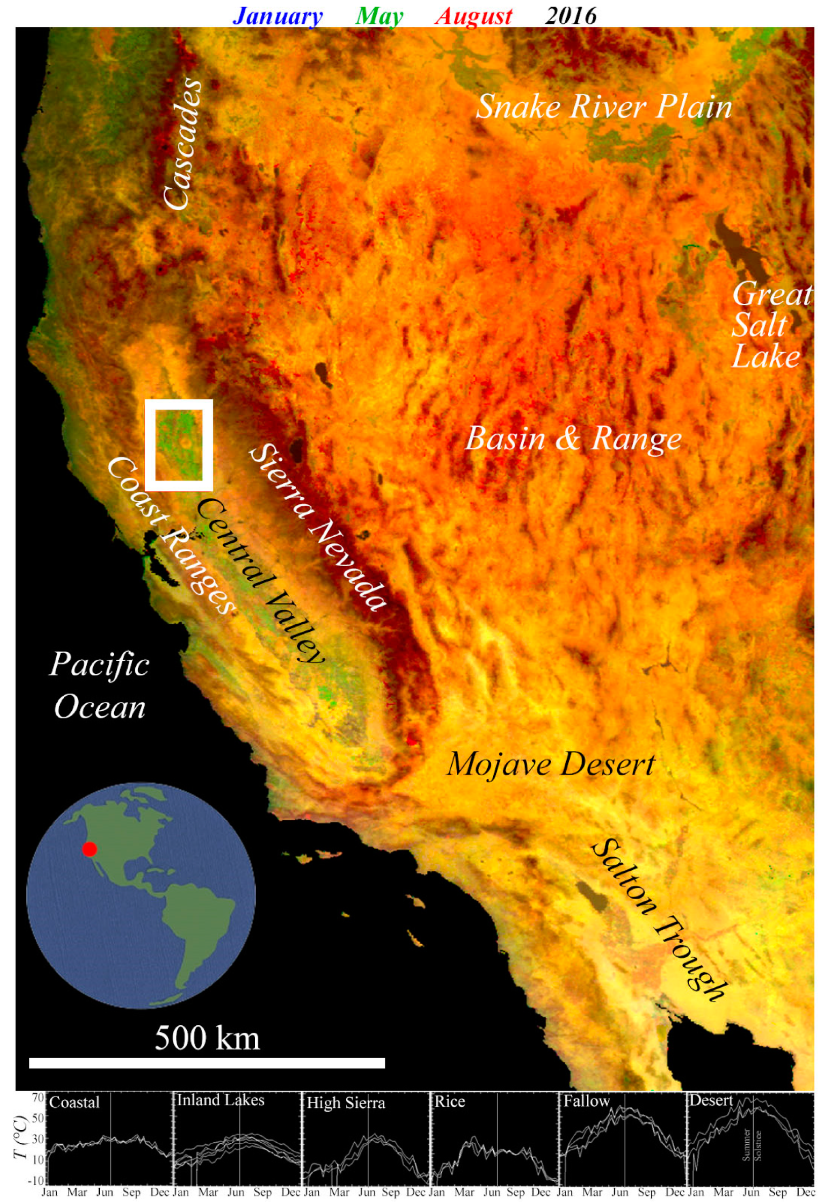
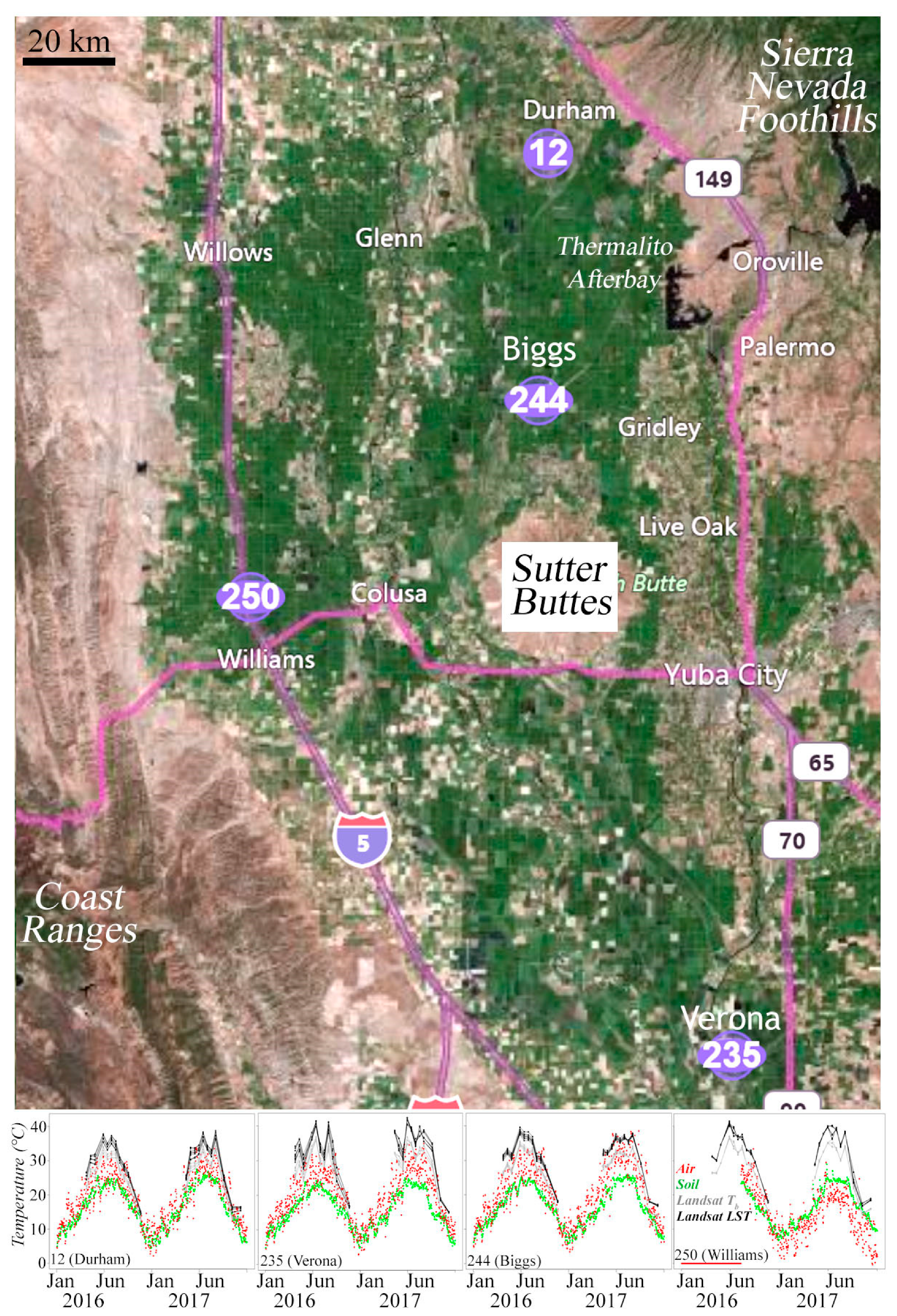
Figure 1 shows the study area in regional context using a tri-temporal thermal composite image. The northern portion of the Great Central Valley of California (area within and around the white box) is one of the most productive rice growing regions on Earth. Land use in the valley is dominated by intensive agricultural production of a wide range of commodity and specialty crops. The Sacramento Valley is characterized by Köppen Climate Csa (Hot Summer Mediterranean). The vast majority of precipitation is delivered between the late fall and the early spring, with summers being characterized by dry, hot days with sparse cloud cover. A wide range of soil types exist in California, sometimes distinguishable on the basis of VSWIR reflectance [21]. Clay-rich soils are common in the northern portion of the valley, providing a nearly ideal natural substrate to support the standing water commonly used in intensive rice agriculture. Water in the region is highly controlled through a network of government-run water projects. Effectively all summer agriculture in the Central Valley is irrigated using a combination of water captured by reservoirs located in the surrounding foothills and pumped from wells.
The colors on Figure 1 illustrate at a glance the typical thermal evolution of the region over the first half of the calendar year. In this figure, the blue, green, and red channels of the image represent land surface temperatures (LSTs) in January, May, and August of 2016, respectively. No locations are bright blue because the landscape is universally colder in January than in May or August. The Mojave Desert appears as yellow (red + green) because its temperature (bottom time series) generally mimics the annual cycle of solar insolation. In contrast, the Basin and Range takes longer to heat and maps with a more reddish hue. High elevations in the Sierra Nevada and Coast Ranges appear as dark red because seasonal snowpack results in low winter temperatures that then rapidly rise once the snowpack melts in late spring/early summer. Agriculture in the Central Valley and Snake River Plain appears green because surface temperature in the May image is generally elevated due to the low thermal inertia of bare, dry fields. Once crops have grown, however, the associated evapotranspiration (ET) significantly cools the landscape during the August image. This can be seen explicitly in the time series of typical annual thermal phenologies for Central Valley Rice from the MODIS sensor. In comparison, fields in the Central Valley left fallow, and the grasslands on the foothills of the Sierra Nevada and Coast Ranges, show annual thermal cycles more similar to the desert than the adjacent agricultural fields. Coastal areas, dominated by the thermal inertia of the Pacific Ocean and inundated in fog for much of the year, have a much lower amplitude annual thermal cycle. Inland lakes show somewhat more variability, but still are characterized by relatively cool, stable LSTs, therefore appearing dark.
1.1.2. Rice in the Sacramento Valley
The Great Central Valley of California is comprised of two major units: the northerly Sacramento Valley and the southerly San Joaquin Valley. The climate and soil of the Sacramento Valley are well suited to rice production: clay-rich soils which are easily able to support paddy water dominate much of the valley floor and hot, dry summers provide a supportive growing environment for the rice plant with minimal risk of mid- or late-season rains damaging the crop. As a result, rice yields in the region are some of the highest in the world, with average yields now exceeding 9000 kg/ha (8000 lbs/acre). California is a major rice-growing region, producing 75% of the medium grain and 98% of the short grain rice grown in the United States. California grows more rice than any U.S. state other than Arkansas, which dominates in long grain rice production. Of the rice production in California, approximately 95% occurs in the Sacramento Valley, mainly in Colusa, Sutter, Butte, and Glenn counties. For a concise yet thorough background on the history and current state of rice production in California, see [22].
Rice fields in the Sacramento Valley are generally arrayed on a rectilinear grid. Most exceptions to this layout are commonly due to drainage and water management features such as river channels, abandoned creeks, and flood bypasses. Field sizes are variable, and generally laid out according to sections (1 × 1 mi; ≈1.6 × 1.6 km). Sections are generally subdivided into smaller units. Quarter sections (0.5 × 0.5 mi, ≈800 × 800 m) are very common, but 1/8 (≈400 × 800 m) and 1/16 sections (≈400 × 400 m) are also common. The smallest rice field we observe is 1/32 section (≈200 × 400 m). While the size of the largest rice field we observe is 1 section, homogenous regions of adjacent fields with similar planting times can span large portions of the valley floor, forming regions of nearly uninterrupted rice on the order of 15 × 15 km.
The same clear, dry summer climate that supports rice production in the Sacramento Valley also benefits satellite imaging. This is reflected in the data archive, as over 10 cloud-free satellite imaging acquisitions were acquired for every growing season since the launch of Landsat 8 in 2013. When present, smoke from summer wildfires hinders satellite imaging. However, wildfires in California are most common in late summer, after the rice crop has been planted and established, and high frequency imaging is less critical for crop monitoring. These factors, combined with the economic productivity of the California rice crop and the abundance of ground-based observational data, suggest the Sacramento Valley as a nearly ideal location to characterize the evolution of rice agriculture in the geophysical parameter space relevant to multitemporal optical and thermal satellite imaging.
2. Materials and Methods
2.1. Data Acquisition & Preprocessing
Landsat data were downloaded using the USGS Global Visualization Viewer (GloVis) web tool (http://glovis.usgs.gov/) [23]. The Landsat 8 satellite images the Earth simultaneously using both the Operational Land Imager (OLI) and the Thermal Infrared Sensor (TIRS) instruments. OLI collects data in 9 channels in the 0.4–2.3 µm optical wavelength range. The OLI data used in this study are from bands 2 through 7, all collected at 30 m spatial resolution. OLI data were calibrated from digital number (DN) to exoatmospheric reflectance using the standard calibration procedures described in the Landsat Data Users Handbook [24]. Where indicated, 30 m OLI data were subsequently convolved with a 21 × 21 low pass Gaussian blurring filter to mimic the coarser spatial resolution of the TIRS sensor.
The TIRS instrument collects data at 100 m resolution in 2 channels at thermal infrared wavelengths (10–13 µm). TIRS data were converted from DN to radiance using the standard procedures described in the Landsat Data Users Handbook, then atmospherically corrected using the approach described in Section 2.3 below, as proposed by [25]. All TIRS data used in this study were from Band 10 because standardized atmospheric correction coefficients for Band 11 are not yet available using this approach.
MODIS data used for illustration and comparison were downloaded using the USGS EarthExplorer website (http://earthexplorer.usgs.gov/) and the MODIStools R package [26]. Where indicated, the MOD11 LST and Emissivity product was used to generate phenology curves for illustration purposes. Meteorological station data were downloaded from the California Irrigation Management Information System (CIMIS) website at https://cimis.water.ca.gov/. All data used in this analysis are freely available to the public.
2.2. Spectral Mixture Analysis of Optical Data
Spectral mixture analysis (SMA; [27,28,29]) is a well-established, physically-based image processing technique which represents the multispectral reflectance of each pixel as an area-weighted linear sum of endmember (EM) reflectance spectra. The technique is based on constrained least squares inversion of a system of mixing equations, which can be written in the following form:
where FS, FV, FD, are the relative subpixel areal abundances of the S, V, and D EMs; ES,λi, EV,λi, ED,λi, are the reflectances of the S, V, and D EMs at each wavelength; and λi ∈ {482 nm; 561 nm; 655 nm; 865 nm; 1609 nm; 2201 nm}, corresponding to the center wavelengths of bands 2–7 of Landsat 8 OLI, respectively. Often, a unit sum constraint is imposed due to the physically-based expectation that subpixel areal abundances should sum to unity. In this analysis, this constraint was used and given a weight = 1.
SMA is sensitive to the EMs used, but global analyses of multispectral Landsat [30,31] and Sentinel-2 [32] data, as well as regional analysis of a diverse set of hyperspectral AVIRIS flight lines [21], show that the Earth’s ice-free land surface is generally well represented by 3 generic EMs: Substrate (S; rock and soil), Vegetation (V; illuminated photosynthetic foliage), and Dark (D; water and shadow). In addition to providing estimates of fractional vegetation cover which are linearly scalable [31,33] and more accurate than vegetation indices [34,35], SMA based on these globally standardized EMs simultaneously provides estimates of the subpixel abundance of S and D materials with root-mean-square misfits < 0.05 for > 97% of 100,000,000 spectral mixtures from every ice-free biome on Earth [31].
This study is rooted in the relationships between the annual phenological cycles of the rice crop and other vegetation (agricultural and indigenous), seasonal variations in soil moisture (from precipitation and irrigation), evaporation and transpiration of water, and the combined impact of all these factors on surface temperature. Understanding of these relationships is facilitated by conversion of the optical reflectances measured by OLI to fractional abundance of the global S, V and D EMs. For each of the 22 Landsat images used in this study, estimates of the areal abundance of S, V, and D materials were derived by SMA based on the standardized global EMs of [36]. The output of this SMA is a set of three complementary time series of fraction images. Each fraction image time series shows the evolution of the abundance of S, V or D materials over the course of the 22 cloud-free overpasses of the study area in 2016 and 2017. In this study, we focus on the vegetation time series, but this approach also provides information on soil, water, and shadow, which are incorporated in a separate study.
2.3. Emissivity Estimation
Thermal imaging sensors measure radiance in one or more wavelength ranges, which can then be converted to an estimate of the apparent brightness temperature (Tb) of the emitting target. However, in order to convert apparent Tb into an estimate of actual LST, the emissivity (ε) of the target must be known (or assumed). Global, time-averaged ε estimates exist at 100 m scales [37], but could introduce obvious errors in the agricultural landscape investigated here due to large seasonal variations in land cover. Daily global ε estimates are also now available at 1 km resolution [38]. While some fields in the study area are large enough to be oversampled by 1 km emissivity products, many are not. Combining temperature and emissivity measurements with an order of magnitude difference in spatial resolution would at minimum require accurate linear scaling. While spatial scaling of emissivity (and temperature) has been shown using both modeling and microbolometer experiments to be linear for small subpixel temperature differences, increasing nonlinearity is expected as subpixel temperature differences increase [39,40,41]. Subpixel temperature differences in the study area used in this analysis (e.g., between adjacent bare vs. flooded fields on a summer day) can be on the order of 40 °C.
For these reasons, we generate pixel-specific ε estimates using SMA. Because SMA estimates the fraction of the area within each pixel covered by each land cover type, and representative ε values can be associated with each spectral EM material, SVD fraction images can be used to generate physically-based pixelwise aggregate emissivity estimates. We estimate the emissivity of the land surface at each Landsat pixel assuming the following simple linear mixing relation:
where fs, fv, and fd are the fractional areal abundance of substrate, vegetation, and dark materials within each pixel; εS, εV, and εD are EM ε values for Substrate (dry soil), Vegetation, and Dark (water); and εMixed Pixel is the overall emissivity of the mixed pixel. The values used for εS, εV, and εD were 0.92, 0.96 and 1.0, respectively, taken from average values of a wide range of Earth materials reported in [42].
2.4. Atmospheric Correction of Thermal Data
Atmospheric effects can cause particularly pernicious errors in thermal satellite imaging because light at thermal wavelengths can be absorbed and re-emitted strongly within the atmosphere. Atmospheric correction models attempt to remove the effects of absorption, scattering and emission along the two-way path (for VSWIR) or one-way path (for TIR) of radiation through the atmosphere. However, atmospheric correction accuracy is dependent upon the abundance and quality of ancillary data, as well as the choice of model used. In many rice growing regions, field data to constrain atmospheric corrections are sparse or unavailable.
A recently developed Atmospheric Correction Parameter Calculator webtool provides standardized thermal atmospheric correction parameters for Landsat images using commercial MODTRAN software and atmospheric profiles from the National Centers for Environmental Prediction (NCEP). Atmospheric correction parameters were computed for the center of the study area using this online tool, found at: https://atmcorr.gsfc.nasa.gov/ (accessed 5 December, 2018). This procedure uses standardized atmospheric profiles derived from National Centers for Environmental Prediction (NCEP) reanalysis and commercial Moderate Resolution Atmospheric Transmission (MODTRAN) radiative transfer software. This approach has been validated to yield a temperature bias of less than 0.5 ± 0.8 °C compared to results from two independent Landsat calibration/validation teams at the NASA Jet Propulsion Lab and Rochester Institute of Technology [43]. This tool has the benefit of providing a globally standardized approach to thermal atmospheric correction. This is particularly important for the case of rice mapping, where the quality and quantity of ancillary meteorological variable can be highly variable from basin to basin.
As described in [25], space-reaching radiance and surface-leaving radiance may be related using the following expression:
where τ is the atmospheric transmission, ε is the emissivity of the land surface, LT is the radiance of a blackbody target of kinetic temperature T (i.e., LST), Lu is the upwelling radiance, Ld is the downwelling radiance and LTOA is the space-reaching radiance. The web tool gives estimates of τ, Lu, and Ld; pixelwise ε was computed using the methodology described in Section 2.3; and LTOA is the radiance measured by TIRS. This equation can be rearranged to solve for LT:
This quantity was then used as the estimate of LST for the remainder of the analysis.
2.5. Effect of Emissivity Estimation and Atmospheric Correction
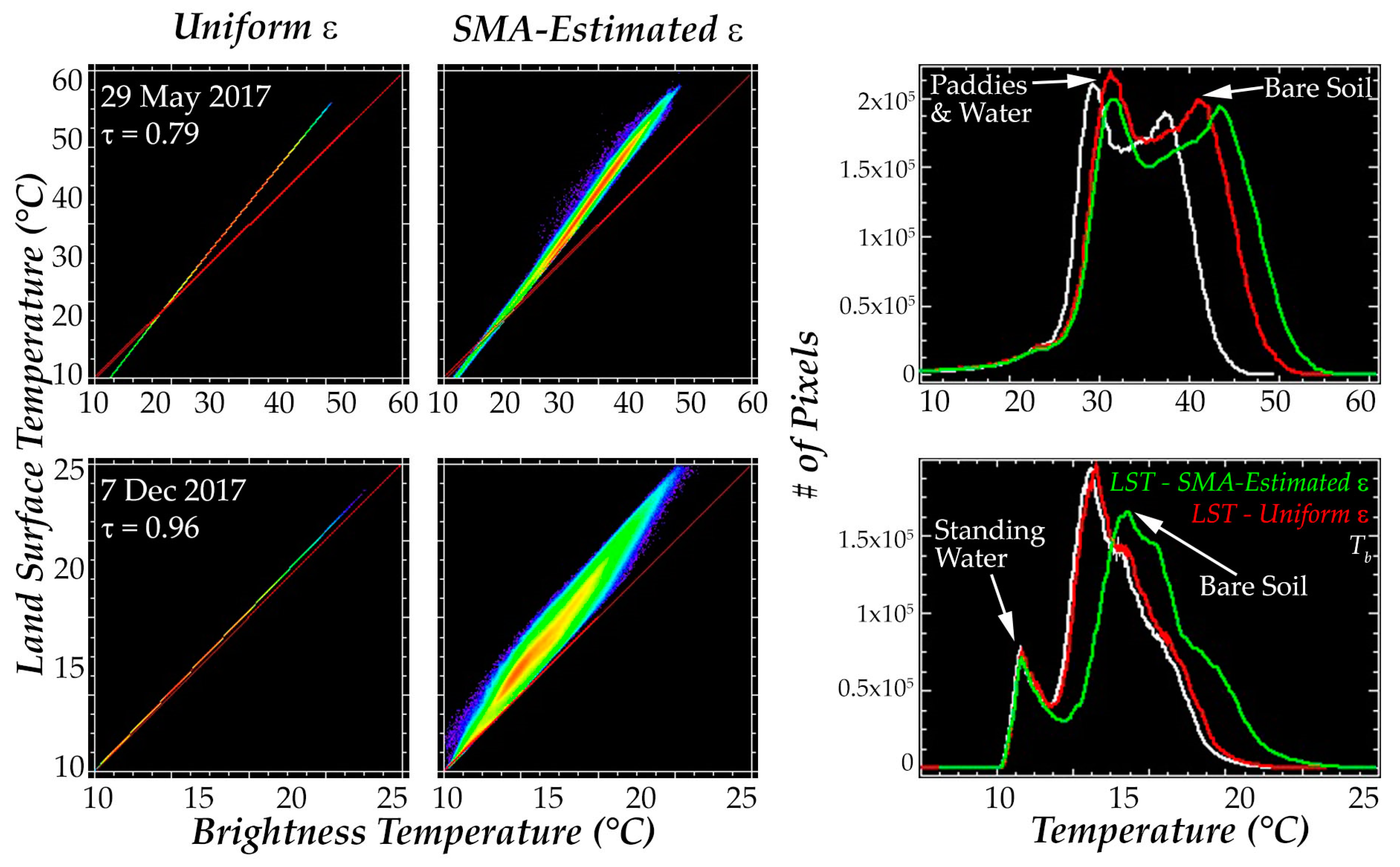
Figure 2 shows the effect of the atmospheric correction and pixelwise ε estimation on two representative scenes: one with a hot, low τ atmosphere (top row) and another with a cold, high τ atmosphere (bottom row). The estimated τ coefficients are 0.79 and 0.96, respectively, the most extreme values of the 22 scenes from 2016 and 2017 used in this study. The left column shows the effect of applying the atmospheric correction assuming uniform ε = 1, and the center column shows the effect of applying the atmospheric correction and estimating pixelwise mixed ε using SMA. Histograms of all three levels of correction for all image pixels in the field area are shown in the right column.
For the hot atmosphere, the effect of the atmospheric correction is essentially to act as a multiplicative linear transformation, decreasing the temperature of deep lakes by about 5 °C, increasing the temperature of rice paddies by about 2–5 °C and increasing the temperature of bare soil by about 5–9 °C. For the cold, high τ atmosphere, the effect is much smaller (less than 0.5 °C across all land cover types). The image-wide effect of the atmospheric correction is linear because the same linear coefficients are applied uniformly across the study area. In contrast, using pixelwise mixed ε introduces a more dispersive transformation because geographically explicit information is introduced. For the hot, low τ atmosphere, the overall amplitude of the atmospheric correction with pixelwise emissivity is approximately 10°C for bare soil, 4–6 °C for rice paddies, and 2–4 °C for deep lakes. The effects are reduced for the cold atmosphere, with temperature estimates for bare soil increasing by 2–5 °C, rice paddies by 0–2 °C, and deep lakes by 0–1 °C.
Additional insight into the relationship between radiative and kinetic temperature can be derived from comparison of satellite-derived LST versus field temperature data. In this study area, this can be achieved using measurements from the California Irrigation Management Information System (CIMIS). CIMIS maintains an extensive network of field observations of meteorological data throughout the agricultural regions of California. Figure 3 shows a map of the 4 station locations within the area of the white box from Figure 1. The stations bound the region dominated by rice agriculture (darker green) to the north, south and west. The stations are sited in agricultural microenvironments and include a comprehensive suite of air and soil temperature, rainfall, and wind measurements. These measurements are expected to be representative of the atmospheric and near surface conditions throughout the study area.
In Figure 3, daily time series of soil temperature (green) and air temperature (red) are plotted for the time of the Landsat 8 overpass for each of the stations, along with Landsat-derived Tb (gray) and LST (black) for each of the 9 pixels in a 3 × 3 box surrounding the station location. The variability in agreement between the field and satellite temperatures is likely related to variations in microclimate due to differences in the siting of each station. While all four stations are immediately surrounded by irrigated pasture, the Durham and Verona pastures are situated within a matrix of tree and row crops, while the Williams and Biggs pastures are surrounded by rice and/or wetlands. It is possible that the more saturated surface hydrology surrounding the Biggs and Williams sensors introduces atmospheric boundary layer effects that impact temperature retrievals. These local effects would not be captured by the atmospheric correction procedure used in this analysis.
As expected, in all cases the effect of the atmospheric correction is to increase the estimate of LST relative to the uncorrected Tb measurements. The magnitude of the increase is between 0.5 and 4 °C, depending on atmospheric transmission. Interestingly, while these corrections do amount to an overall bias shift of the LST time series 1 to 5 °C, they do not affect the relative spatiotemporal structure of time series or appreciably impact the amplitude of the annual cycle.
Regardless of these complexities, it is clear that the shape and rough amplitude of the Landsat LST time series generally agree with the station data, in some cases remarkably closely. With the exception of the anomalous 2017 Williams data, the amplitude of the difference between the field air temperature measurements and the satellite LST measurements is generally much smaller than the amplitude of the seasonal cycle. As expected, the LST is considerably higher than the soil T because the latter integrates over a depth of several cm of soil and is much less sensitive to the higher skin temperature of the soil surface. In all cases, the timing of the annual cycles of soil T, air T, Tb, and LST agree, suggesting that TIRS effectively captures the essential features of the thermal phenology.
2.6. Spatiotemporal Analysis and Temporal Mixture Models
Our approach to the quantitative analysis of satellite image time series is implemented in two stages: characterization and modeling. The two stages are summarized briefly below. Each stage is also presented separately in the Results section. For detailed background, explanation, and examples of implementation of the method, please see [18,44].
Characterization involves Empirical Orthogonal Function (EOF) analysis. EOF analysis is a general tool which can be applied to any image time series. For the purposes of this study, the time series of interest are sequential maps of fractional vegetation cover, Fv, and LST. EOF analysis considers each image time series as a matrix with each geographic pixel occupying a row and each time step occupying a column. A satellite image time series therefore contains a large (generally > 106) number of rows and a much smaller (generally < 103) number of columns. In the case of our study area, the number of rows is 12 × 106 (3000 × 4000 pixels) and the number of columns is 22 for the 2016 + 2017 analyses and 11 for the 2016-only analyses. EOF analysis is based on the Principal Component (PC) transform [45] which computes the covariance (or correlation) matrix of the data, then decomposes that matrix into its corresponding eigenvalue and eigenvector pairs. The eigenvectors show the dominant modes of uncorrelated spatial and temporal variance in the dataset, and the eigenvalues quantify the fraction of total variance associated with each mode. For more background on EOF analysis, see [46,47,48,49].
Characterization continues with the examination of the transformed spatiotemporal data in this new, optimized space, referred to as the Temporal Feature Space (TFS). The low order projections of the TFS are depicted graphically using scatterplots of the spatial PCs in conjunction with time series of the corresponding temporal EOFs. The most distinct temporal patterns (i.e., phenologies) occupy apexes of the data cluster in the TFS. The temporal patterns of the geographic pixels associated with these apexes are identified as temporal endmembers (tEMs). In the case of linear mixing, binary mixtures of these patterns occupy sharp edges between the apexes. Pixels in the interior of the point cloud can be represented as combinations of all the EM time series.
Once the temporal EMs are selected, the analysis proceeds to the modeling phase. By direct analogy to spectral mixture modeling, this analysis uses linear Temporal Mixture Models (TMMs, [50,51]) which have the virtue of relative mathematical simplicity and straightforward physical interpretation. Linear TMMs model every pixel time series as a linear combination of a small number of tEM time series. The tEMs to be used are identified during the characterization phase of the analysis. Inversion of the mixture model unmixes each pixel time series to yield an estimate of the relative contribution (fraction) of each tEM to each pixel time series in the dataset. The result is a set of continuous maps showing the relative contribution of each tEM pattern at each point in space. The meaning of the model result is therefore straightforward (quantitative description of similarity to each tEM), and the model inversion is mathematically transparent (ordinary least squares inversion of an overdetermined system of linear equations). This approach also has the benefit of generality, as no portion of the analysis imposes assumptions specific to particular geophysical variables or sensing modalities. The only implicit assumption is that spatiotemporal variance represents potentially useful information.
While this method has been shown to be effective in analyses using single geophysical variables (e.g., [18,44,50,51]), to our knowledge it has not yet been applied to coincident observations of reflectance and temperature. This study examines the implications and potential utility for parallel application of this spatiotemporal analysis methodology to the case of coincident LST and Fv image time series for the practical purpose of mapping and monitoring rice agriculture.
3. Results
The parallel analysis presented here requires additional characterization before the EOF analysis to examine and compare the spatiotemporal patterns present in each data stream. Section 3.1 and Section 3.2 show this initial step. Section 3.3 then presents the characterization as described in the Methods section, and Section 3.4 presents the results of the modeling step. Finally, Section 3.5 presents a potential application for near-realtime monitoring and results of field validation.
3.1. Vegetation Phenology
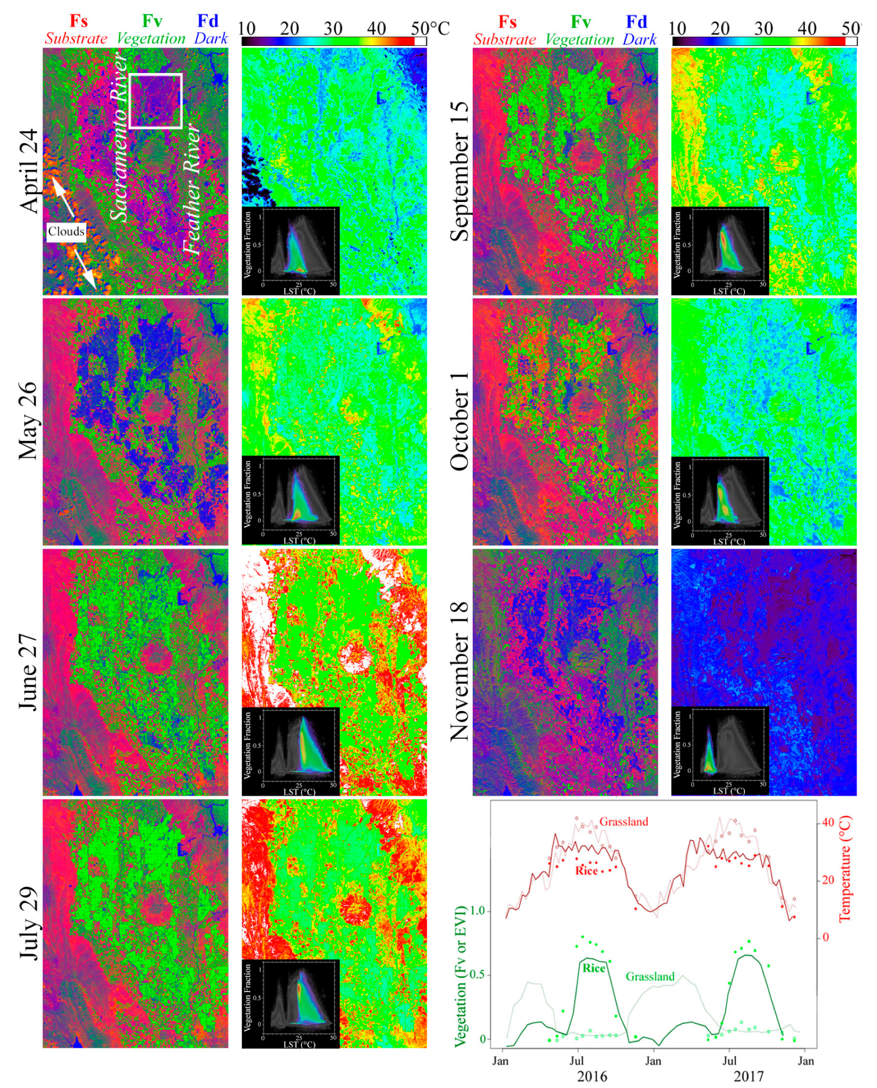
Figure 4 demonstrates a representative annual phenological progression of the region using a series of land cover fraction (first and third columns) and LST (second and fourth columns) images from the calendar year 2016. The subpixel fraction images use the colors Red, Green, and Blue to correspond to relative abundance of substrate (soil or non-photosynthetic vegetation), photosynthetic vegetation, and dark materials (shadow or water) for a given time. These relative abundances are computed using the 3-endmember spectral mixture model described in the Methods section. Each image is enhanced identically, so colors are directly comparable. Soils generally appear as red, photosynthetic vegetation as bright green, and standing water as blue. As vegetation senesces, its reflectance spectrum grades toward that of the substrate endmember, resulting in orange and yellow colors on the fraction images. Images are only shown from April through November, because winter months are generally covered in cloud and rice is not grown at this time.
Rice is generally grown in the clay rich soils to the east and west of the Sacramento and Feather River channels. The rice growing area can be visually identified as the area of standing water (dark blue/black) in the May 26 image. This is due to the rice crop phenology, summarized as follows:
Many, but not all, rice fields are flooded during winter (November through February or March) to provide habitat for migrating birds. In April, the flooded fields are drained, and all rice fields are plowed in preparation for the rice crop. Rice fields are then generally flooded in May and seeded by airplane into standing water. The rice then greens up during the summer months and begins to senesce in September, continuing to senesce and being harvested through September and October. By November, the harvest is complete. After harvest, some fields are left bare and others are flooded for winter bird habitat, and the cycle begins again. For more information on the rice cropping calendar in this region, see http://www.rice.ucanr.edu/ or http://www.calrice.org/.
While rice dominates the landscape, other vegetation also exists. The foothills of the Sierra Nevada, Coast Ranges, and Sutter Buttes largely host rainfed grasslands used for grazing. The phenology of these regions is nearly opposite that of rice agriculture, because the grasslands are green during winter and generally senesced during the summer months. In addition, a wide range of other row crops and orchards are grown in the valley with a diversity of cropping systems and phenologies. Settlements also occupy a small portion of the landscape, hosting an even more complex mixture of evergreen and deciduous trees, shrubs, and grasses.
The time series in the lower right of Figure 4 show typical phenological progressions of rice crops (solid) versus native grassland (dashed) in terms of both vegetation abundance (green) and temperature (red). As expected from the image time series, the vegetation abundance curves for the rice and grassland pixels are nearly 180° out of phase. Rice has a strong peak in vegetation abundance during the summer growing season, and also a minor peak during the winter fallow season, presumably from non-rice vegetation growing in flooded fields. The grassland pixels have very low amounts of photosynthetic vegetation during the hot and dry summer months because they are rainfed, but reach broad peaks during the winter rainy season of comparable but somewhat smaller amplitude than the agriculture. In Figure 4, dots correspond to Landsat Fv and LST observations and continuous curves correspond to MODIS EVI and LST time series. The benefit of using both MODIS and Landsat for purposes of this illustration is evident, in that there were no cloud-free Landsat images available over a 3-month period during the wintertime, but sufficient usable MODIS images were acquired to produce composites approximating the full annual time series.
3.2. Thermal Phenology
The fundamental physical process driving the thermal phenology of the region is the sinusoidal seasonal insolation curve, with an annual minimum at the winter solstice. However, the biogeophysical properties of the landscape modify this insolation curve in both space and time. For instance, grassland achieves a much greater summer temperature than rice because the land surface dominated by dry soil and non-photosynthetic vegetation (or absence of vegetation) has low thermal inertia, and can support very little evapotranspirative cooling. On the other hand, rice agriculture is not only irrigated but grown in standing water for much of the summer, resulting in substantial cooling both from evaporation of the paddy water below the canopy and transpiration of the respiring and photosynthesizing vegetation. This results in a relatively stable LST during the summer months, yielding a flatter top to the temperature curve.
The phenological progression of the thermal image time series complements that of the fraction image time series. In late April, the only prominent spatial patterns in the thermal field are due to elevation, rivers and lakes, and transient clouds. However, as the spring progresses into summer, clear differences emerge between rice and grassland areas. In the September and October images, differences within the region of rice agriculture become apparent, likely on the basis of evapotranspiration decreasing at variable rates as some fields senesce sooner than others, and some fields are drained before others to prepare for harvest. Once the fields are harvested, differences between land cover types are greatly reduced. In fall, the remaining vegetation can be somewhat warmer than its dry surroundings due to the greater heat capacity of its leaf water.
Finally, the scatterplots inset on the thermal images show the relationship between LST (x-axis) and Fv (y-axis) for every pixel in the image. These scatterplots are an alternate coordinate system with which to understand the dataset. The scatterplots are color-coded so warmer colors represent more pixels and cooler colors represent fewer pixels. The grayscale background silhouette of the full multitemporal point cloud shows the composite space of all the images together. Because so many pixels in the image correspond to rice agriculture, they generally form the largest cluster in Temperature vs Vegetation (TV) space and are represented by warmer colors. In April, for instance, rice fields are recently plowed so they are cool and unvegetated, and the corresponding warm colored cluster plots at the bottom center of the space. In May, the fields are flooded and become even cooler, but remain unvegetated, so the cluster moves to the left in TV space. In late June, fields vary widely from just planted (late crop) to nearly mature (early crop), resulting in a wide range of Fv. ET cools the crop so its temperature does not change appreciably, resulting in a vertically elongated cluster. For the rest of the summer, the fields do not change appreciably in vegetation abundance or temperature, so the cluster is stable until fields are drained and begin to senesce (September), resulting in the cluster elongating toward higher temperatures. Harvest of the rice crop results in a stepwise change of the TV properties of a rice field. The separation of the point cloud into two distinct clusters of approximately equal size (harvested & unharvested) in the October 1 image agrees with 2016 USDA estimates that 54% of the California rice crop was harvested by October 9 [52]. By mid-November, rice harvest is complete, and the landscape shifts into its winter state. Interestingly, the few usable winter images that exist plot in a nearly disjoint portion of the vegetation temperature space, suggesting that the spatial relationship between vegetation and temperature during winter may be dominated by fundamentally different physical processes than during summer.
3.3. Characterization—EOF Analysis and tEM Selection
The preceding figures can be summarized by the following set of observations:
- The thermal phenology of rice agriculture is substantially different in amplitude and shape from other land cover types in the region;
- The parallel evolution of both thermal and vegetation phenology can be explained in terms of the surface hydrologic cycle and growth cycle of the multiple phases of rice crops;
- The spatiotemporal variations in LST have substantial differences from those of the vegetation abundance, despite their interdependence; and
- The spatiotemporal variations in both LST and Fv can be explained using fundamental physical principles.
Put together, observations 1, 2 and 3 suggest that including Landsat LST in a phenological analysis could add information that is not present using vegetation abundance alone. Observation 4 suggests that such a phenological analysis could be based on straightforward physical principles with a bare minimum of model complexity.
One potential approach to this mapping problem is the spatiotemporal analysis method of [18]. A primary benefit of this approach is that it imposes no assumptions about the functional form of the phenology, but rather characterizes the temporal patterns based on the data itself. Other benefits to the method are its simplicity, robustness, and generalizability, as well as its ability to generate results with straightforward physical meaning. Because they are based on physical principles and easily identified tEMs representing known phenologies, maps derived from linear model inversion provide a degree of uniqueness of solution that is almost never provided by discrete thematic classifications which are based on ad hoc selection of land cover classes and training data.
In order to use this approach with a dual data stream, two decisions must be made. The first decision is whether to incorporate both streams into a single analysis or to analyze each in parallel. We present the results of parallel characterization method here because it is conceptually simpler and achieves the objectives of the current study. The combined characterization and analysis of thermal and vegetation phenology lends itself naturally to the study of ET dynamics, and is the focus of a separate study.
The second decision is whether to analyze the two years together or separately. Because significant benefits can result from either approach, we present results of both in Figure 5 and Figure 6, respectively. Because the two single-year characterizations yielded similar results, we present only the 2016 results as characteristic of both years of the dataset.
For each case, we begin by first conducting an EOF analysis of the relevant image time series. We choose unnormalized (covariance-based) rotations in each instance. Normalized (correlation-based) rotations were also investigated, but the resulting feature spaces were less informative. In each case, over 65% of the variance is represented in the first 3 dimensions of the data. While this number is low enough to suggest that informative structure may be present in the higher dimensions of the dataset, the three low-order dimensions capture the most relevant phenological patterns necessary to distinguish rice from other crops and to characterize its seasonal and interannual variability.
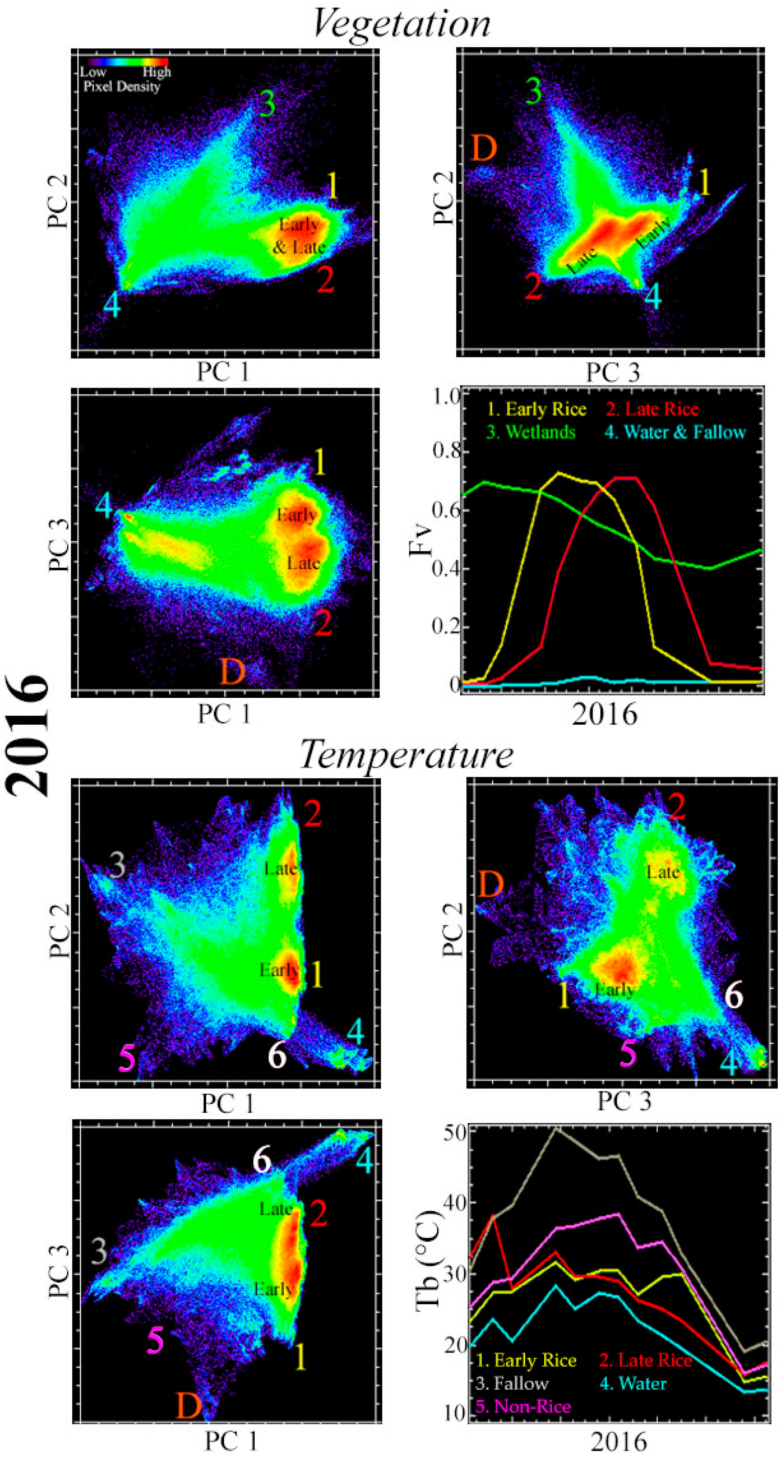
Figure 5 and Figure 6summarize the characterization stage of the parallel analyses for single year (2016) and dual year (2016 + 2017) time series, respectively. Characterization is based on the 24 × 24 km subset shown in the white box in Figure 4. We use this spatial subset because it is dominated by rice agriculture with a wide range of crop timing. In every case, the loadings of the first 3 spatial PCs are shown as scatterplots. These scatterplots represent the location of each geographic pixel in the image time series in a 3-dimensional space, known as the Temporal Feature Space (TFS), in which the axes represent the relative contributions of the first 3 EOFs (uncorrelated temporal patterns of maximum variance). Clusters in this space correspond to sets of geographic pixels with similar temporal trajectories over the course of the two years of the study. Apexes in the space correspond to temporal endmembers (tEMs), pixels with the most distinctive temporal patterns in the image time series. Pixel time series lying inside a convex hull connecting the tEMs can be represented as linear combinations of the tEM time series.
Figure 5 shows a comparison of the TFS for image time series of both Fv and LST for the year 2016. The TFS of the Fv image time series shows four distinct apexes representing the tEMs: Early Rice, Late Rice, Wetlands/Evergreen, and Water/Fallow. Time series of Fv corresponding to these tEMs are shown in the lower right. All 4 tEMs are clearly distinct on the PC 3 vs. 2 scatterplot. The point cloud in this scatterplot forms a cross shape, with the axis between tEMs 1 and 2 corresponding to phenological timing and the axis between tEMs 3 and 4 corresponding to overall vegetation abundance. The Water/Fallow tEM forms the sharpest corner, as expected given the small amount of variability expected in the Fv of water bodies and fallow fields through time. Early and Late tEMs are less sharp but still clearly defined, indicating substantial variability in the timing of the phenological signal. However, the Early and Late clusters are also visibly distinct, indicating two clear phenological groups. The Wetlands tEM is the most diffuse, as expected given the wide range of vegetation types, hydrological regimes, and land management strategies for wetlands in the area.
The TFS of the LST image time series shows substantially more clustering than that of the Fv time series. This indicates that more pixels have more similar LST trajectories than Fv trajectories. At least 7 tEMs are identifiable. The most distinct from each other are Water (EM 4; blue) and fallow fields (3; gray). Water time series are particularly distinctive as their very low PC 2 and very high PC 1 and 3 values position them as disjoint from the remainder of the dataset. The remainder of the space partitions into (a) differences in timing of rice phenology, and (b) differences between rice, non-rice agriculture, and wetlands. Wetlands (EM6) occupy the corner of the point cloud closest to water, and also form an axis grading into fallow fields (EM3). The Fallow-Wetland axis is nearly orthogonal to the Early-Late axis of rice phenology, most clearly seen in the PC 1 vs. 3 projection. Non-rice agriculture (EM5) plots on a continuum between the Early Rice and Fallow tEMs. Finally, double cropping (D) is clearly identifiable in both the Fv and LST feature spaces. Few fields in the spatial subset used for this rotation practice double cropping, so this tEM is sparsely populated.
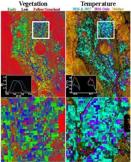
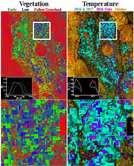
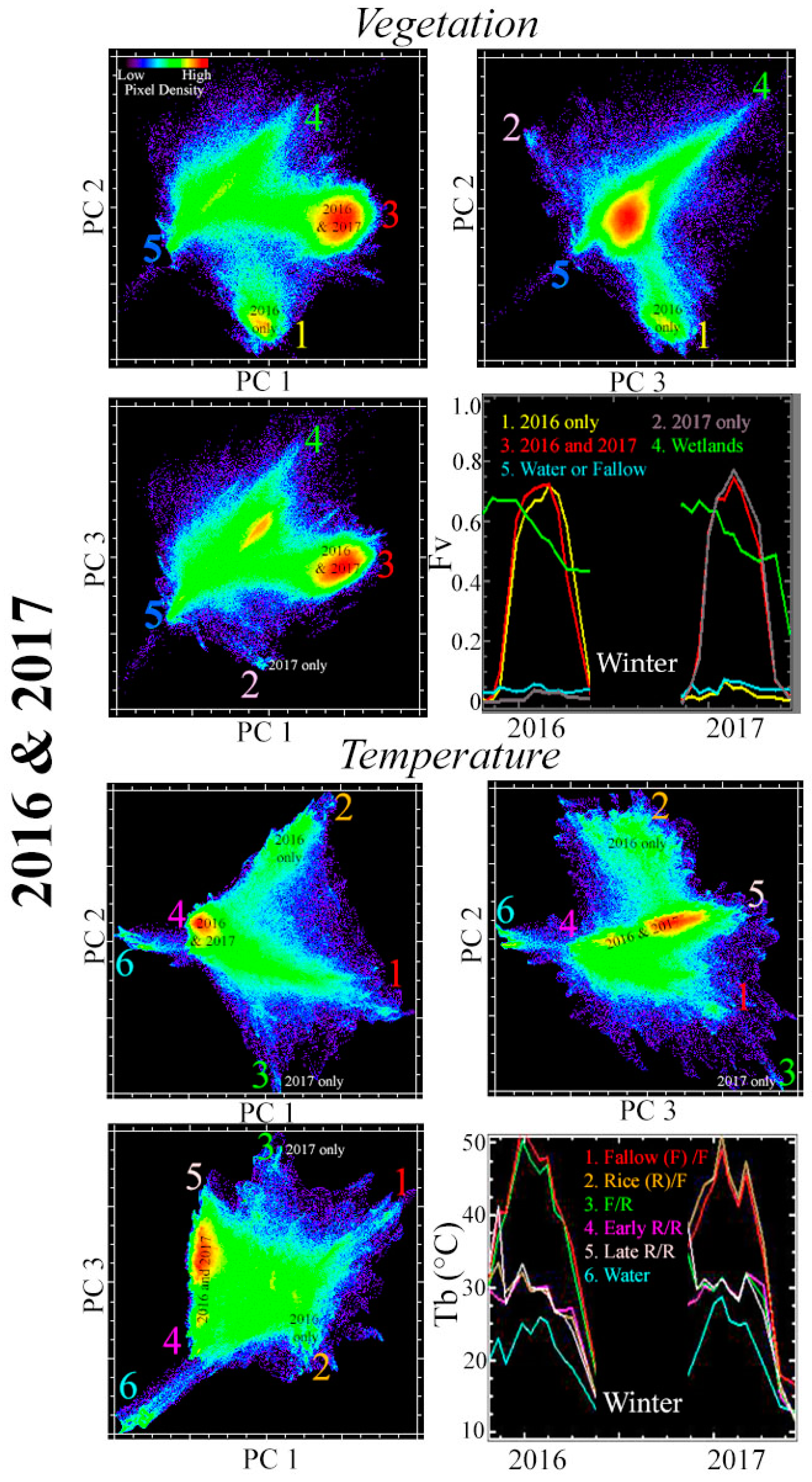
Figure 6 shows a characterization of the dual year 2016 + 2017 image time series. In both time series, the early/late phase information that dominated the single year time series is suppressed (though still present), and the structure of the TFS is dominated by year-to-year differences in crop presence or absence. In the Fv space, both Wetlands (EM4; green) and Water/Fallow (EM5; blue) are still clear tEMs. The largest cluster, however, is now that of fields cropped in both 2016 and 2017 (EM3; red). This cluster is clearly distinct from the small cluster of fields cropped in 2017 only (EM2; gray) and the much larger cluster of fields cropped in 2016 only (EM1; yellow). The fact that the 2016-only cluster is much larger than the 2017-only cluster is concordant with official USDA estimates of 42,000 fewer acres of California rice planted in 2017 than 2016 due to higher prices for competing commodities and severe early season flooding [53,54].
The dual year LST space again shows more clustering and overall complexity than the corresponding Fv space. At least 6 tEMs are identifiable. Again, the greatest distinction exists between water and fields that are fallow in both years (F/F). Water time series are again particularly distinctive as their very low PC 1 and PC 3 values position them as disjoint from the remainder of the dataset. The remainder of the space partitions into (a) differences in timing of phenology for fields under rice cultivation in both years, and (b) the presence and absence of a rice crop in each year. The axis corresponding to phenology is nearly orthogonal to the axis corresponding to presence/absence of crop in each year. The potential utility of this information is discussed below.
While information about the phase of the rice is clearly present in both single year datasets, the Fv space tEMs capture more end-of-season variability than the LST tEMs. This could be due to gradual browning of the top canopy layer over weeks to months (resulting in progressive decline in Fv over the second half of the growing season) being accompanied by continual cooling by ET of the green vegetation and paddy water below (resulting in minimal change of LST). However, the LST dataset clearly shows enhanced ability to discriminate between rice and non-rice crops, likely due to early season paddy water producing a unique signature in LST but not Fv. For the dual year characterization, both Fv and LST clearly discriminate between areas cropped both years versus each individual year, but again LST shows superior ability to discriminate between rice and non-rice crops. Clearly, analyzing both datasets in parallel may yield substantial benefit over only using one, especially given that the two are co-acquired in all standard Landsat image acquisitions.
3.4. Modeling
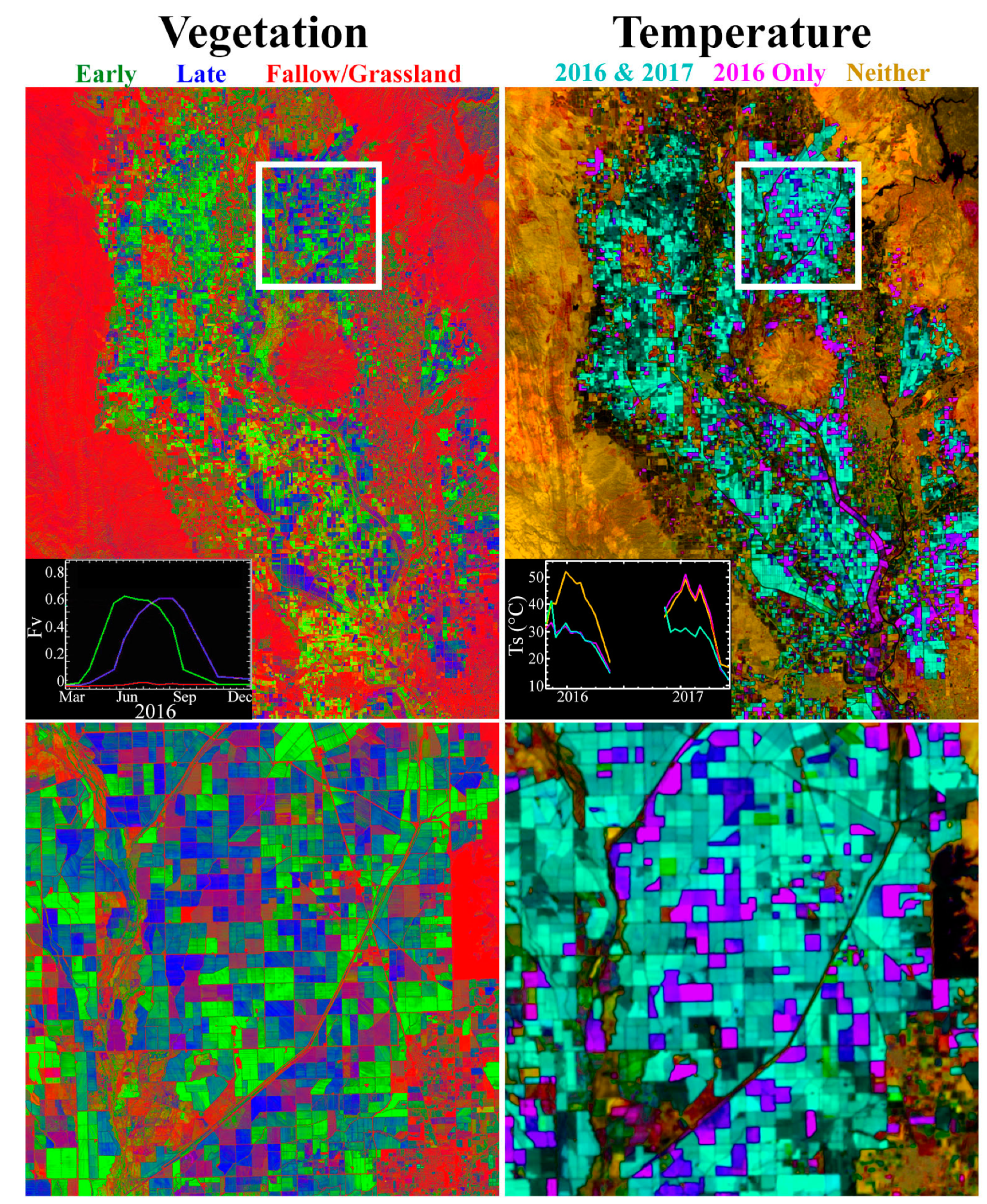
As described in the Methods section, tEMs selected from each TFS were then used as the basis for two separate linear temporal mixture models. These models were then inverted to produce maps of thermal and vegetation phenology. Figure 7 shows the result of these inversions. In this figure, the saturation of each color corresponds to the similarity of each pixel to each of the tEM time series. Greater saturation implies greater similarity to the corresponding tEM (or binary mixtures for subtractive colors), while less saturation implies less similarity of the corresponding pixel to any of the tEMs. The latter is associated with higher model misfit, and is expected for pixels with phenologies not included in the model. Individual fields are clearly identifiable as either very early (pure green), very late (pure blue) or a mixture of the two (dark cyan). Intrafield heterogeneity in phenology is also clearly present in some cases, showing portions of individual fields growing faster than other portions. The potential utility of Landsat’s ability to resolve intrafield spatiotemporal variability is discussed below. Overall, RMS misfits were comparable but somewhat higher for the Fv (μ = 0.15, 90% < 0.25) than the LST (μ = 0.07, 90% < 0.12) models. While these model misfit values are higher than generally observed for spectral mixture models, this is expected given the phenological complexity of the landscape and the relatively low number of tEMs used.
The right column shows the result of a 3 tEM temporal mixture model of 2016 + 2017 thermal phenology showing crops in both years (cyan), only 2016, magenta, or neither (dark yellow/orange). The unique temporal signature of rice thermal phenology allows it to be readily identified from other types of agriculture, which map as dull colors corresponding to combinations of tEMs. Field-to-field variations in the similarity of each pixel time series to the tEMs are present, likely due to a combination of soil moisture during the fallow year and/or greenup phase during the cropped year. Some intrafield variability is also present, likely for similar reasons.
While the Fv TMM maps crop timing with high accuracy, it does not explicitly distinguish between rice and non-rice agriculture. As a result, non-rice agriculture maps in a variety of ways, potentially mimicking rice, depending on its phenological characteristics. Fortunately, the thermal image time series can explicitly capture the phenological signature of rice by leveraging the large early-season difference between cold, flooded, recently planted rice fields and hot, dry, recently planted non-rice fields. Interpreting the two of these phenology maps together therefore provides maximum information about both the location and timing of rice agriculture.
3.5. Near-Realtime Monitoring & Field Validation
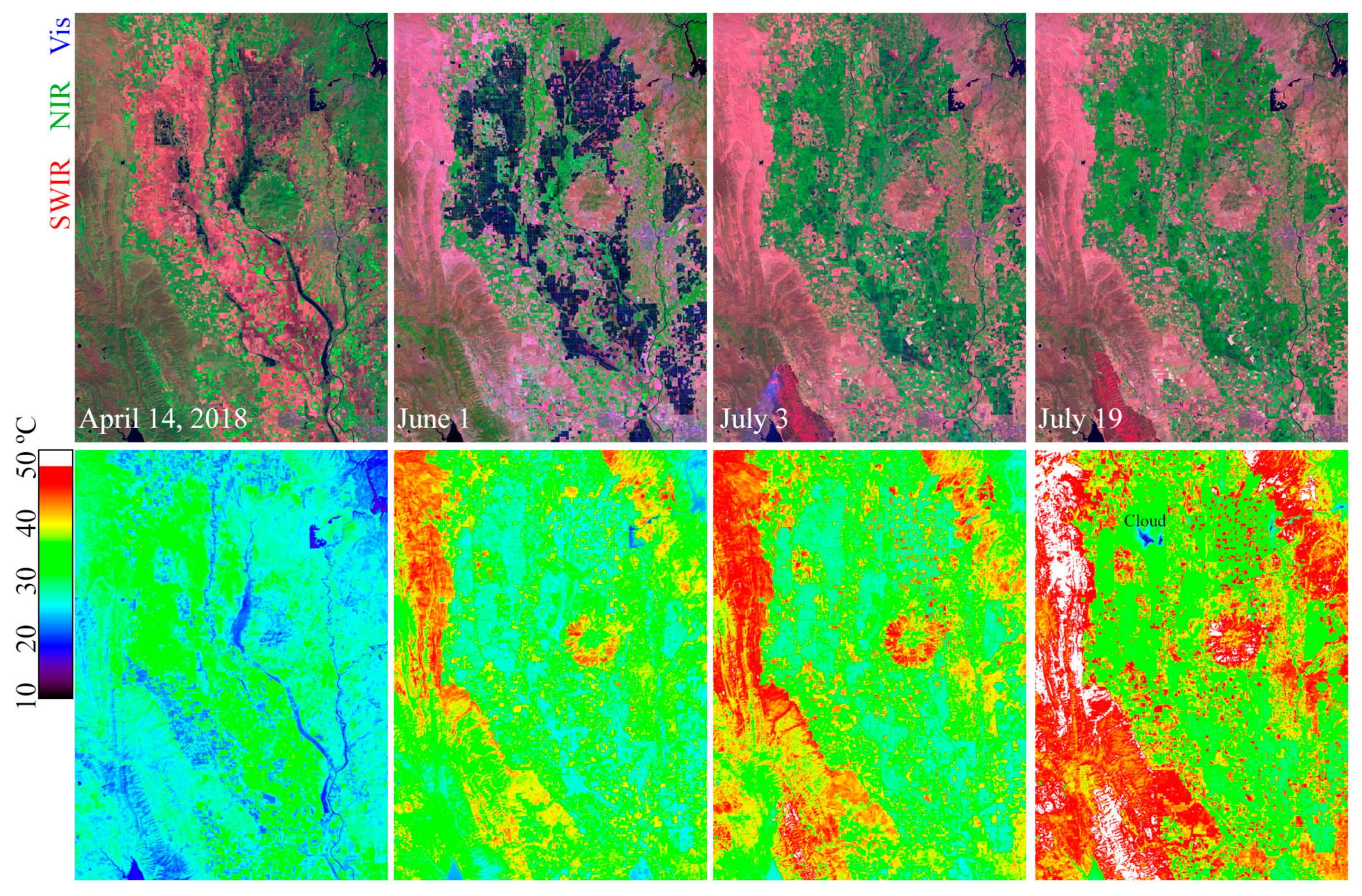
To illustrate one potential application of this methodology, we present the results of a TMM generated in the middle of the current (2018) growing season. 2018 presents an unusually challenging case for the model, because only the first part of the growing season is available, with only 2/3 as many usable images as the same period in 2016 and 2017. This is due to the prevalence of cloud cover in many spring images and smoke plumes from multiple severe wild fires in late summer images. Through the end of July, only 4 usable thermal images were collected, in comparison to 6 images through the end of July for each of the 2016 and 2017 growing seasons.
Figure 8 shows false color composite and thermal image time series for these 4 images. The false color composite images show a clear difference in crop timing between the rice growing areas in the eastern versus western portions of the valley, with the dividing line located approximately at the Sacramento River channel in the north and the Sutter Bypass in the south. The wide range of planting times in 2018, and the overall unusually late crop, is due to complex water management circumstances. Because of the relatively dry winter and associated low reservoir levels, uncertainty existed in early spring about expected water allocations. Heavy April rains then boosted allocations, but also forced farmers to wait for the clay-rich soils to dry before it was possible to bring tractors onto the fields for leveling. The fields which had already been prepared could be flooded and planted on time, but those which had not were forced to plant significantly later than usual. This is described in brief by [55], and expected impacts of this situation are broadly described by [56].
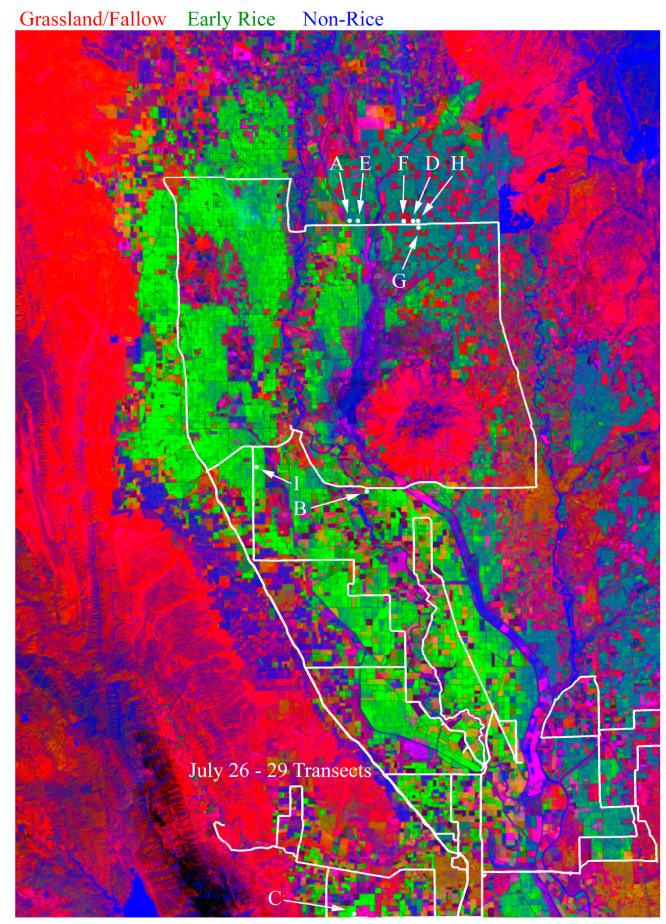
A TMM condenses the information from these 4 LST images into a single map, shown in Figure 9. In this model, red corresponds to grasslands and fallow fields, green corresponds to early rice, and blue corresponds to water and non-rice crops. Despite the limited data availability in 2018, and the fact that this map is produced mid-season with no data on senescence or harvest, the areas growing rice are clearly identifiable. The broad east-west dichotomy in planting date described by [55] is evident in the discrepancy between bright and dull green map color. Field validation with 1650 km of driving transects, 8500 field photos, and 380 field spectra verifies that 527 of 592 fields (89%) are correctly mapped as rice. Validation details are given in the Appendix.
4. Discussion
The topological structure of the low order temporal feature spaces provides a detailed yet intuitive characterization of the thermal and vegetation phenology of the 2016 and 2017 rice crops in the Sacramento Valley. The clearly distinct temporal endmembers spanning the feature space correspond to distinctive and easily verified land cover phenologies with straightforward interpretations in terms of vegetation abundance and LST at decameter scales. The degree of separation of the temporal endmembers, and the fact that they bound almost all the pixels in the feature spaces, allows them to be used as the basis for useful linear mixture models that can be inverted to yield pixel scale similarity metrics for each temporal endmember. The resulting endmember fraction maps provide continuous field estimates of both vegetation and thermal phenology of multiple rice crops as well as other land cover types. While the continuous field maps provide the most information on the spatiotemporal evolution of the rice crops, the clear presence of distinct clusters within the temporal feature spaces shows that the continuous field maps could be easily discretized into thematic classifications if necessary. The spatiotemporal clustering highlights clear distinctions between the multiple phases of rice cropping, as well as from other land cover types with different phenologies. It is important to note that continuous fraction land cover models can be used to accurately represent compositionally discrete land cover (like agriculture) with no loss of generality, but the converse is not true. Discrete thematic classifications cannot accurately represent the far more common diversity of continuously varying land cover properties present in most landscapes.
The ability to rigorously map and monitor the state of rice agriculture with optical satellite imagery has a wide range of potential implications:
4.1. Harvest Forecasts
In many regions of the world, the prediction of rice harvest is hindered by inaccurate estimates of basic information. While providing accurate estimates of yield from satellite imagery can be difficult because of the range of factors that can contribute to the harvest, it is likely that constraints on fundamental variables such as planting date and total area under cultivation could be improved with the joint VSWIR + TIR temporal mixture model approach presented here. In particular, TMMs based on single-year time series show the potential to map crop timing, and dual-year time series show the potential to identify changes in the location and overall abundance of planted fields. This could improve one set of inputs to complex yield models, which also rely on a significant amount of additional ancillary information, as well as work synergistically with other rice crop monitoring systems such as the methodologies proposed by [17,57,58].
4.2. Intra-Field Variability: Weed and Nutrient Managament
Examination of decameter image time series from sensors such as Landsat and Sentinel reveals considerable intra-field heterogeneity in the time series of green-up and senescence. These within-field variations likely arise as a result of imperfections in field leveling, flooding, and drainage; variability in weed and nutrient management; and heterogeneity in planting density. The information present in these variations could be leveraged using active management strategies for precision agriculture. In conjunction with unmanned autonomous vehicles, localized application of fertilizer and herbicide could be targeted to areas of concern with a potentially significant reduction in environmental impact and cost to the grower. The growing prevalence of VNIR hyperspectral imaging sensors has the potential to contribute significantly to these problems by discriminating between individual absorption features, such as those captured by the field spectra shown in Figure A1 of the Appendix.
4.3. Pest Management
Some pests require proximity in order to transmit from one field to another. Large, interconnected regions growing similar crops may provide transmission opportunities for these pests. Transmission could be minimized by a basin-scale management approach based upon strategic disruption of spatial networks of agriculture. Accurate crop-specific maps could provide a useful input into a network-based approach to understanding agricultural landscape evolution, as explored in [59].
4.4. Evapotranspiration and Water Use
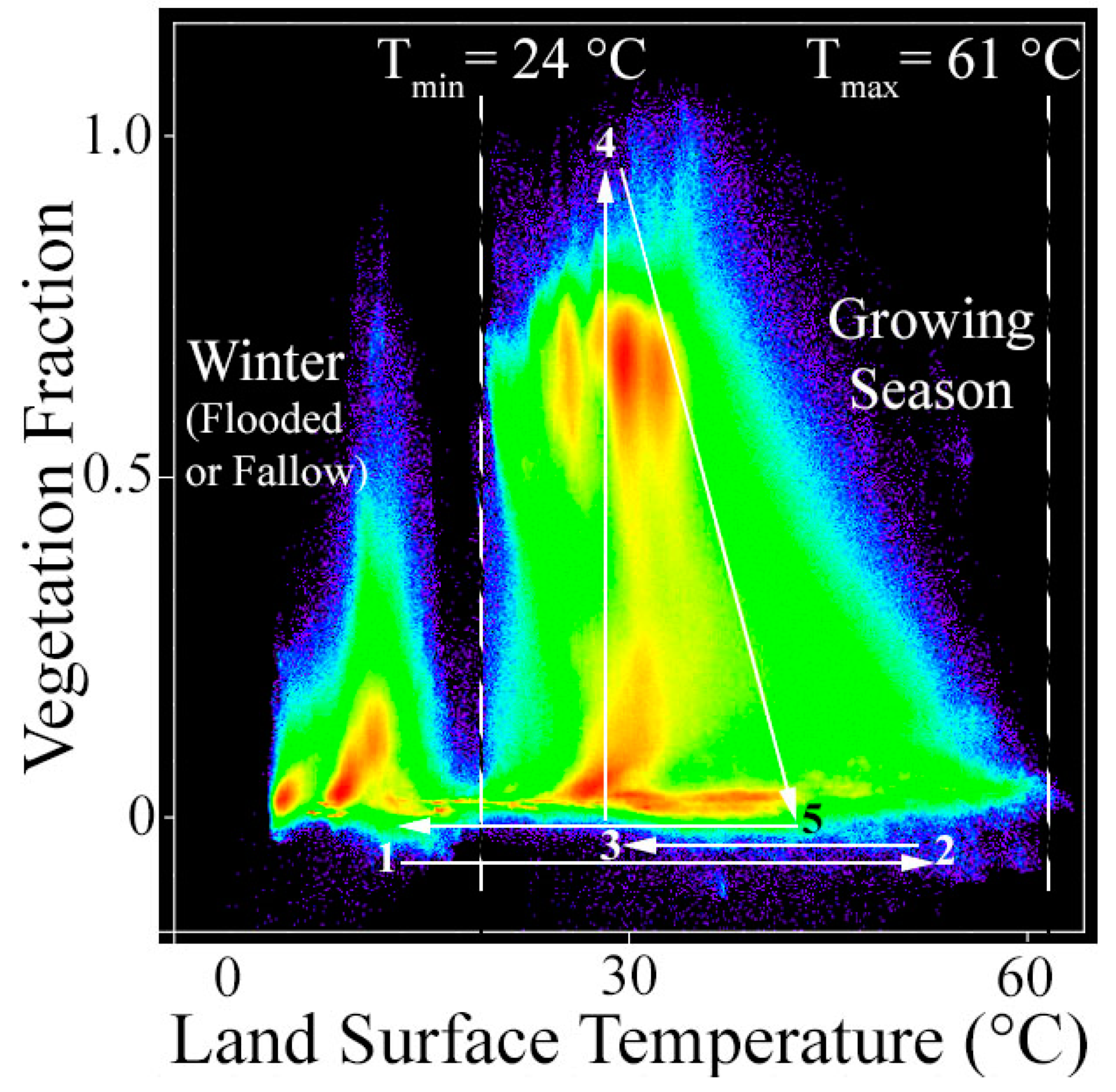
ET has been shown to be remarkably consistent for rice fields throughout the growing season [60]. Indeed, the relative stability of the LST and area of illuminated photosynthetic vegetation of rice fields are a part of the reason why the joint VSWIR + TIR mapping approach is so well-suited to rice in particular. This is shown explicitly in the spatiotemporal composite TV space for all 22 images in the 2016–2017 time series, shown in Figure 10.
The composite TV space shown in Figure 10 is particularly illuminating when viewed in relation to its subsets shown earlier in Figure 4. The wide range of LST values shown at near-zero Fv is primarily due to the substantial discrepancy between the relatively high heat capacity of water and the much lower heat capacity of dry soil (and synthetic surfaces like pavement and plastics). In contrast, the much more constrained range of values at high Fv values is likely a reflection of the thermal stability of dense, well-watered, respiring vegetation. The warm-colored clusters in this space represent groups of geographic pixels with similar TV properties. At low values of Fv, these are likely bare fields with similar moisture contents and tilling practices. In contrast, the clustering at high Fv values likely corresponds to rice fields imaged at different dates, with differences in water temperature resulting from fluctuations in air temperature due to changing weather within the growing season.
At least two additional features of this plot suggest potential avenues for future work through application to ET, following the Triangle Method introduced by [61], further elaborated by [62], and recently reviewed by [63] with additional useful explanation in [64]. First, the remarkably straight edges suggest the Sacramento Valley may be particularly well-suited to this approach to ET mapping. This is likely due to a combination of large field sizes, prevalent irrigation, and dominance of agricultural land use across the landscape. Second, a clear division between the growing season and the winter is also evident, suggesting the relationship between temperature and vegetation can be described as alternating between (at least) two physical regimes over the course of the year. Moving forward, the application of the spatiotemporal analysis methods described in this paper to image time series of quantities estimated by ET models has the potential to make progress toward all 5 of the requirements of the Path Forward outlined by the recent Decadal Survey [20], especially viewed under the unifying framework of spectral mixture analysis, as proposed by [19]. Detailed intercomparison of ET estimates from this and other ET models presents an attract avenue for future work.
4.5. View Angle and Flooding Presence
Because rice is an erectophile plant, small differences in off-nadir viewing geometry can produce significant differences in its overall bidirectional reflectance distribution function (BRDF). Specifically, the background of paddy water or soil is most pronounced when nadir-looking and rapidly exits the field of view when viewed off-nadir. Sufficient data now exist to quantify this effect at various stages throughout the rice life cycle. Understanding the size of this effect has the potential to determine at what stages of development the flooding or drying of the substrate below the rice can be accurately determined, with potential implications for the verification of alternative cropping practices such as alternate flooding and draining of fields.
4.6. Integration of New Data Streams
Finally, recent missions such as the ECOsystem Spaceborne Thermal Radiometer Experiment (ECOSTRESS), as well as the planned launch of hyperspectral missions such as NASA’s Surface Biology and Geology (SBG) and DLR’s EnMap, have the potential to substantially enhance the ability of the scientific community to map and monitor rice agriculture. During crop growth, VSWIR imaging spectroscopy has been shown to provide information about biomass [65] and foliar chemistry such as nitrogen and cellulose [66], and multispectral thermal measurements are expected to provide improved measures of evapotranspiration [67]. Hyperspectral measurements have also been shown to be potentially useful for detecting physiological stress in rice due to soil heavy metal content [68], fungal infections [69], and insect infestations [70]. When fields are fallow, hyperspectral measurements are expected to provide improved soil characterization [71,72]. It is possible that when this information is incorporated in temporal mixture models, it could potentially provide useful added information about the presence, timing, and spread of pathogens across a landscape; the need for fertilizer application; and/or water consumption and stress across rice and non-rice agricultural landscapes.
5. Conclusions
The combined spatiotemporal analysis of decameter scale VSWIR and thermal imaging shows considerable promise for improvements in the mapping and monitoring of rice agriculture. Characterization of single-year time series of the agriculture-dominated Sacramento Valley of California readily yields information about early/late crop planting, while dual-year characterization provides information about year-to-year crop conversion. Surprisingly, considerably more clustering is evident in the LST image time series than in the Fv image time series, in both single- and dual-year cases. Investigation of the temporal feature spaces suggests that Fv time series data show particular promise for estimating crop timing, while LST appears particularly well suited for distinguishing rice from other crops. Example monitoring results from the 2018 growing season show considerable promise for near-realtime mapping of rice phenology using partial-season TMMs. Field validation based on over 1650 km of driving transects and 8500 field photos confirms that mid-season monitoring models can provide an accurate upper bound estimate (<1% false negatives; 11% false positives) of the spatial extent and relative timing of the rice crop, even under conditions of relative data scarcity (only 4 images total for 2018, with only 1 capturing flooded and unplanted rice paddies). These results could have potential implications for food security, precision agriculture, pest management, and ET.
Author Contributions
Conceptualization, D.S. and C.S.; Formal Analysis, D.S.; Funding Acquisition, D.S. and C.S.; Investigation, D.S. and C.S.; Methodology, D.S. and C.S.; Supervision, C.S.; Writing—Original Draft, D.S.; Writing—Review & Editing, D.S. and C.S.
Funding
Work done by DS was conducted with Government support under FA9550-11-C-0028 and awarded by the Department of Defense, Air Force Office of Scientific Research, National Defense Science and Engineering Graduate (NDSEG) Fellowship, 32 CFR 168a. CS was supported by the NASA MultiSensor Land Imaging program (grant NNX15AT65G).
Acknowledgments
DS thanks B. Linquist and T. Rehman for a helpful and productive conversation, J. & E. Raney for geotechnical expertise and illuminating field observations, and F. & L. Sousa for local geographic expertise and field assistance.
Conflicts of Interest
The authors declare no conflict of interest.
Appendix A. Field Validation
The TMM for the 2018 growing season shown in Figure 9 is validated with over 1650 km of field transects collected between July 26 and 29 (white lines), including over 8500 field photos and 380 VNIR reflectance spectra. Field spectra are mapped as white dots and will be discussed further in Figure A1. Comparison of field photos to map output shows the model to produce < 1% false negatives (i.e., fields planted as rice but not captured by the model). However, approximately 11% of fields in the model were identified as false positives (i.e., fields in which rice was not planted, but mapped by the model as rice). The reason for the prevalence of false positives in the 2018 model is straightforward, as only 1 image captures the rice in the phase in which it is dominated by standing water. Because the thermal signature of standing water can sometimes be similar to that transpiring vegetation and wet soil, the thermal time series of any crop which was bare in mid-April but already fully green (or fallow and saturated) by June 1 could mimic that of the rice. This thermal mimicking is expected to be less severe in years with better data availability, and could also potentially be resolved by building a more complex model in which both Fv and LST are used. However, for the purposes of simplicity and illustration of the method outlined in this work, we defer a detailed examination of the strengths and weaknesses of more complex models to a future study.
VNIR field spectra were collected with an ASD HandHeld2 field spectrometer on July 29. Wildfires were active in the Coast Ranges to the west and north of the study area from mid-July through late August, 2018. As a result, substantial atmospheric contamination was present during field spectra collection. These effects are evident in satellite images collected before, during, and after the field campaign. When compared to both same-day Sentinel-2 spectra (corrected with the ESA Sen2Cor algorithm) and Landsat 8 spectra from August 4, 2018 (corrected with the NASA/USGS LaSRC algorithm), the field measurements yielded higher reflectance across all wavelengths than the satellite spectra. We interpret this as resulting from substantial indirect illumination by haze from the fires, view angle discrepancies due to the field spectrometer being held slightly off-nadir, and the unavoidable difference in measurement distance between the Spectralon white standard (used for calibration) and the distance from the rice canopy necessary to sample a representative mixture of foliage and exposed paddy water (or soil). Fortunately, however, the phenological progression can be captured by relative differences in reflectance between wavelengths. In order to facilitate comparison of spectral shapes, the overall amplitudes of the field spectra were adjusted by simple multiplicative scaling using constants in the range 0.5 to 0.8.
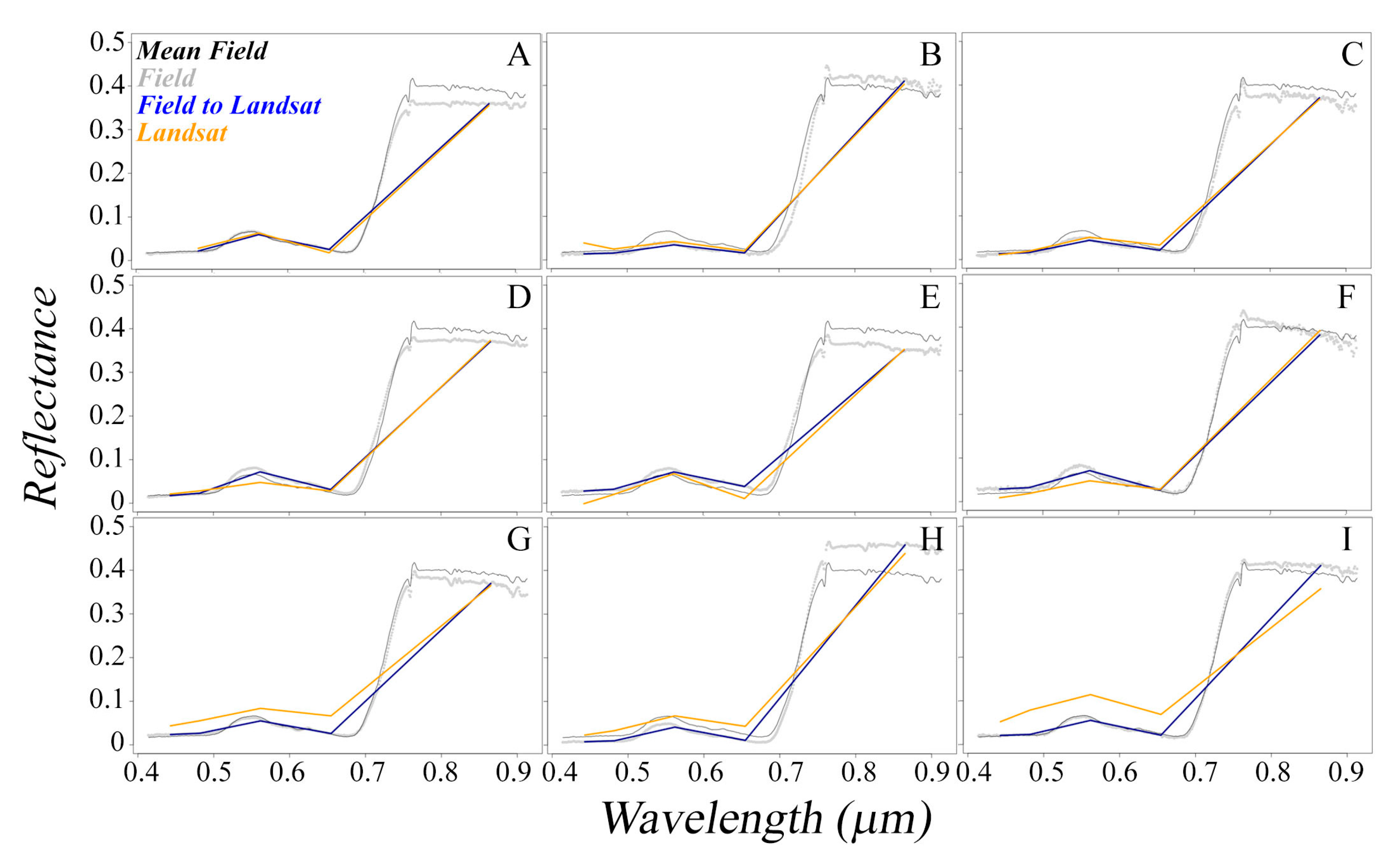
Figure A1 shows the corrected field spectra at full spectral resolution (thin gray) and the mean spectrum (thin black) for reference, as well as these spectra convolved with the broadband spectral response functions of the VNIR bands of the Landsat 8 OLI sensor (thick blue). These are shown in comparison to the actual observed Landsat 8 spectra from the August 4 Landsat 8 image (thick gold). In some cases (A–C), the agreement between the synthetic and observed Landsat spectra is remarkably good, even despite the significant atmospheric problems discussed above and the nearly 1 week between field and satellite data collection. In other cases, the spectral shape at visible wavelengths is distorted (D–F) or there is an overall loss of contrast (G–I) in the satellite spectra. These imperfections are likely due a combination of (1) changes in the state of the atmosphere in the 10 s of seconds between field calibration to white standard and collection of reflectance spectra, and (2) the inability of the atmospheric correction model to capture the complex scattering and absorption effects of the smoke plumes.
In addition to the comparison with broadband observations, field spectra show subtle features which are not captured by multispectral instruments. Changes in absorption depth in the visible red are likely due to chlorophyll b and other plant pigments. In addition, changes in the curvature at the base of the red edge (0.69–0.71 µm), as well as variations in slope at the top of the red edge (0.8–0.9 µm) have the potential to be leveraged in future work for investigations into nutrient stress and phenological progression of plant functional traits.
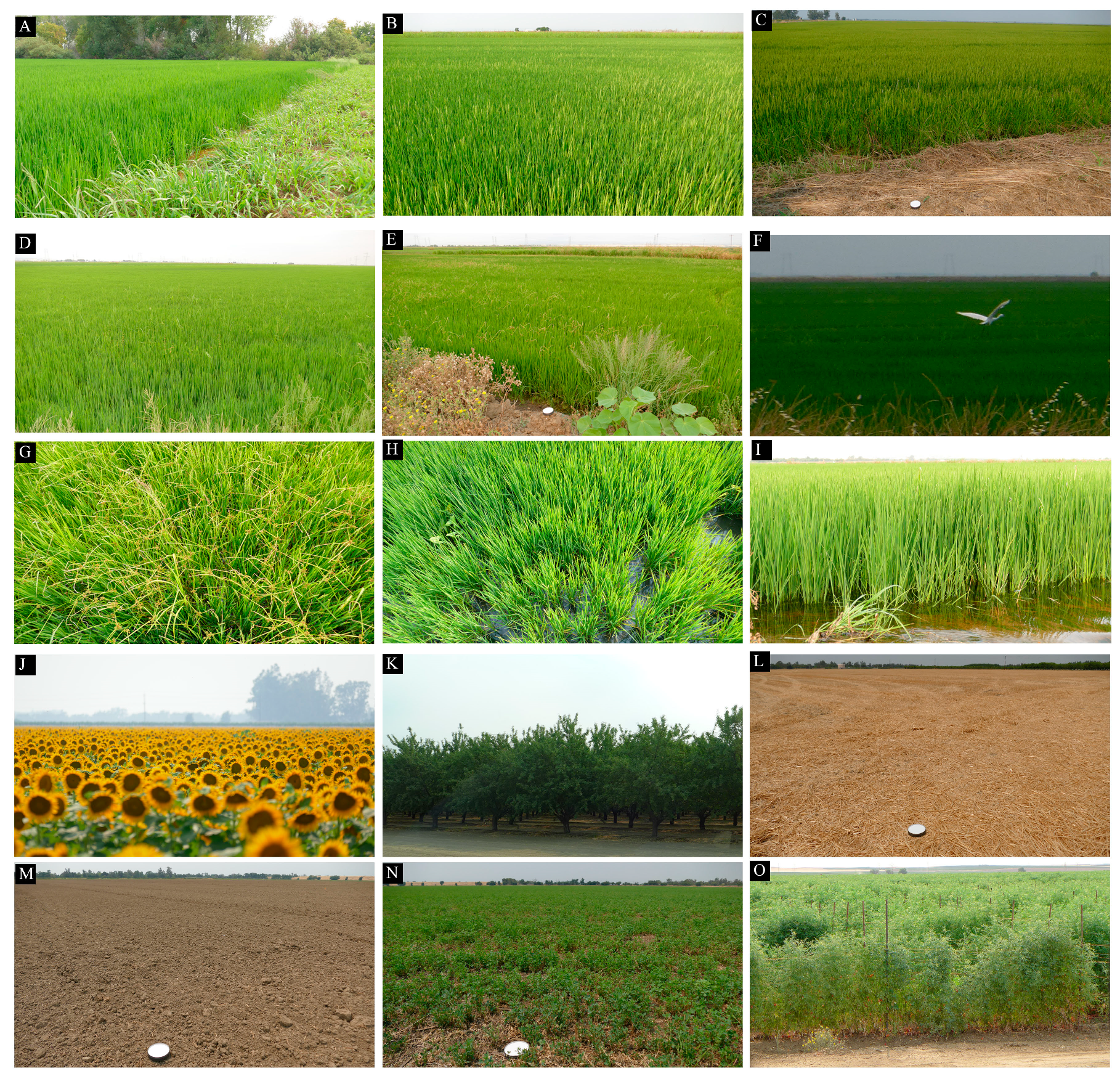
Finally, sample field photos showing rice at a variety of stages are shown in Figure A2. In late July, 2018, rice in the Sacramento Valley was observed in a range of maturity stages (photos A–C). The prevalence of weeds widely varied among fields (D and E). Abundant waterfowl (F) could be observed feeding in the rice fields. Viewed from above, weedy rice fields (G) were clearly distinct from weed-free fields (H). Substantial standing water background was observed in nadir-looking photos. The importance of view angle can be clearly seen when comparing (H) and (I), as rice fields of this age are fully opaque when viewed obliquely but not when viewed from nadir. A broad diversity of other agricultural land covers was also present in the valley, including sunflowers (J), fruit and nut orchards (K), rice straw (L), bare soil (M), alfalfa (N) and tomatoes (O).
Figure A1.
Comparison of field and satellite spectra. Continuous field spectra (light gray) were collected on July 28 and 29 at 9 rice fields, then convolved to bands 2-5 of the Landsat 8 OLI sensor (blue). These are then compared with actual Landsat spectra from the same locations imaged on August 4 (gold). The Landsat spectra were atmospherically corrected with the standard LaSRC atmospheric correction. In some cases (A–C) the synthetic and observed Landsat spectra agree remarkably well, especially given the pervasive atmospheric effects due to fires present during both the days of field measurement and satellite overpass and the nearly 1 week of time elapsed. In other cases (D–F), the overall ranges of the spectra are similar but the shape in the visible is notably distorted. In yet other cases (G–I), loss of contrast is observed, likely due to aerosol contamination incompletely corrected by the LaSRC model. Locations of field spectra are shown in Figure 8.

Figure A2.
Photos from July 2018 field validation campaign. In late July, rice was present in a wide range of stages from not yet headded (A) to partially and fully headded (B,C). Weeds were visibly present at a range of abundances in some fields (D,E). Waterfowl (F) continue to hunt in the rice paddies during the growing season. Viewed from near nadir, weeds (G) and standing water below the rice plants (H) are clearly visible. The importance of view angle is clearly evident when comparing these photos to side-on photos like I. A wide range of other agricultural land covers is present in the valley, including sunflowers (J), fruit and nut orchards (K), wheat stubble (L), bare fields (M), alfalfa (N) and heirloom tomatoes (O).

References
- Muthayya, S.; Sugimoto, J.D.; Montgomery, S.; Maberly, G.F. An overview of global rice production, supply, trade, and consumption. Ann. N. Y. Acad. Sci. 2014, 1324, 7–14. [Google Scholar] [CrossRef] [PubMed] [Green Version]
- Global Rice Science Partnership. Rice Almanac, 4th Edition: Source Book for One of the Most Important Economic Activities on Earth; International Rice Research Institute: Los Banos, Philippines, 2013. [Google Scholar]
- Bolton, D.; Friedl, M. Forecasting crop yield using remotely sensed vegetation indices and crop phenology metrics. Agric. For. Meteorol. 2013, 173, 74–84. [Google Scholar] [CrossRef]
- Anderson, M.; Allen, R.G.; Morse, A.; Kustas, W.P. Use of Landsat thermal imagery in monitoring evapotranspiration and managing water resources. Remote Sens. Environ. 2012, 122, 50–65. [Google Scholar] [CrossRef]
- Wilcox, C.; Frazier, B.; Ball, S. Relationship between soil organic carbon and Landsat TM data in Eastern Washington. Photogramm. Eng. Remote Sens. 1994, 60, 777–781. [Google Scholar]
- Shaw, D.R. Translation of remote sensing data into weed management decisions. Weed Sci. 2005, 53, 264–273. [Google Scholar] [CrossRef]
- Luther, J.E.; Franklin, S.E.; Hudak, J.; Meades, J.P. Forecasting the susceptibility and vulnerability of balsam fir stands to insect defoliation with Landsat Thematic Mapper data. Remote Sens. Environ. 1997, 59, 77–91. [Google Scholar] [CrossRef]
- MacDonald, R.; Bauer, M.; Allen, R.; Clifton, J.; Erickson, J.; Landgrebe, D. Results of the 1971 corn blight watch experiment. LARS Tech. Rep. 1972, 107, 1–33. [Google Scholar]
- Bricklemyer, R.S.; Lawrence, R.L.; Miller, P.R.; Battogtokh, N. Monitoring and verifying agricultural practices related to soil carbon sequestration with satellite imagery. Agric. Ecosyst. Environ. 2007, 118, 201–210. [Google Scholar] [CrossRef]
- Wulder, M.A.; Masek, J.G.; Cohen, W.B.; Loveland, T.R.; Woodcock, C.E. Opening the archive: How free data has enabled the science and monitoring promise of Landsat. Remote Sens. Environ. 2012, 122, 2–10. [Google Scholar] [CrossRef]
- Drusch, M.; Del Bello, U.; Carlier, S.; Colin, O.; Fernandez, V.; Gascon, F.; Hoersch, B.; Isola, C.; Laberinti, P.; Martimort, P.; et al. Sentinel-2: ESA’s Optical High-Resolution Mission for GMES Operational Services. Remote Sens. Environ. 2012, 120, 25–36. [Google Scholar] [CrossRef]
- Khush, G. Productivity Improvements in Rice. Nutr. Rev. 2003, 61, S114–S116. [Google Scholar] [CrossRef]
- Kontgis, C.; Schneider, A.; Ozdogan, M. Mapping rice paddy extent and intensification in the Vietnamese Mekong River Delta with dense time stacks of Landsat data. Remote Sens. Environ. 2015, 169, 255–269. [Google Scholar] [CrossRef]
- Wang, J.; Xiao, X.; Qin, Y.; Dong, J.; Zhang, G.; Kou, W.; Jin, C.; Zhou, Y.; Zhang, Y. Mapping paddy rice planting area in wheat-rice double-cropped areas through integration of Landsat-8 OLI, MODIS, and PALSAR images. Sci. Rep. 2015. [Google Scholar] [CrossRef] [PubMed]
- Nguyen, D.B.; Gruber, A.; Wagner, W. Mapping rice extent and cropping scheme in the Mekong Delta using Sentinel-1A data. Remote Sens. Lett. 2016, 7, 1209–1218. [Google Scholar] [CrossRef]
- Gumma, M.K.; Mohanty, S.; Nelson, A.; Arnel, R.; Mohammed, I.A.; Das, S.R. Remote sensing based change analysis of rice environments in Odisha, India. J. Environ. Manag. 2015, 148, 31–41. [Google Scholar] [CrossRef] [PubMed] [Green Version]
- Torbick, N.; Salas, W.A.; Hagen, S. Xiangming Xiao Monitoring Rice Agriculture in the Sacramento Valley, USA With Multitemporal PALSAR and MODIS Imagery. IEEE J. Sel. Top. Appl. Earth Obs. Remote Sens. 2011, 4, 451–457. [Google Scholar] [CrossRef]
- Small, C. Spatiotemporal dimensionality and Time-Space characterization of multitemporal imagery. Remote Sens. Environ. 2012, 124, 793–809. [Google Scholar] [CrossRef]
- Sousa, D.; Small, C. Spectral Mixture Analysis as a Unified Framework for the Remote Sensing of Evapotranspiration. Remote Sens. 2018, 10, 1961. [Google Scholar] [CrossRef]
- Fisher, J.B.; Melton, F.; Middleton, E.; Hain, C.; Anderson, M.; Allen, R.; McCabe, M.F.; Hook, S.; Baldocchi, D.; Townsend, P.A.; et al. The future of evapotranspiration: Global requirements for ecosystem functioning, carbon and climate feedbacks, agricultural management, and water resources. Water Resour. Res. 2017, 53, 2618–2626. [Google Scholar] [CrossRef] [Green Version]
- Sousa, D.; Small, C. Multisensor analysis of spectral dimensionality and soil diversity in the great central valley of California. Sensors (Switzerland) 2018, 18, 583. [Google Scholar] [CrossRef]
- Geisseler, D.; Horwath, W.R. Rice Production in California. In Assessment of Plant Fertility and Fertilizer Requirements for Agricultural Crops in California; Fertilizer Research and Education Program: Davis, CA, USA, 2013. [Google Scholar]
- USGS Global Visualization Viewer (GloVis). Available online: https://glovis.usgs.gov/ (accessed on 8 December 2018).
- USGS. Landsat 8 Data Users Handbook, Version 3.0; USGS LSDS-1574; EROS: Sioux Falls, SD, USA, 2016.
- Barsi, J.A.; Barker, J.L.; Schott, J.R. An Atmospheric Correction Parameter Calculator for a single thermal band earth-sensing instrument. In Proceedings of the 2003 IEEE International Geoscience and Remote Sensing Symposium, Toulouse, France, 21–25 July 2003; Volume 5, pp. 3014–3016. [Google Scholar]
- Busetto, L.; Ranghetti, L. MODIStsp: An R package for automatic preprocessing of MODIS Land Products time series. Comput. Geosci. 2016, 97, 40–48. [Google Scholar] [CrossRef]
- Adams, J.B.; Smith, M.O.; Johnson, P.E. Spectral mixture modeling: A new analysis of rock and soil types at the Viking Lander 1 site. J. Geophys. Res. Solid Earth 1986, 91, 8098–8112. [Google Scholar] [CrossRef]
- Gillespie, A.R.; Smith, M.O.; Adams, J.B.; Willis, S.C.; Fischer, A.F.; Sabol, D.E. Interpretation of residual images: Spectral mixture analysis of AVIRIS images, Owens Valley, California. In Annual JPL Airborne Visible/Infrared Imaging Spectrometer (AVIRIS) Workshop; Jet Propulsion Laboratory: Pasadena, CA, USA, 1990; Volume 2, pp. 54–90. [Google Scholar]
- Smith, M.O.; Johnson, P.E.; Adams, J.B. Quantitative determination of mineral types and abundances from reflectance spectra using principal components analysis. J. Geophys. Res. Solid Earth 1985, 90, C797–C804. [Google Scholar] [CrossRef]
- Small, C. The Landsat ETM+ spectral mixing space. Remote Sens. Environ. 2004, 93, 1–17. [Google Scholar] [CrossRef]
- Small, C.; Milesi, C. Multi-scale standardized spectral mixture models. Remote Sens. Environ. 2013, 136, 442–454. [Google Scholar] [CrossRef]
- Small, C. Multisource imaging of urban growth and infrastructure using Landsat, Sentinel and SRTM. In NASA Landsat-Sentinel Science Team Meeting; NASA: Rockville, MD, USA, 2018. [Google Scholar]
- Small, C. Estimation of urban vegetation abundance by spectral mixture analysis. Int. J. Remote Sens. 2001, 22, 1305–1334. [Google Scholar] [CrossRef] [Green Version]
- Smith, M.O.; Ustin, S.L.; Adams, J.B.; Gillespie, A.R. Vegetation in deserts. I. A regional measure of abundance from multispectral images. Remote Sens. Environ. 1990, 31, 1–26. [Google Scholar] [CrossRef]
- Elmore, A.J.; Mustard, J.F.; Manning, S.J.; Lobell, D.B. Quantifying vegetation change in semiarid environments: Precision and accuracy of spectral mixture analysis and the normalized difference vegetation index. Remote Sens. Environ. 2000, 73, 87–102. [Google Scholar] [CrossRef]
- Sousa, D.; Small, C. Global cross-calibration of Landsat spectral mixture models. Remote Sens. Environ. 2017, 192. [Google Scholar] [CrossRef]
- Hulley, G.C.; Hook, S.J.; Abbott, E.; Malakar, N.; Islam, T.; Abrams, M. The ASTER Global Emissivity Dataset (ASTER GED): Mapping Earth’s emissivity at 100 meter spatial scale. Geophys. Res. Lett. 2015, 42, 7966–7976. [Google Scholar] [CrossRef]
- Hulley, G.; Veraverbeke, S.; Hook, S. Thermal-based techniques for land cover change detection using a new dynamic MODIS multispectral emissivity product (MOD21). Remote Sens. Environ. 2014, 140, 755–765. [Google Scholar] [CrossRef]
- McCabe, M.F.; Balick, L.K.; Theiler, J.; Gillespie, A.R.; Mushkin, A. Linear mixing in thermal infrared temperature retrieval. Int. J. Remote Sens. 2008, 29, 5047–5061. [Google Scholar] [CrossRef]
- Shi, Y. Thermal infrared inverse model for component temperatures of mixed pixels. Int. J. Remote Sens. 2011, 32, 2297–2309. [Google Scholar] [CrossRef]
- Heasler, P.G.; Foley, M.G.; Thompson, S.E. Consequences of Mixed Pixels on Temperature Emissivity Separation; Pacific Northwest National Lab: Richland, WA, USA, 2007.
- Rubio, E.; Caselles, V.; Badenas, C. Emissivity measurements of several soils and vegetation types in the 8–14, μm Wave band: Analysis of two field methods. Remote Sens. Environ. 1997, 59, 490–521. [Google Scholar] [CrossRef]
- Barsi, J.A.; Schott, J.R.; Palluconi, F.D.; Hook, S.J. Validation of a web-based atmospheric correction tool for single thermal band instruments. In Earth Observing Systems X; Butler, J.J., Ed.; Proc. of SPIE Vol. 5882; SPIE: Bellingham, WA, USA, 2005; p. 58820E-1-7. [Google Scholar]
- Sousa, D.; Small, C. Coupled Spatiotemporal Characterization of Monsoon Cloud Cover and Vegetation Phenology. arXiv, 2017; arXiv:1706.09216. [Google Scholar]
- Pearson, K. LIII. On lines and planes of closest fit to systems of points in space. Lond. Edinb. Dublin Philos. Mag. J. Sci. 1901, 2, 559–572. [Google Scholar] [CrossRef]
- Von Storch, H.; Zwiers, F.W. Statistical Analysis in Climate Research; Cambridge University Press: Cambridge, UK, 1999. [Google Scholar]
- Menke, W.; Menke, J.E.; Joshua, E. Environmental Data Analysis with MatLab; Academic Press: Cambridge, MA, USA, 2016; ISBN 9780128045503. [Google Scholar]
- Preisendorfer, R.W. Principal Component Analysis in Meteorology and Oceanography; Mobley, C.D., Ed.; Elsevier: Amsterdam, The Netherlands, 1988. [Google Scholar]
- Bretherton, C.S.; Smith, C.; Wallace, J.M.; Bretherton, C.S.; Smith, C.; Wallace, J.M. An Intercomparison of Methods for Finding Coupled Patterns in Climate Data. J. Clim. 1992, 5, 541–560. [Google Scholar] [CrossRef] [Green Version]
- Piwowar, J.M.; Peddle, D.R.; LeDrew, E.F. Temporal mixture analysis of arctic sea ice imagery: A new approach for monitoring environmental change. Remote Sens. Environ. 1998, 63, 195–207. [Google Scholar] [CrossRef]
- Lobell, D.B.D.; Asner, G.G.P. Cropland distributions from temporal unmixing of MODIS data. Remote Sens. Environ. 2004, 93, 412–422. [Google Scholar] [CrossRef]
- Childs, N. Rice Outlook: October 14, 2016; RCS-16E; USDA Economic Research Service: Washington, DC, USA, 2016. Available online: https://www.ers.usda.gov/webdocs/publications/39189/59410_rice-outlook-may-2016.pdf (accessed on 10 December 2018).
- Childs, N.; Skorbiansky, S.R. Rice Outlook: July 14, 2017; RCS-17K; USDA Economic Research Service: Washington, DC, USA, 2017. Available online: https://www.ers.usda.gov/webdocs/publications/85722/rcs-17k.pdf (accessed on 10 December 2018).
- North American Spine Society (NASS). 2017 Acreage Report; North American Spine Society: Burr Ridge, IL, USA, 2017. [Google Scholar]
- Linquist, B. Planting Progress for Rice. 2018. Available online: http://ucanr.edu/blogs/blogcore/postdetail.cfm?postnum=27403 (accessed on 9 December 2018).
- Childs, N.; Skorbiansky, S.R. Rice Outlook: July 16, 2018; RCS-18G; USDA Economic Research Service: Washington, DC, USA, 2018. Available online: https://www.ers.usda.gov/webdocs/publications/89598/rcs-18g.pdf (accessed on 9 December 2018).
- Boschetti, M.; Stroppiana, D. Multi-year monitoring of rice crop phenology through time series analysis of MODIS images. Int. J. Remote Sens. 2009, 30, 4643–4662. [Google Scholar] [CrossRef]
- Nelson, A.; Setiyono, T.; Rala, A.B.; Quicho, E.D.; Raviz, J.V.; Abonete, P.J.; Maunahan, A.A.; Garcia, C.A.; Bhatti, H.Z.M.; Villano, L.S.; et al. Towards an Operational SAR-Based Rice Monitoring System in Asia: Examples from 13 Demonstration Sites across Asia in the RIICE Project. Remote Sens. 2014, 6, 10773–10812. [Google Scholar] [CrossRef] [Green Version]
- Sousa, D.; Small, C. Spatial structure and scaling of agricultural networks. Remote Sens. Environ. 2016, 184. [Google Scholar] [CrossRef]
- Linquist, B.; Snyder, R.; Anderson, F.; Espino, L.; Inglese, G.; Marras, S.; Moratiel, R.; Mutters, R.; Nicolosi, P.; Rejmanek, H.; et al. Water balances and evapotranspiration in water- and dry-seeded rice systems. Irrig. Sci. 2015, 33, 375–385. [Google Scholar] [CrossRef]
- Price, J.C. Using spatial context in satellite data to infer regional scale evapotranspiration. IEEE Trans. Geosci. Remote Sens. 1990, 28, 940–948. [Google Scholar] [CrossRef] [Green Version]
- Carlson, T.N.; Gillies, R.; Perry, E. A method to make use of thermal infrared temperature and NDVI measurements to infer surface soil water content and fractional vegetation cover. Remote Sens. Rev. 1994, 9, 161–173. [Google Scholar] [CrossRef]
- Carlson, T.N. An Overview of the “Triangle Method” for Estimating Surface Evapotranspiration and Soil Moisture from Satellite Imagery. Sensors 2007, 7, 1612–1629. [Google Scholar] [CrossRef]
- Carlson, T.N. Triangle Models and Misconceptions. Int. J. Remote Sens. Appl. 2013, 3, 155–158. [Google Scholar]
- Gnyp, M.L.; Miao, Y.; Yuan, F.; Ustin, S.L.; Yu, K.; Yao, Y.; Huang, S.; Bareth, G. Hyperspectral canopy sensing of paddy rice aboveground biomass at different growth stages. Field Crop. Res. 2014. [Google Scholar] [CrossRef]
- LaCapra, V.C.; Melack, J.M.; Gastil, M.; Valeriano, D. Remote sensing of foliar chemistry of inundated rice with imaging spectrometry. Remote Sens. Environ. 1996, 55, 50–58. [Google Scholar] [CrossRef]
- Wong, A.; Jin, Y.; He, R.; Hulley, G.; Fisher, J.; Lee, C.M.; Rivera, G.; Hook, S.J.; Medellin-Azuara, J.; Kent, E.R.; et al. Mapping Evapotranspiration in the Sacramento San Joaquin Delta using simulated ECOSTRESS Thermal Data: Validation and Inter-comparison. In Proceedings of the American Geophysical Union, Fall Meeting, New Orleans, LA, USA, 11–15 December 2017. [Google Scholar]
- Liu, M.; Liu, X.; Ding, W.; Wu, L. Monitoring stress levels on rice with heavy metal pollution from hyperspectral reflectance data using wavelet-fractal analysis. Int. J. Appl. Earth Obs. Geoinf. 2011, 13, 246–255. [Google Scholar] [CrossRef]
- Liu, Z.; Huang, J.; Tao, R. Characterizing and Estimating Fungal Disease Severity of Rice Brown Spot with Hyperspectral Reflectance Data. Rice Sci. 2008, 15, 232–242. [Google Scholar] [CrossRef]
- Yang, C.-M.; Cheng, C.-H.; Chen, R.-K. Changes in Spectral Characteristics of Rice Canopy Infested with Brown Planthopper and Leaffolder. Crop Sci. 2007, 47, 329. [Google Scholar] [CrossRef]
- Castaldi, F.; Palombo, A.; Santini, F.; Pascucci, S.; Pignatti, S.; Casa, R. Evaluation of the potential of the current and forthcoming multispectral and hyperspectral imagers to estimate soil texture and organic carbon. Remote Sens. Environ. 2016, 179, 54–65. [Google Scholar] [CrossRef]
- Stoner, E.R.; Baumgardner, M.F. Characteristic Variations in Reflectance of Surface Soils1. Soil Sci. Soc. Am. J. 1981, 45, 1161. [Google Scholar] [CrossRef] [Green Version]
Figure 1.
Thermal Phenology of the Western United States of America. The Central Valley lies between the Pacific Ocean and the hyperarid Basin & Range and Mojave Desert. Arid regions appear red or yellow due to summer heating. Sierra Nevada and Cascades mountains appear dark red due to seasonal snowpack. Central Valley agriculture appears green because evapotranspiration (ET) of dense summer crops results in substantial August cooling. Example time series of annual temperature cycle shown for 6 biogeophysical regions.

Figure 2.
Effect of atmospheric correction and emissivity estimation on temperature estimates. In the case of a relatively low τ atmosphere and high insolation (top row, τ = 0.79), atmospheric correction increases T of rice paddies by about 2 °C and bare field about 4 °C. In the case of a high τ atmosphere with low insolation (bottom row, τ = 0.96), atmospheric correction changes T estimates by less than 0.5 °C. Using pixelwise ε estimates in the May image results in an additional 0.5 °C increase for paddies and a 2 to 3 °C increase for bare soil. In the December image, pixelwise ε results in no change in standing water but a 2 to 2.5 °C increase for bare soil.

Figure 3.
The primary rice producing region of California. The annual thermal cycle is captured by 4 met stations maintained by the California Irrigation Management Information System (CIMIS). Air temperatures (red) are generally higher and more variable than soil (green). Durham, Verona, & Biggs records are similar. The Williams station (installed mid 2016) has substantially lower air, but similar soil and brightness temperatures, to the other stations. Landsat Tb (black) generally records at the warm bound of the envelope of air T. Landsat LST is higher than Tb in all cases.

Figure 4.
Multisensor evolution of land cover and temperature. Image time series shows Landsat EM fraction abundance (Fs, Fv, and Fd; 1st and 3rd columns) and LST (2nd and 4th columns). Fraction images show bare fields (dark red, mixture of Fs and Fd) prepared in Apr, flooded (dark blue, high Fd) in May, greening up from Jun to Sep (from dark green to bright green, tradeoff between Fd and Fv), senescing and being harvested (orange and yellow, tradeoff between Fv and Fs) in Oct and Nov. Thermal images are dominated by the seasonal cycle, with amplitude modulated by ET. Dry grasslands and fallow fields can reach summer LST of 20 °C greater than flooded rice fields. In winter, differences in LST between land covers are reduced. Inset plots show LST (X) vs. Fv (Y) for each scene (in color) relative to all 22 scenes from 2016 + 2017 (in grayscale). White box on the Apr image indicates the area used for the characterization shown in Figure 5 and Figure 6. Inset time series shows comparison between Landsat Fv + LST (dots) and MODIS EVI + Land Surface Temperature composites (lines).

Figure 5.
Fv vs. LST 2016 temporal feature space (TFS) comparison. Each TFS highlights different aspects of the biogeophysical system. Fv discriminates between early and late cropping, but cannot distinguish rice from other crops with similar timing. LST clearly distinguishes rice from other crops, but misses the late season variability captured by Fv. These differences are reflected in EMs. Fv EMs correspond to Early Rice (1), Late Rice (2), Wetlands (3) and Water & Fallow (4). EMs of the LST space include Early and Late Rice (3 & 2) and also differentiate between water (4) and fallow (1). Non-rice agriculture (5) and wetlands (6) are distinct in LST but not Fv. Double cropping (D, Orange, EMs not shown) is also obvious with LST. Overall, the LST TFS is more complex and clustered than the Fv TFS.

Figure 6.
Joint 2016 & 2017 Fv vs. LST TFS comparison. When both years are analyzed together, intra-year signals (time of planting) are nested inside inter-year signals (crop conversion). EMs for both Fv & LST clearly differentiate between fields planted only in one year vs. both years vs. neither year. Again, LST shows more clustering than Fv, suggesting that, for rice agriculture in this location, a greater number of distinct spatially coherent temporal trajectories exist in LST time series than Fv time series. Early and late cropping remain as distinct EMs in LST, but do not in Fv.

Figure 7.
Temporal mixture model comparison. Each pixel time series can be modeled as a simple linear mixture of the EM time series derived from each TFS. Resulting EM fraction images can then be rendered as maps of temporal patterns. The EMs in the 2016 Fv TFS clearly separate phenologic phase shifts, resulting in a map (L column) of early (green) versus late (blue) versus bare/grassland (red) crops for the 2016 growing season. The TMM based on Fv cannot distinguish between rice and non-rice crops with the same phenological timing. The EMs of the 2016 + 2017 LST TFS discriminate between rice and non-rice because the flooded rice paddies are significantly colder than the bare fields present before non-rice crops are planted. The dual-year LST TMM (R column) shows year-to-year crop transitions. Fields planted with rice in both years (cyan) are clearly distinct from those planted only in 2016 (magenta), and those bare or grassland in both years (orange). The top row shows a regional map, while the bottom row shows a 24 × 24 km spatial subset (area within box) at full pixel resolution. Time series of the EMs displayed in each model are inset.

Figure 8.
2018 stress test. 2018 presents a difficult case for a monitoring model because unusually frequent cloud contamination results in only 4 usable images through July. Relatively low reservoir levels combined with unusually heavy April rains during the time of field preparation resulted in an unusually wide range of planting dates. In the April image, the western part of the valley is clearly drier than the eastern part of the valley. This resulted in earlier planting & green-up in the east, visible in the June & July images. Some fields were never planted at all, resulting in the checkerboard pattern in the July thermal imagery particularly prominent north of the Sutter Buttes.

Figure 9.
Mid-season TMM for 2018. Despite only 4 images from the first half of the 2018 season, the LST-based TMM discriminates rice from non-rice, as well as between early (bright green) and late (dark green) rice crops. Field validation was conducted July 25–29, 2018 using over 1650 km of driving transects, 8500 field photos, and 380 reflectance spectra. False negatives (rice mapped by the model as non-rice) are rare (<1%), but false positives (non-rice mapped as rice) occur at a rate of 11%, generally in field that were fully green and/or heavily irrigated at the time when rice paddies are flooded. Labeled white circles (A-I) correspond to locations of field spectra in Appendix Figure A1.

Figure 10.
Relationship between vegetation and soil LST throughout the study period. A clear gap is present between the soils during the summer growing season (higher LST) and winter fallow season (lower LST). Physical bounds to growing season temperatures are easily recognizable, yielding straightforward values for Tmin and Tmax as defined by Carlson et al., 1994. Schematic rice phenological trajectory shown with white arrows. Rice fields are unvegetated and cold in winter (1). In spring, the fields are drained and leveled, remaining unvegetated and sometimes reaching high temperatures due to the low heat capacity of dry soil. Fields are then flooded and planted (3), after which point the rice plants begin to grow until maturity (4). In late summer and early fall, plants senesce and then are harvested in mid-to-late fall (5). After harvest, many rice fields are then flooded again, returning them to their winter state (1).

© 2019 by the authors. Licensee MDPI, Basel, Switzerland. This article is an open access article distributed under the terms and conditions of the Creative Commons Attribution (CC BY) license (http://creativecommons.org/licenses/by/4.0/).
Share and Cite
MDPI and ACS Style
Sousa, D.; Small, C. Mapping and Monitoring Rice Agriculture with Multisensor Temporal Mixture Models. Remote Sens. 2019, 11, 181. https://doi.org/10.3390/rs11020181
AMA Style
Sousa D, Small C. Mapping and Monitoring Rice Agriculture with Multisensor Temporal Mixture Models. Remote Sensing. 2019; 11(2):181. https://doi.org/10.3390/rs11020181
Chicago/Turabian StyleSousa, Daniel, and Christopher Small. 2019. "Mapping and Monitoring Rice Agriculture with Multisensor Temporal Mixture Models" Remote Sensing 11, no. 2: 181. https://doi.org/10.3390/rs11020181
Note that from the first issue of 2016, this journal uses article numbers instead of page numbers. See further details here.