A Retrieval of Glyoxal from OMI over China: Investigation of the Effects of Tropospheric NO2
by
Yapeng Wang
1,2, 
Jinhua Tao
1,*,
Liangxiao Cheng
1,2,
Chao Yu
1,
Zifeng Wang
1 and
Liangfu Chen
1,2,* 1
State Key Laboratory of Remote Sensing Science, Institute of Remote Sensing and Digital Earth, Chinese Academy of Sciences, Beijing 100101, China
2
University of Chinese Academy of Sciences, Beijing 100049, China
*
Authors to whom correspondence should be addressed.
Remote Sens. 2019, 11(2), 137; https://doi.org/10.3390/rs11020137
Submission received: 2 November 2018
/
Revised: 23 December 2018
/
Accepted: 29 December 2018
/
Published: 11 January 2019
(This article belongs to the Special Issue Remote Sensing of Atmospheric Components and Water Vapor)
Abstract
:East China is the ‘hotspot’ of glyoxal (CHOCHO), especially over the Pearl River Delta (PRD) region, where glyoxal is yielded from the oxidation of aromatics. To better understand the glyoxal spatial-temporal characteristics over China and evaluate the effectiveness of atmospheric prevention efforts on the reduction of volatile organic compound (VOC) emissions, we present an algorithm for glyoxal retrieval using the Ozone Monitoring instrument (OMI) over China. The algorithm is based on the differential optical absorption spectroscopy (DOAS) and accounts for the interference of the tropospheric nitrogen dioxide (NO2) spatial-temporal distribution on glyoxal retrieval. We conduct a sensitively test based on a synthetic spectrum to optimize the fitting parameters set. It shows that the fitting interval of 430–458 nm and a 4th order polynomial are optimal for glyoxal retrieval when using the daily mean value of the earthshine spectrum in the Pacific region as a reference. In addition, tropospheric NO2 pre-fitted during glyoxal retrieval is first proposed and tested, which shows a ±10% variation compared with the reference scene. The interference of NO2 on glyoxal was further investigated based on the OMI observations, and the spatial distribution showed that changes in the NO2 concentration can affect the glyoxal result depending on the NO2 spatial distribution. A method to prefix NO2 during glyoxal retrieval is proposed in this study and is referred to as OMI-CAS. We perform an intercomparison of the glyoxal from the OMI-CAS with the seasonal datasets provided by different institutions for North China (NC), South China (SC), the Yangtze River Delta (YRD) and the ChuanYu (CY) region in southwestern China in the year 2005. The results show that our algorithm can obtain the glyoxal spatial and temporal variations in different regions over China. OMI-CAS has the best correlations with other datasets in summer, with the correlations between OMI-CAS and OMI-Harvard, OMI-CAS and OMI-IUP, and OMI-CAS and Sciamachy-IUP being 0.63, 0.67 and 0.67, respectively. Autumn results followed, with the correlations of 0.58, 0.36 and 0.48, respectively, over China. However, the correlations are less or even negative for spring and winter. From the regional perspective, SC has the best correlation compared with other regions, with R reaching 0.80 for OMI-CAS and OMI-IUP in summer. The discrepancies between different glyoxal datasets can be attributed to the fitting parameters and larger glyoxal retrieval uncertainties. Finally, useful recommendations are given based on the results comparison according to region and season.
1. Introduction
Volatile organic compounds (VOCs) are significant ambient atmospheric components that can influence atmospheric chemistry. Non-methane VOCs (NMVOCs) emitted by biological and anthropogenic sources are important precursors of atmospheric ozone because VOC oxidation in the presence of high NOx concentrations and sunlight leads to the formation of tropospheric ozone [1,2,3]. On the other hand, certain VOC species, i.e., isoprene, benzene and toluene, can transfer to secondary organic aerosols (SOA) and directly contribute to the organic matter in PM2.5 [4,5]. Therefore, although the VOC content in the atmosphere is small, VOCs do have an important impact on air quality. VOCs emitted from biogenic, pyrogenic and anthropogenic sources and their respective amounts depend on several parameters, including temperature, humidity and plant species [6]. The results of the bottom-up ground VOC emissions inventory indicated that anthropogenic activities, such as industrial processes and solvent use, make important contributions, and these emissions were estimated to increase [7]. Alkanes, aromatics and oxygenated VOCs (OVOCs) were the most important species, accounting for 25.9–29.9, 20.8–23.2 and 18.2–21.0% of the total annual anthropogenic emissions, respectively [7]. However, NMVOC emissions inventories have large uncertainties because of the limited data on activity rates and emission factors for a wide variety of VOCs [8].
Glyoxal (CHOCHO) is the smallest α-dicarbonyl and is formed by the oxidation of several VOCs. The oxidation of biogenic isoprene contributes globally 47% of the global glyoxal, and the second-most important precursor of glyoxal is acetylene (mostly anthropogenic) [9]. Previous studies also have shown that the Pearl River delta (PRD) is the ‘hotspot’ of CHOCHO, which is yielded from the oxidation of aromatics [10]. The characteristic of the intermediate product in the oxidation of most VOCs makes it serve as a VOC chemistry indicator [11,12]. CHOCHO has absorption bands in the visible (VIS) spectral range [13], allowing remote sensing by differential optical absorption spectroscopy (DOAS), and the detection of glyoxal column densities has been reported from Scanning Imaging Absorption Spectrometer for Atmospheric CHartographY (SCIAMACHY) [14], Global Ozone Monitoring Experiment 2 (GOME2) [15] and OMI data [6,16]. Benefiting from CHOCHO space observations, these datasets are used to constrain the top-down emission inventories, and it has been found that the VOC emission inventories used in regional and global models over China in the year 2005 substantially underestimated aromatic emissions (by a factor of 4–10). The total estimated top-down aromatic emission is 13.4 Tg year−1, which is approximately 6 times greater than the bottom-up estimate (2.4 Tg year −1) [17]. Cao et al. [18] indicated that satellite observations of formaldehyde and glyoxal together provided quantitative constraints on the emissions and source types of NMVOCs over China and improved our understanding of regional chemistry. The columns of glyoxal sensed from space are also used to estimate the continental sources of glyoxal [19]. For instance, photochemical hot spots resulting from anthropogenic activities are clearly identified over the PRD in eastern China [10]. Additionally, strong biomass burning events lead to enhanced CHOCHO levels over Southeast Asia in spring [17], and the impacts of crop fires are also found in satellite observations of glyoxal [20]. Combining these observations with formaldehyde (HCHO), another product of NMVOC oxidation can be detected by satellite observation, and the ratio of CHOCHO to HCHO can be used as an indicator of VOC precursor speciation, since the yields of HCHO and CHOCHO differ among VOC classes and the atmospheric lifetimes are similar [15].
The retrieval of glyoxal is constantly improving. Previous studies have proven that H2O has a great influence on CHOCHO retrieval and leads to strongly negative glyoxal slant column densities (SCD) over clear-water oceans [14]. Lerot et al. [21] accounted for liquid water absorption using a two-step DOAS approach, leading to a drastic improvement in the fit quality over remote clear-water oceans based on the GOME2 instrument. OMI uses a two-dimensional (2D) charged coupled device (CCD) array, in contrast to the linear photodiode array detectors used in GOME2 and SCIAMACHY. This use of the 2D CCD makes the SCDs retrieved from the OMI vulnerable to cross-track biases. Miller et al. [16] corrected the cross-track dependent offsets (stripes) present in the OMI glyoxal results using the offsets derived from SCDs retrieved over the Sahara. In addition, Alvarado et al. [6] suggested that a high-temperature (294 K) NO2 absorption cross-section can better account for interference from boundary layer NO2 in the glyoxal retrieval and should be included in the DOAS retrieval to account for potential NO2 interferences over regions with large anthropogenic emissions. However, the optical depth of glyoxal is small in the atmosphere, which makes glyoxal highly sensitive to the set of fitting parameters, as well as to instrument calibration errors and strong absorber interferences [6,16], and glyoxal retrieval results still contain large uncertainties. Additionally, a global glyoxal dataset is not available after 2014 because of a lack of updates.
In recent years, air pollution control policies have undergone significant changes after the 2013 winter-long PM2.5 episode in eastern China [22]; however, eastern China is still the ‘hotspot’ of NO2, HCHO and CHOCHO. In this study, we present an algorithm for OMI glyoxal retrieval over China (Figure 1) to extend glyoxal data sets, determine the characteristics of glyoxal in China and evaluate the air quality in terms of VOCs since 2013. The tropospheric NO2 interference on glyoxal retrieval is tested, aiming at reducing the interference in the presence of large NOx emissions. An intercomparison of the results from this study with the existing dataset derived from OMI and SCIAMACHY in 2005 over selected regions was performed. For CHOCHO retrieval, the algorithm will be applied to the Environment trace gases Monitoring Instrument (EMI) onboard the GaoFen5.
2. Satellite Instrument and Method
2.1. OMI
The OMI on Aura was launched in July 2004 in a sun-synchronous polar orbit crossing the equator at approximately 13:30 LT (in ascending mode). The OMI is a nadir-viewing UV-VIS 2D CCD spectrometer. The instrument has a 114° field-of-view, producing a 2600 km wide swath that corresponds to 60 cross-track ground pixels at a spatial resolution of up to 13 km × 24 km and with near daily global coverage. The OMI spectral range covers 270–500 nm and is divided into the following three channels: UV-1 from 264 to 311 nm, UV-2 from 307 to 383 nm, and VIS from 349 to 504 nm, with spectral resolutions of 0.63, 0.42, and 0.63 nm, respectively. The glyoxal absorption features in the 400–460 nm spectrum allow for the retrieval of glyoxal, which first retrieves SCDs by DOAS spectral fitting and then converts the SCDs to VCDs using air mass factors (AMFs). In this work, we use the OMI Level 1B VIS Global Radiances Data Product (OML1BRVG version 003) provided by NASA. Additionally, the quality flags provided by NASA are used to reduce problems with row anomalies. Row anomaly information is available in the XtrackQualityFlags data field. In this work, the OMI cloud production [23] and Lambertian equivalent reflectance [24] are also used. Only XtrackQualityFlags = 0 (not affected by the row anomaly), cloud fractions less than 0.2, and solar zenith angles less than 80° are used in the CHOCHO retrieval. The interference of NO2 on glyoxal retrieval is discussed. The version 3 NO2 standard product (OMNO2) is used [25,26], which is available from the NASA Goddard Earth Sciences Data and Information Services Center. We select only data that have a VcdQualityFlags least significant bit of zero, indicating good data based on the recommendations of the user guide. The validation results of the NO2 product suggest that over East Asia, the datasets have correlation coefficients (R2) as high as 0.64 compared with the MAX-DOAS measurements, indicating that relative changes in the OMI NO2 data are reliable. However, OMI data have a negative bias of 31% on average [27]. Over the NC Plain, there is a positive bias of 1.6 × 10¹⁵ molecules/cm2 (20%) [28]. Overall, OMI retrievals tend to be biased low in urban regions and biased high in remote areas but generally agree with other measurements to within ±20% [29]. The retrieved dataset from this work is referred to as OMI-CAS (abbreviation of OMI-Chinese Academy of Science) in the following discussions.
There are two existing versions of glyoxal datasets derived from OMI: one is provided by Miller et al. [16] from Harvard University, hereafter referred to as OMI-Harvard, and the other was developed by Alvarado et al. [6] from the Institute of Environmental Physics (IUP), University of Bremen, hereafter referred to as OMI-IUP. We compare the OMI-CAS used in this paper with the OMI-Harvard and OMI-IUP.
2.2. SCIAMACHY
SCIAMACHY is an atmospheric sensor onboard the European satellite ENVISAT. SCIAMACHY was launched in March 2002 as a joint project between Germany, the Netherlands and Belgium. SCIAMACHY measures atmospheric absorption in spectral bands from the ultraviolet to the near infrared (240 nm–2380 nm). In this study, the monthly averaged glyoxal vertical columns are obtained from Alvarado et al. [6] with a spatial resolution of 0.25° × 0.25°, hereafter referred to as Sciamachy-IUP. The Sciamachy-IUP was obtained using a similar fitting parameter as that used in OMI-IUP, except for the polynomial order.
3. Glyoxal Retrievals
3.1. Slant Columns
The absorption intensities of the atmospheric components between 300 nm–500 nm can be seen in Figure 2. The SCDs of BrO, HCHO, NO2, O4 and CHOCHO are 1 × 10¹⁴ molec/cm2, 2 × 10¹⁶ molec/cm2, 2 × 10¹⁶ molec/cm2, 2 × 1043 molec2/cm5 and 2 × 10¹⁵ molec/cm2, respectively. The optical depth of glyoxal is smaller than those of interfering species in the spectral range of 420–460 nm. Based on the Beer-Lambert law, the DOAS method is used to decompose the cross-section into a component that varies ‘slowly’ with wavelength, , and ‘fast’ with wavelength, . represents narrow band structures in the absorption of trace gases. The extinction effect of the slow component can be approximated by a dimensionless low-order wavelength polynomial, where expresses the polynomial coefficient, p indicates the fitting order, and represents the optical thickness. Furthermore, it has been proven that the retrieved SCDs have high sensitivity to relatively small wavelength shifts (~0.002 nm); however, earthshine radiance wavelengths from OMI are affected by instrumental thermal effects, as well as the inhomogeneous illumination of the slit due to clouds. These effects can lead to pixel-dependent wavelength shifts in individual radiance spectra [26]; thus, wavelength adjustment is needed before SCD retrieval. We perform a calibration procedure using the solar Fraunhofer lines from a highly accurate reference solar atlas [30].
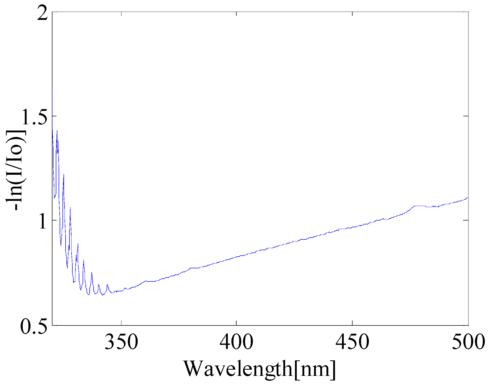
Sensitivity tests aimed at optimizing the CHOCHO retrieval parameters were performed as described in [6]. The simulated spectrum was generated by SCIATRAN, with a spectral range of 365–460 nm, a spectral grid of 0.04 nm and resampling to 0.2 nm, a solar zenith angle of 41°, a surface reflectance of 0.03, and an initial CHOCHO SCD of 3 × 10¹⁵ molec/cm2; however, the rotational Raman scattering of atmospheric N2 and O2 molecules was not considered. Figure 3 shows the logarithm of the ratio of the synthetic spectrum to the solar reference spectrum [30].
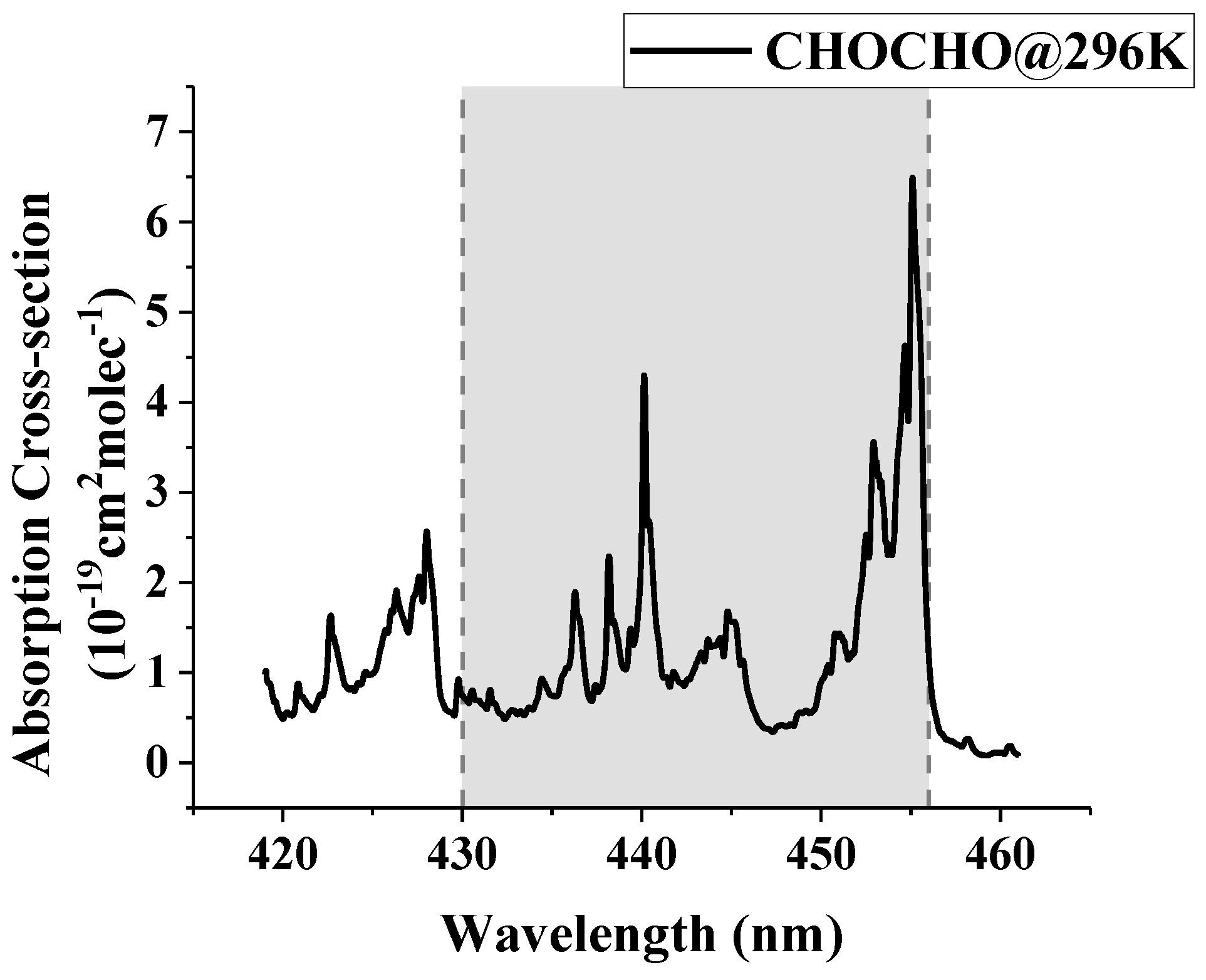
The sensitivity of CHOCHO retrieval depends on the fitting order, fitting window, absorption cross-sections of different NO2 temperatures and interference of NO2 concentrations. Figure 4 shows that glyoxal SCDs are sensitive to the fitting parameter settings. Figure 4a–c show the CHOCHO SCDs retrieved from the synthetic spectrum for wavelength intervals with starting limits of 420–436 nm and ending limits of 444–460 nm. Absorption cross-sections (ACS) of CHOCHO [13] [296 K] and the interfering species NO2 [31] [220 K, 294 K], O3 [32] [223 K], H2O vapor [33,34], and O4 [35] are included in the fitting process, and the solar spectrum from Chance et al. [30] is used as the reference spectrum. All synthetic spectra, reference solar spectra and ACSs are degraded to the OMI resolution through convolution. Consistent with a previous study, which proved that the results are similar for polynomial orders 3 and 4 [6], we find that the SCDs retrieved with polynomial orders 3 and 5 show nonphysical negative values and larger variabilities for some fitting intervals. Therefore, order 4 is used for the sensitivity tests in d–f, and Figure 4b is used as the reference scene for d–f. The NO2 cross-section having different temperatures (i.e., 294 K) is proven to significantly affect the retrieval results, which can be seen in Figure 4d. Without the NO2 cross-section at 294 K, the relative change () with respect to Figure 4b can be seen in Figure 4e. This change is drastic, especially for starting wavelengths below 428 nm and ending wavelengths below 448 nm, which correspond to the wavelength regions where the absorption of glyoxal is weaker than the strong absorption of NO2. To decorrelate the NO2 and CHOCHO absorption features, the NO2 SCD was fixed to a constant 2 × 10¹⁶ molec/cm2, and the signals introduced by NO2 were subtracted from the differential spectrum in Figure 4e. Then, the SCD was fitted without the NO2 cross-section at 294 K. The sensitivity analysis results show that the relative differences of Figure 4f with respect to Figure 4b are within ±10%. The inversion result of CHOCHO is relatively small when the ending wavelength is less than 448 nm and becomes larger when the end wavelength is greater than 448 nm. To accurately test the effects of the temporal-spatial distribution of NO2 on glyoxal retrieval, a detailed comparative analysis based on actual OMI observations is conducted in Section 4 Based on the sensitivity analysis, the fitting window selected in this study is shown in Figure 5. In the following, we use a fitting window of 430–458 nm. This wavelength range covers the strong CHOCHO absorption bands. The fitting parameters used in this paper and in other glyoxal datasets are listed in Table 1.
3.2. Air Mass Factor Computation
SCD depends on the observation geometry, which determines the photon path. An AMF is used to convert SCD into total vertical columns. The AMF is defined as the ratio of the slant column to the vertical column. A geometric AMF () can be defined as , which is a function of solar zenith angle and of satellite viewing angle in the absence of atmospheric scattering. In the actual atmosphere, the AMF also depends on the trace gas profile, air pressure, surface albedo, and aerosol profiles. In this work, the AMFs are calculated by SCIATRAN [36,37]. The typical glyoxal profiles are assumed as described in Wittrock et al. [14], with the maximum values concentrated near the ground, and the values decrease exponentially with height.
AMF is sensitive to the vertical distribution of atmospheric species, and a more sophisticated calculation of HCHO AMF and NO2 includes the effects of clouds [38,39] and aerosols [40,41]. Cloud and aerosol corrections are not included in this work; only pixels with cloud fractions less than 0.2 are available in the glyoxal retrieval. Lorente et al. [42] suggests that the AMF structural uncertainty is 42% over polluted regions and 31% over unpolluted regions, and AMF improvement is needed in the future but is beyond the scope of the present study.
4. Results
4.1. The OMI-CAS Glyoxal Retrieval
In this section, an example of the algorithm applied to the OMI spectrum measured on 26 July 2005 is provided. In this work, the daily mean value of the earthshine spectrum with a cloud fraction of less than 0.2 in the Pacific region [Lat. 20°N–50°N; Long. 160°N–220°N] is used as a reference spectrum. Compared with using the solar irradiance as the reference spectrum, this method can avoid stripe offset of the OMI cross-track position in the SCD retrieval. Hence, a destriping correction is unnecessary. This method was most recently used for NO2, SO2 and HCHO retrievals from the OMI and the TROPOspheric Monitoring Instrument (TROPOMI) [39,47]. With regard to the latitudinal gradient of stratospheric NO2 and other absorbers introduced by the reference, we perform a zonal reference sector correction as described by De Smedt et al. [38]. The latitudinal dependency of the offset-corrected CHOCHO slant columns is modeled by a polynomial for the entire reference sector.
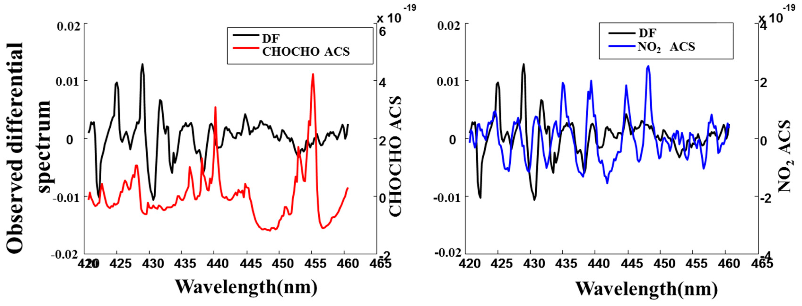
The differential ACSs of NO2 and CHOCHO are coupled, and the correlation between the differential spectral structure and the NO2 differential ACS is better than that with CHOCHO, as shown in Figure 6. On the other hand, eastern China is a globally high region of NO2, and the spatial distribution of NO2 is highly inhomogeneous. However, the interference of NO2 on glyoxal retrieval remains unclear. To further analyze the effects of the NO2 concentration on glyoxal retrieval, we perform a two-step CHOHCO retrieval: step 1 addresses the prefixed tropospheric NO2 SCD from OMI OMNO2 dataset, and step 2 involves the fitting of CHOCHO slant columns, in which the tropospheric NO2 is fixed to the value determined in step 1 and includes cross-sections of CHOCHO (294 K), NO2 (220 K), O3 (223 K), H2O vapor (280 K), and O4 (293 K) and the Ring cross section calculated by the QDOAS Ring tool.
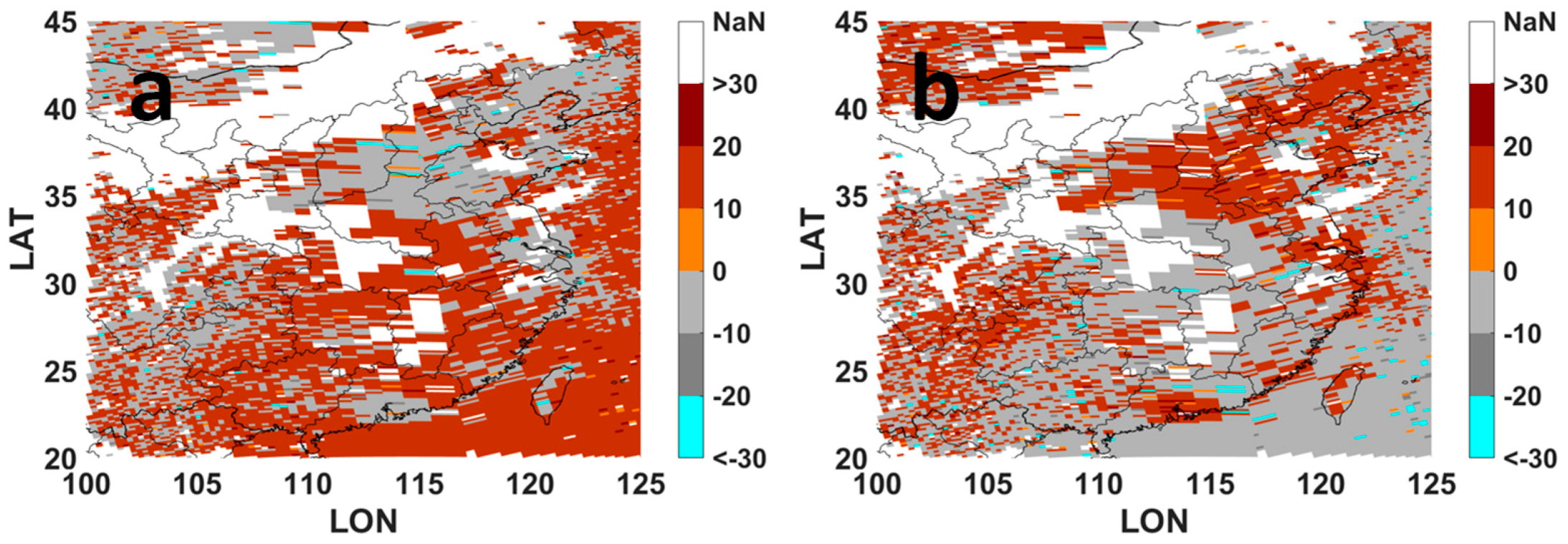
The tropospheric NO2 dataset used in this study changed to 50% and 200% of the original value. We find that the relative difference before and after change, defined as , is not uniform and is related to the spatial distribution of NO2, as presented in Figure 7. A decrease in the NO2 concentration causes an increase in glyoxal, and the change is larger over low-NO2 regions (>30%) than over high-NO2 regions (10%), while doubling the NO2 concentration causes the opposite change. The result shows the retrieved CHOCHO SCD is sensitive to NO2 interference. The differential spectrum can be modified depending on the inhomogeneous temporal-spatial distribution of NO2. Thus, the spatiotemporally varying NO2 abundance can lead to varying in retrieved CHOCHO. Hereafter, we refer to the method of prefixing NO2 during glyoxal retrieval as OMI-CAS.
Figure 8a shows the result of OMI-CAS, and Figure 8b shows the result of OMI-Harvard. The results all show high values in the YRD, Beijing, Tianjin, etc., and OMI-CAS can more clearly represent relative hotspots. The OMI-CAS results compared with the OMI-Harvard dataset as a function of latitude are presented in Figure 8c. The results show that the OMI-CAS has a large variation range between 20°N–25°N. For the SCD > 0, the zonal average of OMI-CAS CHOCHO SCD is 137.96 × 10¹³ molec/cm2 with a standard deviation of 117.22 × 10¹³ molec/cm2, while the standard deviation is almost doubled being 214.89 × 10¹³ molec/cm2 when the negative data considered. Correspondingly, the zonal average of the OMI-Harvard is 119.47 ± 123.80 × 10¹³ molec/cm2 and 24.47 ± 149.35 × 10¹³ molec/cm2 when the negative values excluded and included, respectively. In addition, the fraction of SCD < 0 for OMI-CAS (67.36%) is 23.04% larger than OMI-Harvard (44.32%) in this latitude range, which may be related to the unphysical negative value over the ocean. In contrast, the OMI-CAS results are closer to the OMI-Harvard results over terrestrial China, with the zonal average of 117.53 ± 100.25 × 10¹³ molec/cm2 and 113.42 ± 95.05 × 10¹³ molec/cm2 for the two dataset between 20°N–50°N. Considering that the research area of this paper is mainly continental China and that previous research results show that liquid water does not affect retrieval results over land [21], the resulting sea outliers are not considered in this paper. Figure 9 shows the fitted spectrum compared with the differential spectrum obtained using the SCD retrieval of OMI-CAS.
4.2. Intercomparison with Other Datasets
To evaluate the consistency of OMI-CAS with OMI-Harvard, OMI-IUP and Sciamachy-IUP, we perform a comparison over four typical regions by season in 2005, as shown in Table 2. The seasonal distributions of glyoxal in China of the four datasets are shown in Figure 10. OMI-CAS is shown in the first column. The spatial distributions of the OMI-Harvard, OMI-IUP and Sciamachy-IUP in China are shown in the second, third and fourth columns, respectively. The first to fourth rows represent spring (MAM), summer (JJA), autumn (SON), and winter (DJF). Notably, OMI-IUP and Sciamachy-IUP are systematically lower than OMI-CAS and OMI-Harvard. To plot all datasets in one figure, the glyoxal from IUP is multiplied by a factor of 10 in the following comparison and analysis.
The four datasets exhibit consistent spatial and temporal distributions, and CHOCHO consistently exhibits low winter and high summer characteristics, attributes related to the dependence of VOC emissions on temperature and photochemistry. In terms of spatial distribution, the high values of glyoxal are mainly concentrated in densely populated urban areas, such as the YRD, PRD, and CY areas. The NC region also shows obvious high values in summer, which have strong anthropogenic characteristics.
Figure 11 shows the monthly mean variation in each region. In NC, the maximum value of the OMI-CAS monthly mean occurs in July, with a maximum value of 236.75 ± 41.75 × 10¹³ molec/cm2, and the minimum occurs in both October (200.25 ± 23.80 × 10¹³ molec/cm2) and March (200.75 ± 41.75 × 10¹³ molec/cm2). OMI-Harvard has a similar monthly variation pattern but is higher than OMI-CAS by 8–32 × 1013 molec/cm2, except in July. The largest difference occurs in October. OMI-IUP and Sciamachy-IUP show similar monthly variation patterns, and after October, the concentration of glyoxal shows a significant increasing, accompanied by a larger uncertainty. The increase is also reflected in the OMI-CAS dataset, but the magnitude of OMI-CAS is significantly smaller than that of the other two datasets. In SC, Sciamachy-IUP shows significant differences compared to the other datasets from August to October and should be used with caution. In addition, except for Sciamachy-IUP, the other three datasets showed significantly low values in July over SC, which were related to the influence of the East Asian summer monsoon that contributed to good diffusion conditions in southern China. The OMI-CAS also showed a premonsoon accumulation of glyoxal concentration and a postmonsoon rebound of glyoxal, reaching a maximum in October. This monthly variation feature is also consistent with other gaseous pollutants observed in SC, such as NO2 and HCHO [48] In the YRD region, the variation characteristics of the OMI-CAS showed a maximum in July. After October, the concentration of CHOCHO gradually decreased with decreasing temperature, reaching a minimum in winter. OMI-Harvard is similar to OMI-CAS but higher than OMI-CAS. In the CY area, the characteristics shown by OMI-CAS are similar to those in the YRD.
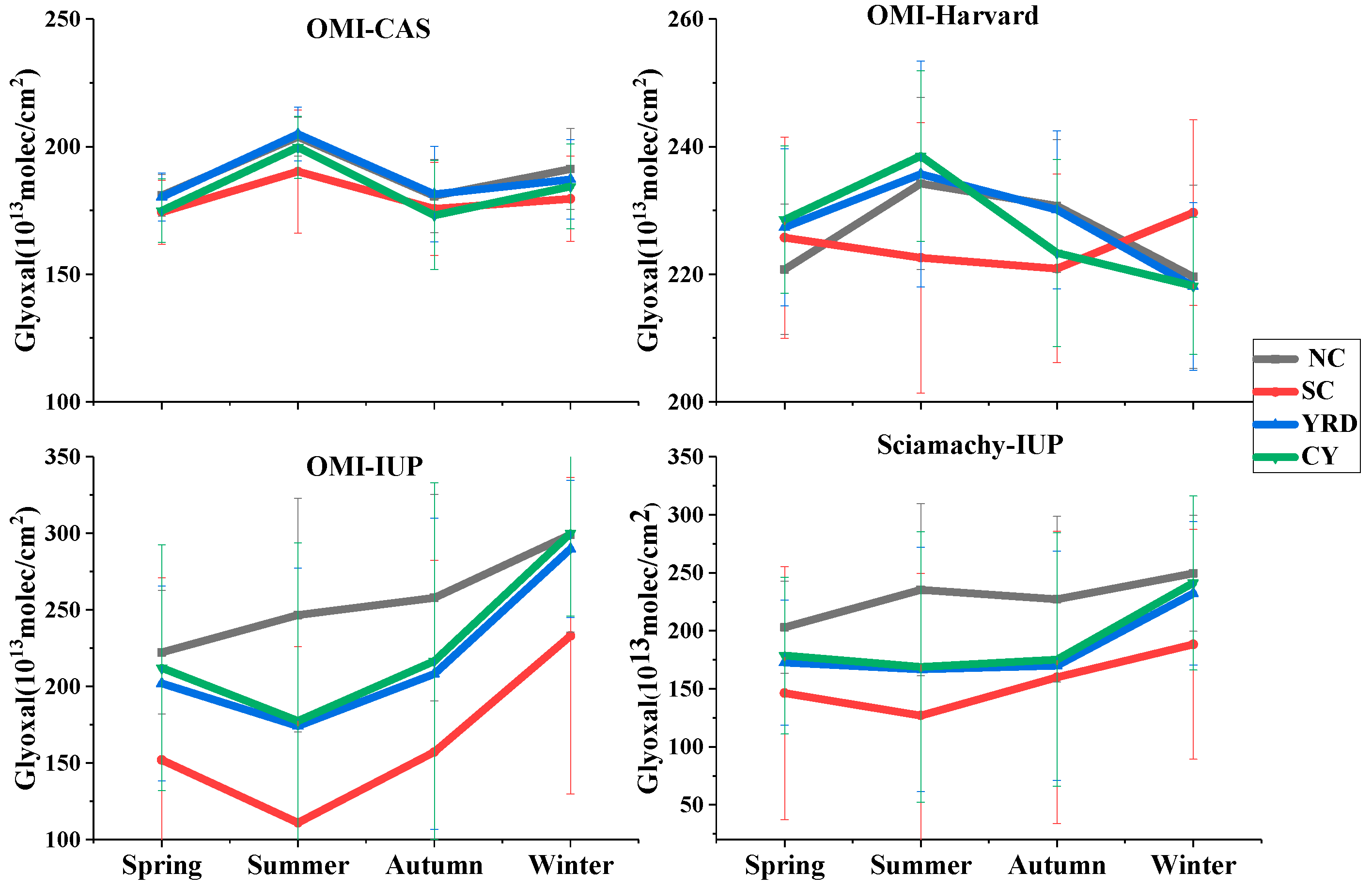
Previous studies suggested that space averaging can reduce the random error of glyoxal [6,10]; therefore, all datasets are resampled to 2.5° × 2.5°. The seasonal variation in glyoxal based on the four datasets is shown in Figure 12. OMI-CAS shows typical seasonal variations in the selected regions, with the maximum observed in summer and the minimum observed in autumn. The winter glyoxal presence is larger than that in spring and autumn and may be introduced by heating in the northern regions or by greater biases in winter. OMI-Harvard also captures the maximum value in summer, except for over SC, where the maximum is observed in winter. Both OMI-IUP and Sciamachy-IUP show the lowest values in summer and the highest values in winter. Notably, the seasonal variation in this study is focused on only the variation pattern because of the large differences in absolute values between OMI-IUP and Sciamachy-IUP compared with OMI-CAS and OMI-Harvard. The large discrepancies between these datasets may be introduced by the parameter settings used in the retrieval.
The correlation analysis results by season over China are shown in Figure 13. The first column represents OMI-CAS and OMI-Harvard; the second column represents OMI-CAS and OMI-IUP; and the third column represents OMI-CAS and Sciamachy-IUP. In spring and winter, OMI-CAS has weak correlations with other three datasets, which may be related to consideration of the tropospheric NO2. In contrast, the correlations between OMI-CAS and OMI-Harvard, OMI-CAS and OMI-IUP, and OMI-CAS and Sciamachy-IUP are best in summer, with R = 0.63, R = 0.67 and R = 0.67, respectively. The correlations between OMI-CAS and OMI-Harvard and OMI-CAS and Sciamachy-IUP in autumn are 0.58 and 0.48, respectively. Table 3 shows the statistical parameters in selected regions in summer and winter. Table S1 shows all seasons. In NC, OMI-Harvard, OMI-IUP and Sciamachy-IUP show the best correlations with OMI-CAS in autumn, with correlations of 0.46, 0.36, and 0.48, respectively, which were higher than those in spring > summer > winter. In SC, the best correlation is seen in summer, and the correlations of the three datasets are 0.79, 0.8 and 0.74, respectively, which were higher than those in autumn (0.63, 0.46, 0.56) > winter (0.45, 0.23, 0.42) > spring (0.08, 0.21, 0.15), respectively. In the YRD region, winter observations showed a significant negative correlation with OMI-CAS. In addition, the autumn correlation was the best (R = 0.58). The CY region showed a significant negative correlation in winter. The correlation between OMI-Harvard and OMI-CAS was the best in autumn (0.62), and the correlation between OMI-IUP and OMI-CAS was the best in spring (0.45). Due to the lack of extensive ground-based observation validations, the correlations between different datasets cannot be used to determine the quality of the dataset. Only the quantitative temporal and spatial comparisons between different datasets can be given to provide users with recommendations.
5. Discussion
In this work, the different Ring effects caused by the use of the daily Pacific earthshine spectrum as a reference have not yet been considered in the CHOCHO retrieval algorithm. We also find that interferences with Fraunhofer features can be partially cancelled out (As show in Figure S1) by using this reference. It should be noted that the interference of stratospheric NO2 is not prefitted due to the target, CHOCHO, being mainly concentrated near the ground; thus, the impact of tropospheric NO2 was given special attention. In addition, the 220 K NO2 cross-section is included in the step 2 of retrieval process, which can account for the signature of stratospheric NO2. Moreover, the absorption of liquid water is not considered in this study due to the main study region is continent.
In NC region, the significant increase of CHOCHO since October may be related to heating in the northern regions during winter, which is consistent with ground measurements in winter, when buildings are heated [49]. This phenomenon is also reflected in the YRD and CY regions for OMI-IUP and Sciamachy-IUP, however, this is inconsistent with our known understanding. The reasons behind this phenomenon need to be studied and may be related to the uncertainty of the algorithm in autumn and winter or to other unknown sources. Particularly, use of the monthly mean value of SCIAMACHY is not recommended in South China due to the obvious difference in the seasonal variation pattern. Similarly, the increases in OMI-IUP and SCIAMACHY in the YRD region since October are not credible and are not recommended for use.
The high correlations of OMI-CAS compared with other datasets in summer and autumn indicate that OMI-CAS can capture glyoxal information. The comparison results show that the correlation between summer and autumn in each region is better than the correlations in spring and winter, which is partly related to the method of prefixing NO2 used in this work.
6. Conclusions
In this work, we present an algorithm for glyoxal retrieval based on OMI measurements. The spatial and temporal variations of NO2 are included in the fitting process. Sensitivity tests on synthetic data indicate that the fitting window of 430–458 nm and the 4th order are appropriate for use in glyoxal retrieval. Moreover, we first tested the differences from using prefixed NO2 and including different NO2 cross-section temperatures, which represent the NO2 interference in the different height layers in fitting of the glyoxal SCD, based on synthetic data and OMI measurements. We find that the difference between the two methods is spatially inhomogeneous. In contrast, upon changing the NO2 test concentration, the result shows strong spatial dependence. The hotspot NO2 regions change less than do the low-NO2 regions when the factor is 0.5, while the change pattern is the opposite when the factor is 2.
The prefixed NO2 method of glyoxal retrieval proposed in this study is performed, and the result is referred to as OMI-CAS. Our results exhibit low winter and high summer characteristics, which indicate that temperature is essential for an enhanced CHOCHO level. The OMI-CAS results intercomparison with the other datasets shows consistent spatial and temporal distribution characteristics overall but shows different monthly and seasonal variations over selected regions during different seasons, as well as different correlation coefficients. In general, the correlation is better in autumn and summer, but the results show almost no correlation or lesser correlations in winter and spring. In the SC region, the best correlations are observed, with the correlations among the four datasets (OMI-CAS and OMI-Harvard, OMI-CAS and OMI-IUP, OMI-CAS and Sciamachy-IUP) being 0.79, 0.8 and 0.74 in summer, respectively, while NC shows the worst correlation in winter, with a negative correlation in the YRD and CY in winter. This discrepancy can be partly attributed to the high and drastic change in NO2 in these regions in winter. Another important reason is the larger biases in winter. According to the comparison results, we propose some recommendations and precautions when using different glyoxal datasets in specific regions and seasons.
Supplementary Materials
The following are available online at https://www.mdpi.com/2072-4292/11/2/137/s1, Figure S1: Irradiance, radiance Pacific and radiance, Table S1: Statistical parameters of comparison, where ‘avg’ represents the mean concentration and ‘std’ represents the standard deviation (unite: 1013 molec/cm2).
Author Contributions
Conceptualization, J.T. and L.C. (Liangfu Chen).; Formal analysis, Y.W.; Methodology, C.Y.; Resources, Z.W.; Validation, L.C. (Liangxiao Cheng).; Writing, review & editing, Y.W.
Funding
This research was funded by the National Key Research and Development Program of China (Grant No. 2017YFB0503901) and the National Natural Science Foundation of China (Grant No. 41771391).
Acknowledgments
We thank all the mission scientists and principal investigators who prepared and provided the OMI datasets used in this study. The authors are grateful to Miller et al. for open access to the OMI glyoxal retrieval results. We are also sincerely grateful to Alvarado et al. for providing the monthly mean glyoxal dataset derived from OMI and SCIAMACHY.
Conflicts of Interest
The authors declare no conflicts of interest.
References
- Strong, J.; Whyatt, J.D.; Metcalfe, S.E.; Derwent, R.G.; Hewitt, C.N. Investigating the impacts of anthropogenic and biogenic VOC emissions and elevated temperatures during the 2003 ozone episode in the UK. Atmos. Environ. 2013, 74, 393–401. [Google Scholar] [CrossRef]
- Sillman, S. The relation between ozone, NOx and hydrocarbons in urban and polluted rural environments. Atmos. Environ. 1999, 33, 1821–1845. [Google Scholar] [CrossRef]
- Li, Y.; Lau, A.K.H.; Fung, J.C.H.; Zheng, J.Y.; Liu, S.C. Importance of NOx control for peak ozone reduction in the Pearl River Delta region. J. Geophys. Res. Atmos. 2013, 118, 9428–9443. [Google Scholar] [CrossRef]
- Han, D.M.; Wang, Z.; Cheng, J.P.; Wang, Q.; Chen, X.J.; Wang, H.L. Volatile organic compounds (VOCs) during non-haze and haze days in Shanghai: characterization and secondary organic aerosol (SOA) formation. Environ. Sci. Pollut. Res. 2017, 24, 18619–18629. [Google Scholar] [CrossRef] [PubMed]
- Wei, W.; Li, Y.; Wang, Y.; Cheng, S.; Wang, L. Characteristics of VOCs during haze and non-haze days in Beijing, China: Concentration, chemical degradation and regional transport impact. Atmos. Environ. 2018, 194, 134–145. [Google Scholar] [CrossRef]
- Alvarado, L.M.A.; Richter, A.; Vrekoussis, M.; Wittrock, F.; Hilboll, A.; Schreier, S.F.; Burrows, J.P. An improved glyoxal retrieval from OMI measurements. Atmos. Meas. Tech. 2014, 7, 5559–5599. [Google Scholar] [CrossRef]
- Zhao, Y.; Mao, P.; Zhou, Y.D.; Yang, Y.; Zhang, J.; Wang, S.K.; Dong, Y.P.; Xie, F.J.; Yu, Y.Y.; Li, W.Q. Improved provincial emission inventory and speciation profiles of anthropogenic non-methane volatile organic compounds: a case study for Jiangsu, China. Atmos. Chem. Phys. 2017, 17, 7733–7756. [Google Scholar] [CrossRef] [Green Version]
- Wei, W.; Wang, S.X.; Chatani, S.; Klimont, Z.; Cofala, J.; Hao, J.M. Emission and speciation of non-methane volatile organic compounds from anthropogenic sources in China. Atmos. Environ. 2008, 42, 4976–4988. [Google Scholar] [CrossRef]
- Fu, T.M.; Jacob, D.J.; Wittrock, F.; Burrows, J.P.; Vrekoussis, M.; Henze, D.K. Global budgets of atmospheric glyoxal and methylglyoxal, and implications for formation of secondary organic aerosols. J. Geophys. Res. Atmos. 2008, 113. [Google Scholar] [CrossRef] [Green Version]
- Miller, C.C.; Jacob, D.J.; Abad, G.G.; Chance, K. Hotspot of glyoxal over the Pearl River delta seen from the OMI satellite instrument: implications for emissions of aromatic hydrocarbons. Atmos. Chem. Phys. 2016, 16, 4631–4639. [Google Scholar] [CrossRef] [Green Version]
- Volkamer, R.; Molina, L.T.; Molina, M.J.; Shirley, T.; Brune, W.H. DOAS measurement of glyoxal as an indicator for fast VOC chemistry in urban air. Geophys. Res. Lett. 2005, 32, 93–114. [Google Scholar] [CrossRef]
- Volkamer, R.; Platt, U.; Wirtz, K. Primary and secondary glyoxal formation from aromatics: Experimental evidence for the bicycloalkyl-radical pathway from benzene, toluene, and p-xylene. J. Phys. Chem. A 2001, 105, 7865–7874. [Google Scholar] [CrossRef]
- Volkamer, R.; Spietz, P.; Burrows, J.; Platt, U. High-resolution absorption cross-section of glyoxal in the UV–vis and IR spectral ranges. J. Photochem. Photobiol. A Chem. 2005, 172, 35–46. [Google Scholar] [CrossRef]
- Wittrock, F.; Richter, A.; Oetjen, H.; Burrows, J.P.; Kanakidou, M.; Myriokefalitakis, S.; Volkamer, R.; Beirle, S.; Platt, U.; Wagner, T. Simultaneous global observations of glyoxal and formaldehyde from space. Geophys. Res. Lett. 2006, 33. [Google Scholar] [CrossRef] [Green Version]
- Vrekoussis, M.; Wittrock, F.; Richter, A.; Burrows, J. GOME-2 observations of oxygenated VOCs: what can we learn from the ratio glyoxal to formaldehyde on a global scale? Atmos. Chem. Phys. 2010, 10, 10145–10160. [Google Scholar] [CrossRef] [Green Version]
- Miller, C.C.; Abad, G.G.; Wang, H.; Liu, X.; Kurosu, T.; Jacob, D.J.; Chance, K. Glyoxal retrieval from the Ozone Monitoring Instrument. Atmos. Meas. Tech. 2014, 7, 3891–3907. [Google Scholar] [CrossRef] [Green Version]
- Liu, Z.; Wang, Y.H.; Vrekoussis, M.; Richter, A.; Wittrock, F.; Burrows, J.P.; Shao, M.; Chang, C.C.; Liu, S.C.; Wang, H.L.; et al. Exploring the missing source of glyoxal (CHOCHO) over China. Geophys. Res. Lett. 2012, 39. [Google Scholar] [CrossRef] [Green Version]
- Cao, H.; Fu, T.M.; Zhang, L.; Henze, D.K.; Miller, C.C.; Lerot, C.; Abad, G.G.; De Smedt, I.; Zhang, Q.; van Roozendael, M.; et al. Adjoint inversion of Chinese non-methane volatile organic compound emissions using space-based observations of formaldehyde and glyoxal. Atmos. Chem. Phys. 2018, 18, 15017–15046. [Google Scholar] [CrossRef]
- Stavrakou, T.; Muller, J.F.; De Smedt, I.; Van Roozendael, M.; Kanakidou, M.; Vrekoussis, M.; Wittrock, F.; Richter, A.; Burrows, J.P. The continental source of glyoxal estimated by the synergistic use of spaceborne measurements and inverse modelling. Atmos. Chem. Phys. 2009, 9, 8431–8446. [Google Scholar] [CrossRef] [Green Version]
- Stavrakou, T.; Muller, J.F.; Bauwens, M.; De Smedt, I.; Lerot, C.; Van Roozendael, M.; Coheur, P.F.; Clerbaux, C.; Boersma, K.F.; van der A, R.; et al. Substantial Underestimation of Post-Harvest Burning Emissions in the North China Plain Revealed by Multi-Species Space Observations. Sci. Rep. 2016, 6. [Google Scholar] [CrossRef]
- Lerot, C.; Stavrakou, T.; De Smedt, I.; Muller, J.F.; Van Roozendael, M. Glyoxal vertical columns from GOME-2 backscattered light measurements and comparisons with a global model. Atmos. Chem. Phys. 2010, 10, 12059–12072. [Google Scholar] [CrossRef] [Green Version]
- Jin, Y.; Andersson, H.; Zhang, S. Air Pollution Control Policies in China: A Retrospective and Prospects. Int. J. Environ. Res. Public Health 2016, 13, 1219. [Google Scholar] [CrossRef]
- Acarreta, J.R.; De Haan, J.F.; Stammes, P. Cloud pressure retrieval using the O2-O2 absorption band at 477 nm. J. Geophys. Res. Atmos. 2004, 109. [Google Scholar] [CrossRef]
- Kleipool, Q.L.; Dobber, M.R.; de Haan, J.F.; Levelt, P.F. Earth surface reflectance climatology from 3 years of OMI data. J. Geophys. Res. Atmos. 2008, 113. [Google Scholar] [CrossRef] [Green Version]
- Krotkov, N.A.; Lamsal, L.N.; Celarier, E.A.; Swartz, W.H.; Marchenko, S.V.; Bucsela, E.J.; Chan, K.L.; Wenig, M.; Zara, M. The version 3 OMI NO2 standard product. Atmos. Meas. Tech. 2017, 10, 3133–3149. [Google Scholar] [CrossRef]
- Marchenko, S.; Krotkov, N.A.; Lamsal, L.N.; Celarier, E.A.; Swartz, W.H.; Bucsela, E.J. Revising the slant column density retrieval of nitrogen dioxide observed by the Ozone Monitoring Instrument. J. Geophys. Res. -Atmos. 2015, 120, 5670–5692. [Google Scholar] [CrossRef] [PubMed] [Green Version]
- Irie, H.; Kanaya, Y.; Takashima, H.; Gleason, J.F.; Wang, Z.F. Characterization of OMI Tropospheric NO2 Measurements in East Asia Based on a Robust Validation Comparison. SOLA 2009, 5, 117–120. [Google Scholar] [CrossRef]
- Irie, H.; Kanaya, Y.; Akimoto, H.; Tanimoto, H.; Wang, Z.; Gleason, J.F.; Bucsela, E.J. Validation of OMI tropospheric NO2 column data using MAX-DOAS measurements deep inside the North China Plain in June 2006: Mount Tai Experiment 2006. Atmos. Chem. Phys. 2008, 8, 6577–6586. [Google Scholar] [CrossRef]
- Lamsal, L.N.; Krotkov, N.A.; Celarier, E.A.; Swartz, W.H.; Pickering, K.E.; Bucsela, E.J.; Gleason, J.F.; Martin, R.V.; Philip, S.; Irie, H.; et al. Evaluation of OMI operational standard NO2 column retrievals using in situ and surface-based NO2 observations. Atmos. Chem. Phys. 2014, 14, 11587–11609. [Google Scholar] [CrossRef]
- Chance, K.; Kurucz, R. An improved high-resolution solar reference spectrum for earth’s atmosphere measurements in the ultraviolet, visible, and near infrared. J. Quant. Spectrosc. Radiat. Transf. 2010, 111, 1289–1295. [Google Scholar] [CrossRef]
- Vandaele, A.C.; Hermans, C.; Simon, P.C.; Carleer, M.; Colin, R.; Fally, S.; Merienne, M.-F.; Jenouvrier, A.; Coquart, B. Measurements of the NO2 absorption cross-section from 42000 cm−1 to 10000 cm−1 (238–1000 nm) at 220 K and 294 K. J. Quant. Spectrosc. Radiat. Transf. 1998, 59, 171–184. [Google Scholar] [CrossRef]
- Malicet, J.; Daumont, D.; Charbonnier, J.; Parisse, C.; Chakir, A.; Brion, J. Ozone UV spectroscopy. II. Absorption cross-sections and temperature dependence. J. Atmos. Chem. 1995, 21, 263–273. [Google Scholar] [CrossRef]
- Gordon, I.E.; Rothman, L.S.; Hill, C.; Kochanov, R.V.; Tan, Y.; Bernath, P.F.; Birk, M.; Boudon, V.; Campargue, A.; Chance, K.V.; et al. The HITRAN2016 molecular spectroscopic database. J. Quant. Spectrosc. Radiat. Transf. 2017, 203, 3–69. [Google Scholar] [CrossRef]
- Rothman, L.S.; Gordon, I.E.; Babikov, Y.; Barbe, A.; Benner, D.C.; Bernath, P.F.; Birk, M.; Bizzocchi, L.; Boudon, V.; Brown, L.R.; et al. The HITRAN2012 molecular spectroscopic database. J. Quant. Spectrosc. Radiat. Transf. 2013, 130, 4–50. [Google Scholar] [CrossRef] [Green Version]
- Thalman, R.; Volkamer, R. Temperature dependent absorption cross-sections of O2–O2 collision pairs between 340 and 630 nm and at atmospherically relevant pressure. Phys. Chem. Chem. Phys. 2013, 15, 15371–15381. [Google Scholar] [CrossRef] [PubMed]
- Rozanov, A.; Rozanov, V.; Buchwitz, M.; Kokhanovsky, A.; Burrows, J.P. SCIATRAN 2.0 – A new radiative transfer model for geophysical applications in the 175–2400 nm spectral region. Advances in Space Research. 2005, 36, 1015–1019. [Google Scholar] [CrossRef]
- Rozanov, V.V.; Rozanov, A.V.; Kokhanovsky, A.A.; Burrows, J.P. Radiative transfer through terrestrial atmosphere and ocean: Software package SCIATRAN. J. Quant. Spectrosc. Radiat. Transf. 2014, 133, 13–71. [Google Scholar] [CrossRef]
- De Smedt, I.; Stavrakou, T.; Hendrick, F.; Danckaert, T.; Vlemmix, T.; Pinardi, G.; Theys, N.; Lerot, C.; Gielen, C.; Vigouroux, C. Diurnal, seasonal and long-term variations of global formaldehyde columns inferred from combined OMI and GOME-2 observations. Atmos. Chem. Phys. 2015, 15, 12241–12300. [Google Scholar] [CrossRef]
- De Smedt, I.; Theys, N.; Yu, H.; Danckaert, T.; Lerot, C.; Compernolle, S.; Van Roozendael, M.; Richter, A.; Hilboll, A.; Peters, E.; et al. Algorithm theoretical baseline for formaldehyde retrievals from S5P TROPOMI and from the QA4ECV project. Atmos. Meas. Tech. 2018, 11, 2395–2426. [Google Scholar] [CrossRef] [Green Version]
- Lin, J.T.; Martin, R.V.; Boersma, K.F.; Sneep, M.; Stammes, P.; Spurr, R.; Wang, P.; Van Roozendael, M.; Clémer, K.; Irie, H. Retrieving tropospheric nitrogen dioxide over China from the Ozone Monitoring Instrument: effects of aerosols, surface reflectance anisotropy and vertical profile of nitrogen dioxide. Atmos. Chem. Phys. 2014, 14, 1441–1461. [Google Scholar] [CrossRef]
- Lin, J.T.; Liu, M.Y.; Xin, J.Y.; Boersma, K.F.; Spurr, R.; Martin, R.; Zhang, Q. Influence of aerosols and surface reflectance on satellite NO2 retrieval: seasonal and spatial characteristics and implications for NOx emission constraints. Atmos. Chem. Phys. 2015, 15, 12653–12714. [Google Scholar] [CrossRef]
- Lorente, A.; Boersma, K.F.; Yu, H.; Dorner, S.; Hilboll, A.; Richter, A.; Liu, M.Y.; Lamsal, L.N.; Barkley, M.; De Smedt, I.; et al. alculation for NO2 and HCHO satellite retrievals. Atmos. Meas. Tech. 2017, 10, 759–782. [Google Scholar] [CrossRef]
- Bogumil, K.; Orphal, J.; Homann, T.; Voigt, S.; Spietz, P.; Fleischmann, O.C.; Vogel, A.; Hartmann, M.; Kromminga, H.; Bovensmann, H. Measurements of molecular absorption spectra with the SCIAMACHY pre-flight model: instrument characterization and reference data for atmospheric remote-sensing in the 230–2380 nm region. J. Photochem. Photobiol. A Chem. 2003, 157, 167–184. [Google Scholar] [CrossRef]
- Vandaele, A.C.; Hermans, C.; Fally, S.; Carleer, M.; Mérienne, M.F.; Jenouvrier, A.; Coquart, B.; Colin, R. Absorption cross-sections of NO2: Simulation of temperature and pressure effects. J. Quant. Spectrosc. Radiat. Transf. 2003, 76, 373–391. [Google Scholar] [CrossRef]
- Chance, K.V.; Spurr, R.J. Ring effect studies: Rayleigh scattering, including molecular parameters for rotational Raman scattering, and the Fraunhofer spectrum. Appl Opt. 1997, 36, 5224–5230. [Google Scholar] [CrossRef]
- Wang, P.; Stammes, P.; van der A, R.; Pinardi, G.; van Roozendael, M. FRESCO+: An improved O2 A-band cloud retrieval algorithm for tropospheric trace gas retrievals. Atmos. Chem. Phys. 2008, 8, 6565–6576. [Google Scholar] [CrossRef]
- Theys, N.; De Smedt, I.; Yu, H.; Danckaert, T.; van Gent, J.; Hormann, C.; Wagner, T.; Hedelt, P.; Bauer, H.; Romahn, F.; et al. Sulfur dioxide retrievals from TROPOMI onboard Sentinel-5 Precursor: algorithm theoretical basis. Atmos. Meas. Tech. 2017, 10, 119–153. [Google Scholar] [CrossRef] [Green Version]
- Wang, Y.; Yu, C.; Tao, J.; Wang, Z.; Si, Y.; Cheng, L.; Wang, H.; Zhu, S.; Chen, L. Spatio-Temporal Characteristics of Tropospheric Ozone and Its Precursors in Guangxi, South China. Atmosphere. 2018, 9, 355. [Google Scholar] [CrossRef]
- Yang, W.Q.; Zhang, Y.L.; Wang, X.M.; Li, S.; Zhu, M.; Yu, Q.Q.; Li, G.H.; Huang, Z.H.; Zhang, H.N.; Wu, Z.F.; et al. Volatile organic compounds at a rural site in Beijing: influence of temporary emission control and wintertime heating. Atmos. Chem. Phys. 2018, 18, 12663–12682. [Google Scholar] [CrossRef]
Figure 1.
The study region.
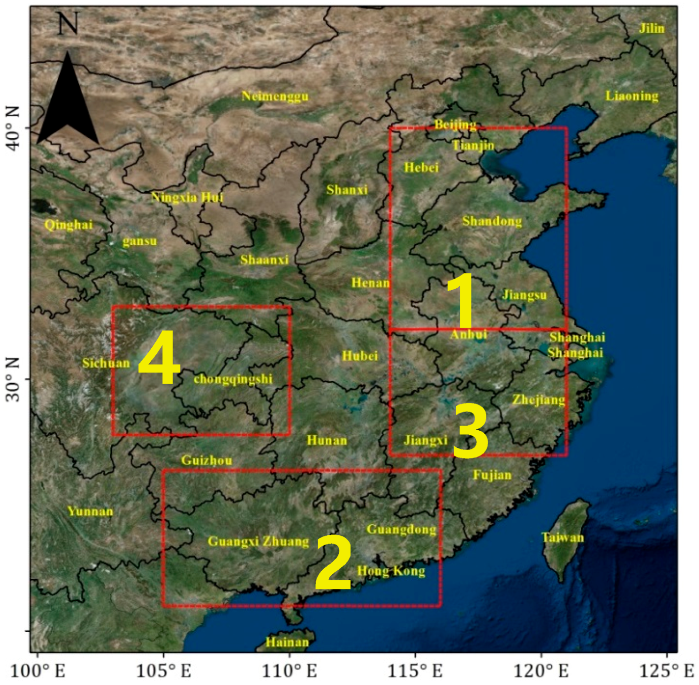
Figure 2.
Absorption intensity of atmospheric components between 300 nm and 500 nm. The slant columns were taken as 1014 molec/cm2 for BrO, 2 × 10¹⁶ molec/cm2 for HCHO, 2 × 10¹⁶ molec/cm2 for NO2, 2 × 1043 molec2/cm5 for O4 and 2 × 10¹⁵ molec/cm2 for CHOCHO.
Figure 2.
Absorption intensity of atmospheric components between 300 nm and 500 nm. The slant columns were taken as 1014 molec/cm2 for BrO, 2 × 10¹⁶ molec/cm2 for HCHO, 2 × 10¹⁶ molec/cm2 for NO2, 2 × 1043 molec2/cm5 for O4 and 2 × 10¹⁵ molec/cm2 for CHOCHO.
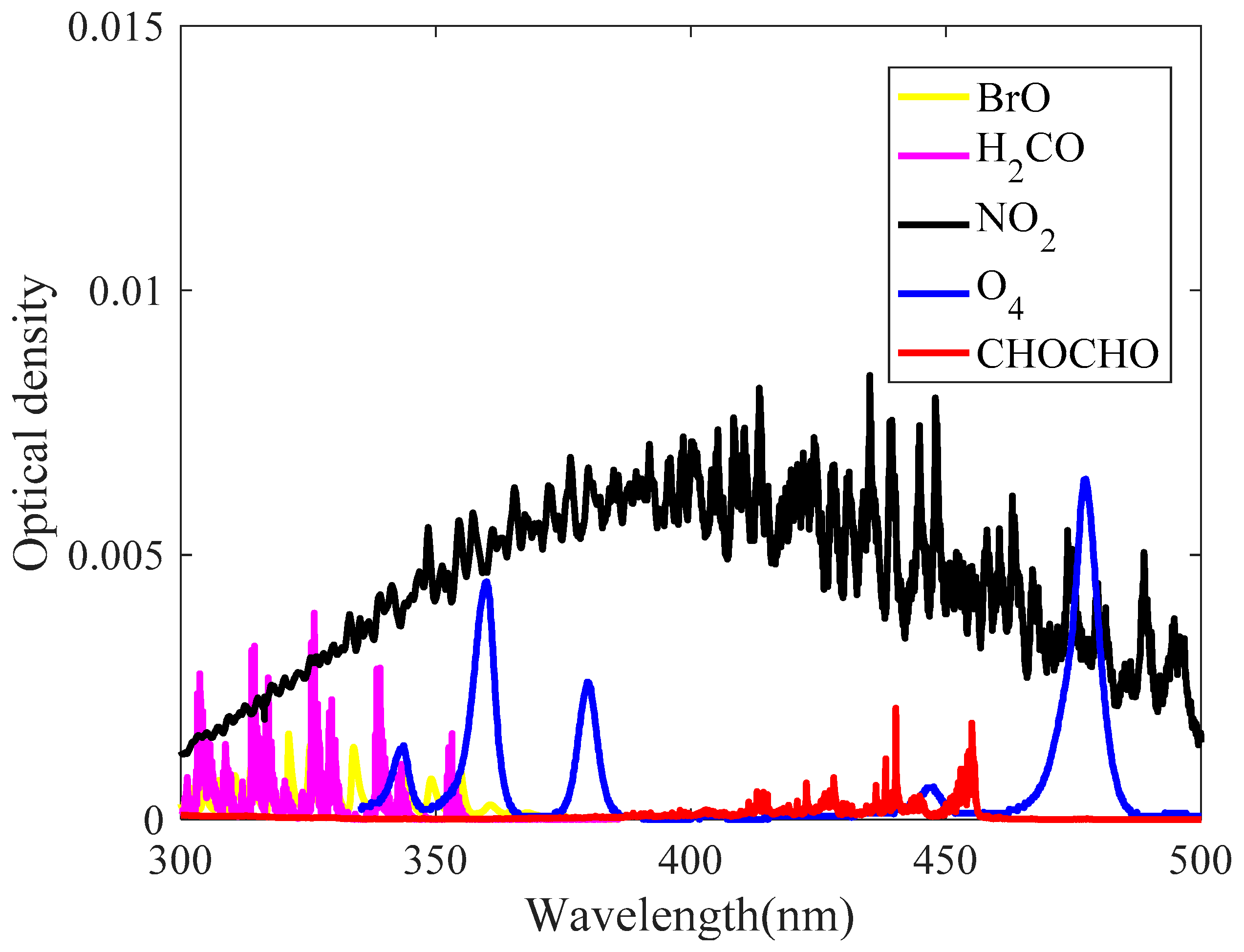
Figure 3.
The logarithm of the ratio of the synthetic spectrum to the solar reference spectrum.

Figure 4.
(a–c) Color mapping of CHOCHO SCD retrieved from a synthetic spectrum for wavelength intervals with starting limits of 420–436 nm, ending limits of 444–460 nm, and polynomial orders of 3, 4 and 5; (d) same as a–c, but without NO2 cross-section in the retrieval; and (e,f) the relative difference between the CHOCHO SCD retrieved from a synthetic spectrum and the SCD in (b).

Figure 5.
The selected fitting interval.

Figure 6.
The differential ACS of NO2 and CHOCHO with respect to the differential spectra (DF). (Left) CHOCHO and differential spectrum; (right) NO2 and differential spectrum.
Figure 6.
The differential ACS of NO2 and CHOCHO with respect to the differential spectra (DF). (Left) CHOCHO and differential spectrum; (right) NO2 and differential spectrum.

Figure 7.
(a) The relative change in the CHOCHO SCD caused by a 50% decrease in NO2 values. (b) The relative change in the CHOCHO SCD caused by a 100% increase in NO2 values.
Figure 7.
(a) The relative change in the CHOCHO SCD caused by a 50% decrease in NO2 values. (b) The relative change in the CHOCHO SCD caused by a 100% increase in NO2 values.

Figure 8.
(a) The results of OMI-CAS. (b) The results from OMI-Harvard. (c) A scatterplot of OMI-CAS and OMI-Harvard as a function of latitude.
Figure 8.
(a) The results of OMI-CAS. (b) The results from OMI-Harvard. (c) A scatterplot of OMI-CAS and OMI-Harvard as a function of latitude.
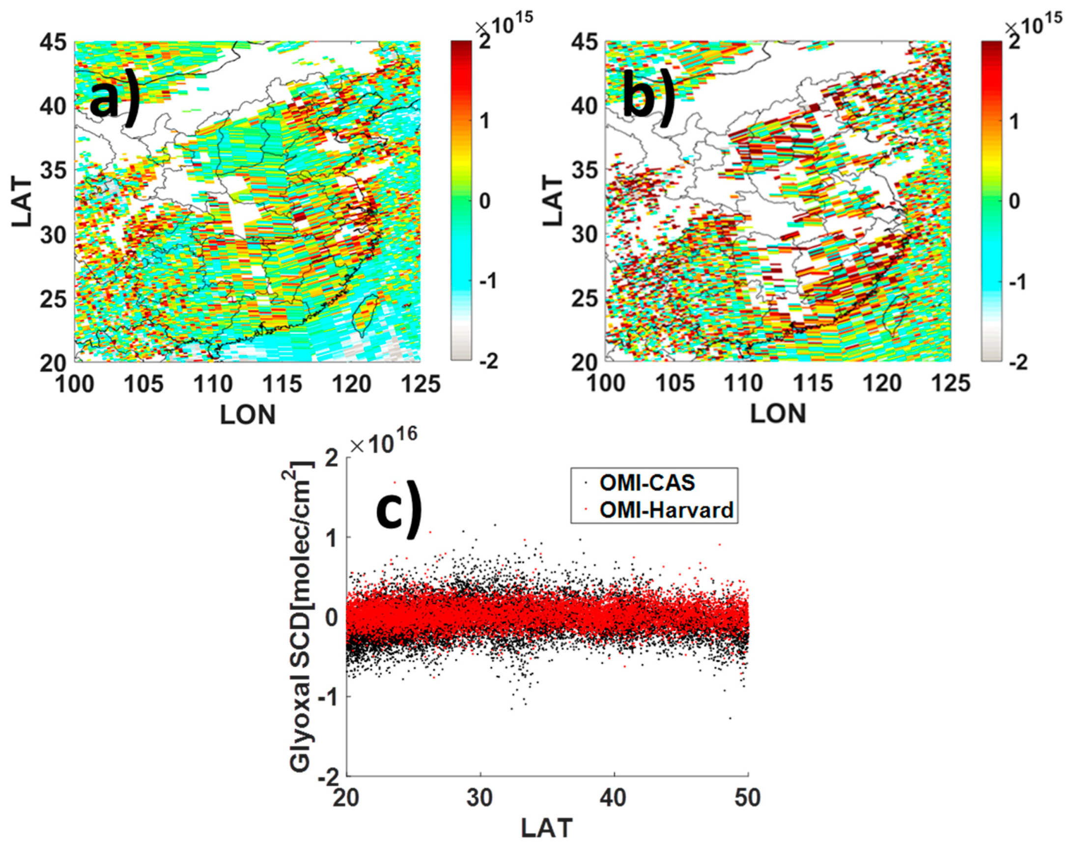
Figure 9.
The fitted spectrum compared with the differential spectrum (DF): (a) with SCDglyoxal = 3.73 × 10¹⁵ molec/cm2; (b) with SCDglyoxal = 2.74 × 10¹⁵ molec/cm2.
Figure 9.
The fitted spectrum compared with the differential spectrum (DF): (a) with SCDglyoxal = 3.73 × 10¹⁵ molec/cm2; (b) with SCDglyoxal = 2.74 × 10¹⁵ molec/cm2.
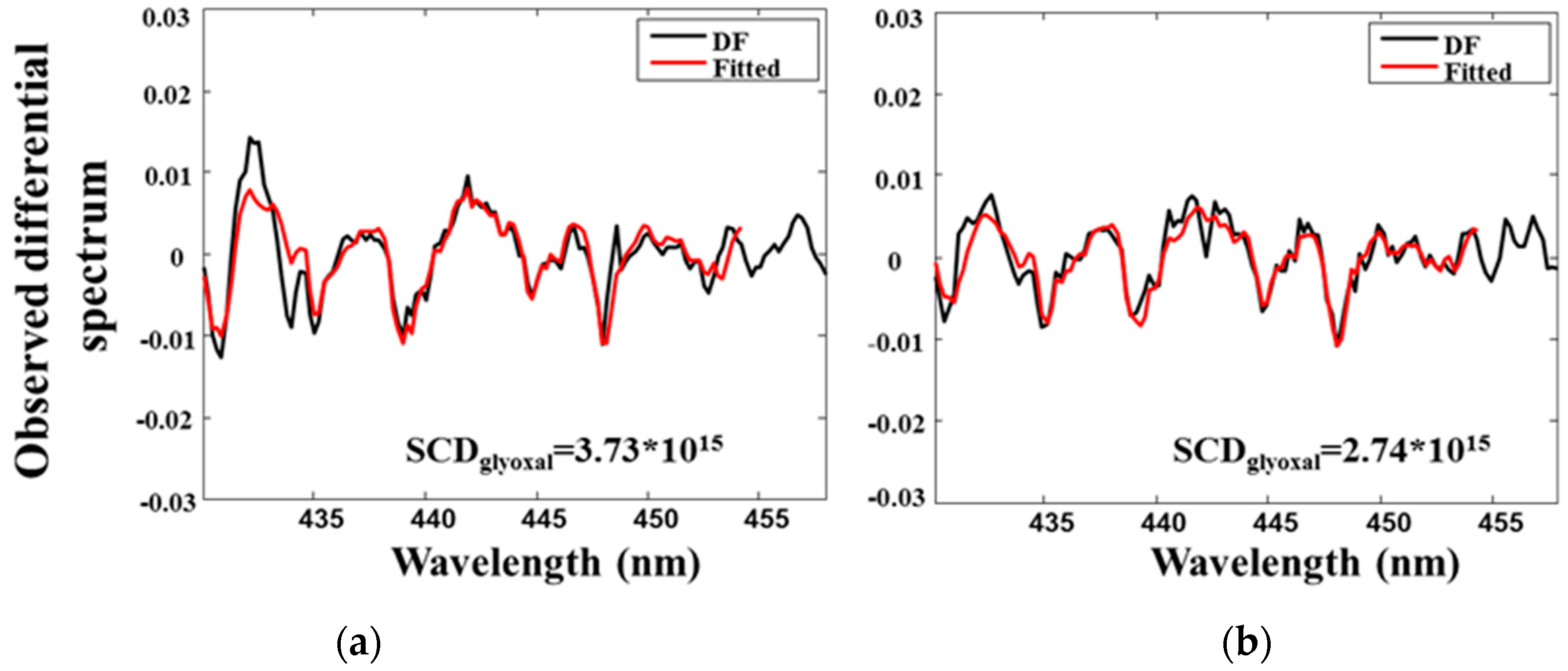
Figure 10.
The seasonal distribution of glyoxal in China in 2005. From left to right: OMI-CAS, OMI-Harvard, OMI-IUP, and Sciamachy-IUP; From top to bottom: spring (MAM), summer (JJA), autumn (SON) and winter (DJF).
Figure 10.
The seasonal distribution of glyoxal in China in 2005. From left to right: OMI-CAS, OMI-Harvard, OMI-IUP, and Sciamachy-IUP; From top to bottom: spring (MAM), summer (JJA), autumn (SON) and winter (DJF).

Figure 11.
Glyoxal monthly mean variations in the selected regions.
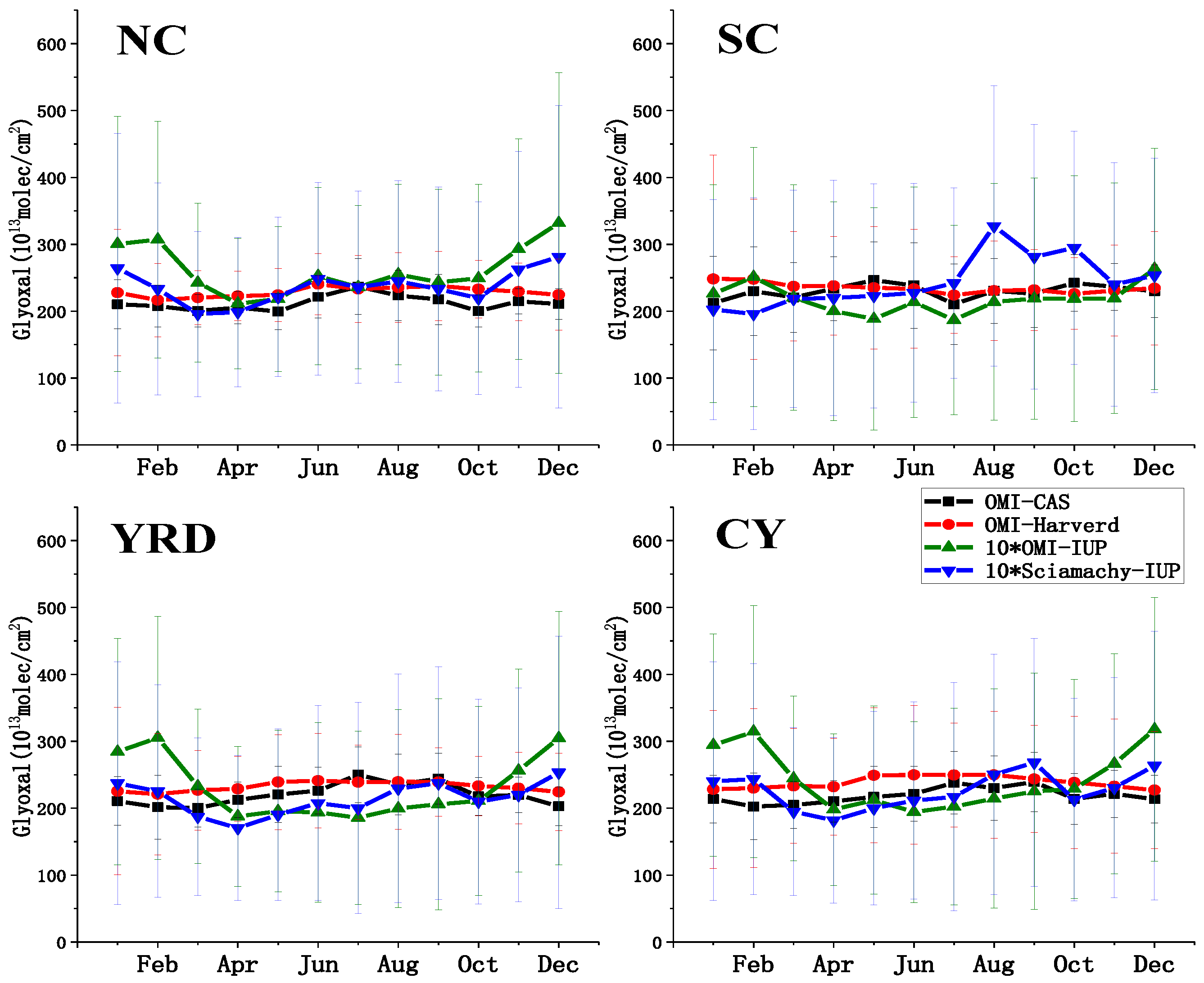
Figure 12.
Seasonal variations of glyoxal based on the four datasets.

Figure 13.
OMI-CAS glyoxal correlation with different datasets over China (Left: OMI-CAS and OMI-Harvard; Middle: OMI-CAS and OMI-IUP; Right: OMI-CAS and Sciamachy-IUP; Resolution = 2.5° × 2.5°; Top to bottom: spring (MAM), summer (JJA), autumn (SON), winter (DJF)).
Figure 13.
OMI-CAS glyoxal correlation with different datasets over China (Left: OMI-CAS and OMI-Harvard; Middle: OMI-CAS and OMI-IUP; Right: OMI-CAS and Sciamachy-IUP; Resolution = 2.5° × 2.5°; Top to bottom: spring (MAM), summer (JJA), autumn (SON), winter (DJF)).


Table 1.
CHOCHO retrieval parameter settings.
| OMI-CAS | OMI-Harvard | OMI-IUP | Sciamachy-IUP | ||
|---|---|---|---|---|---|
| Fitting window | 430–458 nm | w1: liquid water 385–470 nm | w1: liquid water 410–495 nm | The same as OMI-IUP | |
| w2: glyoxal 435–461 nm | w2: glyoxal 433–458 nm | ||||
| Reference spectrum I0 | Pacific region(daily) | Monthly mean solar irradiance | Pacific region (daily) | ||
| Polynomial | 4th-order | Direct spectrum fitting approach | 3rd-order | 4th-order | |
| Included cross-sections | CHOCHO | √ (296 K) | √ (296 K) | √ (296 K) | √ (296 K) |
| O3 [43] | √ (223 K) | √ (243 K) | √ (223 K) | √ (223 K) | |
| NO2 [44] | √ 1 | √ (220, 294 K) | √ (220, 294 K) | √ (220, 294 K) | |
| O4 | √ (293 K) | √ (293 K) | √ (293 K) | √ (293 K) | |
| H2O | √ (280 K) | √ (280 K) | √ (280 K) | √ (280 K) | |
| H2O (liquid) | × | √ (295 K) | √ (295 K) | × | |
| Ring Effect | calculates by QDOAS Ring tool | uses the Ring spectrum of Chance and Spurr [45] | accounts for both rotational and vibrational Raman scattering [14] | ||
| Cloud Fraction | OMCLDO2 [23] | FRESCO+ [46] | |||
| Destriping correction | × | 5-day mean of the SCD retrieved over the Sahara (20°–30°N, 10°W–30°E) | SCD over selected region (30°N–30°S; 160°E−140°W) | × | |
NO2 are fixed in the glyoxal, NO2 (294 k) is not include in the fitted.
Table 2.
Regions selected for Figure 1.
Table 2.
Regions selected for Figure 1.
| Name | Latitude [°] | Longitude [°] | Abbreviation | |
|---|---|---|---|---|
| 1 | North China | [35 40] | [114 121] | NC |
| 2 | South China | [21 26.4] | [105 116] | SC |
| 3 | Yangtze River Delta | [27 35] | [114 121] | YRD |
| 4 | Sichuan and Chongqing region | [27.8 32.9] | [103 110] | CY |
Table 3.
Statistical parameters of comparison, where ‘avg’ represents the mean concentration and ‘std’ represents the standard deviation (unite: 1013 molec/cm2).
Table 3.
Statistical parameters of comparison, where ‘avg’ represents the mean concentration and ‘std’ represents the standard deviation (unite: 1013 molec/cm2).
| OMI-CAS | OMI-Harvard | OMI-IUP | Sciamachy-IUP*10 | ||||||
|---|---|---|---|---|---|---|---|---|---|
| Summer | Autumn | Summer | Autumn | Summer | Autumn | Summer | Autumn | ||
| NC | mean | 203.83 | 180.62 | 234.23 | 230.70 | 246.66 | 258.00 | 235.32 | 227.26 |
| std | 7.61 | 14.30 | 13.52 | 10.40 | 76.37 | 67.33 | 74.20 | 71.41 | |
| R | - | - | 0.09 | 0.46 | 0.12 | 0.36 | 0.14 | 0.48 | |
| slope | - | - | 0.05 | 0.62 | 0.01 | 0.08 | 0.02 | 0.11 | |
| intercept | - | - | 192.25 | 36.95 | 199.32 | 154.45 | 197.31 | 149.44 | |
| SC | mean | 190.24 | 175.67 | 222.58 | 220.91 | 111.04 | 157.26 | 126.97 | 159.87 |
| std | 24.23 | 18.26 | 21.20 | 14.78 | 114.94 | 125.03 | 122.68 | 125.82 | |
| R | - | - | 0.79 | 0.63 | 0.80 | 0.46 | 0.74 | 0.56 | |
| slope | - | - | 0.90 | 0.72 | 0.22 | 0.11 | 0.19 | 0.11 | |
| intercept | - | - | −10.744 | 16.89 | 127.40 | 140.34 | 139.28 | 141.71 | |
| YRD | mean | 204.93 | 181.39 | 235.71 | 230.10 | 174.24 | 208.27 | 166.80 | 169.96 |
| std | 10.48 | 18.72 | 17.70 | 12.41 | 103.18 | 101.69 | 105.31 | 98.73 | |
| R | - | - | 0.31 | 0.34 | 0.22 | 0.32 | 0.32 | 0.58 | |
| slope | - | - | 0.18 | 0.52 | 0.03 | 0.09 | 0.05 | 0.14 | |
| intercept | - | - | 161.92 | 61.86 | 194.29 | 148.25 | 186.85 | 135.05 | |
| CY | mean | 199.73 | 173.15 | 238.51 | 223.34 | 177.57 | 216.68 | 168.88 | 175.17 |
| std | 12.10 | 21.35 | 13.38 | 14.70 | 116.28 | 116.48 | 116.45 | 109.09 | |
| R | - | - | 0.35 | 0.62 | 0.42 | 0.29 | 0.49 | 0.52 | |
| slope | - | - | 0.32 | 0.91 | 0.08 | 0.11 | 0.09 | 0.15 | |
| intercept | - | - | 123.53 | −28.93 | 171.84 | 132.85 | 170.27 | 126.60 | |
© 2019 by the authors. Licensee MDPI, Basel, Switzerland. This article is an open access article distributed under the terms and conditions of the Creative Commons Attribution (CC BY) license (http://creativecommons.org/licenses/by/4.0/).
Share and Cite
MDPI and ACS Style
Wang, Y.; Tao, J.; Cheng, L.; Yu, C.; Wang, Z.; Chen, L. A Retrieval of Glyoxal from OMI over China: Investigation of the Effects of Tropospheric NO2. Remote Sens. 2019, 11, 137. https://doi.org/10.3390/rs11020137
AMA Style
Wang Y, Tao J, Cheng L, Yu C, Wang Z, Chen L. A Retrieval of Glyoxal from OMI over China: Investigation of the Effects of Tropospheric NO2. Remote Sensing. 2019; 11(2):137. https://doi.org/10.3390/rs11020137
Chicago/Turabian StyleWang, Yapeng, Jinhua Tao, Liangxiao Cheng, Chao Yu, Zifeng Wang, and Liangfu Chen. 2019. "A Retrieval of Glyoxal from OMI over China: Investigation of the Effects of Tropospheric NO2" Remote Sensing 11, no. 2: 137. https://doi.org/10.3390/rs11020137
Note that from the first issue of 2016, this journal uses article numbers instead of page numbers. See further details here.