Urban Tomographic Imaging Using Polarimetric SAR Data


Dipartimento di Ingegneria, Università Degli Studi di Napoli “Parthenope”, 80133 Napoli NA, Italy
*
Author to whom correspondence should be addressed.
Remote Sens. 2019, 11(2), 132; https://doi.org/10.3390/rs11020132
Submission received: 30 November 2018
/
Revised: 27 December 2018
/
Accepted: 8 January 2019
/
Published: 11 January 2019
(This article belongs to the Special Issue Urban Deformation Monitoring using Persistent Scatterer Interferometry and SAR tomography)
Abstract
:In this paper, we investigate the potential of polarimetric Synthetic Aperture Radar (SAR) tomography (Pol-TomoSAR) in urban applications. TomoSAR exploits the amplitude and phase of the received data and offers the possibility to resolve multiple scatters lying in the same range–azimuth resolution cell. In urban environments, this issue is very important since layover causes multiple coherent scatterers to be mapped in the same range–azimuth image pixel. To achieve reliable and accurate results, TomoSAR requires a large number of multi-baseline acquisitions which, for satellite-borne SAR systems, are collected with long time intervals. Then, accurate tomographic reconstructions would require multiple scatterers to remain stable between all the acquisitions. In this paper, an extension of a generalized likelihood ratio test (GLRT)-based tomographic approach, denoted as Fast-Sup-GLRT, to the polarimetric data case is introduced, with the purpose of investigating if, in urban applications, the use of polarimetric channels allows for reduction of the number of baselines required to achieve a given scatterer’s detection performance. The results presented show that the use of dual polarization data allows the proposed detector to work in an equivalent or better way than use of a double number of independent single polarization channels.
1. Introduction
Over the past few years, Synthetic Aperture Radar (SAR) sensors have rapidly advanced, offering multi-channel operation (polarimetry, multifrequency), improved range and azimuth resolution, and frequent revisiting of the same area (time series). A new class of SAR satellites, such as TerraSAR-X and TanDEM-X (X-band), COSMO-SkyMed (X-band), as well as Radarsat-2 (C-band), are providing images with resolution in the meter regime, and dual or full polarimetric SAR acquisition modes. In particular, the future second generation of COSMO-SkyMed will have full polarimetric SAR acquisition modes [1,2].
In polarimetric SAR (PolSAR) systems, the antennas for transmitting and receiving electromagnetic waves are configured in different polarization states. Thus, the scattering properties of the observed targets can be revealed in the alternative polarimetric combinations, providing more information compared to single polarization systems [3]. Of course, the price to pay for having enhanced polarization characteristics is a more complex sensor design and the demand for more image storage space.
PolSAR has many applications in many fields, including agricultural areas classification, oceanography (surface currents and wind field retrieval), forest monitoring and classification, disaster monitoring, and target recognition/classification [3]. PolSAR decomposition methods exploiting fully polarimetric data have been successfully applied to map vegetated areas by separating single bounce, double bounce, and volume scattering mechanisms [3]. For urban areas, the polarimetric scattering mechanisms are more complicated with respect to natural areas, due to the high variability of materials, and forms and sizes of the objects laying in the observed ground scene. Different approaches using fully polarimetric SAR data have been recently proposed [4]. In [4] the double bounce scattering form, the dihedral structure formed by the wall and the ground of a building, or the single bounce scattering from the roof or the wall, is considered, for a deterministic extraction of urban areas. However, the rotated dihedral scattering of a building, with a large orientation angle with respect to the radar look direction, results in a strong cross polarization component that can be misdetected as vegetation volume scattering [5].
An alternative approach for urban area monitoring is SAR tomography (TomoSAR). TomoSAR [6] extends the conventional two-dimensional SAR imaging principle to three dimensions by forming an additional synthetic aperture in elevation, using a stack of multi-baseline interferometric images. A fully 3-D scene reflectivity profile along azimuth, range, and elevation is provided. The use of TomoSAR techniques allows the identification of multiple scatterers in the same range–azimuth resolution cell [7]. Tomographic processing can be performed by Fourier-based techniques, beamforming, or spectral methods, such as Capon, MUSIC [8], and the more recent CS (compressive sensing) [9,10,11]. In CS-based approaches, TomoSAR is performed as the recovering of a sparse signal by a convex l1 norm minimization [12] while, in [9,10], the CS approach can improve resolution in elevation and, in [11], the proposed method achieves super-resolution reconstruction, both for range and elevation.
Regardless of whichever imaging technique is adopted for the elevation reflectivity profile focusing, the discrimination between reliable scatterers and false alarms is not an easy task. Since tomographic synthetic aperture in the elevation direction is sampled sparsely, and not regularly and densely, as requested by a Fourier approach, ambiguities and masking problems from anomalous sidelobes may arise. This event, in addition to the presence of noise, produces false alarms. In [13,14,15,16,17], this problem has been addressed on the basis of a generalized likelihood ratio test (GLRT), that allows evaluation of the detection performance in terms of probability of detection achievable with a fixed probability of false alarm. The authors proposed a GLRT detector [14,15,16] that searches for the signal support (i.e., the positions of the significant samples in the unknown vector) that best matches the data. This statistical test is based on a non-linear maximization for detecting single and double scatterers with an assigned probability of false alarm. The elevation of the detected scatterers is then estimated on the basis of their position in the unknown vector.
A problem to be considered is that the performance of the GLRT detector becomes poor when the number of acquisitions or the scatterer coherence decrease [15]. A possible way for increasing the number of acquisition, while keeping the scatterer coherence high, is to exploit polarimetric systems.
Many applications of polarimetric TomoSAR (Pol-TomoSAR) are related to forest vertical structure recovering [18,19,20,21]. The vertical position of the scatterers in a forest, as well as a physical interpretation of the profile, has been shown to be more feasible by coupling polarimetric and multi-baseline information.
Recently, in polarimetric SAR tomography over urban areas [22], different spectral estimation techniques have been extended to the case of multi-pass SAR data acquired with different polarization channels, and a building layover has been studied to compare single and full polarization beamforming, Capon, and MUSIC. There are two drawbacks of these techniques: one is the use of a boxcar filter for the covariance matrix estimation, that reduces resolution in range and azimuth; the second is related to the absence of an approach for identifying multiple scatterers, which are recovered by visual inspection of the reconstructed 3-D reflectivity profile. In [23], a CS approach for polarimetric SAR tomography is proposed. In particular, it exploits the inter-signal structural correlations between neighboring pixels, as well as between polarimetric channels, applying distributed compressed sensing (DCS) theory. In this approach, the elimination of the artifacts and CS algorithm instability can be an issue.
The aim of this paper is to exploit the information given by a polarimetric SAR system, in order to detect reliable single and double scatterers in urban areas by using a reduced number of baselines with respect to the single polarization case. In particular, we will extend the signal model defined in [15], in order to take into account the different polarization channels. Following the approach presented in [22,23], we can suppose that all unknown reflectivity signals throughout polarimetric channels share, approximately, the same sparse support in the space domain, but have different nonzero coefficients. The proposed approach will be validated on dual polarimetric SAR real data.
2. Signal Model
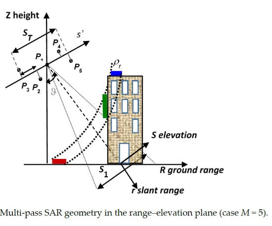
In Figure 1, the multi-pass SAR geometry in the range–elevation plane in a typical urban environment is shown. The three highlighted contributions of the backscattered signal are at the same distance from the platform, and will interfere in the same range–azimuth cell (azimuth axis is orthogonal to the plane). The three contributions come from the ground, the façade, and the roof of the building. In this particular case, the backscattered reflectivity elevation profile, γ, will exhibit only three samples different from zero. Moreover, γ can be assumed to be sparse with, at most, Kmax samples different from zero, typically with Kmax = 2. In order to estimate the reflectivity function γ, a stack of M range–azimuth-focused images is collected. The single channel k-th image, acquired along the orbit with the orthogonal baseline (see Figure 1), in a fixed pixel, is given by the integral superposition of the contributions of all the scatterers lying in the corresponding range–azimuth resolution cell, and located at different elevation coordinates s. A discrete estimate of γ can be found by ideally discretizing the integral operator.
We can denote, with γ, the N × 1 column vector whose elements are the samples of the reflectivity at a fixed range and azimuth position, so the sampled received signal is related to γ by
where u is an M × 1 observations column vector, w is an M × 1 column vector representing noise and clutter, and Φ is an M × N measurement matrix related to the acquisition geometry, whose generic element with index kl is given by
with λ the operating wavelength, and R0 the distance between the center of the scene and a reference antenna position.
We note that in the signal model (1), we have assumed the absence of any phase miscalibration, the compensation of atmospheric delay, and the absence of temporal and thermal deformations.
When considering the fully polarimetric case, the received signal can be modeled as 3M × 1 observations column vector , and one M × 1 vector for each polarimetric channel (HH, HV, VV). We can also assume that is a 3N × 1 reflectivity column vector and that, throughout, the three polarimetric channels share the same sparse support, as we are expecting backscatter from the same structure within a range–azimuth cell [22,23]. Under the above assumptions, we can extend model (1) to a fully polarimetric case:
where w’ is an 3M × 1 column vector representing noise and clutter, and Φ′ is a 3M × 3N block diagonal measurement matrix related to the acquisition geometry, and given by
where 0 is an all-zero M × N matrix.
Note that model (3) can be easily particularized to the dual polarization case by considering only the two available channels in the definition of the vectors u′ and γ′, and only two of the three blocks Φ on the diagonal of Φ′, defined by (4).
3. Pol-TomoSAR Technique
TomoSAR techniques aims at the estimation of by inverting the model (3). The inversion of (3) is ill-posed, since the M acquisitions are not uniformly spaced and usually M < qN, with q being the number of polarization channels. Then, false alarms can appear in the reconstructed profiles, heavily affecting the accuracy of the results. The selection of the most reliable scatterers in each range–azimuth cell can be set as a statistical detection problem assuming, as a selection criterion, the probability of false alarm (PFA) is achievable using a proper statistical test.
In this paper, the polarimetric reflectivity profile is estimated using a GLRT method [24], denoted as Fast-Sup-GLRT [15], which is an approximated and faster version of the GLRT proposed in [14]. Assuming that the maximum number of scatterers in each resolution cell is Kmax, the vector can be assumed to be sparse with, at most, qKmax significant samples, and the detection problem can be formulated as in [14,15], in the terms of the following Kmax + 1 statistical hypothesis:
assuming that urban environment Kmax is typically set as equal to two.
Hi: presence of i scatterers in each channel, with i = 0, …, Kmax,
The noise vector w can be assumed as a circularly symmetric complex Gaussian vector. Consequently, assuming deterministic scatterers, u is a circularly symmetric Gaussian random vector. Exploiting these statistical assumptions, the Fast-Sup-GLRT detector [15] can be extended to the polarimetric model (3). Then, at each step i, the following binary test is applied:
where is the estimated support of cardinality i − 1 of each of the polarimetric vectors , with ab ∈ {HH, HV, VV}, supposed to be (i − 1)-sparse, , with the matrix obtained by substituting in the definition (4) the matrix in the place of Φ, where is obtained from Φ by extracting the i – 1 columns of index . Moreover, is the estimated support of cardinality Kmax of . Each support is estimated by sequentially minimizing the term over k supports of cardinality one [15]. All thresholds can be numerically evaluated by means of Monte Carlo simulations. Assuming Kmax = 2, the two thresholds will be evaluated in such a way to obtain the assigned probabilities of false alarm and false detection, respectively, and .
4. Results and Discussion
In this section, results of the Fast-Sup-GLRT detector (5), that takes into account polarization channels on real data, are presented and compared with the case of only one channel. In processing real data, we limit the search to two targets (Kmax = 2) per resolution cell.
We consider a total of 39 Spotlight TerraSAR-X (TSX) HH/VV images (system parameters in Table 1) and we will conduct the experiments using, in one case, all the available images in one channel (HH), and, in the other case, only a subset of twenty images in both channels (HH, VV). The resolution is in the range of about 1 m, in azimuth, 2.6 m. Considering that the overall perpendicular baseline Bp is about 800 m, the Rayleigh resolution in elevation is 14 m. The overall temporal baseline (Bt) span is about 2.3 years. The experiment consists of detecting single and double scatterers using the two datasets. The comparison between the two cases is fair, since it is done with an equal number of images.
We aim to show that the dual polarization case can outperform the single polarization case that can count on a double number of perpendicular baselines. The diversity in polarization can compensate the loss in baseline diversity. We will compare, also, the results with the polarimetric beamforming and Capon approaches, as presented in [22], showing that, in order to detect multiple scatterers, a criterion for discriminating reliable scatterers from spurious sidelobes is needed.
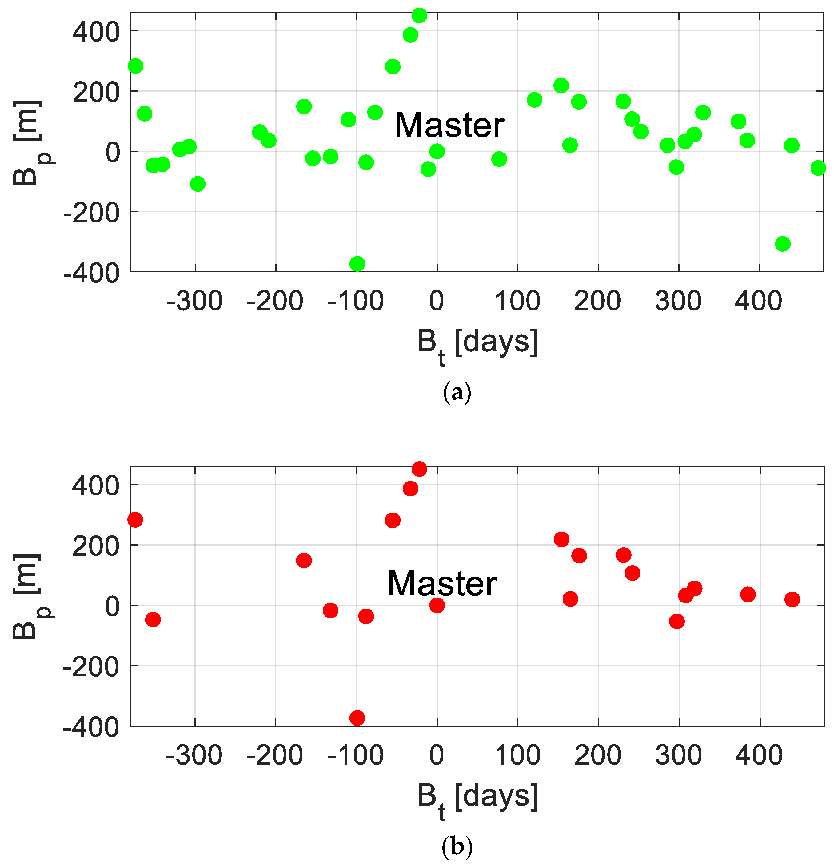
The distribution of the 39 perpendicular baselines, considered in the single polarization case vs. the temporal baselines, is reported in Figure 2a, while the distribution of the 20 perpendicular baselines, considered in the dual polarization case vs. the temporal baselines, is reported in Figure 2b. The twenty baselines have been selected in such a way to refer to comparable baseline configurations.
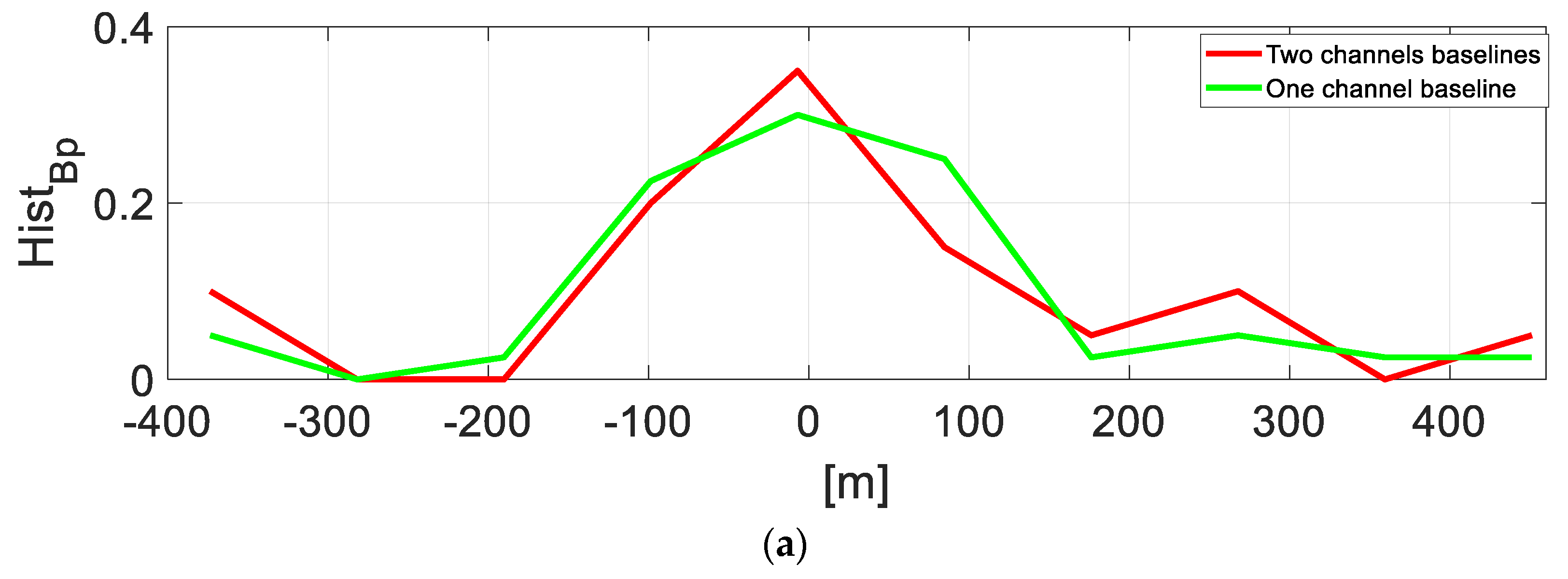
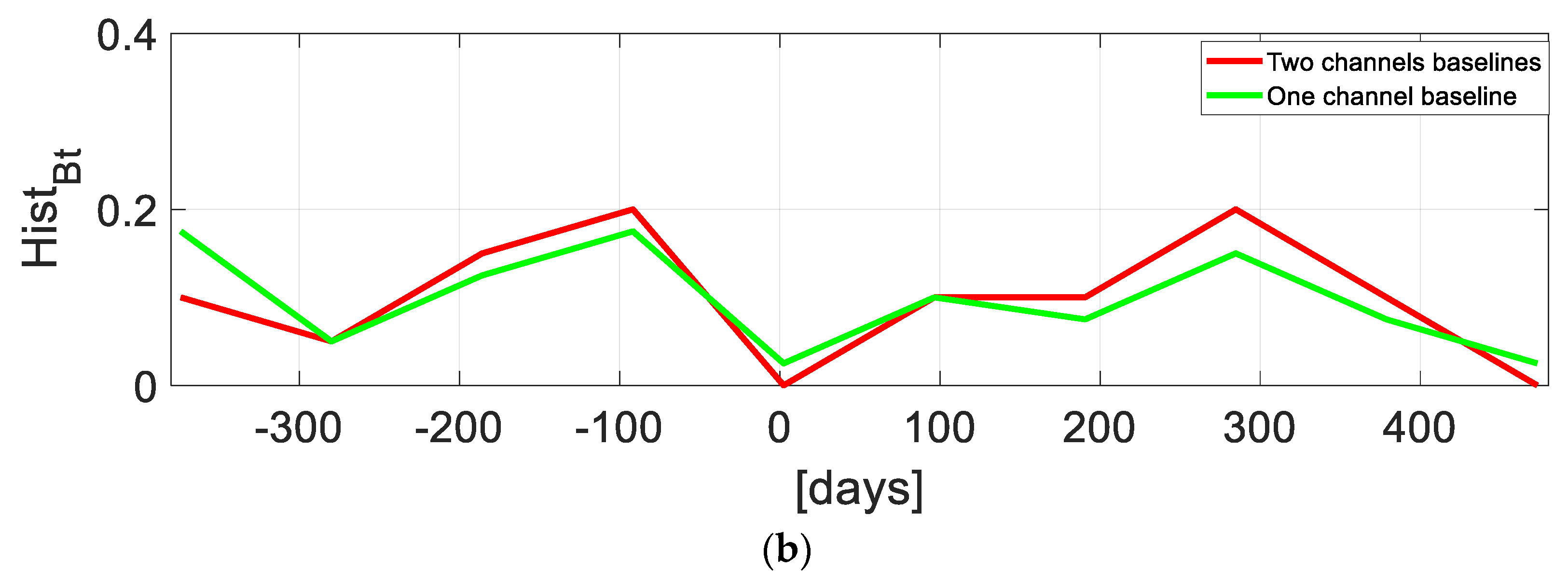
A first constraint is the maintenance of the overall perpendicular baseline span, since its value determines the achievable height resolution. This constraint is easily satisfied by selecting the two acquisitions with the minimum (negative) baseline and the maximum (positive) baseline. For the selection of other baselines, in the absence of other a priori information, we selected a subset in such a way as to have a distribution of spatial and temporal baselines similar to that considered in the 39-baseline single channel case. In Figure 3, we report the normalized histogram for the spatial (a) and temporal (b) baseline distribution (in red, the 20-baseline case and, in green, the 39-baseline case). This selection criterion should guarantee having approximately the same average spatial and temporal decorrelation in the 20- and 39-baseline datasets.
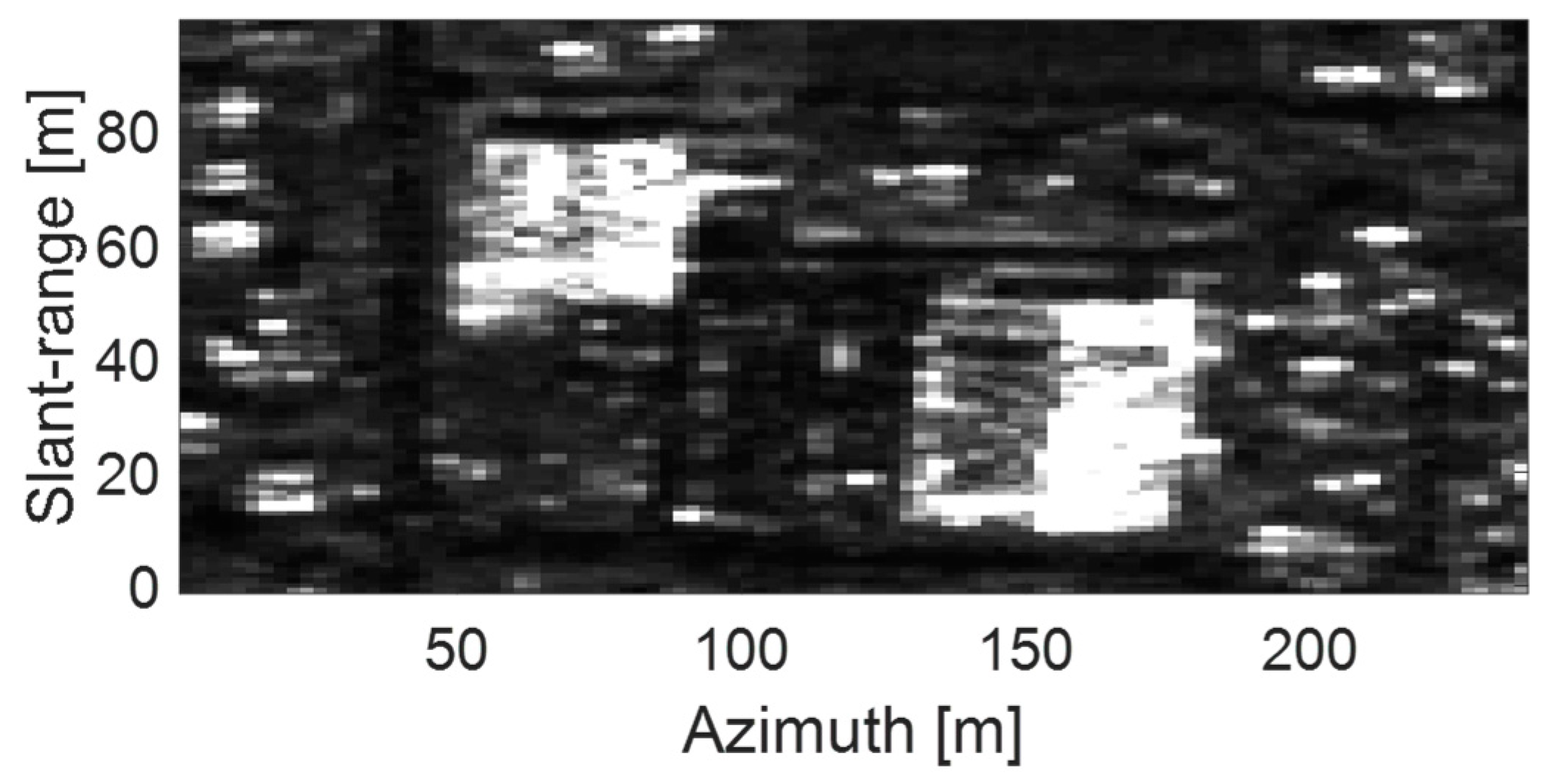
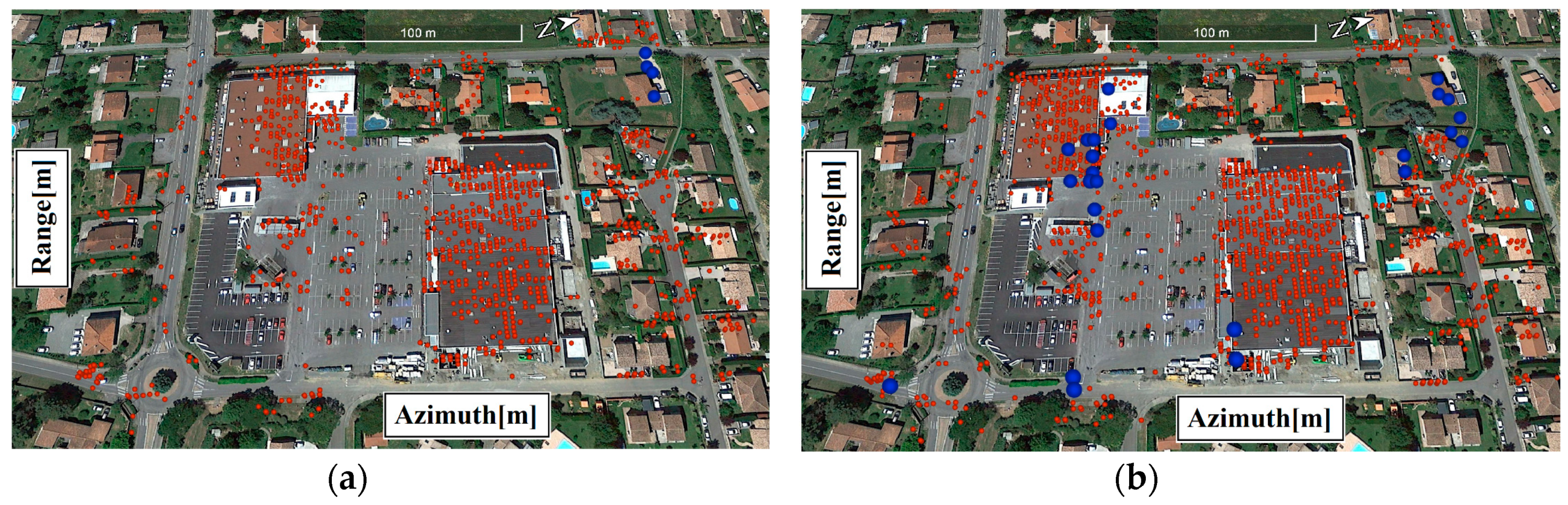
In Figure 4, the intensity HH SAR image of the test area is shown. It is a small area near Toulouse, France. Two buildings are present, and both are commercial malls, with the same height of about 10–13 m. GLRT [15] has been applied to the channel HH, considering M = 39 baselines. The thresholds have been evaluated, setting PFA = PFD = 10−4. The Rayleigh resolution in elevation is 14 m and the considered discretization step is 2 m. Since the buildings in the SAR image are not tall, we do not expect many double scatterers. There are 1328 detected single scatterers and only 2 double scatterers. The detected single and double scatterers are reported in red and blue, respectively, on the optical 3-D Google Earth image of the test area, in Figure 5a. The blue points are four, since for each double, the corresponding couple of points is reported at the estimated height in the 3-D Google Earth image. We compare these results with the case of using only 20 images but both channels HH and VV, and assuming again PFA = 10−4. In Figure 5b, the GLRT (5) has been applied considering M = 20 baselines, and the detected single scatterers are reported in red while the double scatterers are in blue, on the optical 3-D Google Earth image. There are 1733 singles, while the number of double scatterers is 13.
We observe a sensible increment of the total number of detected scatterers, which means that the diversity in polarization compensated for the diversity in baselines. In both cases, single and dual polarization, the GRLT approach is able to correctly locate the scatterers, which are mostly on the roof of the buildings; the double scatterers, where present, are coming from the interfering backscattering mechanism of ground and roof or façade and roof. In the single polarization case, very few double scatterers have been detected while, in the dual polarization case, we were able to identify, better, the double backscattering mechanism, even if we used fewer orthogonal baselines.
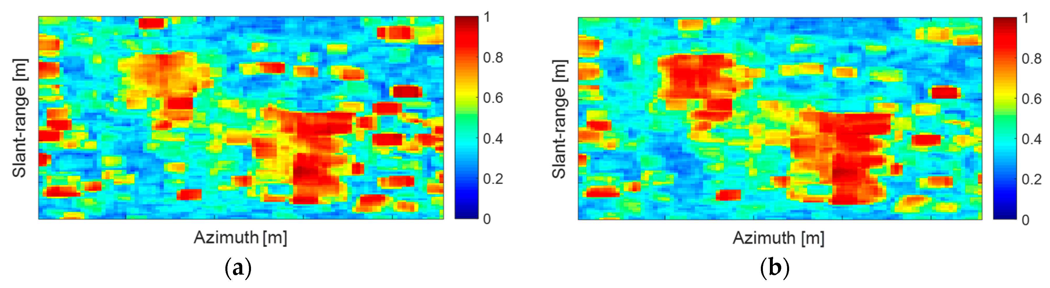
In order to find a justification as to why the single polarization approach detected less single and double scatterers, we computed the absolute values of the interferometric coherence and averaged it over all the baselines and over all the polarimetric channels. The images of these average coherence values are shown in Figure 6. We observe that, as expected, the average coherence assumes, in most of the pixels, higher values when using polarimetric data, so that a better detection performance can be achieved.
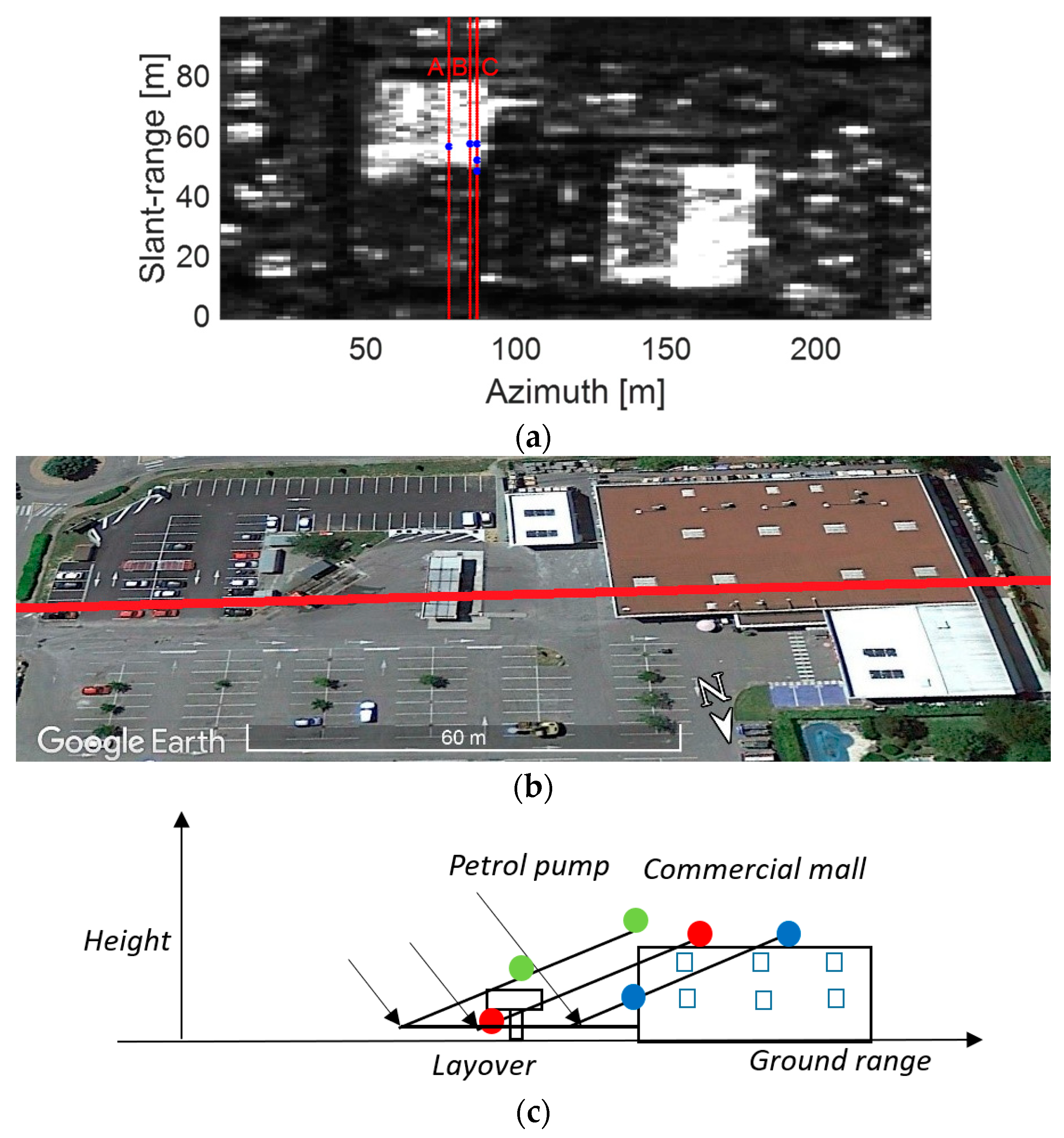
We focus now on the discussion of the results obtained in the dual polarization case. We consider three range lines corresponding to three fixed azimuth coordinates (A, B, and C, in red in Figure 7a), crossing the left side building and localized in an area where several double scatterers (in blue) were detected.
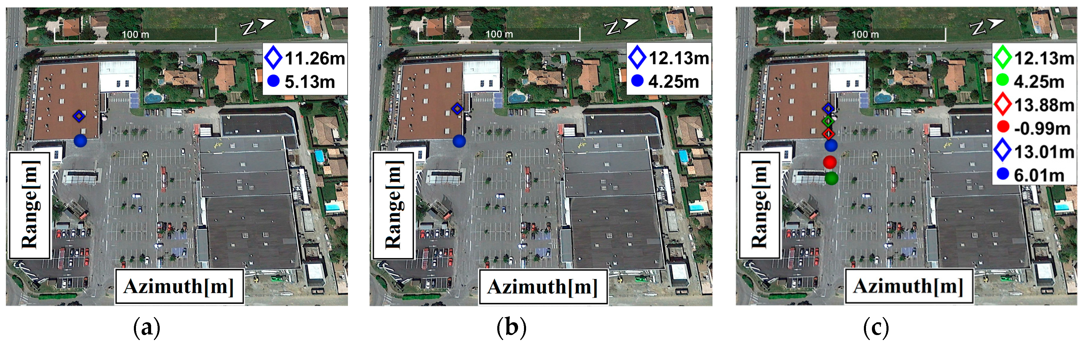
In Figure 7b,c, the scene is reported on the optical image and described by a schematic geometrical diagram, respectively. The double scatterers are reported with the corresponding heights and for the three lines, respectively A (a), B (b), C (c), in Figure 8. In the diagram in Figure 7c, we reported the double scatterers identified in the range line C with the same color used in Figure 8c. The green markers indicate the roofs of the petrol pump (estimated height is 4.25 m) and of the building ( = 12.13 m), while the ground has not been detected. The red markers indicate the ground ( = −0.99 m) and the roof of the building ( = 13.88), while the façade of the building has not been detected. Finally, the blue markers indicate the facade of the building ( = 6 m) and the roof ( = 13 m), while the ground has not been detected. We note that due to the presence of the petrol pump and the building layover effect, the true scatterers could be three in the three considered cells but, having fixed Kmax = 2, we found the two dominant scatterers.
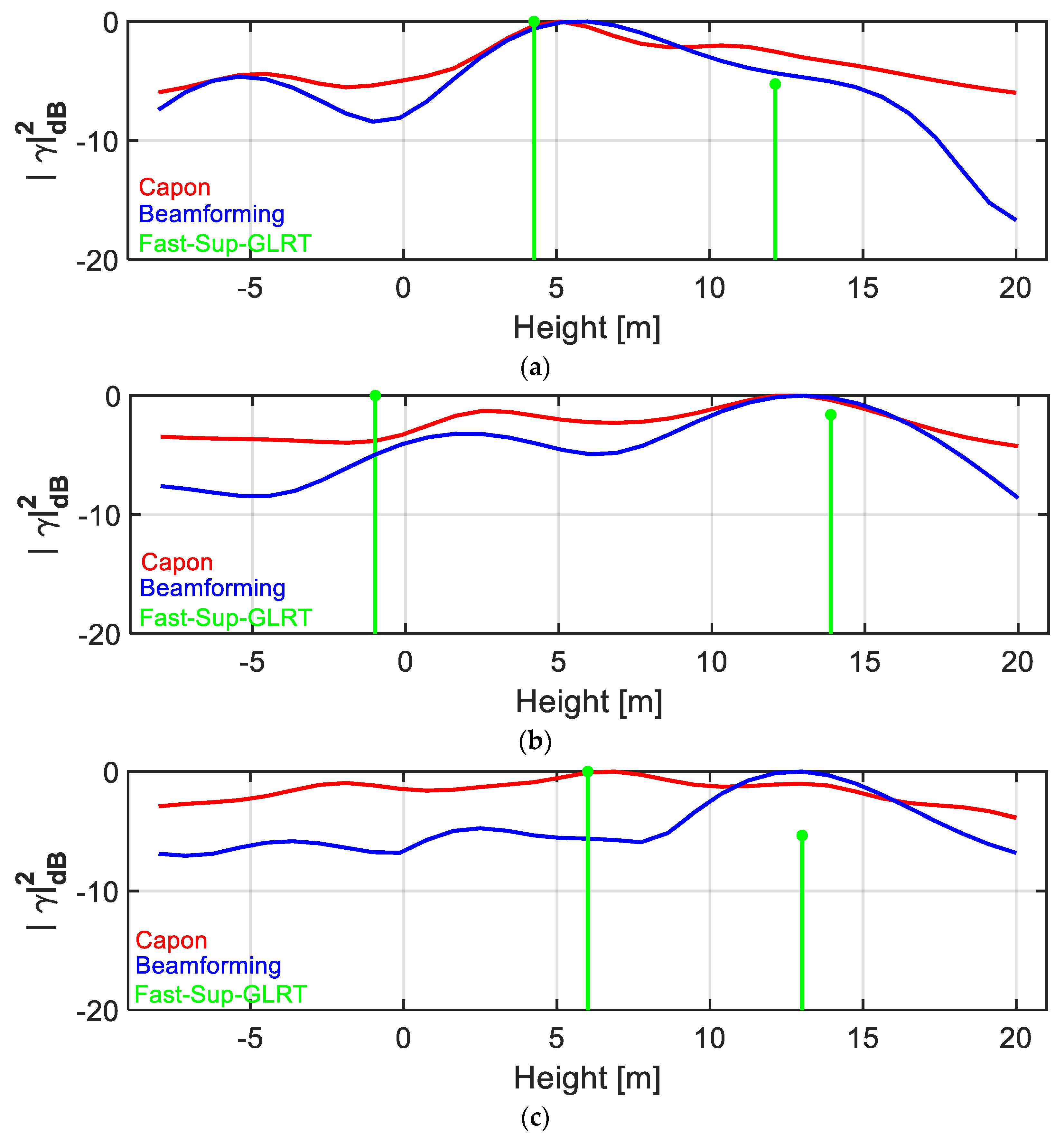
We compare now the polarimetric Fast-Sup-GLRT with the polarimetric beamforming and Capon approaches, proposed in [22]. Firstly, we consider the reflectivity profiles obtained in the three pixels of range line C where double scatterers have been detected. In Figure 9, the beamforming and Capon reconstructed spectra are reported, respectively, in blue and red. For the Fast-Sup-GLRT, we report, in green, the two estimated samples of the reflectivity profiles assumed to be 2-sparse. We note that the positions of the scatterers identified by the Fast-Sup-GLRT (in green) are very close to the first two peaks of Capon reconstruction in all three cases. In general, the beamforming lobes are broader than the Capon lobes, as expected, and the accuracy in the localization of the scatterers is worse [22].
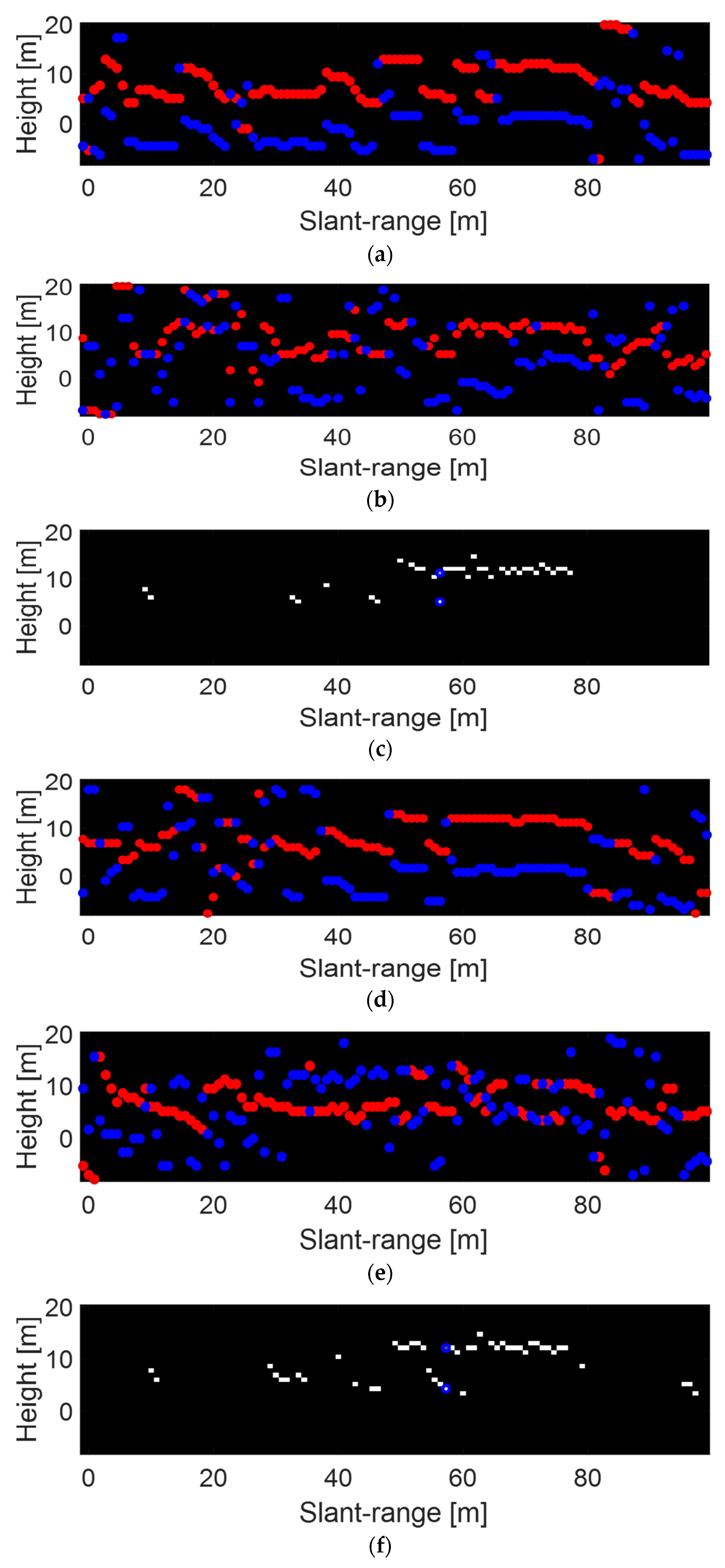
We compare also the tomographic slices obtained using polarimetric Fast-Sup-GLRT with the ones obtained applying the polarimetric beamforming and Capon approaches proposed in [22]. For the polarimetric beamforming and Capon approaches, in absence of a quality criterion, we report, in Figure 10, the values of the first two peaks (blue and red points) of the corresponding spectrum in all the points, without applying any threshold. For Fast-Sup-GLRT, we report the reflectivity values evaluated for the single and double scatterers when they have been detected. Double scatterers are shown with a blue circle. For each line, it is possible to see that, for Fast-Sup-GLRT (Figure 10c,f,i), the reconstruction is clear, since it is easy to identify the geometric profile of the building and the scattering contributions from ground and roof, and from façade and roof.
On the contrary, the tomographic reconstructions obtained with the polarimetric beamforming (Figure 10a,d,g) and with the Capon approach (Figure 10b,e,h) are difficult to interpret and appear very noisy. Around 60 m in range, the imaging of the roof of the building is quite visible in all the reconstructions. The problem is that too many peaks are visible, and the corresponding heights cannot be associated with any structure. The presence of these peaks can be explained by the use of the boxcar filter for the covariance matrix estimation, and by the sidelobe effects, due to not uniformly spaced acquisitions. In particular, double backscattering cannot be compressed in one single range pixel, but stretches over several samples, due to spatial averaging, as also reported in [22].
5. Conclusions
In this paper, we have extended Fast-Sup-GLRT tomographic processing to the polarimetric case, and validated it on spotlight TSX real data on urban areas. In particular, we have shown that the dual polarization (HH + VV) case can outperform the single polarization case (HH), keeping the number of images constant and considering, in the polarimetric case, a lower number of baselines. The dual polarization approach gains with respect to the single polarization one, since the effect of reduced baseline diversity can be compensated by polarization diversity. For each baseline, we can count on two images acquired with two different polarizations at the same time, and then, in absence of temporal changes on the ground. The proposed approach has been compared with the polarimetric beamforming and Capon approaches, showing that, without exploiting a proper selection criterion of the spectra peaks, the tomographic slices are not clearly interpretable. Focusing on a single pixel where two dominant scatterers are identified by Fast-Sup-GLRT, we have found quite good correspondence between the localizations of the two scatterers by Fast-Sup-GLRT and Capon approaches. The polarimetric beamforming method is less accurate because the spectrum exhibits broader lobes.
Author Contributions
A.B., G.S. developed the GLRT algorithm A.C.J. pre-processed real data and produced the geocoded results; all the authors contributed to performing the experiments; A.B., G.S. contributed to writing the paper.
Acknowledgments
We thank the European Space Agency (ESA), for providing software NEST. We thank for providing the TSX data the DLR (proposal MTH3182).
Conflicts of Interest
The authors declare no conflict of interest.
References
- Caltagirone, F.; Capuzi, A.; Coletta, A.; de Luca, G.F.; Scorzafava, E.; Leonardi, R.; Rivola, S.; Fagioli, S.; Angino, G.; L’Abbate, M.; et al. The COSMOSkyMed dual use earth observation program: Development, qualification, and results of the commissioning of the overall constellation. IEEE J. Sel. Top. Appl. Earth Obs. Remote Sens. 2014, 7, 2754–2762. [Google Scholar] [CrossRef]
- Porfilio, M.; Serva, S.; Fiorentino, C.; Calabrese, D. The acquisition modes of COSMO-Skymed di Seconda Generazione: A new combined approach based on SAR and platform agility. In Proceedings of the 2016 IEEE International Geoscience and Remote Sensing Symposium (IGARSS), Beijing, China, 10–15 July 2016; pp. 2082–2085. [Google Scholar]
- Lee, J.-S.; Pottier, E. Polarimetric Radar Imaging: From Basics to Applications; CRC Press: Boca Raton, FL, USA, 2009. [Google Scholar]
- Li, H.; Li, Q.; Wu, G.; Chen, J.; Liang, S. The impacts of building orientation on polarimetric orientation angle estimation and model-based decomposition for multilook polarimetric SAR data in Urban areas. IEEE Trans. Geosci. Remote Sens. 2016, 54, 5520–5532. [Google Scholar] [CrossRef]
- Hong, S.H.; Wdowinski, S. Double-bounce component in cross-polarimetric SAR from a new scattering target decomposition. IEEE Trans. Geosci. Remote Sens. 2014, 52, 3039–3051. [Google Scholar] [CrossRef]
- Gini, F.; Lombardini, F.; Montanari, M. Layover solution in multibaseline SAR interferometry. IEEE Trans. Aerosp. Electron. Syst. 2002, 38, 1344–1356. [Google Scholar] [CrossRef]
- Reigber, A.; Moreira, A. First Demonstration of Airborne SAR Tomography Using Multibaseline L-band Data. IEEE Trans. Geosci. Remote Sens. 2000, 38, 2142–2152. [Google Scholar] [CrossRef]
- Fornaro, G.; Lombardini, F.; Pauciullo, A.; Reale, D.; Viviani, F. Tomographic processing of interferometric SAR data: Developments, applications, and future research perspectives. IEEE Signal Process. Mag. 2014, 31, 41–50. [Google Scholar] [CrossRef]
- Budillon, A.; Ferraioli, G.; Schirinzi, G. Localization Performance of Multiple Scatterers in Compressive Sampling SAR Tomography: Results on COSMO-SkyMed Data. IEEE J. Sel. Top. Appl. Earth Obs. Remote Sens. 2014, 7, 2902–2910. [Google Scholar] [CrossRef]
- Zhu, X.X.; Bamler, R. Superresolving SAR Tomography for Multidimensional Imaging of Urban Areas: Compressive sensing-based TomoSAR inversion. IEEE Signal Process. Mag. 2014, 31, 51–58. [Google Scholar] [CrossRef]
- Liang, L.; Li, X.; Ferro-Famil, L.; Guo, H.; Zhang, L.; Wu, W. Urban Area Tomography Using a Sparse Representation Based Two-Dimensional Spectral Analysis Technique. Remote Sens. 2018, 10, 109. [Google Scholar] [CrossRef]
- Candes, E.J.; Romberg, J.; Tao, T. Stable signal recovery from incomplete and inaccurate measurements. Commun. Pure Appl. Math. 2006, 59, 1207–1223. [Google Scholar] [CrossRef] [Green Version]
- Pauciullo, A.; Reale, D.; De Maio, A.; Fornaro, G. Detection of Double Scatterers in SAR Tomography. IEEE Trans. Geosci. Remote Sens. 2012, 50, 3567–3586. [Google Scholar] [CrossRef]
- Budillon, A.; Schirinzi, G. GLRT Based on Support Estimation for Multiple Scatterers Detection in SAR Tomography. IEEE J. Sel. Top. Appl. Earth Obs. Remote Sens. 2016, 9, 1086–1094. [Google Scholar] [CrossRef]
- Budillon, A.; Johnsy, A.C.; Schirinzi, G. A Fast Support Detector for Super-Resolution Localization of Multiple Scatterers in SAR Tomography. IEEE J. Sel. Top. Appl. Earth Obs. Remote Sens. 2017, 10, 2768–2779. [Google Scholar] [CrossRef]
- Budillon, A.; Johnsy, A.; Schirinzi, G. Extension of a fast GLRT algorithm to 5D SAR tomography of Urban areas. Remote Sens. 2017, 9, 844. [Google Scholar] [CrossRef]
- Siddique, M.A.; Wegmüller, U.; Hajnsek, I.; Frey, O. SAR Tomography as an Add-On to PSI: Detection of Coherent Scatterers in the Presence of Phase Instabilities. Remote Sens. 2018, 10, 1014. [Google Scholar] [CrossRef]
- Tebaldini, S. Single and multipolarimetric SAR tomography of forested areas: A parametric approach. IEEE Trans. Geosci. Remote Sens. 2010, 48, 2375–2387. [Google Scholar] [CrossRef]
- Frey, O.; Meier, E. Analyzing tomographic SAR data of a forest with respect to frequency, polarization, and focusing technique. IEEE Trans. Geosci. Remote Sens. 2011, 49, 3648–3659. [Google Scholar] [CrossRef]
- Tebaldini, S.; Rocca, F. Multibaseline polarimetric SAR tomography of a boreal forest at P- and L-bands. IEEE Trans. Geosci. Remote Sens. 2012, 50, 232–246. [Google Scholar] [CrossRef]
- Pardini, M.; Papathanassiou, K. On the estimation of ground and volume polarimetric covariances in forest scenarios with SAR tomography. IEEE Geosci. Remote Sens. Lett. 2017, 14, 1860–1864. [Google Scholar] [CrossRef]
- Sauer, S.; Ferro-Famil, L.; Reigber, A.; Pottier, E. Three Dimensional Imaging and Scattering Mechanism Estimation over Urban Scenes Using Dual-Baseline Polarimetric InSAR Observations at L-Band. IEEE Trans. Geosci. Remote Sens. 2011, 49, 4616–4629. [Google Scholar] [CrossRef]
- Aguilera, E.; Nannini, M.; Reigber, A. Multisignal Compressed Sensing for Polarimetric SAR Tomography. Geosci. Remote Sens. Lett. 2012, 9, 871–875. [Google Scholar] [CrossRef]
- Budillon, A.; Schirinzi, G. Performance Evaluation of a GLRT Moving Target Detector for TerraSAR-X along-track interferometric data. IEEE Trans. Geosci. Remote Sens. 2015, 53, 3350–3360. [Google Scholar] [CrossRef]
Figure 1.
Multi-pass SAR geometry in the range–elevation plane (case M = 5).

Figure 2.
Distribution of the perpendicular baselines vs. the temporal baselines, in (a) the 39 baselines of the single polarization case, in (b) the 20 baselines of the dual polarization case.
Figure 2.
Distribution of the perpendicular baselines vs. the temporal baselines, in (a) the 39 baselines of the single polarization case, in (b) the 20 baselines of the dual polarization case.

Figure 3.
Normalized histogram of the perpendicular baseline distribution (a) and of the temporal baseline distribution (b); in green, the single polarization case and, in red, the dual polarization case.
Figure 3.
Normalized histogram of the perpendicular baseline distribution (a) and of the temporal baseline distribution (b); in green, the single polarization case and, in red, the dual polarization case.


Figure 4.
Intensity HH image of the test area near Toulouse, France (copyright DLR 2013–2015).

Figure 5.
Targets detected by Fast-Sup-GLRT and reported on the optical image (single scatterers in red, double scatterers in blue), (a) single polarization, (b) dual polarization.
Figure 5.
Targets detected by Fast-Sup-GLRT and reported on the optical image (single scatterers in red, double scatterers in blue), (a) single polarization, (b) dual polarization.

Figure 6.
Average coherence (a) single polarization, (b) dual polarization.

Figure 7.
(a) Intensity HH image of the test area near Toulouse, with three range lines highlighted in red (A, B, C), (b) range line C reported on the optical image, (c) schematic geometrical diagram of the scene.
Figure 7.
(a) Intensity HH image of the test area near Toulouse, with three range lines highlighted in red (A, B, C), (b) range line C reported on the optical image, (c) schematic geometrical diagram of the scene.

Figure 8.
The double scatterers detected by Fast-Sup-GLRT in the dual polarization case, and their estimated heights, along the three range lines A (a), B (b), C (c).
Figure 8.
The double scatterers detected by Fast-Sup-GLRT in the dual polarization case, and their estimated heights, along the three range lines A (a), B (b), C (c).

Figure 9.
Reflectivity profile obtained with beamforming (blue), Capon (red), Fast-Sup-GLRT (green), in correspondence of the three double scatterers in line C, respectively in (a–c).
Figure 9.
Reflectivity profile obtained with beamforming (blue), Capon (red), Fast-Sup-GLRT (green), in correspondence of the three double scatterers in line C, respectively in (a–c).

Figure 10.
Tomographic slices obtained with polarimetric beamforming (a,d,g), Capon (b,e,h) and Fast-Sup-GLRT (c,f,i) respectively, from top to down, for line A, B, and C. Blue circles indicate the double scatterers for the Fast-Sup-GLRT, and red and blue points respectively indicate the first and second peaks of the beamforming and Capon spectra.


Table 1.
TSX system parameters.
| System Parameters | |
|---|---|
| Wavelength | 0.031 m |
| View angle | 28° |
| Range distance | 579 Km |
| Chirp bandwidth | 120 MHz |
| Relative orbit | 48 |
| Orbit direction | descending |
| Look direction | right |
| Polarization | HH, VV |
| Perpendicular baselines extent | 800 m |
| Rayleigh resolution in elevation | 14 m |
© 2019 by the authors. Licensee MDPI, Basel, Switzerland. This article is an open access article distributed under the terms and conditions of the Creative Commons Attribution (CC BY) license (http://creativecommons.org/licenses/by/4.0/).
Share and Cite
MDPI and ACS Style
Budillon, A.; Johnsy, A.C.; Schirinzi, G. Urban Tomographic Imaging Using Polarimetric SAR Data. Remote Sens. 2019, 11, 132. https://doi.org/10.3390/rs11020132
AMA Style
Budillon A, Johnsy AC, Schirinzi G. Urban Tomographic Imaging Using Polarimetric SAR Data. Remote Sensing. 2019; 11(2):132. https://doi.org/10.3390/rs11020132
Chicago/Turabian StyleBudillon, Alessandra, Angel Caroline Johnsy, and Gilda Schirinzi. 2019. "Urban Tomographic Imaging Using Polarimetric SAR Data" Remote Sensing 11, no. 2: 132. https://doi.org/10.3390/rs11020132
Note that from the first issue of 2016, this journal uses article numbers instead of page numbers. See further details here.