A Patch-Based Light Convolutional Neural Network for Land-Cover Mapping Using Landsat-8 Images


Department of Civil and Environmental Engineering, Seoul National University, 1 Gwanak-ro, Gwanak-gu, Seoul 08826, Korea
*
Author to whom correspondence should be addressed.
Remote Sens. 2019, 11(2), 114; https://doi.org/10.3390/rs11020114
Submission received: 7 December 2018
/
Revised: 4 January 2019
/
Accepted: 4 January 2019
/
Published: 9 January 2019
(This article belongs to the Special Issue Advances in Representation Learning for Remote Sensing Analytics (RLRSA))
Abstract
:This study proposes a light convolutional neural network (LCNN) well-fitted for medium-resolution (30-m) land-cover classification. The LCNN attains high accuracy without overfitting, even with a small number of training samples, and has lower computational costs due to its much lighter design compared to typical convolutional neural networks for high-resolution or hyperspectral image classification tasks. The performance of the LCNN was compared to that of a deep convolutional neural network, support vector machine (SVM), k-nearest neighbors (KNN), and random forest (RF). SVM, KNN, and RF were tested with both patch-based and pixel-based systems. Three 30 km × 30 km test sites of the Level II National Land Cover Database were used for reference maps to embrace a wide range of land-cover types, and a single-date Landsat-8 image was used for each test site. To evaluate the performance of the LCNN according to the sample sizes, we varied the sample size to include 20, 40, 80, 160, and 320 samples per class. The proposed LCNN achieved the highest accuracy in 13 out of 15 cases (i.e., at three test sites with five different sample sizes), and the LCNN with a patch size of three produced the highest overall accuracy of 61.94% from 10 repetitions, followed by SVM (61.51%) and RF (61.15%) with a patch size of three. Also, the statistical significance of the differences between LCNN and the other classifiers was reported. Moreover, by introducing the heterogeneity value (from 0 to 8) representing the complexity of the map, we demonstrated the advantage of patch-based LCNN over pixel-based classifiers, particularly at moderately heterogeneous pixels (from 1 to 4), with respect to accuracy (LCNN is 5.5% and 6.3% more accurate for a training sample size of 20 and 320 samples per class, respectively). Finally, the computation times of the classifiers were calculated, and the LCNN was confirmed to have an advantage in large-area mapping.

1. Introduction
Land-cover mapping is one of the most essential applications of remote sensing, and its importance has been affirmed by a growing number of social and natural scientists who are utilizing land-cover maps to acquire critical information about issues such as urban planning [1,2], carbon-cycle monitoring [3,4], forest monitoring [5,6,7], and various multidisciplinary studies [8,9,10]. The value of the knowledge obtained from such studies relies heavily on the credibility of the underlying land-cover maps [11,12]. However, land-cover classification entails misclassification, and these errors propagate in downstream studies [11,13]. While these errors are actually large and mislead subsequent studies, they cannot be easily corrected once the land-cover map has been produced [14,15,16,17,18]. Thus, enormous efforts to improve the accuracy of land-cover classification have been ongoing in the remote-sensing community [19,20,21].
Land-cover classification, in general, consists of several consecutive procedures, from the acquisition of data and sampling design to classifier selection and performance evaluation [19]. Although each procedure should be well-established and affects the classification results, the major procedure of concern is the selection of the appropriate land-cover classification algorithm [21]. Naturally, numerous studies over several decades have been conducted to identify which classification algorithm is the best for land-cover mapping [21,22,23,24,25,26,27]. However, the various studies that have undertaken this issue have not been consistent in determining the best classification algorithms [21]. This is because the image types and test sites differ from study to study, and the results vary depending on whether the ancillary data is used and site-specific factors that determine the land-cover classes and legend criteria [19,21,28]. In addition, comparisons that lack a sufficiently thorough search for the optimal classifier parameter can mislead the results [23,29]. Moreover, since the sensitivity of an algorithm to the training sample size varies, the superiority of the classifiers is not easily determined [22,24]. Because these confounding factors impede an integrated conclusion, the remote-sensing community has been suffering from the inability to select the most suitable classifier.
Some studies have provided a general description of classifiers, along with their strengths and weaknesses, to reduce the confusion associated with classifier selection. Lu and Weng [19] gave a detailed description of the general procedure and major classifiers for land-cover mapping, and they explained the factors influencing classification performance. Li et al. [24] observed the importance of parameter setting and training sample sizes by comparing 15 classifiers in the same Landsat thematic mapper (TM) image acquired over Guangzhou City, China. Additionally, Maxwell et al. [27] provided a general description of several machine-learning algorithms for land-cover classification. A hyperspectral image and a high-resolution aerial image were used to explain the requirements of each classifier, parameter selection, and computational cost. These previous studies have assisted the classifier selection process by describing the features of the classifiers and the important factors to be considered for successful classification, such as parameter optimization and training sample sizes; however, since quantitative comparison was not the aim of these studies, it is still difficult to compare their performance.
In order to quantitatively compare the performance of different classifiers, a meta-analysis was performed by controlling the confounding factors. Khatami et al. [21] provided a quantitative ranking of the relative accuracy of the classifiers. Through the last 15 years of meta-analysis on supervised per-pixel classifications published in five high-impact remote-sensing journals, it was observed that the support vector machine (SVM) achieved the greatest accuracy, followed by neural networks (NNs) and k-nearest neighbors (KNN). The results serve as a good guideline for explaining the general superiority rankings among classifiers, but the hierarchy of the classifiers derived from the Khatami et al. [21] study represents the combined results of studies at various resolutions, some of which use ancillary data. On the other hand, most land-cover maps have been produced from medium-resolution images with a pixel size of 30-m without the use of ancillary data [20]. This is because Earth observation images with 30-m resolution have been extensively accumulated for several decades [6,30,31,32], and it is difficult to use ancillary data appropriately because of registration issues [28]. Therefore, it is imperative to confirm the superiority of the classifiers in medium-resolution land-cover mapping with only spectral inputs.
Another notable point is that the performance of classifiers differs depending on whether pixels or objects are used as classifying units for land cover mapping [33,34]. Recent studies comparing pixel-based and object-based classification at high-resolution images reveal that the latter outperforms the former in general [33,35,36]. However, classification accuracies between pixel-based and object-based classification were not statistically significant in 10-m resolution SPOT-5 image [34]. Also, pixel-based SVM was more accurate than object-based classifier in 30-m resolution Landsat images [37]. This is because the distinct advantages of object-based classification cannot be employed with medium-resolution (larger than 10-m) images due to the coarse resolution [38,39]. Therefore, this study excluded object-based classification and was limited to supervised classification in medium-resolution (30-m) images.
There have been studies comparing the performance of classifiers in medium-resolution images. He et al. [26] used Landsat images and compared the performance of the SVM, NN, random forest (RF), and maximum likelihood classifier (MLC). These classifiers were used to classify Landsat images of the lithological area, including 13 land-cover classes. This study reported that SVM produced the highest average overall accuracy, followed in order by NN, RF, and MLC. Thanh Noi and Kappas [22] compared the performance of SVM, KNN, and RF with a single Sentinel-2 image without using ancillary data. The test site was a peri-urban area of 30 km × 30 km consisting of six land-cover types, and the comparison was conducted with 14 different training sample sizes. Their study found that SVM produced the highest overall accuracy in 13 out of 14 training samples when an exhaustive search for the proper parameter was made. Although these two studies were limited to specific regions, the classification accuracy was compared with thoroughly tested procedures, and SVM outperformed the other classifiers.
To overcome the limitations of regionally specific results, some studies have compared the best-performing classifiers under various landscapes. Gong et al. [40] conducted a land-cover classification on over 8900 scenes of Landsat images covering most of the world’s land surface to compare the performance of an SVM, decision tree classifier (J4.8), RF, and MLC. They reported that the SVM produced the highest overall accuracy, followed by RF, J4.8, and MLC. Recently, Heydari and Mountrakis [25] analyzed classifiers’ performances on 26 test blocks of Landsat TM images with an area of 10 km × 10 km for each test block. An SVM, KNN, bootstrap-aggregation ensemble of decision trees (BagTE), and NNs with optimized parameters were compared. They observed that the SVM with optimized parameters was the best classifier in 18 out of 26 cases and recommended using SVM or KNN for classifications when using Landsat’s spectral inputs because of the computation time. In the previous studies up to this point, an SVM with proper parameters has generally obtained the highest accuracy of all the classifiers. Meanwhile, NNs have not performed better than SVM has, in terms of accuracy and computation time, when using only multispectral inputs [25,26,41,42]. This is because NNs did not exhibit any distinct advantage with a low number of features when confined to multispectral inputs, and they did not overcome the overfitting problem, which indicates that the network becomes so overly specific to its complexity due to imperfect training samples that it results in an inability to generalize well to unseen data [43,44,45].
Recently, a convolutional neural network (CNN), a special type of NN, has achieved overwhelming performance improvements over previous algorithms and has made breakthroughs in the field of image classification [46]. By using the concept of local connectivity and parameter sharing through layers, it has successfully overcome the overfitting problem, which is the major problem of NNs [47]. Studies on the performance of CNNs have also been conducted with remote-sensing images and have attained promising results [48,49], but most of the research has exceedingly focused on high-resolution images and hyperspectral images [50,51,52]. This bias is because the salient advantage of CNNs is their ability to efficiently handle a large amount of complicated data by preventing the overfitting problem [47,48,49].
The first study to use a CNN for medium-resolution land-cover classification was conducted by Sharma et al. [53], who proposed a patch-wise performing deep CNN (DCNN) that extracts image patches and classifies the center pixel of each patch. Landsat-8’s spectral inputs and the Florida Everglades area, which consists of eight land-cover classes, were used for the performance evaluation. The DCNN obtained higher accuracy than the pixel-based SVM did. However, because of its deep complex structure, this network required too many training samples in order to avoid overfitting and necessitated heavy computation. Moreover, Sharma et al. [46] compared patch-based DCNN against pixel-based classifiers. Although both patch-based and pixel-based systems predict the label of one pixel, they do not use the same input for training and testing. Thus, direct comparison of patch-based DCNNs and pixel-based classifiers is not valid because it does not lie on the same baseline. Therefore, it is necessary to verify the performance of patch-based CNNs with a tenable comparison to other classifiers, including patch-based systems, and propose a well-fitted CNN for medium-resolution land-cover mapping that achieves high accuracy with a practical number of training samples.
In this paper, a light convolutional neural network (LCNN) for medium-resolution land-cover mapping, attaining high accuracy with the spectral input of Landsat-8 images, is proposed. The LCNN can achieve high accuracy without overfitting, even with a small number of training samples. It has low computational cost because of its much simpler design compared to conventional CNNs that are used for high-resolution or hyperspectral image classification tasks. Both patch-based and pixel-based systems of SVM, KNN, and RF with optimized parameters were compared to the LCNN for an impartial comparison. Also, the DCNN for a medium-resolution land-cover classification proposed by Sharma et al. [53] was compared with our proposed LCNN. Three test sites of Landsat-8 images with 30 km × 30 km dimensions, including a wide range of land-cover types and five different training sample sizes (20, 40, 80, 160, and 320 samples per class), were utilized to confirm the generalization capability of the LCNN and the effect of the training sample sizes. Moreover, by introducing a heterogeneity value measuring the map’s complexity, we demonstrated the comparative advantage of LCNNs over pixel-based classifiers. Lastly, the computation times of the classifiers were reported, and the LCNN was found to be advantageous, especially in mapping large areas.
2. Datasets and Methodology
2.1. Datasets
We used the National Land Cover Database (NLCD), a product of the Multi-Resolution Land Characteristics Consortium (http://www.mrlc.gov), for reference data. The NLCD is a well-established and widely used source for land-cover classification studies [6,42,54,55]. The most recent NLCD product release, NLCD 2011, includes 16 land-cover classes (https://www.mrlc.gov/data/nlcd-2011-land-cover-conus). Wickham et al. [16] recently estimated the overall accuracies of NLCD products and showed that the overall accuracy of the NLCD 2011 individual date products was 88% at the 8-class (Level I) and 82% at the 16-class (Level II) hierarchical levels [56]. We used Level II products from NLCD 2011, which is a subdivision of the Level I NLCD, as reference data. In order to evaluate the performance of classifiers while avoiding site-specific results, we selected three 30 km × 30 km test sites covering diverse classes of the NLCD 2011 including a megacity, mountainous areas, and croplands. Each test site contained several classes consisting of less than a few thousand pixels. These pixels were excluded from the experiment so as to maintain enough samples for the experiment. The three test sites used in this experiment are shown in Figure 1. Each test site consists of 10, 8, and 8 land-cover classes, respectively, and a total of 15 land-cover classes were tested in this experiment.
One Landsat-8 image with few clouds for each test site was used for the classification. We excluded thermal bands due to their coarser resolutions, and band 9 was also excluded because it is a band meant for cirrus cloud detection [57]. The rest of the 30-m resolution bands of Landsat-8 Operational Land Imager (OLI) were included so that the classifiers could perform better using richer features [24]. Thus, we used seven bands (i.e., band 1 to 7: ultra blue, blue, green, red, near infrared, shortwave infrared 1, and shortwave infrared 2) of Landsat-8 OLI with a resolution of 30-m. These seven bands were acquired as radiance value and rescaled to the range of [0,1] by min–max normalization, which is a general procedure used in machine learning algorithms [58,59]. The min–max normalization is done using the following formula:
where is the pixel radiance of the ith band of Landsat-8 images. Atmospheric correction was not conducted because a single-date image with a clear sky was used.
2.2. Sampling Design and Comparison Scheme
Figure 2 presents the procedure from the sampling design to the comparison scheme to evaluate the performance of the LCNN. We randomly sampled five different sample sizes with 20, 40, 80, 160, and 320 samples per land-cover type for each test site, called the “sampled datasets”, in order to prepare the data for training and validation. Each sampled dataset is divided into 70% of the training set and 30% of the validation set. The training set was used to train the classifier, and the validation set was used to select the best model of each classifier for accuracy assessment. The test set was also randomly sampled with 1000 samples per each land-cover type to test the classification performance. To increase the statistical confidence of the results, random samplings for the sampled datasets and test sets were mutually exclusive and replicated 10 times to perform classification for every case (i.e., three test sites with five different sample sizes). Moreover, all the samples for training, validation, and test sets were randomly selected from the whole image of each test site including the pixels at the class borders. This is because mixed pixels also should be classified eventually and their presence does not significantly decrease the classification accuracy [60,61].
A patch-based sample differs from a pixel-based sample in shape because a sample comprising surrounding pixels is drawn. However, since only the groundtruth of the central pixel of each patch is investigated for sampling, the same number of groundtruths is required as in the pixel-based system. In order to make a valid comparison, the center of the patch is matched to the sample of the pixel-based system for every random sampling. For the patch-based system, two different patch sizes were used (sizes three and five). In sum, three different sample sizes (1 × 1 × 7 for the pixel-based system; 3 × 3 × 7 and 5 × 5 × 7 for the patch-based system) were trained and tested, and the centers of the three types of samples coincide.
As a result, a total of 13 algorithms (i.e., the two sizes of patch-based samples, 3 × 3 × 7 and 5 × 5 × 7, with LCNN, DCNN, SVM, KNN, and RF, and the pixel-based sample, 1 × 1 × 7, with SVM, KNN, and RF) performed land-cover classifications to evaluate the performance of the LCNN. To further explore the characteristics of the LCNN in detail, the performances of the algorithms were compared in three aspects: the overall accuracy, the accuracy according to the heterogeneity value, and the computation time.
2.3. Light Convolutional Neural Network
A CNN is composed of multiple layers that allow the network to learn high-level abstract features from the massive input data. Due to the distinctive advantage of the CNN extracting features from a large amount of intricate data through consecutive layers, most CNNs have a deep structure of multiple layers with a large number of filter weights [62]. However, the increase in the number of layers and filters increases the number of parameters to be learned, which also increases the computational cost and requires a large number of training samples in order for the network to perform well without overfitting [47]. Therefore, a network of appropriate complexity should be designed according to the objective and the data type to be learned.
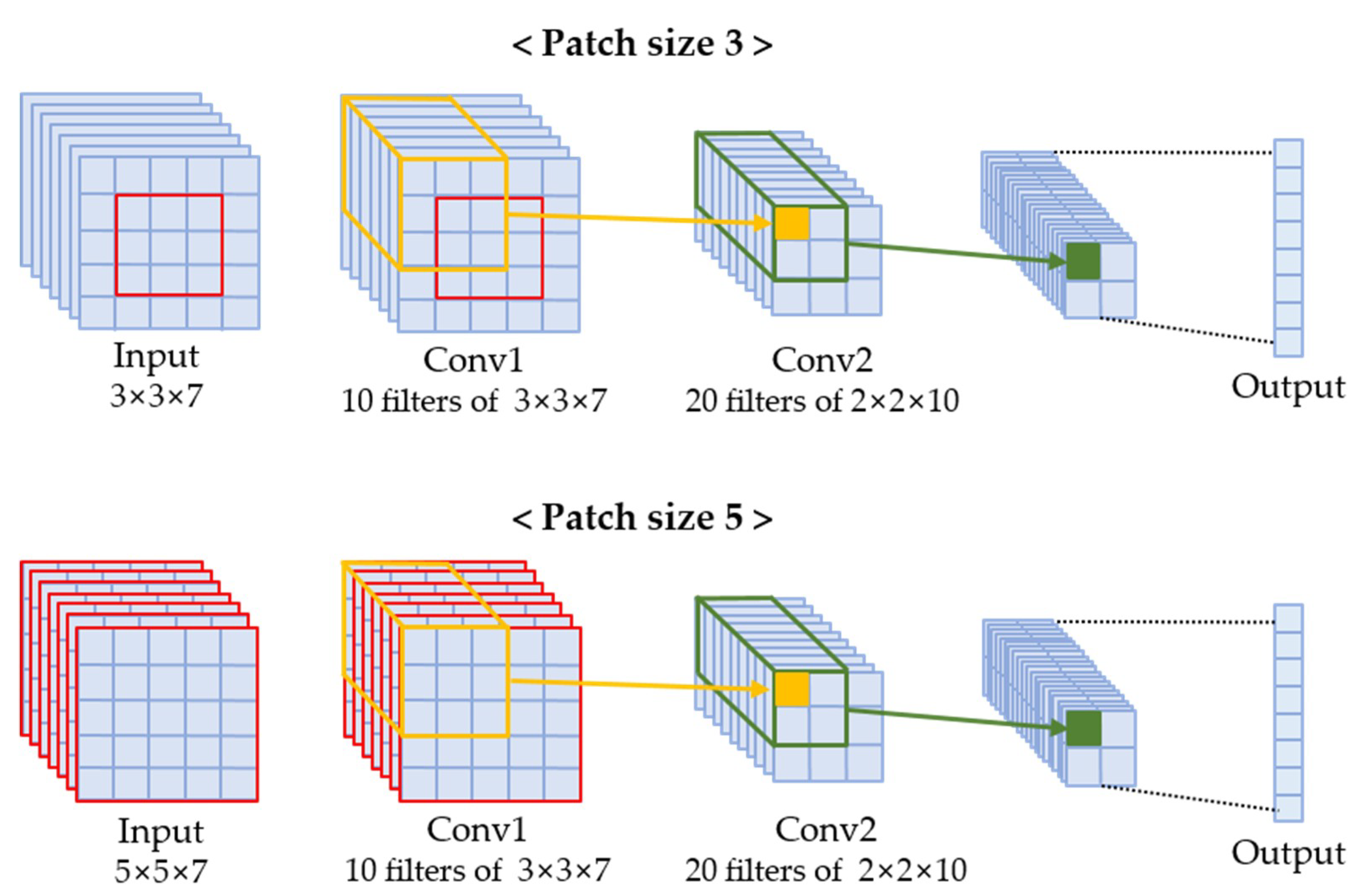
We propose the LCNN appropriate for the medium-resolution land-cover mapping task. The LCNN can learn feature representations from the patches without overfitting, even with a small number of training samples, and can achieve high accuracy due to its simple but sufficient model capacity to learn deep features from multispectral inputs. The proposed architecture is shown in Figure 3. The LCNN uses 3D samples (patch size × patch size × the number of bands) as inputs. In our test, we experimented with patch sizes of three and five, and seven Landsat-8 OLI multispectral bands were used. The first convolutional layer filters the 3D input patches with 10 filters of size 3 × 3 × 7. The filters shift horizontally and vertically with a stride of one on the 3D samples. These filters compute the dot product of their weights and the input pixels and create 10 new feature maps. In turn, the second convolutional layer takes the output of the first convolutional layer as its input. The second convolutional layer filters with a stride of one using 20 filters of size 2 × 2 × 10. Since we used a zero padding of one for the patch size of three, its operation is the same as that of a patch size of five. Thus, both patch size inputs result in 80 features from the pairs of convolutional layers. Then, the 80 features are directly fed into the softmax layer to provide a probability distribution over different land-cover classes. Inspired by the NiN [63] architecture, we omitted the fully connected layers, which increase the computational cost and the chance of overfitting. Also, a pooling layer was not used because the LCNN learns from small patch-based samples. ReLU (Rectified Linear Unit) was used for the activation function, and the Adam optimizer [64] with a learning rate of 0.001 was adopted for the optimization of the loss function.
By configuring only two convolutional layers with small numbers of filters, the number of LCNN trainable parameters could be less than 3000, which is less than one-thousandth of the number of parameters for the DCNN proposed by Sharma et al. [53] and less than a thousandth to ten-thousandth of that of several well-known benchmark networks, such as AlexNet [46], VGGNet [65], and GoogLeNet [66]. With a simple and light design, the LCNN can achieve high accuracy even with a small number of training samples without overfitting. This means that the LCNN has a suitable complexity for medium-resolution land-cover mapping tasks.
2.4. Parameter Optimization and Experimental Setup
In order to perform a fair comparative evaluation, each classifier should be optimized with parameters that can achieve the best of a classifier’s attainable accuracy. Even with the same kind of data (multispectral input), the optimal parameter varies depending on the test site and the training samples. Therefore, we tried to allow each classifier to attain their maximum accuracy for every case using grid search. We performed tests with various parameter combinations by investigating the parameters used in previous studies [22,24,25,42]. The parameter combinations used for each classifier are reported in Table 1. Among the combinations, the optimal combination for each case was found by using the validation set. In turn, the classifiers with their optimal parameters were used to obtain overall accuracy for comparison by using test sets. For DCNN, ReLU was used for the activation function, and the learning rate was set to 0.0001 with the Adam optimizer as described in the paper [53].
Implementations of SVM, KNN, and RF were supported by the scikit-learn library [67], and LCNN and DCNN were implemented based on Google’s Tensorflow framework [67]. The classifiers were carried out on Intel(R) i7-6700 3.40-GHz CPU with 32 GB RAM memory. For CNNs, one GeForce GTX 1080Ti graphics processing unit (GPU) with 11 GB memory was also used.
3. Results
3.1. Classification Accuracy in Three Test Sites for Five Training Sample Sizes
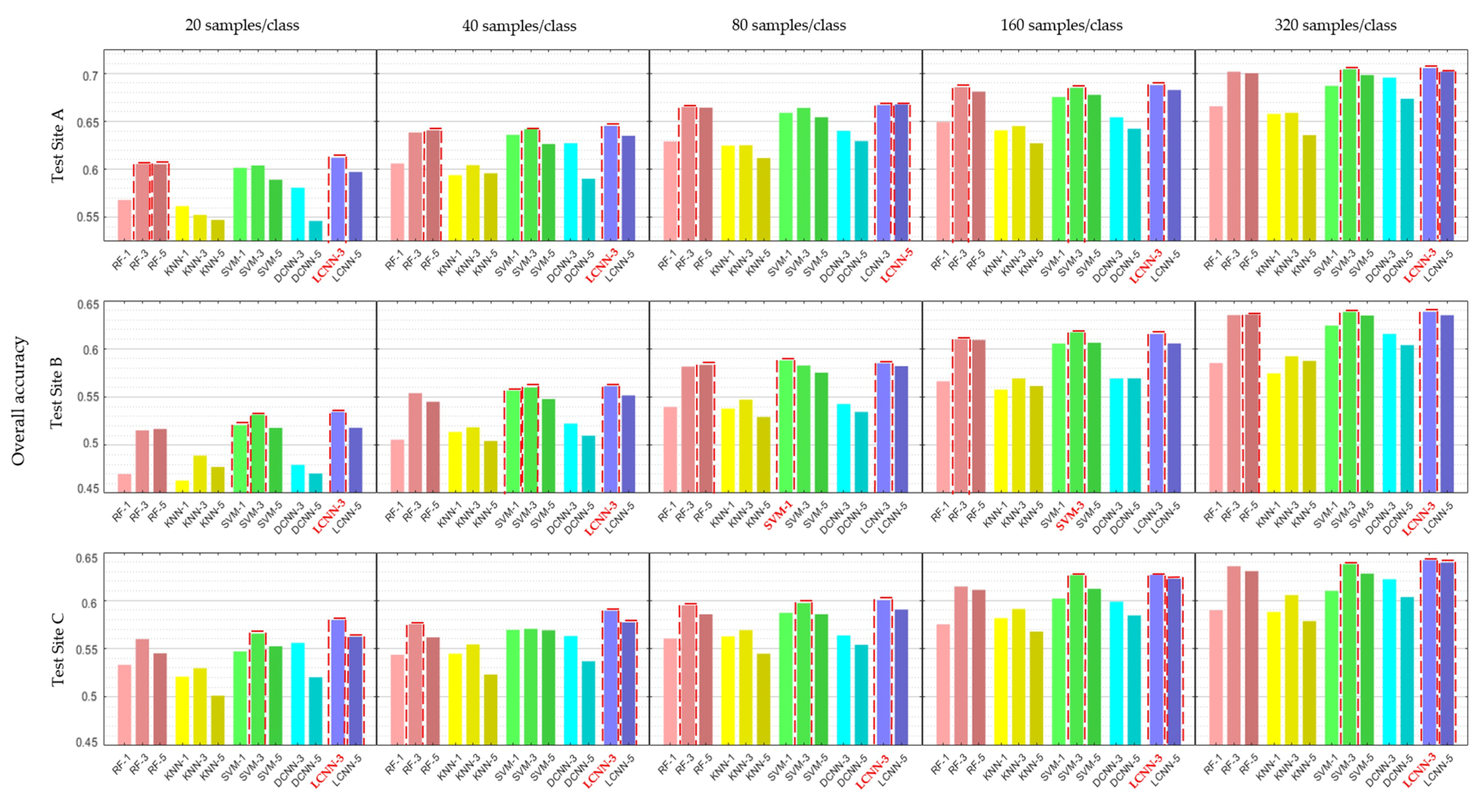
Classifiers were compared in a total of 15 cases. Figure 4 reports the average of the overall accuracy obtained from 10 repetitions of every 15 cases. The proposed LCNN with a patch size of three (referred to hereafter as LCNN-3) attained the highest accuracy in 12 out of 15 cases. In the three exceptions, an LCNN with a patch size of five, an SVM with a patch size of three, and an SVM with a pixel-based system had the highest accuracies. This result indicates that the LCNN-3 was successfully designed for land-cover mapping with sufficient model capacity to attain high accuracy without overfitting with small sample sizes due to its light design. On the other hand, the DCNN did not achieve high accuracy. This failure can be explained by overfitting due to insufficient training samples compared to its deep complex structure. The DCNN was able to obtain high accuracy only if there were hundreds of thousands of training samples, as reported in the Sharma et al. paper [53].
The average overall accuracy of each classifier according to sample size and the total average overall accuracy of each classifier in 15 cases are shown in Table 2. Since all classifiers were trained and tested with 10 different random samples for every case (i.e., three test sites with five different training samples), we could obtain a total of 150 classification results from each classifier. With 150 results from each classifier, the pairwise one-sided p-values to test significant differences between LCNN-3 and the others were calculated using paired t-tests in Table 2. Results show that the LCNN-3 attained the highest average overall accuracy in every sample size. Also, the LCNN-3 produced the highest overall accuracy of 61.94% on average for a total of 150 cases; this was followed by SVM (61.51%) and RF (61.15%) with a patch size of three. Although the accuracy difference between the classifiers becomes smaller as the number of training samples increases, the LCNN-3 consistently obtained higher accuracy than did the other classifiers. Noting the fact that the difference in accuracy obtained from the sample size of 160 per class and 320 per class is not large compared to the large increase in the number of training samples, the classifiers were given enough training samples (320 per class) to reach their best attainable accuracy. This is also supported by the findings of previous studies [24,42,55] that showed that the accuracy difference between classifiers becomes smaller as the number of training samples becomes greater than about 200 samples per class, and the accuracy then converges to some extent. Therefore, these results indicate that the LCNN-3 provided consistently superior classification accuracy over various sample sizes, and the LCNN-3 should be favored among other classifiers.
In addition, note that all patch-based classifiers, except for DCNN, obtained higher accuracy than did the pixel-based classifiers. Also, the calculated p-values show that LCNN-3 outperformed all pixel-based classifiers at the 5% significance level. These results confirm that utilizing the neighboring pixels’ information can enhance the classification accuracy. On the other hand, all classifiers with a patch size of five obtained lower accuracy than the corresponding classifiers with patch sizes of three. Although the difference in accuracy between the two cases tends to decrease as the training sample size increases, the patch size of three achieved higher accuracy than did the patch size of five. This finding suggests that the patch size of five performance may be reduced by the Hughes phenomenon due to its large number of input variables relative to the number of training samples.
3.2. Effect of Map Heterogeneity on Classifier Performance
To explore the advantage of a patch-based performing LCNN, the heterogeneity value was calculated by the following formula:
where is the pixel coordinate of the image, and is the land-cover class at . In addition, denotes the Iverson bracket indicator function, which outputs 1 if the statement in square brackets is true, and 0 otherwise.
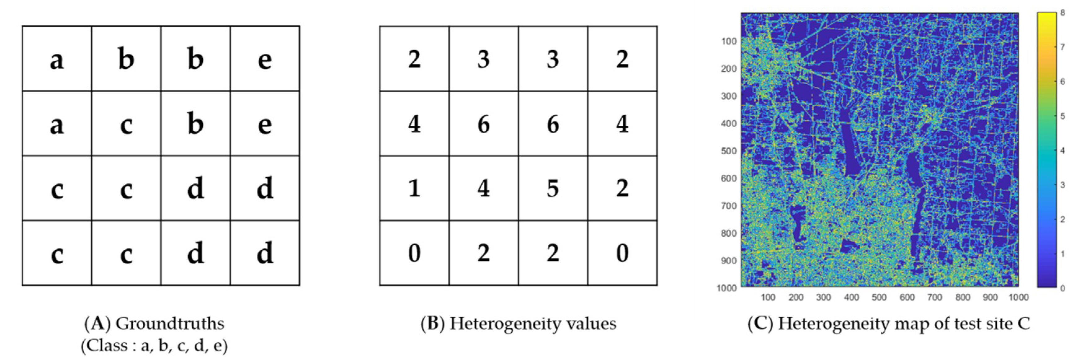
By counting the number of eight neighbor pixels with a different class from the center pixel as defined in Equation (2), the heterogeneity value describes the complexity and contextual property of the land-cover [68]. An example of calculating heterogeneity values and a case from test site C are depicted in Figure 5. By calculating the heterogeneity value in this way, all pixels have values from 0 to 8. Because the heterogeneity value (0–8) indicates the number of pixels that are different from the center pixel’s class among the eight neighbor pixels, it is reasonable to assume that the larger the heterogeneity value is, the more complex the land-cover and the more likely it is the mixed pixel. In this manner, the classification performances of algorithms were analyzed according to the heterogeneity value.
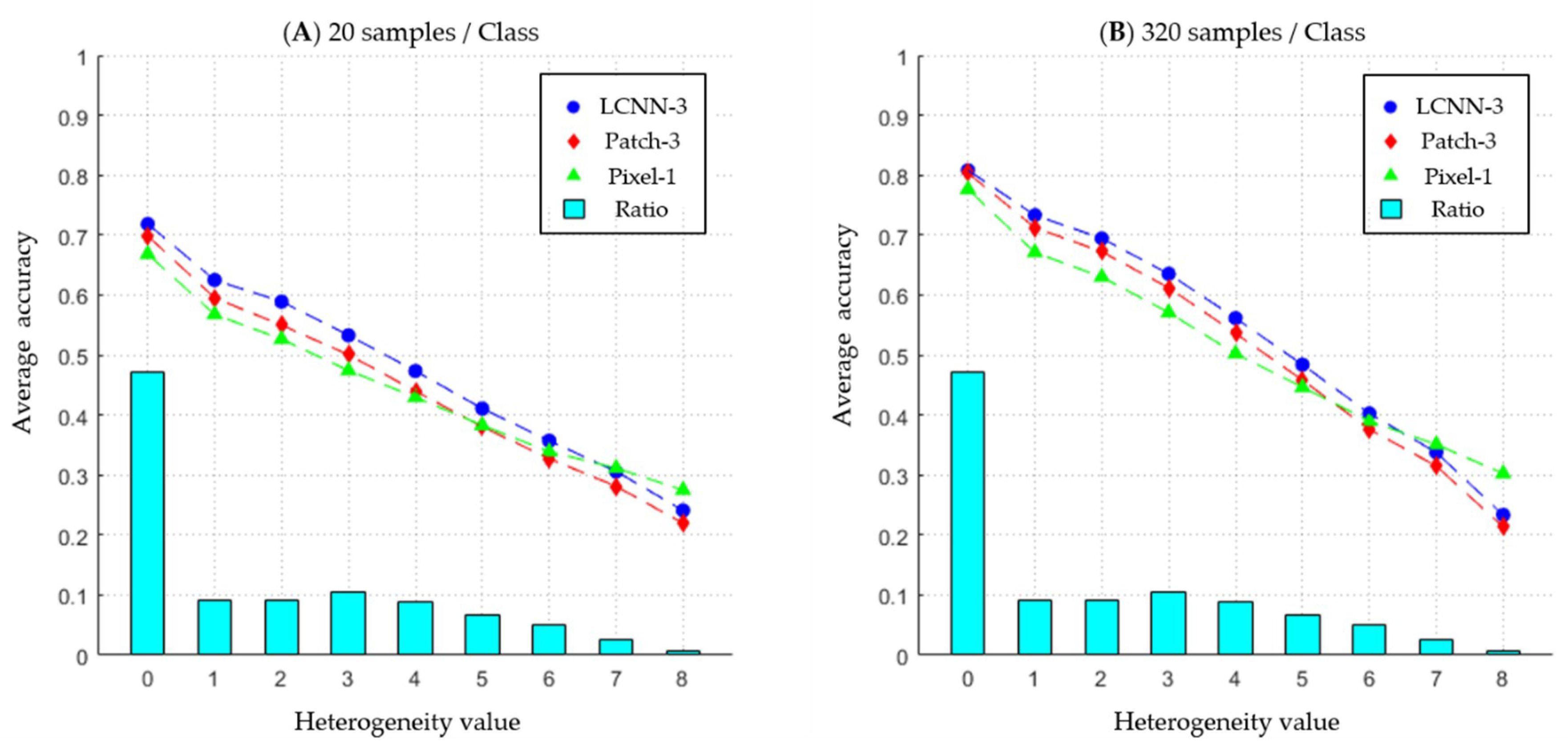
To analyze why patch-based performing LCNN is more accurate than pixel-based classifiers, and to investigate the characteristics of the LCNN more clearly, we classified the algorithms into three groups as follows: LCNN-3, Patch-3, and Pixel-1. The Patch-3 group consists of SVM, KNN, and RF with a patch size of three, and the Pixel-1 group consists of SVM, KNN, and RF with a pixel-based system. In Figure 6, the average classification accuracies of the three groups at the three test sites were calculated according to the heterogeneity values. In addition, the composition ratios of the heterogeneity values in all test sites are shown together.
Notice the accuracy discrepancies between LCNN-3 and Pixel-1 according to the heterogeneity values. When the heterogeneity value is 0, there is not much difference in accuracy (5.1% at the training sample size for 20 samples per class; 3.2% at the training sample size for 320 samples per class). However, for heterogeneity values from 1 to 4, the average accuracy discrepancy between the two is about 5.5% for a training sample size of 20 samples per class and 6.3% for a training sample size of 320 samples per class. This means that the LCNN-3 performed better than other pixel-based classifiers did, especially in moderately mixed pixels, because the LCNN-3 considered its neighbor pixels for classification.
However, when the heterogeneity value is greater than 4, the discrepancies become smaller, and they are reversed when the heterogeneity value is 7. This explains that the LCNN-3 had more difficulty in predicting severely heterogeneous pixels than pixel-based classifiers. However, the LCNN-3 obtained higher overall accuracy in total (as shown in Table 2) because the heterogeneity values of 7 and 8 make up less than 4% of all values (see the composition ratio in Figure 6). This observation indicates that the LCNN-3 outperformed the pixel-based classifiers because the LCNN-3 exploited neighbor pixels for classification. Patch-3 showed a similar tendency to LCNN-3 but obtained lower accuracy than did LCNN-3 for all heterogeneity values.
3.3. Computation Time
Computation time is divided into the time for the training phase, validation phase, and testing phase. In CNNs, there is no validation time because the parameters are fixed. A further consideration is that CNNs use a GPU when doing computations, while other classifiers do not use a GPU. Therefore, the computation time of an LCNN without using a GPU was also reported to provide fair comparison results. The average computation time of the three test sites with 10 iterations at two training sample sizes (20 and 320 samples per class) is reported in Table 3. The result of the KNN and classifiers with patch sizes of five are omitted because of their lower accuracy.
As a result, the LCNN without a GPU took less time to perform training and testing than did the LCNN with a GPU. It can be reasoned that the parallel computation is rather inefficient because the LCNN requires little computation due to its light design. In general, regardless of whether the GPU was used, the LCNN took a much longer time than the other classifiers did for the training phase, except for the DCNN. When it comes to the testing phase, however, the LCNN took less time than the other classifiers did. Note that the testing time of the LCNN does not increase as the training sample size increases. This is because the computation complexity of the CNN is fixed irrespective of the training sample sizes. Considering that the number of test samples is fixed to 1000 pixels for each class, the LCNN can perform more quickly with high accuracy than can other classifiers, especially when mapping a large area with a sufficient number of training samples.
4. Discussion
4.1. Classification Performance of LCNN According to Land-Cover Classes
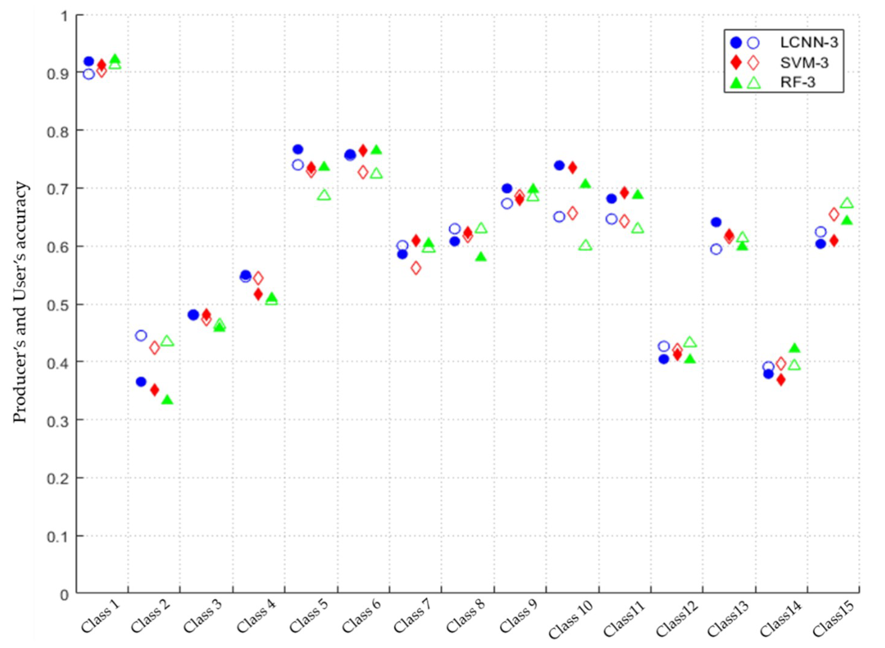
To further discover the classification performance of LCNN-3 according to land-cover classes, the producer’s and the user’s accuracy (i.e., the complementary measures of the omission and commission errors, respectively) of each class were investigated. By integrating and averaging the results from the three test sites with five different sample sizes and 10 iterations for each, the producer’s and the user’s accuracies for 15 land-cover classes could be calculated.
Figure 7 presents the results of the best performing classifiers (i.e., SVM and RF with a patch size of three, which are referred to hereafter as SVM-3 and RF-3, respectively, and LCNN-3). For most land-cover types, a trade-off occurs between omission error and commission error. Therefore, the differences in accuracy between LCNN-3 and the others are less than 2% when the producer’s and user’s accuracy are added. However, LCNN-3 shows significantly better performance for the developed (open space, low intensity, medium intensity, and high intensity) and the barren land. When adding the producer’s and the user’s accuracy, the LCNN-3 was found to be 3.1% more accurate than SVM-3 and 6.2% more accurate than RF-3 for the developed classes on average, and 2.3% more accurate than SVM-3 and 2.8% more accurate than RF-3 for the barren land. Another notable result is that the LCNN-3 was 8.4% more accurate than RF-3 in the shrub/scrub, while 6.5% lower than RF-3 in the wetlands (woody and emergent herbaceous wetlands). These results suggest that LCNN-3 produces much higher accuracy, particularly in the developed areas, but could be worse than RF-3 in wetlands.
In addition, the average producer’s accuracies and average user’s accuracies for five different training sample sizes are also reported in Table 4. In most cases, the LCNN-3 obtained higher accuracy than other classifiers for both the average producer’s accuracy and average user’s accuracy. Overall, the LCNN-3 showed 0.48% and 0.79% higher accuracy than SVM-3 and RF-3 for the average producer’s accuracy, respectively, and 0.35% and 0.89% higher accuracy than SVM-3 and RF-3 for the average user’s accuracy, respectively. This result indicates that LCNN-3 is generally less prone to omission and commission errors than other classifiers regardless of training sample size.
4.2. Statistical Significance of Differences among LCNN-3, SVM-3, and RF-3
In Section 3.1, the average overall accuracies of 10 classifiers in 15 cases (i.e., three test sites with five different samples sizes) were calculated from 10 replicated random samples for each case, and the paired t-tests were conducted to test significant differences between LCNN-3 and the other classifiers. Results showed that LCNN-3 has the highest average overall accuracy for all sample sizes. Compared to SVM-3 and RF-3 for the total, which were the next most accurate after LCNN-3, the LCNN-3 was 0.43% and 0.79% more accurate, respectively. However, these results were not statistically significant at the 5% significance level. Thus, we conducted 10 additional experiments on all 15 cases for LCNN-3, SVM-3, and RF-3. This section will discuss the results of these additional experiments.
Table 5 summarizes the results of a total of 20 replicates for all 15 cases of LCNN-3, SVM-3, and RF-3. The average overall accuracies of the three classifiers were calculated according to sample sizes, and pairwise one-sided p-values were obtained by conducting paired t-tests to test significant differences with LCNN-3 for each training sample size. LCNN-3 showed 0.49% and 0.74% higher accuracy than SVM-3 and RF-3, overall. LCNN-3 was more accurate at the 5% significance level than RF-3, but still not significant for SVM-3. In addition, p-values according to training sample sizes confirmed that the differences between LCNN-3 and other classifiers decrease as the sample size increases. However, because LCNN-3 can map significantly faster than SVM-3 and RF-3 regardless of training sample size, as described in Section 3.3, it is clear that LCNN-3 provides considerable advantages over SVM-3 and RF-3.
5. Conclusions and Future Work
In this study, we proposed an LCNN well-fitted for medium-resolution land-cover mapping that can map quickly with high accuracy. The LCNN was compared to both patch-based and pixel-based classification algorithms, including SVM, KNN, RF, and DCNN. The performance of the LCNN was analyzed in terms of its classification accuracy, heterogeneity value, and computation time. Three 30 km × 30 km test sites of Level II NLCD products, including a total of 15 land-cover types and a Landsat-8 image, were used for each test site. We diversified the training sample size by 20, 40, 80, 160, and 320 samples per class to confirm the robustness of the LCNN according to the sample size, and all classifiers were repeated 10 times in all experiments to increase the statistical confidence of the results. For a tenable comparison, parameter optimization was conducted by grid search for an SVM, KNN, and RF in order to allow the classifiers to reach their best attainable accuracy.
The following three main conclusions were made from the comparative analysis:
- The LCNN obtained the highest accuracy in 13 out of 15 cases.
- The advantage of a patch-based performing LCNN was demonstrated by heterogeneity values.
- The LCNN is computationally efficient, especially in mapping large areas.
These results confirmed that the proposed LCNN outperformed other classifiers.
Furthermore, there has been little research on patch-based classification when conducting medium-resolution land-cover mapping. This study, however, confirmed that the patch-based classification produces a more accurate result than does the pixel-based classification. Although the patch-based classification increases the computational complexity, it does not require more reference data because it only requires the center of the patch for reference. Moreover, although not covered in this paper, patch-based classification can take advantage of training sample augmentation such as flipping and rotation [46]. Further study on data augmentation for medium-resolution images can help increase the accuracy of patch-based classification.
LCNN is designed for land-cover mapping using Landsat-8 with a spatial resolution of 30-m. Therefore, LCNN may not perform better than other classifiers when using images acquired from other satellite sensors. In particular, for hyperspectral images and high spatial resolution images, much more complex models than LCNN showed better performances [50,69,70,71]. This can be explained in terms of data that determine land-cover. In hyperspectral images, land-cover is determined with a far greater number of spectral bands than the multispectral image. In high spatial resolution images, typically more than one pixel should be considered to determine a land-cover [72]. Therefore, deeper and more complex network than LCNN would be appropriate for the use of hyperspectral and high spatial resolution images. The key is that the network should be tailored appropriately for a given purpose and input characteristics.
In addition, because the superiority of the classifiers was not consistent under all experimental conditions, experiments on various test sites and with multiple sample sizes are strongly recommended. Moreover, since the performance of a classifier varies depending on the sample’s ability to represent its land-cover class, iterative tests on repetitive random samples are recommended [25,60,61]. Furthermore, specifying the computation time and diversifying the training sample sizes may be worthwhile to take advantage of the academic results for researchers and end users, especially in assessing deep-learning algorithms. We believe that our contributions might serve to trigger more research on medium-resolution land-cover classification using deep-learning algorithms, and we also believe that our results herein will be useful for land-cover map-based research.
Author Contributions
H.S. conceived and designed the experiments, and wrote the manuscript; Y.K. (Yonghyun Kim) provided suggestions for the experiment and contributed to the manuscript writing; Y.K. (Yongil Kim) supervised this study, offered advice on experimental design and contributed to the discussion of results.
Funding
This work was supported by the National Research Foundation of Korea (NRF) funded by the Korea government (MSIT) (grant no. NRF-2016R1A2B4016301).
Acknowledgments
The Institute of Engineering Research at Seoul National University provided research facilities for this work.
Conflicts of Interest
The authors declare no conflict of interest.
References
- Norton, B.A.; Coutts, A.M.; Livesley, S.J.; Harris, R.J.; Hunter, A.M.; Williams, N.S. Planning for cooler cities: A framework to prioritise green infrastructure to mitigate high temperatures in urban landscapes. Landsc. Urban Plan. 2015, 134, 127–138. [Google Scholar] [CrossRef]
- Ahmed, B.; Ahmed, R. Modeling urban land cover growth dynamics using multi-temporal satellite images: A case study of Dhaka, Bangladesh. ISPRS Int. J. Geo-Inf. 2012, 1, 3–31. [Google Scholar] [CrossRef]
- Schwalm, C.R.; Williams, C.A.; Schaefer, K.; Baldocchi, D.; Black, T.A.; Goldstein, A.H.; Law, B.E.; Oechel, W.C.; Scott, R.L. Reduction in carbon uptake during turn of the century drought in western North America. Nat. Geosci. 2012, 5, 551. [Google Scholar] [CrossRef]
- Houghton, R.A.; House, J.I.; Pongratz, J.; Van Der Werf, G.R.; DeFries, R.S.; Hansen, M.C.; Quéré, C.L.; Ramankutty, N. Carbon emissions from land use and land-cover change. Biogeosciences 2012, 9, 5125–5142. [Google Scholar] [CrossRef] [Green Version]
- Souza, C.M., Jr.; Siqueira, J.V.; Sales, M.H.; Fonseca, A.V.; Ribeiro, J.G.; Numata, I.; Cochrane, M.A.; Barber, C.P.; Roberts, D.A.; Barlow, J. Ten-year Landsat classification of deforestation and forest degradation in the Brazilian Amazon. Remote Sens. 2013, 5, 5493–5513. [Google Scholar] [CrossRef]
- Hansen, M.C.; Loveland, T.R. A review of large area monitoring of land cover change using Landsat data. Remote Sens. Environ. 2012, 122, 66–74. [Google Scholar] [CrossRef]
- Hansen, M.C.; Potapov, P.V.; Moore, R.; Hancher, M.; Turubanova, S.; Tyukavina, A.; Thau, D.; Stehman, S.; Goetz, S.; Loveland, T.R. High-resolution global maps of 21st-century forest cover change. Science 2013, 342, 850–853. [Google Scholar] [CrossRef]
- Lark, T.J.; Salmon, J.M.; Gibbs, H.K. Cropland expansion outpaces agricultural and biofuel policies in the United States. Environ. Res. Lett. 2015, 10, 044003. [Google Scholar] [CrossRef] [Green Version]
- Licker, R.; Johnston, M.; Foley, J.A.; Barford, C.; Kucharik, C.J.; Monfreda, C.; Ramankutty, N. Mind the gap: How do climate and agricultural management explain the ‘yield gap’ of croplands around the world? Glob. Ecol. Biogeogr. 2010, 19, 769–782. [Google Scholar] [CrossRef]
- Vihervaara, P.; Rönkä, M.; Walls, M. Trends in ecosystem service research: Early steps and current drivers. Ambio 2010, 39, 314–324. [Google Scholar] [CrossRef]
- Estes, L.; Chen, P.; Debats, S.; Evans, T.; Ferreira, S.; Kuemmerle, T.; Ragazzo, G.; Sheffield, J.; Wolf, A.; Wood, E. A large-area, spatially continuous assessment of land cover map error and its impact on downstream analyses. Glob. Chang. Biol. 2018, 24, 322–337. [Google Scholar] [CrossRef] [PubMed]
- Verburg, P.H.; Neumann, K.; Nol, L. Challenges in using land use and land cover data for global change studies. Glob. Chang. Biol. 2011, 17, 974–989. [Google Scholar] [CrossRef] [Green Version]
- McMahon, G. Consequences of land-cover misclassification in models of impervious surface. Photogramm. Eng. Remote Sens. 2007, 73, 1343–1353. [Google Scholar] [CrossRef]
- Tuanmu, M.N.; Jetz, W. A global 1-km consensus land-cover product for biodiversity and ecosystem modelling. Glob. Ecol. Biogeogr. 2014, 23, 1031–1045. [Google Scholar] [CrossRef]
- Herold, M.; Mayaux, P.; Woodcock, C.; Baccini, A.; Schmullius, C. Some challenges in global land cover mapping: An assessment of agreement and accuracy in existing 1 km datasets. Remote Sens. Environ. 2008, 112, 2538–2556. [Google Scholar] [CrossRef]
- Frey, K.E.; Smith, L.C. How well do we know northern land cover? Comparison of four global vegetation and wetland products with a new ground-truth database for West Siberia. Glob. Biogeochem. Cycles 2007, 21. [Google Scholar] [CrossRef] [Green Version]
- Fritz, S.; See, L.; Rembold, F. Comparison of global and regional land cover maps with statistical information for the agricultural domain in Africa. Int. J. Remote Sens. 2010, 31, 2237–2256. [Google Scholar] [CrossRef]
- Congalton, R.; Gu, J.; Yadav, K.; Thenkabail, P.; Ozdogan, M. Global land cover mapping: A review and uncertainty analysis. Remote Sens. 2014, 6, 12070–12093. [Google Scholar] [CrossRef]
- Lu, D.; Weng, Q. A survey of image classification methods and techniques for improving classification performance. Int. J. Remote Sens. 2007, 28, 823–870. [Google Scholar] [CrossRef] [Green Version]
- Yu, L.; Liang, L.; Wang, J.; Zhao, Y.; Cheng, Q.; Hu, L.; Liu, S.; Yu, L.; Wang, X.; Zhu, P. Meta-discoveries from a synthesis of satellite-based land-cover mapping research. Int. J. Remote Sens. 2014, 35, 4573–4588. [Google Scholar] [CrossRef] [Green Version]
- Khatami, R.; Mountrakis, G.; Stehman, S.V. A meta-analysis of remote sensing research on supervised pixel-based land-cover image classification processes: General guidelines for practitioners and future research. Remote Sens. Environ. 2016, 177, 89–100. [Google Scholar] [CrossRef] [Green Version]
- Thanh Noi, P.; Kappas, M. Comparison of random forest, k-nearest neighbor, and support vector machine classifiers for land cover classification using Sentinel-2 imagery. Sensors 2017, 18, 18. [Google Scholar] [CrossRef] [PubMed]
- Li, W.; Fu, H.; Yu, L.; Gong, P.; Feng, D.; Li, C.; Clinton, N. Stacked autoencoder-based deep learning for remote-sensing image classification: A case study of African land-cover mapping. Int. J. Remote Sens. 2016, 37, 5632–5646. [Google Scholar] [CrossRef]
- Li, C.; Wang, J.; Wang, L.; Hu, L.; Gong, P. Comparison of classification algorithms and training sample sizes in urban land classification with Landsat thematic mapper imagery. Remote Sens. 2014, 6, 964–983. [Google Scholar] [CrossRef]
- Heydari, S.S.; Mountrakis, G. Effect of classifier selection, reference sample size, reference class distribution and scene heterogeneity in per-pixel classification accuracy using 26 Landsat sites. Remote Sens. Environ. 2018, 204, 648–658. [Google Scholar] [CrossRef]
- He, J.; Harris, J.; Sawada, M.; Behnia, P. A comparison of classification algorithms using Landsat-7 and Landsat-8 data for mapping lithology in Canada’s Arctic. Int. J. Remote Sens. 2015, 36, 2252–2276. [Google Scholar] [CrossRef]
- Maxwell, A.E.; Warner, T.A.; Fang, F. Implementation of machine-learning classification in remote sensing: An applied review. Int. J. Remote Sens. 2018, 39, 2784–2817. [Google Scholar] [CrossRef]
- Foody, G.M. Status of land cover classification accuracy assessment. Remote Sens. Environ. 2002, 80, 185–201. [Google Scholar] [CrossRef]
- Lawrence, R.L.; Moran, C.J. The AmericaView classification methods accuracy comparison project: A rigorous approach for model selection. Remote Sens. Environ. 2015, 170, 115–120. [Google Scholar] [CrossRef]
- Irons, J.R.; Dwyer, J.L.; Barsi, J.A. The next Landsat satellite: The Landsat data continuity mission. Remote Sens. Environ. 2012, 122, 11–21. [Google Scholar] [CrossRef]
- Kovalskyy, V.; Roy, D.P. The global availability of Landsat 5 TM and Landsat 7 ETM+ land surface observations and implications for global 30 m Landsat data product generation. Remote Sens. Environ. 2013, 130, 280–293. [Google Scholar] [CrossRef]
- Wulder, M.A.; White, J.C.; Loveland, T.R.; Woodcock, C.E.; Belward, A.S.; Cohen, W.B.; Fosnight, E.A.; Shaw, J.; Masek, J.G.; Roy, D.P. The global Landsat archive: Status, consolidation, and direction. Remote Sens. Environ. 2016, 185, 271–283. [Google Scholar] [CrossRef]
- Castillejo-González, I.L.; López-Granados, F.; García-Ferrer, A.; Peña-Barragán, J.M.; Jurado-Expósito, M.; de la Orden, M.S.; González-Audicana, M. Object-and pixel-based analysis for mapping crops and their agro-environmental associated measures using QuickBird imagery. Comput. Electron. Agric. 2009, 68, 207–215. [Google Scholar] [CrossRef]
- Duro, D.C.; Franklin, S.E.; Dubé, M.G. A comparison of pixel-based and object-based image analysis with selected machine learning algorithms for the classification of agricultural landscapes using SPOT-5 HRG imagery. Remote Sens. Environ. 2012, 118, 259–272. [Google Scholar] [CrossRef]
- Ibarrala-Ulzurrun, E.; Marcello, J.; Gonzalo-Martin, C.; Chanussot, J. Evaluation of hyperspectral classification maps in heterogeneous ecosystem. In Proceedings of the IGARSS 2018—2018 IEEE International Geoscience and Remote Sensing Symposium, Valencia, Spain, 22–27 July 2018; pp. 5764–5767. [Google Scholar]
- Marcello, J.; Rodríguez-Esparragón, D.; Moreno, D. Comparison of land cover maps using high resolution multispectral and hyperspectral imagery. In Proceedings of the IGARSS 2018—2018 IEEE International Geoscience and Remote Sensing Symposium, Valencia, Spain, 22–27 July 2018; pp. 7312–7315. [Google Scholar]
- Poursanidis, D.; Chrysoulakis, N.; Mitraka, Z. Landsat 8 vs. Landsat 5: A comparison based on urban and peri-urban land cover mapping. Int. J. Appl. Earth Obs. Geoinf. 2015, 35, 259–269. [Google Scholar] [CrossRef]
- Blaschke, T. Object based image analysis for remote sensing. ISPRS J. Photogramm. Remote Sens. 2010, 65, 2–16. [Google Scholar] [CrossRef] [Green Version]
- Ma, L.; Li, M.; Ma, X.; Cheng, L.; Du, P.; Liu, Y. A review of supervised object-based land-cover image classification. ISPRS J. Photogramm. Remote Sens. 2017, 130, 277–293. [Google Scholar] [CrossRef]
- Gong, P.; Wang, J.; Yu, L.; Zhao, Y.; Zhao, Y.; Liang, L.; Niu, Z.; Huang, X.; Fu, H.; Liu, S. Finer resolution observation and monitoring of global land cover: First mapping results with Landsat TM and ETM+ data. Int. J. Remote Sens. 2013, 34, 2607–2654. [Google Scholar] [CrossRef]
- Pal, M.; Mather, P. Support vector machines for classification in remote sensing. Int. J. Remote Sens. 2005, 26, 1007–1011. [Google Scholar] [CrossRef]
- Shao, Y.; Lunetta, R.S. Comparison of support vector machine, neural network, and CART algorithms for the land-cover classification using limited training data points. ISPRS J. Photogramm. Remote Sens. 2012, 70, 78–87. [Google Scholar] [CrossRef]
- Atkinson, P.M.; Tatnall, A. Introduction neural networks in remote sensing. Int. J. Remote Sens. 1997, 18, 699–709. [Google Scholar] [CrossRef]
- Kavzoglu, T.; Mather, P. The role of feature selection in artificial neural network applications. Int. J. Remote Sens. 2002, 23, 2919–2937. [Google Scholar] [CrossRef]
- Kavzoglu, T.; Mather, P.M. The use of backpropagating artificial neural networks in land cover classification. Int. J. Remote Sens. 2003, 24, 4907–4938. [Google Scholar] [CrossRef]
- Krizhevsky, A.; Sutskever, I.; Hinton, G.E. Imagenet classification with deep convolutional neural networks. In Proceedings of the Advances in Neural Information Processing Systems, Lake Tahoe, NV, USA, 3–6 December 2012; pp. 1097–1105. [Google Scholar]
- LeCun, Y.; Bengio, Y.; Hinton, G. Deep learning. Nature 2015, 521, 436. [Google Scholar] [CrossRef] [PubMed]
- Zhang, L.; Zhang, L.; Du, B. Deep learning for remote sensing data: A technical tutorial on the state of the art. IEEE Geosci. Remote Sens. Mag. 2016, 4, 22–40. [Google Scholar] [CrossRef]
- Zhu, X.X.; Tuia, D.; Mou, L.; Xia, G.-S.; Zhang, L.; Xu, F.; Fraundorfer, F. Deep learning in remote sensing: A comprehensive review and list of resources. IEEE Geosci. Remote Sens. Mag. 2017, 5, 8–36. [Google Scholar] [CrossRef]
- Castelluccio, M.; Poggi, G.; Sansone, C.; Verdoliva, L. Land use classification in remote sensing images by convolutional neural networks. arXiv, 2015; arXiv:1508.00092. [Google Scholar]
- Hu, F.; Xia, G.-S.; Hu, J.; Zhang, L. Transferring deep convolutional neural networks for the scene classification of high-resolution remote sensing imagery. Remote Sens. 2015, 7, 14680–14707. [Google Scholar] [CrossRef]
- Li, Y.; Zhang, H.; Shen, Q. Spectral–spatial classification of hyperspectral imagery with 3D convolutional neural network. Remote Sens. 2017, 9, 67. [Google Scholar] [CrossRef]
- Sharma, A.; Liu, X.; Yang, X.; Shi, D. A patch-based convolutional neural network for remote sensing image classification. Neural Netw. 2017, 95, 19–28. [Google Scholar] [CrossRef]
- Wickham, J.; Homer, C.; Vogelmann, J.; McKerrow, A.; Mueller, R.; Herold, N.; Coulston, J. The multi-resolution land characteristics (MRLC) consortium—20 years of development and integration of USA national land cover data. Remote Sens. 2014, 6, 7424–7441. [Google Scholar] [CrossRef]
- Zhu, Z.; Gallant, A.L.; Woodcock, C.E.; Pengra, B.; Olofsson, P.; Loveland, T.R.; Jin, S.; Dahal, D.; Yang, L.; Auch, R.F. Optimizing selection of training and auxiliary data for operational land cover classification for the LCMAP initiative. ISPRS J. Photogramm. Remote Sens. 2016, 122, 206–221. [Google Scholar] [CrossRef]
- Wickham, J.; Stehman, S.V.; Gass, L.; Dewitz, J.A.; Sorenson, D.G.; Granneman, B.J.; Poss, R.V.; Baer, L.A. Thematic accuracy assessment of the 2011 national land cover database (NLCD). Remote Sens. Environ. 2017, 191, 328–341. [Google Scholar] [CrossRef]
- Vermote, E.; Justice, C.; Claverie, M.; Franch, B. Preliminary analysis of the performance of the Landsat 8/OLI land surface reflectance product. Remote Sens. Environ. 2016, 185, 46–56. [Google Scholar] [CrossRef]
- Zhang, H.; Lin, H.; Li, Y. Impacts of feature normalization on optical and SAR data fusion for land use/land cover classification. IEEE Geosci. Remote Sens. Lett. 2015, 12, 1061–1065. [Google Scholar] [CrossRef]
- Li, Y.; Xie, W.; Li, H. Hyperspectral image reconstruction by deep convolutional neural network for classification. Pattern Recognit. 2017, 63, 371–383. [Google Scholar] [CrossRef]
- Foody, G.M.; Mathur, A. The use of small training sets containing mixed pixels for accurate hard image classification: Training on mixed spectral responses for classification by a SVM. Remote Sens. Environ. 2006, 103, 179–189. [Google Scholar] [CrossRef]
- Costa, H.; Foody, G.M.; Boyd, D.S. Using mixed objects in the training of object-based image classifications. Remote Sens. Environ. 2017, 190, 188–197. [Google Scholar] [CrossRef] [Green Version]
- Canziani, A.; Paszke, A.; Culurciello, E. An analysis of deep neural network models for practical applications. arXiv, 2016; arXiv:1605.07678. [Google Scholar]
- Lin, M.; Chen, Q.; Yan, S. Network in network. arXiv, 2013; arXiv:1312.4400. [Google Scholar]
- Kingma, D.P.; Ba, J. Adam: A method for stochastic optimization. arXiv, 2014; arXiv:1412.6980. [Google Scholar]
- Simonyan, K.; Zisserman, A. Very deep convolutional networks for large-scale image recognition. arXiv, 2014; arXiv:1409.1556. [Google Scholar]
- Szegedy, C.; Liu, W.; Jia, Y.; Sermanet, P.; Reed, S.; Anguelov, D.; Erhan, D.; Vanhoucke, V.; Rabinovich, A. Going deeper with convolutions. In Proceedings of the IEEE Conference on Computer Vision and Pattern Recognition, Boston, MA, USA, 7–12 June 2015; pp. 1–9. [Google Scholar]
- Pedregosa, F.; Varoquaux, G.; Gramfort, A.; Michel, V.; Thirion, B.; Grisel, O.; Blondel, M.; Prettenhofer, P.; Weiss, R.; Dubourg, V. Scikit-learn: Machine learning in Python. J. Mach. Learn. Res. 2011, 12, 2825–2830. [Google Scholar]
- Smith, J.H.; Stehman, S.V.; Wickham, J.D.; Yang, L. Effects of landscape characteristics on land-cover class accuracy. Remote Sens. Environ. 2003, 84, 342–349. [Google Scholar] [CrossRef]
- Makantasis, K.; Karantzalos, K.; Doulamis, A.; Doulamis, N. Deep supervised learning for hyperspectral data classification through convolutional neural networks. In Proceedings of the 2015 IEEE International Geoscience and Remote Sensing Symposium (IGARSS), Milan, Italy, 26–31 July 2015; pp. 4959–4962. [Google Scholar]
- Chen, Y.; Jiang, H.; Li, C.; Jia, X.; Ghamisi, P. Deep feature extraction and classification of hyperspectral images based on convolutional neural networks. IEEE Trans. Geosci. Remote Sens. 2016, 54, 6232–6251. [Google Scholar] [CrossRef]
- Zhao, W.; Du, S.; Emery, W.J. Object-based convolutional neural network for high-resolution imagery classification. IEEE J. Sel. Top. Appl. Earth Obs. Remote Sens. 2017, 10, 3386–3396. [Google Scholar] [CrossRef]
- Myint, S.W.; Gober, P.; Brazel, A.; Grossman-Clarke, S.; Weng, Q. Per-pixel vs. object-based classification of urban land cover extraction using high spatial resolution imagery. Remote Sens. Environ. 2011, 115, 1145–1161. [Google Scholar] [CrossRef]
Figure 1.
The three test sites used in this study and the Level II National Land Cover Database (NLCD) legend. Test site A is the San Francisco Bay in California, test site B is a mountainous area in the southwest area of Colorado, and test site C is the northern part of Columbus, the state capital of Ohio.

Figure 2.
Flowchart of the sampling design and comparison scheme.

Figure 3.
The architecture of the light convolutional neural network (LCNN).

Figure 4.
The average of the overall accuracy at three test sites according to the training sample sizes (patch size is indicated with a hyphen next to the classifier name. The red dashed line highlights the top three results in each case, and the classifier with the highest accuracy in each case is shown in red.).

Figure 5.
An example of producing the heterogeneity value. Subfigures (A,B) are examples of groundtruths and their heterogeneity values, and subfigure (C) is a case from test site C.
Figure 5.
An example of producing the heterogeneity value. Subfigures (A,B) are examples of groundtruths and their heterogeneity values, and subfigure (C) is a case from test site C.

Figure 6.
The average classification accuracies of the three groups according to heterogeneity values and their composition ratios. Subfigures (A) and (B) are the results of training sample sizes of 20 and 320 per class, respectively.
Figure 6.
The average classification accuracies of the three groups according to heterogeneity values and their composition ratios. Subfigures (A) and (B) are the results of training sample sizes of 20 and 320 per class, respectively.

Figure 7.
The producer’s and the user’s accuracies for 15 land-cover classes (the class number on the x-axis refers to the land-cover type depicted in Figure 1, and the filled and empty markers denote the producer’s and the user’s accuracy, respectively.).
Figure 7.
The producer’s and the user’s accuracies for 15 land-cover classes (the class number on the x-axis refers to the land-cover type depicted in Figure 1, and the filled and empty markers denote the producer’s and the user’s accuracy, respectively.).


Table 1.
Parameter combination for model selection.
| Classifiers | Parameter Values/Range |
|---|---|
| SVM | Penalty parameter (C): 20 to 29 (the power of 2) |
| Kernel coefficient (γ): 2−3 to 26 (the power of 2) | |
| KNN | Number of neighbors (K): 1 to 39 (the step of 2) |
| Distance metric: Manhattan, Euclidean | |
| Distance weight: uniform, distance | |
| RF | Number of trees: 100, 500, 1000, 1500 |
| Number of split variables: 1, 2, 4, 7 |
Table 2.
The average overall accuracy (%) of classifiers according to the training sample sizes and the p-values to identify significant differences with LCNN-3. (The results of k-nearest neighbors (KNN) were excluded because of their low accuracies. The bold font highlights the top three results in each case.).
| Patch-Based (Size of 5) | Patch-Based (Size of 3) | Pixel-Based | ||||||||
|---|---|---|---|---|---|---|---|---|---|---|
| Sample Size | LCNN | DCNN | SVM | RF | LCNN | DCNN | SVM | RF | SVM | RF |
| 20/class | 55.92 | 51.23 | 55.31 | 55.57 | 57.55 | 53.87 | 56.71 | 56.03 | 55.65 | 52.37 |
| 40/class | 58.80 | 54.56 | 58.11 | 58.25 | 59.87 | 57.09 | 59.08 | 58.92 | 58.74 | 55.18 |
| 80/class | 61.35 | 57.26 | 60.52 | 61.11 | 61.75 | 58.22 | 61.47 | 61.39 | 61.14 | 57.64 |
| 160/class | 63.69 | 59.87 | 63.20 | 63.37 | 64.33 | 60.75 | 64.28 | 63.67 | 62.76 | 59.69 |
| 320/class | 65.87 | 62.69 | 65.36 | 65.54 | 66.20 | 64.44 | 66.01 | 65.75 | 64.03 | 61.37 |
| Total 1 | 61.13 | 57.12 | 60.50 | 60.77 | 61.94 | 58.87 | 61.51 | 61.15 | 60.46 | 57.25 |
| p-value | 0.073 | <0.001 | 0.005 | 0.021 | N/A | <0.001 | 0.218 | 0.079 | 0.003 | <0.001 |
1 Total: average overall accuracy of all training sample sizes.
Table 3.
Computation time (s) of classifiers at training sample sizes of 20 and 320 per class.
| Patch-Based (Size of 3) | Pixel-Based | |||||||
|---|---|---|---|---|---|---|---|---|
| Sample Size | Phase | LCNN w/o GPU | LCNN w/GPU | DCNN | SVM | RF | SVM | RF |
| 20/class | Train | 4.316 | 7.497 | 14.912 | 0.003 | 0.217 | 0.002 | 0.264 |
| Test | 0.020 | 0.033 | 0.124 | 0.072 | 0.258 | 0.024 | 0.302 | |
| Val | N/A | N/A | N/A | 0.321 | 7.965 | 0.159 | 7.967 | |
| 320/class | Train | 24.026 | 36.653 | 49.194 | 0.204 | 4.233 | 0.117 | 2.613 |
| Test | 0.019 | 0.033 | 0.126 | 0.904 | 0.813 | 0.274 | 0.860 | |
| Val | N/A | N/A | N/A | 36.781 | 58.329 | 11.771 | 55.583 | |
Table 4.
The average producer’s accuracies and average user’s accuracies (%) for the LCNN, support vector machine (SVM), and random forest (RF) with a patch size of three. (The bold font highlights the highest result in each case.).
Table 4.
The average producer’s accuracies and average user’s accuracies (%) for the LCNN, support vector machine (SVM), and random forest (RF) with a patch size of three. (The bold font highlights the highest result in each case.).
| The Average Producer’s Accuracy | The Average User’s Accuracy | |||||
|---|---|---|---|---|---|---|
| Sample Size | LCNN-3 | SVM-3 | RF-3 | LCNN-3 | SVM-3 | RF-3 |
| 20/class | 56.71 | 55.57 | 54.99 | 56.28 | 55.55 | 54.57 |
| 40/class | 59.14 | 58.24 | 58.15 | 58.67 | 58.07 | 57.62 |
| 80/class | 60.82 | 60.67 | 60.58 | 60.50 | 60.24 | 60.05 |
| 160/class | 63.79 | 63.73 | 63.16 | 63.01 | 63.03 | 62.27 |
| 320/class | 65.61 | 65.45 | 65.21 | 64.95 | 64.77 | 64.46 |
| Total 1 | 61.21 | 60.73 | 60.42 | 60.68 | 60.33 | 59.79 |
1 Total: average accuracy of all training sample sizes.
Table 5.
The average overall accuracies (%) of LCNN-3, SVM-3, and RF-3 according to training sample sizes, and the pairwise one-sided p-values to test significant differences with LCNN-3.
Table 5.
The average overall accuracies (%) of LCNN-3, SVM-3, and RF-3 according to training sample sizes, and the pairwise one-sided p-values to test significant differences with LCNN-3.
| Sample Size | AOA 2 (%)/p-Value | LCNN-3 | SVM-3 | RF-3 |
|---|---|---|---|---|
| 20/class | AOA (%) | 56.86 | 55.51 | 55.58 |
| p-value | N/A | 0.035 | 0.051 | |
| 40/class | AOA (%) | 59.91 | 59.24 | 58.84 |
| p-value | N/A | 0.161 | 0.063 | |
| 80/class | AOA (%) | 62.00 | 61.64 | 61.41 |
| p-value | N/A | 0.302 | 0.199 | |
| 160/class | AOA (%) | 64.25 | 64.20 | 63.81 |
| p-value | N/A | 0.465 | 0.238 | |
| 320/class | AOA (%) | 66.04 | 65.99 | 65.70 |
| p-value | N/A | 0.467 | 0.284 | |
| Total 1 | AOA (%) | 61.81 | 61.32 | 61.07 |
| p-value | N/A | 0.112 | 0.035 |
1 Total: average overall accuracy of all training sample sizes; 2 AOA: average overall accuracy.
© 2019 by the authors. Licensee MDPI, Basel, Switzerland. This article is an open access article distributed under the terms and conditions of the Creative Commons Attribution (CC BY) license (http://creativecommons.org/licenses/by/4.0/).
Share and Cite
MDPI and ACS Style
Song, H.; Kim, Y.; Kim, Y. A Patch-Based Light Convolutional Neural Network for Land-Cover Mapping Using Landsat-8 Images. Remote Sens. 2019, 11, 114. https://doi.org/10.3390/rs11020114
AMA Style
Song H, Kim Y, Kim Y. A Patch-Based Light Convolutional Neural Network for Land-Cover Mapping Using Landsat-8 Images. Remote Sensing. 2019; 11(2):114. https://doi.org/10.3390/rs11020114
Chicago/Turabian StyleSong, Hunsoo, Yonghyun Kim, and Yongil Kim. 2019. "A Patch-Based Light Convolutional Neural Network for Land-Cover Mapping Using Landsat-8 Images" Remote Sensing 11, no. 2: 114. https://doi.org/10.3390/rs11020114
Note that from the first issue of 2016, this journal uses article numbers instead of page numbers. See further details here.