Fast Reproducible Pansharpening Based on Instrument and Acquisition Modeling: AWLP Revisited

Abstract

Pansharpening is the process of merging the spectral resolution of a multi-band remote-sensing image with the spatial resolution of a co-registered single-band panchromatic observation of the same scene. Conceived and contextualized over 30 years ago, panharpening methods have progressively become more and more sophisticated, but simultaneously they have started producing fewer and fewer reproducible results. Their recent proliferation is most likely due to the lack of standardized assessment procedures and especially to the use of non-reproducible results for benchmarking. In this paper, we focus on the reproducibility of results and propose a modified version of the popular additive wavelet luminance proportional (AWLP) method, which exhibits all the features necessary to become the ideal benchmark for pansharpening: high performance, fast algorithm, absence of any manual optimization, reproducible results for any dataset and landscape, thanks to: (i) spatial analysis filter matching the modulation transfer function (MTF) of the instrument; (ii) spectral transformation implicitly accounting for the spectral responsivity functions (SRF) of the multispectral scanner; (iii) multiplicative detail-injection model with correction of the path-radiance term introduced by the atmosphere. The revisited AWLP has been comparatively evaluated with some of the high performing methods in the literature, on three different datasets from different instruments, with both full-scale and reduced-scale assessments, and achieves the first place, on average, in the ranking of methods providing reproducible results.

1. Scenario and Motivations

For several decades, satellite systems for Earth observation (EO) have acquired a huge number of images of crucial importance for many human tasks. These data are used for visual interpretation or as intermediate products for subsequent processing and information extraction. The growing needs of very high resolution products have pushed towards the design of high performance acquisition devices. Nevertheless, due to physical constraints on the number of photons per pixel per band and the sensor noise, both photon and electronic, that determines the signal to noise ratio (SNR), very fine spatial and spectral resolutions cannot be achieved through a unique instrument [1]. Thus, image fusion techniques represent a viable solution to overcome this issue by fusing higher spatial resolution broad-spectrum images with lower spatial resolution multichannel data.

The word pansharpening usually refers to the process of the enhancement of the spatial resolution of a multispectral (MS) image exploiting an almost simultaneously acquired panchromatic (Pan) image with higher spatial resolution. Thus, pansharpening methods leverage on the complementary resolutions of the MS and Pan images to synthesize a fused product with the same spectral resolution of the MS image and the same spatial resolution of the Pan data [1,2]. Generally speaking, pansharpening increases the spatial resolution of the MS image paying it by the introduction of spectral distortion. Thus, it is often useful for visual or automated analysis tasks. Whenever a Pan image is not available, but we have MS and hyperspectral (HS) bands with different resolutions, e.g., for Sentinel-2 [3], the sharpening can be synthesized from the available higher spatial resolution MS/HS bands by following the so-called hypersharpening paradigm [4,5].

New achievements in pansharpening often exploit the concept of super-resolution [6]. In spite of their mathematical elegance, many of these methods exhibit little increments in performance with respect to the state-of-the-art [7,8] obtained by strongly increasing the computational cost [9] and requiring a heavy parameter tuning phase. Super-resolution, or, generally speaking, optimization based variational methods, either model-based [10,11] or not [12], usually suffer from higher computational burden with respect to traditional approaches. For instance, image fusion techniques based on deep learning architectures require huge amount of images in order to train the underlying model, thus leading to a high computational burden requiring special hardware architectures (i.e., GPUs) to train the networks for the specific task. Furthermore, the performance of methods based on super-resolution is often linked to an optimization (often dataset-dependent) of the parameters or a proper selection of a training set as for deep learning-based approaches. Thus, the comparison with these methods, referred to as variational optimization-based (VO) [8], despite their high performance, is considered out-of-the-scope of this paper due to their limited reproducibility, meaning with this term that, even starting from the same code, two distinct users can get different synthetic products fusing the same data.

After a first generation of methods, unconstrained from objective quality evaluation issues [13], the current second generation of pansharpening methods, established ten years later [2], relies upon approaches all based on the same steps: (i) the MS bands are superimposed, i.e., interpolated and co-registered, to the Pan image, (ii) the spatial details are extracted from the Pan, and (iii) they are injected into the original MS image according to a proper injection model. The detail extraction can be spectral-based, originally known as component substitution (CS), or spatial-based, generating methods into the multi-resolution analysis (MRA) class [14]. The Pan image is usually preliminarily histogram-matched equalizing (using a linear model) the mean and the standard deviation of its low-pass spatial version to those of the spectral component that shall be replaced: the intensity component, for CS, the MS band that shall be sharpened, for MRA [15,16,17].

The injection model rules the combination of the MS image with the spatial details extracted from the Pan image. Two widespread models are:

• the projective model, which is derived from the Gram-Schmidt (GS) orthogonalization procedure, representing the basis of many state-of-the-art pansharpening approaches like the GS spectral sharpening [18], the context-based decision (CBD) [19], and the regression-based injection model [20]. This model can be either global, as for GS, or local [21], as for CBD [19];
• the multiplicative (or contrast-based) model. High-pass modulation (HPM), Brovey transform (BT) [1], smoothing filter-based intensity modulation (SFIM) [22], and the spectral distortion minimizing (SDM) injection model [23] are all based on this injection model. This model is inherently local since the injection gain changes pixel by pixel. Furthermore, it is at the basis of the raw data fusion of physically heterogeneous data, such as MS and synthetic aperture radar (SAR) images [24,25].

Focusing on the multiplicative injection model, in SFIM [22], the first interpretation of this model in terms of the radiative transfer model ruling the acquisition of an MS image from a real-world scene has been provided [26]. A low spatial-resolution spectral reflectance, previously estimated from the MS bands and a low-pass spatial resolution version of the Pan image, is sharpened through multiplication by a high spatial resolution solar irradiance represented by the Pan image. Thus, in the last few years, the atmospheric path radiance of the MS band [27] has been considered by some authors [28,29]. Following the radiative transfer model [26], the atmospheric path-radiance that appears as haze in a true color image should be estimated and subtracted from each band before the spatial modulation is performed. Recently, the haze-corrected versions of contrast-based CS and MRA pansharpening methods have been derived, even testing many methods for the estimation of the path radiances of the MS bands [30]. Both image-based and model-based methods have been considered to this aim. It has been proven that image-based haze-estimation approaches can reach the same fusion performance of the theoretical modeling of atmosphere and of an exhaustive search performed at degraded spatial scale [29].

In this paper, the most popular hybrid, i.e., CS followed by MRA, pansharpening method, namely the additive wavelet luminance proportional (AWLP) method [31], has been revisited and optimized by following the same criteria used for individually optimizing CS and MRA fusion methods [2] and exploiting the haze correction for the multiplicative injection model peculiar of AWLP. The result is an extremely fast and high performing method capable of providing totally reproducible results without manual adjustments, thanks to optimizations implicitly embedded into its flowchart. A comparative assessment with the baseline AWLP and with the most powerful methods taken from the Pansharpening Toolbox [32] on IKONOS, QuickBird, and WorldView-2 datasets, highlights that the revised AWLP represents the epitome of the second-generation methods and exhibits all the favorable characteristics for routine processing of large image datasets as well as for a fair and accurate benchmarking of newly developed pansharpening methods.

The remaining of this paper is organized as follows. Section 2 concisely illustrates the spectral and spatial models of the imaging instruments and the radiative transfer model of imaging through the atmosphere. In Section 3, CS, MRA and hybrid methods, focusing on AWLP, are reviewed. An instrument-optimized, haze-corrected version of AWLP is proposed in Section 4. The procedures for the assessment of pansharpened images, both at full resolution and at reduced resolution, are reviewed in Section 5. Section 6 is devoted to the experimental results and comparisons on datasets from three different satellite instruments. Finally, conclusions are drawn in Section 7.

2. Instrument and Acquisition Modeling

In this section, the MS imaging instrument and the acquisition model of the Earth’s surface through the atmosphere will be briefly reviewed in order to motivate the adjustments and optimization performed over time on the second-generation of pansharpening methods [1,29].

2.1. Overview of Sensor Model

Before entering into the details of the spatial and spectral models of the sensors used for pansharpening, an overview of the sensor’s acquisition model is given in Figure 1 [27,33]. The radiance at the top of atmosphere (TOA) that reaches the sensor is converted in digital numbers (DNs). In particular, the spatial response of the instrument is modeled through the modulation transfer function (MTF), see Section 2.1.1. Thus, the spatial at-sensor radiance is converted into a continuous, time-varying optical signal. Then, the charged coupled devices (CCDs) convert it into a continuous time-varying electronic signal that can be processed by the analog/digital converter (ADC) for a sampling in time and a quantization into discrete DNs representing the image pixels.

2.1.1. Spatial Response of Instrument

The spatial resolution characteristics of an MS scanner (MSS) are described by the modulation transfer functions (MTF) of the imaging devices [19,34]. The MTF is the response of the system in the domain of spatial frequencies, defined as the modulus of the Fourier transform of the impulse response along the spatial along-track and across-tack coordinates. Ideally, the MTF would depend only on the optical system; in practice, it is influenced also by the finite sampling of the light detecting device and especially by the motion of the satellite along the flight direction. The point spread functions (PSF) of the detector is a thin separable boxcar along- and across-track, while the along-track PSF is a much wider boxcar along-track only (motion blur). Depending on the mass of the satellite, vibrations of the system due to the cooling equipment introduce a further PSF. The overall effect is that the ideal MTF of optics is anisotropically shrunk, as shown on the left side of Figure 2. The Fourier transform of the motion-blur PSF is a one-dimensional sinc function and is especially visible in the true MTF, shown on the right of Figure 2. In principle, there is a different MTF for each spectral channel because the response of the optics depends on the wavelength: the MTF is slightly shrunk as the wavelength increases. Since the MTF is the pre-filter, or anti-aliasing filter, before the imaged light is sampled by the electronics, the characteristics of resolutions of the discrete image depend on the width of the MTF, or better, on the amplitude of the MTF at the Nyquist frequency (half the sampling frequency). A low value of MTF at Nyquist generates a smooth image, whereas a high value of MTF produces a sharp image, with possible geometric impairments, because after sampling the Fourier spectrum of the image, folded around the Nyquist frequency, appears as an aliasing distortion. Since the MTF is normalized in [0, 1], typical values of MTF at Nyquist are around 0.25, lower along-track, greater across-track [1]. A graphical representation of typical MTFs is depicted in Figure 3.

2.1.2. Spectral Response of Instrument

The spectral response of a typical MS scanner (MSS) may be embodied by a family of plots of normalized response against wavelength, one for each spectral channel of the instrument, including the broadband panchromatic channel (Pan). Figure 4 portrays the spectral responsivity functions for three traditional MSSs having blue (B), green (G), red (R), near infra-red (NIR), and Pan channels, and for a new-generation MSS, having four more spectral bands, approximately interleaved with the traditional B, G, R and NIR bands, namely the leftmost violet band, suitable for studies on coastal pollution (C), a narrow band in the yellow (Y) wavelengths, in the gap between G and R, another narrowband in [700–730] nm, which captures the response of vegetation on the so-called red edge (RE), and an outermost NIR band (NIR2), spanning the interval [850–1050] nm and hence almost completely disjoint from the traditional [750–900] nm NIR band (NIR1).

A typical feature of earlier very high resolution (VHR) MSS, like IKONOS and QuickBird, is the bandwidth of Pan, totally encompassing the four MS bands, apart from a reduced response in the blue wavelengths to limit the amount of atmospheric scattering collected by the broadband channel. In more recent instruments (GeoEye-1 and the WorldView-2 to -4 satellite constellation), the overlap between Pan and NIR is much lower and the bandwidth of Pan never exceeds 800 nm. The spectral relationships between MS an Pan are crucial for pansharpening and have motivated the spectral responses of more recent instruments compared to earlier ones [1].

2.2. The Radiative Transfer Model and the Path Radiance

The radiative transfer model [26,27] describes how solar radiation propagates and it is modified prior to sensing by an optical system. The top-of-atmosphere (TOA) spectral radiance, $L\left(\lambda \right)$, is the sum of three main components [27]:

$$L\left(\lambda \right)=L_U\left(\lambda \right)+L_D\left(\lambda \right)+L_P\left(\lambda \right)$$

(1)

where $L_U\left(\lambda \right)$ is the unscattered surface-reflected radiation, $L_D\left(\lambda \right)$ is the down-scattered surface-reflected skylight, and $L_P\left(\lambda \right)$ is the upward-scattered radiance, also called path-radiance. This latter is one of the major components of the atmospheric spectral distortion. It is driven by the Rayleigh scattering that has a ${\lambda }^{-4}$ dependence on wavelength.

Equation (1) is a balance of the spectral radiance that holds for each $\lambda$. The three terms have to be integrated considering the relative spectral responses of the sensor, see Figure 4, to yield the corresponding quantity measured by the instrument.

Pansharpening, which produces high spatial resolution MS images having the same format as the original MS product [15], does not require atmospheric corrections except for multiplicative injection models [22]. In this case, the improvements of haze-corrected approaches have been demonstrated, see, e.g., [29,30]. The haze correction requires the estimation of the path-radiance for all the bands. The path radiance estimation can be done by either image-based approaches or based on atmospheric models.

Image-based methods [35,36] relies upon statistical approaches. The goal is to estimate the path radiance without requiring acquisition parameters and making assumptions on atmospheric constituents. In order to apply image-based methods to estimate the path-radiance values, a series of assumptions is made:

• the scene is small enough to consider the path radiance homogeneous; this assumption reasonably holds for an image of few squared Kilometers under a clear atmosphere, i.e. without precipitation and clouds;
• the scene is large enough to be a statistically consistent sample; in this case, the minimum number of pixels, not the size in squared Kilometers is crucial; in this sense VHR/EHR sensors having small pixels are favored to achieve a finer resolution;
• the scene contains shadowed pixels, in which the direct solar irradiance is masked by some obstacle; this assumption may not hold for ice-covered, desert, and rural regions and high sun elevation;
• the diffuse irradiance at the surface is negligible with respect to the direct solar irradiance; again, this assumption requires that the atmosphere is clear, with little aerosols and/or water vapor [37].

Under these assumptions that are reasonably verified in the practice, the path radiance is the minimum of the spectral radiance for each spectral band [27,29,35]. In practice, the minimum is often replaced with a low percentile (e.g., the 1-percentile) of the image histogram for a spectral band. This strategy ensures robustness to small diffuse irradiance and to photon and thermal instrument noises [38]. If the scene does not contain at least one pure shadow pixel, the above-mentioned method can lead to errors. A possibility is to assume that at least one pixel in the scenario is blackbody-like [35]. This assumption is unlikely for all wavelengths but can hold for the blue band. Thus, once the path-radiance of the blue (B) channel is known, the other path radiances for the visible bands can be derived having a look at the intercept of the scatterplot of green versus the blue minus its estimated path radiance and the red versus the green minus its estimated path radiance. Due to the uncorrelation between the visible bands and the NIR band, the NIR path radiance cannot be calculated using the scatterplot approach. Thus, a reasonable physical approximation is to put it to zero [29].

Modeling the atmosphere is another possibility to estimate the path radiances. Starting with radiometric calibrated data, the radiative transfer model requires many parameters to be set, see, e.g., the acquisition date, the local time, the area coordinates, and possibly the kind of landscape for setting aerosols (advected [39,40] or local). Furthermore, the content of water vapor can be inferred from the presence of cirrus clouds in the visible bands [41,42]. The Fu-Liou-Gu (FLG) model [43] gets the path radiances for the MS scanner of Landsat 8 OLI. It has been found in [30] that the modeled path radiance is well approximated by 95% of the 1-percentile of B, 65% of the 1-percentile of G, 45% of the 1-percentile of R, and 5% of the 1-percentile of NIR.

3. A Review of Pansharpening Methods

The second-generation pansharpening methods can be divided into CS, MRA, and hybrid methods [14]. The unique difference between CS and MRA is the way to extract the Pan details, which strongly characterizes the fused images [2,44]. Hybrid methods are the cascade of a CS and an MRA, either CS followed by MRA or, more seldom, MRA followed by CS [15]. The notation used in this paper will be firstly illustrated. Then, a brief review of CS and MRA introduces hybrid methods focusing on AWLP.

3.1. Notation

The math notation is as follows. Vectors are in bold lowercase (e.g., $\mathbf{x}$) with the i-th element denoted as $x_i$. 2-D and 3-D arrays are indicated in bold uppercase (e.g., $\mathbf{X}$). An MS image $\mathbf{M}={\left\{{\mathbf{M}}_k\right\}}_{k=1,\dots ,N}$ is a 3-D array composed by N bands indexed by the subscript k. Hence, ${\mathbf{M}}_k$ denotes the k-th spectral band of $\mathbf{M}$. The Pan image is indicated as $\mathbf{P}$. The MS pansharpened image and the upsampled MS image are indicated as ${\widehat{\mathbf{M}}}_k$ and ${\tilde{\mathbf{M}}}_k$, respectively. Matrix product and ratio are intended as element-wise operations.

3.2. CS

The component substitution (CS) family relies upon the concept of a forward transformation of the MS data in order to separate the spatial component from the spectral components. A substitution of the Pan image can be safely done in this new domain getting the spatial enhanced MS product after the backward transformation. When a linear transformation with a unique component substitution is adopted, this process can be summarized, leading to the fast implementations of CS methods, by the following fusion rule for each $k=1,\cdots ,N$ [1,2]:

$${\widehat{\mathbf{M}}}_k={\tilde{\mathbf{M}}}_k+{\mathbf{G}}_k·\left({\overline{\mathbf{P}}}^{\left({\mathbf{I}}_L\right)}-{\mathbf{I}}_L\right),$$

(2)

where k indicates the spectral band, $\mathbf{G}=[{\mathbf{G}}_1,\cdots ,{\mathbf{G}}_k,\cdots ,{\mathbf{G}}_N]$ are the injection gains that could be pixel- and band-dependent, while ${\mathbf{I}}_L$, often called intensity component, is as follows

$${\mathbf{I}}_L=\stackrel{N}{\sum _{i=1}}{w}_i·{\tilde{\mathbf{M}}}_i,$$

(3)

where $\mathbf{w}=[w_1,\cdots ,w_i,\cdots ,w_N]$ are spectral weights optimally estimated by exploiting the multivariate regression framework using an MS spectral band and a low-pass spatial resolution version of the Pan image, ${\mathbf{P}}_L$ [18]. Finally, ${\overline{\mathbf{P}}}^{\left({\mathbf{I}}_L\right)}$ is $\mathbf{P}$ histogram-matched to ${\mathbf{I}}_L$, i.e.,

$${\overline{\mathbf{P}}}^{\left({\mathbf{I}}_L\right)}\triangleq (\mathbf{P}-{\mu }_{\mathbf{P}})·\frac{{\sigma }_{{\mathbf{I}}_L}}{{\sigma }_{{\mathbf{P}}_L}}+{\mu }_{{\mathbf{I}}_L}$$

(4)

where $\mu$ and $\sigma$ indicates the mean and the standard deviation operators, respectively [15]. It is worth remarking that CS methods are robust with respect to aliasing and spatial misalignments [45].

Regarding the injection gains in Equation (2), different rules are proposed in the literature. Spatially uniform gains for each band $k=1,\cdots ,N$, ${\left\{g_k\right\}}_{k=1,\dots ,N}$, are calculated as follows [18]:

$$g_k=\frac{\mathrm{cov}({\tilde{\mathbf{M}}}_k,{\mathbf{I}}_L)}{\mathrm{var}\left({\mathbf{I}}_L\right)},$$

(5)

where $\mathrm{cov}\left(·,·\right)$ and $\mathrm{var}\left(·\right)$ are the covariance and the variance operators, respectively. Instead, the multiplicative (or contrast-based) injection rule is based on the definition of space-varying injection gains for each band $k=1,\cdots ,N$, $\mathbf{G}$, as

$${\mathbf{G}}_k=\frac{{\tilde{\mathbf{M}}}_k}{{\mathbf{I}}_L}.$$

(6)

In this latter case, the fusion rule for each band $k=1,\cdots ,N$ becomes

$${\widehat{\mathbf{M}}}_k={\tilde{\mathbf{M}}}_k+\frac{{\tilde{\mathbf{M}}}_k}{{\mathbf{I}}_L}·({\overline{\mathbf{P}}}^{\left({\mathbf{I}}_L\right)}-{\mathbf{I}}_L)={\tilde{\mathbf{M}}}_k·\frac{{\overline{\mathbf{P}}}^{\left({\mathbf{I}}_L\right)}}{{\mathbf{I}}_L}.$$

(7)

We wish to highlight that the multiplicative injection model is perhaps the sole means to merge heterogeneous dataset, like optical and synthetic aperture radar (SAR) data [25].

3.3. MRA

The multi-resolution analysis (MRA) approaches are based on the injection of the high-pass spatial details of the Pan image into the upsampled MS image [14]. The general MRA fusion rule for each $k=1,\cdots ,N$ is as follows:

$${\widehat{\mathbf{M}}}_k={\tilde{\mathbf{M}}}_k+{\mathbf{G}}_k·\left({\overline{\mathbf{P}}}^{\left({\tilde{\mathbf{M}}}_k\right)}-{\overline{\mathbf{P}}}_L^{\left({\tilde{\mathbf{M}}}_k\right)}\right),$$

(8)

where the Pan image is preliminarily histogram-matched to the upsampled k-th MS band [15]

$${\overline{\mathbf{P}}}^{\left({\tilde{\mathbf{M}}}_k\right)}\triangleq (\mathbf{P}-{\mu }_{\mathbf{P}})·\frac{{\sigma }_{{\tilde{\mathbf{M}}}_k}}{{\sigma }_{{\mathbf{P}}_L}}+{\mu }_{{\tilde{\mathbf{M}}}_k}$$

(9)

and ${\overline{\mathbf{P}}}_L^{\left({\tilde{\mathbf{M}}}_k\right)}$ is the low-pass filtered version of ${\overline{\mathbf{P}}}^{\left({\tilde{\mathbf{M}}}_k\right)}$.

It is worth pointing out that the different MRA approaches are uniquely characterized by (i) the low-pass filter to get the ${\mathbf{P}}_L$ image, (ii) the presence or absence of a decimator/interpolator pair [14], and (iii) the set of injection coefficients that, again, can be either spatially uniform, ${\left\{g_k\right\}}_{k=1,\dots ,N}$, or space-varying, ${\left\{{\mathbf{G}}_k\right\}}_{k=1,\dots ,N}$. Moreover, MRA methods are robust with respect to temporal misalignments [46].

The multiplicative version of MRA methods, for each $k=1,\cdots ,N$, is as follows

$$\begin{array}{ccc}\hfill {\widehat{\mathbf{M}}}_k& =& {\tilde{\mathbf{M}}}_k+\frac{{\tilde{\mathbf{M}}}_k}{{\overline{\mathbf{P}}}_L^{\left({\tilde{\mathbf{M}}}_k\right)}}·\left({\overline{\mathbf{P}}}^{\left({\tilde{\mathbf{M}}}_k\right)}-{\overline{\mathbf{P}}}_L^{\left({\tilde{\mathbf{M}}}_k\right)}\right)\hfill \end{array}$$

$$\begin{array}{cc}=& {\tilde{\mathbf{M}}}_k·\frac{{\overline{\mathbf{P}}}^{\left({\tilde{\mathbf{M}}}_k\right)}}{{\overline{\mathbf{P}}}_L^{\left({\tilde{\mathbf{M}}}_k\right)}}.\hfill \end{array}$$

(10)

Equation (10) accommodates the high-pass modulation (HPM) [1], the smoothing filter-based intensity modulation (SFIM) [22], and the spectral distortion minimizing (SDM) technique [23] that differ from one another by the spatial filtering exploited to get ${\mathbf{P}}_L$.

3.4. Hybrid Methods

In the literature, hybrid methods are also presented. In this case, the spectral transformation of CS methods is cascaded with MRA to extract the spatial details. This leads to the so-called hybrid methods [47,48]. The most widespread hybrid approach using a multiplicative injection model is the AWLP [31]. The fusion rule for each $k=1,\cdots ,N$ is as follows:

$${\widehat{\mathbf{M}}}_k={\tilde{\mathbf{M}}}_k+\frac{{\tilde{\mathbf{M}}}_k}{{\mathbf{I}}_L}·\left({\overline{\mathbf{P}}}^{\left({\mathbf{I}}_L\right)}-{\overline{\mathbf{P}}}_L^{\left({\mathbf{I}}_L\right)}\right),$$

(11)

in which the low-pass filter is a separable 5×5 $B_3$ spline kernel. Note that Equation (11) cannot be written as a product, unlike what happens to Equations (7) and (10).

According to a recent study [14], hybrid methods are equivalent either to spectral or to spatial methods, depending on whether the detail that is injected is ${\overline{\mathbf{P}}}^{\left({\mathbf{I}}_L\right)}-{\mathbf{I}}_L$ or ${\overline{\mathbf{P}}}^{\left({\tilde{\mathbf{M}}}_k\right)}-{\overline{\mathbf{P}}}_L^{\left({\tilde{\mathbf{M}}}_k\right)}$. Thus, the AWLP is equivalent to an MRA method and its histogram matching should be Equation (9) instead of Equation (4).

The correct histogram matching was introduced in [15] and found to be beneficial for performance:

$${\widehat{\mathbf{M}}}_k={\tilde{\mathbf{M}}}_k+\frac{{\tilde{\mathbf{M}}}_k}{{\mathbf{I}}_L}·\left({\overline{\mathbf{P}}}^{\left({\tilde{\mathbf{M}}}_k\right)}-{\overline{\mathbf{P}}}_L^{\left({\tilde{\mathbf{M}}}_k\right)}\right).$$

(12)

In Section 4, the improved AWLP Equation (12) will be further enhanced by means of a haze correction, analogously to what has been done for pure CS and MRA methods [29,30]. To do so, the minimum mean square error (MMSE) intensity component [18] is calculated differently from the original publication [31].

4. AWLP Pansharpening with Haze Correction

Let us start recalling some recent achievements with regards to the haze correction of multiplicative-based CS methods [29]. Given the particularization of the general CS Equation (2) to the injection coefficients Equation (7), i.e.,

$${\widehat{\mathbf{M}}}_k={\tilde{\mathbf{M}}}_k+\frac{{\tilde{\mathbf{M}}}_k}{{\widehat{\mathbf{I}}}_L}·\left({\overline{\mathbf{P}}}^{\left({\widehat{\mathbf{I}}}_L\right)}-{\widehat{\mathbf{I}}}_L\right)={\tilde{\mathbf{M}}}_k·\frac{{\overline{\mathbf{P}}}^{\left({\widehat{\mathbf{I}}}_L\right)}}{{\widehat{\mathbf{I}}}_L},$$

(13)

we have that the haze-corrected version of Equation (13) is

$$\begin{array}{cc}\hfill {\widehat{\mathbf{M}}}_k& =\frac{{\tilde{\mathbf{M}}}_k-H_k}{{\widehat{\mathbf{I}}}_L-H_p}·\left({\overline{\mathbf{P}}}^{\left({\widehat{\mathbf{I}}}_L\right)}-H_p\right)+H_k\hfill \\ \hfill & ={\tilde{\mathbf{M}}}_k+\frac{{\tilde{\mathbf{M}}}_k-H_k}{{\widehat{\mathbf{I}}}_L-H_p}·\left({\overline{\mathbf{P}}}^{\left({\widehat{\mathbf{I}}}_L\right)}-{\widehat{\mathbf{I}}}_L\right)\hfill \end{array}$$

(14)

where $H_k$ denotes the constant haze value for the k-th MS band, ${\overline{\mathbf{P}}}^{\left({\widehat{\mathbf{I}}}_L\right)}$ is given by Equation (4), ${\widehat{\mathbf{I}}}_L$ is the MMSE intensity [18], and $H_p$ is the haze both of the MMSE intensity and of Pan:

$$H_p=\stackrel{N}{\sum _{k=1}}{\widehat{w}}_k·H_k.$$

(15)

This correction was derived in [29] from the interpretation of the multiplicative pansharpening in terms of the radiative transfer model Equation (1). It is worth remarking that, in order to have ${\widehat{\mathbf{I}}}_L$ as close as possible to ${\overline{\mathbf{P}}}_L^{\left({\widehat{\mathbf{I}}}_L\right)}$, the weights, $\widehat{\mathbf{w}}$, must be estimated via linear multivariate regression [18].

Under this hypothesis, we can obtain the haze-corrected version of the AWLP method starting from Equations (12) and (14):

$${\widehat{\mathbf{M}}}_k={\tilde{\mathbf{M}}}_k+\frac{{\tilde{\mathbf{M}}}_k-H_k}{{\widehat{\mathbf{I}}}_L-H_p}·\left({\overline{\mathbf{P}}}^{\left({\tilde{\mathbf{M}}}_k\right)}-{\overline{\mathbf{P}}}_L^{\left({\tilde{\mathbf{M}}}_k\right)}\right).$$

(16)

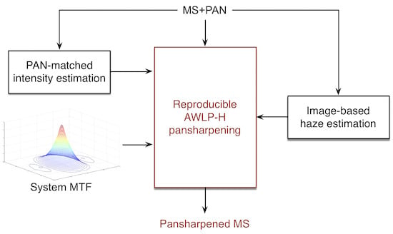
It is worth remarking that the proposed approach is optimized on both sensor and atmosphere. Indeed, the spatial response of the sensor is taken into account by the low-pass filter applied to ${\overline{\mathbf{P}}}^{\left({\tilde{\mathbf{M}}}_k\right)}$, which is designed to match the MTF of the MS sensor (i.e., imposing a Gaussian shape filter matched with the MS sensor’s MTF by fixing the gain at Nyquist frequency to $0.3$). Instead, the spectral response is implicitly considered when the weights to calculate the intensity component ${\widehat{\mathbf{I}}}_L$ are estimated according to the linear model in Equation (3). Finally, the atmospheric optimization is performed by considering the path radiance in the proposed haze-corrected AWLP method.

The image-based dark-object subtraction (DOS) method [35] is exploited for estimating the haze (atmospheric path-radiance) for each MS spectral band. Under the assumption that dark pixels exist within an image and have zero reflectance (or 1% reflectance), the radiance obtained by such dark pixels is mainly due to atmospheric path radiance [35]. Thus, the estimation of the coefficient $H_k$ for the k-th spectral band is performed by calculating the minimum of the k-th MS spectral band [28]. Thus, Equation (16) requires no parametric adjustments to find the values of haze.

5. Assessment Protocols and Indices

The assessment of pansharpening products is surely a critical issue [34]. Two validation procedures are often applied. The first one is the so-called validation at reduced scale [49]. It relies upon the reduction, through spatial filters, of the spatial resolution of both the MS and the Pan images aiming of exploiting the original MS image as reference [49]. In order to compare the fused product with the reference image, multidimensional indexes are used. In particular, the relative dimensionless global error in synthesis, ERGAS [1,34], the spectral angle mapper (SAM) [2], and the multispectral extension of the universal image quality index, generally called Q$2^n$ (Q4 for four bands and Q8 in the case of eight-band products) [50,51] are used in this work.

Despite of its accuracy (thanks to the presence of a reference image), the above-mentioned procedure is based on an implicit assumption of “invariance among scale” that could not be valid. For this reason, several protocols at full resolution, i.e., validating the fused products coming from the fusion of the original MS and PAN images, have been proposed in the literature [52,53,54,55,56,57]. In this work, the hybrid quality with no reference index (HQNR) [58] is selected. It consists of two indexes measuring the spatial distortion, $D_S$, borrowed by the one used in the QNR index [59], and the spectral distortion, $D_{\lambda }^{\left(K\right)}$, borrowed by the one of Khan’s protocol [60]. The HQNR is obtained by combining both the distortion indexes as follows:

$$\mathrm{HQNR}\triangleq {\left(1-D_{\lambda }^{\left(K\right)}\right)}^{\alpha }·{\left(1-D_S\right)}^{\beta }.$$

(17)

where $\alpha$ and $\beta$ are two coefficients that weight the spectral and the spatial contributions, respectively. Both the coefficients are set to 1. The two distortion indexes $D_{\lambda }^{\left(K\right)}$ and $D_S$ range from 0 to 1, thus even the HQNR can assume a value in the set $[0,1]$. Its ideal value is 1.

6. Experimental Results

The goal of this section is to perform a comprehensive and fair evaluation of the revisited AWLP pansharpening method, namely AWLP-H. Experiments have been carried out on real datasets acquired by three different satellite instruments over different landscapes. Evaluations are at degraded scale for all datasets and also at full scale for the 8-bands WorldView-2 dataset, more challenging and up-to-date, due to the higher number of bands and the presence of an upgradable operating constellation of satellites (WorldView-2/-3/-4, so far).

6.1. Datasets

• Toulouse dataset: An IKONOS image composed by 512×512 MS pixels and 2048×2048 panchromatic pixels has been acquired over the urban area of Toulouse, France, in June 2000. The MS sensor acquires four spectral bands in the visible and near-infrared (VNIR) spectrum range (i.e., blue, green, red, and near-infrared). The spatial sampling interval (SSI) is 4 m for the MS bands and 1 m for the Pan channel (the scale ratio R is equal to 4). The format of the data is spectral radiance rescaled to digital numbers (DNs) with 11-bits wordlength. A true color representation of the dataset is given in Figure 5l.
• Trento dataset: A QuickBird image composed by 256×256 MS pixels and 1024×1024 Pan pixels has been acquired over the outskirts of Trento, in Italy. The MS sensor acquires four spectral bands in the VNIR spectrum range (i.e., blue, green, red, and near-infrared). The SSI is $2.8$ m for MS and $0.7$ m for the Pan channel ($R=4$). The data format is spectral radiance rescaled to DNs with 11-bits resolution. A true color representation of the dataset is given in Figure 6l.
• Rio dataset: A WorldView-2 image composed by 512×512 MS pixels and 2048×2048 Pan pixels has been acquired over the urban area of Rio De Janeiro, in Brazil. The MS instrument acquires eight spectral bands in the VNIR spectrum range (i.e., coastal, blue, green, yellow, red, red edge, NIR1 and NIR2). The SSI is 2 m for MS and $0.5$ m for the Pan channel ($R=4$). The data format is spectral radiance rescaled to 11-bit DNs. A true color representation of the dataset is given in Figure 7l.

6.2. Methods

The benchmarks consist of several CS and MRA methods, mostly taken from the MS Pansharpening Toolbox [32]. The haze corrected versions of pure CS and MRA methods are taken from [29].

• EXP: the MS image interpolation using a polynomial kernel with 23 coefficients (EXP) [61];
• GS: Gram-Schmidt spectral sharpening [62] (Toolbox implementation [2]);
• GSA: GS with adaptive calculation of intensity [18] (Toolbox implementation [2]);
• BDSD: Band-dependent spatial detail [63] (Toolbox implementation [2]);
• MTF-GLP-CBD: MRA-based method with MTF-shaped analysis filters [19] with amplitude at Nyquist 0.25, generalized Laplacian pyramid decomposition and detail injection model based on projection (Toolbox implementation [2]);
• AWLP-Otazu: original implementation by X. Otazu et al. [31] (see Equation (11));
• AWLP-Toolbox: Toolbox implementation [2] of AWLP following the guidelines of [15] (see Equation (12));
• OBT-H: optimized Brovey transform with regression-based intensity component and contrast-based detail injection model with haze correction [29] (see Equation (14));
• MTF-GLP-HPM-H: MRA-based method with MTF filters, GLP analysis, and contrast-based detail injection model with haze correction [29];
• AWLP-H: AWLP-Toolbox with haze correction (see Equation (16)).

Furthermore, GT is the ground-truth (reference) image, only available for the reduced resolution test cases. It is worth remarking that the MTF-GLP-CBD, the BDSD, and the MTF-GLP-HPM-H methods exploit the knowledge of the sensor’s MTF. Instead, the other approaches in the benchmark do not use this a prior information. This can be considered as a further classification of the pansharpening approaches [64].

6.3. Fusion Simulations

A series of simulations at reduced scale has been performed.

Table 1. Degraded-resolution IKONOS Toulouse dataset: cumulative distortion and quality indexes. Best results in boldface; second best in italic.

	SAM	ERGAS	Q4
EXP	4.8403	5.8793	0.5185
GS	4.2603	4.1908	0.8082
GSA	3.0211	2.5860	0.9324
BDSD	2.7998	2.4674	0.9307
MTF-GLP-CBD	3.0159	2.5660	0.9332
AWLP-Otazu	4.8403	3.2624	0.8970
AWLP-Toolbox	3.6653	2.8281	0.9320
OBT-H	2.7713	2.4578	0.9350
MTF-GLP-HPM-H	2.7428	2.3884	0.9380
AWLP-H	2.7556	2.4330	0.9360
GT	0	0	1

,

Table 2. Degraded-resolution QuickBird Trento dataset: cumulative distortion and quality indexes. Best results in boldface; second best in italic.

	SAM	ERGAS	Q4
EXP	4.3152	4.6769	0.7600
GS	5.2356	4.1871	0.7994
GSA	4.6799	3.3997	0.8573
BDSD	4.3415	3.1802	0.8742
MTF-GLP-CBD	4.4858	3.1825	0.8690
AWLP-Otazu	4.3152	3.2195	0.8562
AWLP-Toolbox	3.9893	3.0819	0.8800
OBT-H	3.3547	2.8671	0.9086
MTF-GLP-HPM-H	3.3207	2.7351	0.9147
AWLP-H	3.3030	2.7162	0.9148
GT	0	0	1

and

Table 3. Degraded-resolution WorldView-2 Rio dataset: cumulative distortion and quality indexes. Best results in boldface; second best in italic.

	SAM	ERGAS	Q8
EXP	5.0695	6.3837	0.7245
GS	5.0822	4.1997	0.8607
GSA	4.3747	3.3158	0.9153
BDSD	4.8990	3.6592	0.8974
MTF-GLP-CBD	4.3274	3.2779	0.9198
AWLP-Otazu	5.0695	3.4988	0.9059
AWLP-Toolbox	4.6716	3.5206	0.9154
OBT-H	4.0205	3.1933	0.9215
MTF-GLP-HPM-H	3.9895	3.1504	0.9241
AWLP-H	4.0022	3.1602	0.9243
GT	0	0	1

show the quantitative assessment for the three datasets. The best performance for all the quality metrics is shared by the proposed AWLP-H and by MTF-GLP-HPM-H. Not surprisingly, because the two methods only differ by the denominator of the injection gain: ${\widehat{\mathbf{I}}}_L-H_p$, for the former, ${\overline{\mathbf{P}}}_L^{\left({\tilde{\mathbf{M}}}_k\right)}-H_p$, for the latter. In particular, a significant reduction in the SAM index can be observed with respect to the plain AWLP, which clamps the angle error of the interpolated image (EXP). This is further corroborated by the qualitative analysis of the pansharpened products in Figure 5, Figure 6 and Figure 7. While the spectral distortions of some products are noticeable, see, e.g., GS in Figure 5c and AWLP-Otazu in Figure 5g, the improved versions, GSA in Figure 5d and AWLP-H in Figure 5h, are much more similar to the GT (Figure 5l).

When the comparison is moved towards a more vegetated scenario, the Trento dataset, all methods except the haze-corrected versions, OBT-H, MTG-GLP-HPM-H and the proposed AWLP-H, suffer from a noticeable over-enhancement of vegetation due to textures of Pan injected into the B band [30], see the band analysis provided in

Table 4. Degraded-resolution QuickBird Trento dataset: Q-indexes for each spectral band, where $B1$, $B2$, $B3$, and $B4$ are the blue, the green, the red, and the NIR bands, respectively. The Q${}_{ave}$ column represents the averaged values. Best results in boldface; second best in italic.

	Q${}_{\mathit{B}1}$	Q${}_{\mathit{B}2}$	Q${}_{\mathit{B}3}$	Q${}_{\mathit{B}4}$	Q${}_{\mathit{a}\mathit{v}\mathit{e}}$
EXP	0.7883	0.7810	0.7906	0.7454	0.7764
GS	0.7836	0.8382	0.8235	0.8469	0.8231
GSA	0.8138	0.8652	0.8542	0.9077	0.8602
BDSD	0.8492	0.8864	0.8745	0.9211	0.8828
MTF-GLP-CBD	0.8296	0.8785	0.8649	0.9154	0.8721
AWLP-Otazu	0.7544	0.8832	0.9141	0.9334	0.8713
AWLP-Toolbox	0.8422	0.8654	0.9112	0.9318	0.8877
OBT-H	0.8982	0.9249	0.9184	0.9268	0.9171
MTF-GLP-HPM-H	0.9032	0.9305	0.9238	0.9352	0.9232
AWLP-H	0.9039	0.9308	0.9238	0.9349	0.9233
GT	1	1	1	1	1

where the Q-indexes of the blue band are high only for the haze-corrected methods. It is easy to note that rural areas are better represented by haze-corrected approaches, see the close-ups in Figure 8. Indeed, without any correction, the texture of the canopies, which are clear visible in the Pan image, are included in the pansharpened products as blueish texture due to the fact that the blue band is the one that exhibits the biggest path radiance in the visible spectrum. For the remaining areas (i.e., the urban ones), all the approaches get good performance. It is noteworthy that on this dataset, AWLP-H produces the best scores.

Same considerations apply to the visual assessment of the Rio dataset in Figure 7. In this case, however, the limited amount of vegetated area and the small overlap of Pan with the NIR1 band make the synthesis accuracy of vegetation less evident. The numerical values of the scores still highlight the superiority of the haze-corrected methods, in general, and of AWLP-H over its baseline, in particular, AWLP-Otazu.

Finally, the computational analysis has been performed on the degraded-resolution QuickBird Trento dataset, see

Table 5. Execution times of the pansharpening algorithms for the degraded-resolution QuickBird Trento dataset, run over an Intel(R) Core(TM) i7-7700HQ @2.80 GHz processor. The increments with respect to the fastest approach (i.e., GS) are also reported.

Method	Time [s]	Increment with Respect to GS
GS	0.04	0%
GSA	0.10	150%
BDSD	0.11	175%
MTF-GLP-CBD	0.09	125%
OBT-H	0.04	0%
MTF-GLP-HPM-H	0.18	350%
AWLP-Otazu	0.23	475%
AWLP-Toolbox	0.26	550%
AWLP-H	0.11	175%

. In particular, the computational times of the pansharpening algorithms have been calculated together with their increments with respect to the fastest method (i.e., the GS). It is clear to see that the proposed AWLP-H approach is faster than the other AWLPs with a strong reduction of the computational times. This assessment at reduced resolution demonstrates that the proposed approach is both fast and high performing.

An experiment of fusion at full scale has been carried out on the Rio dataset only. In fact, while IKONOS and QuickBird represent the past of VHR satellite MS scanners and may be of interest nowadays only for the historical series of data that have been collected, the three-satellites WorldView constellation is the present and near future of VHR spectral imaging from space. Numerical scores according to the HQNR index and its spectral and spatial components are reported in

Table 6. Full-scale Khan’s spectral distortion index, QNR spatial distortion index and cumulative score HQNR calculated on the 2048×2048 pansharpened WorldView-2 Rio image in Figure 9. Best results in boldface; second best in italic.

	${\mathit{D}}_{\mathit{\lambda }}^{\left(\mathit{K}\right)}$	${\mathit{D}}_{\mathit{S}}$	HQNR
EXP	0.0316	0.1963	0.7783
GS	0.0638	0.0908	0.8512
GSA	0.0321	0.1113	0.8601
BDSD	0.0401	0.0584	0.9039
MTF-GLP-CBD	0.0134	0.0955	0.8924
AWLP-Otazu	0.0224	0.0943	0.8854
AWLP-Toolbox	0.0227	0.0898	0.8896
OBT-H	0.0323	0.0895	0.8811
MTF-GLP-HPM-H	0.0154	0.0750	0.9107
AWLP-H	0.0145	0.0744	0.9122

for all the methods considered, with the obvious exception of GT. The benefits of the path-radiance correction are evident in term of decrements in both spectral and spatial distortions, as measured according to the spectral and spatial distortion indices, $D_{\lambda }^{\left(K\right)}$ and $D_S$, respectively. HQNR detects an improvement of the haze-corrected versions that are based on MRA, as substantially also a hybrid method like AWLP behaves. All pure CS-based methods, GS, GSA, BDSD and OBT-H, suffer from a spectral distortion almost twice that of MRA-based methods. This is presumably due to the slight local misregistration between interpolated MS and Pan [44], which is negligible in tests at degraded scale, where residual shifts are reduced by the spatial scale ratio: CS methods shift the fusion product towards Pan, thereby introducing a spatial mismatch with the original MS, which is the reference for the measurement of full-scale spectral quality, according to Wald’s protocol. While the most spatially accurate method is BDSD, followed by AWLP-H and MTF-GLP-HPM-H, the cumulative global index HQNR ranks AWLP-H, closely followed by MTF-GLP-HPM-H, as the most performing methods among those compared at full scale. Figure 9 shows the full-scale fusion products for all the nine methods considered. In the absence of a GT, the textured vegetation produced by GS, GSA, and AWLP-Otazu can appear as an asset, while AWLP-H is realistically less textured. There is no perceivable color distortion of GS over GSA and of AWLP-Otazu over AWLP-H. All methods seem to comparably perform. This behavior stresses the crucial concept that without statistical indices, but only with visual assessments, there would not have been progresses in pansharpening over the last twenty years (i.e., the time interval between GS and AWLP-H).

6.4. Discussion

Before the closing section, we wish to discuss quality issues relating MS images before and after pansharpening fusion. The quality of the original MS (and Pan) images can be described in terms of spectral, spatial (or geometric), and radiometric (or SNR) quality. Spectral quality is related to the SRFs of the instrument (see Figure 4) and is generally higher when the MS channels are narrow and little overlapped. In this sense, an HS image generally has greater spectral quality than an MS image. Spatial quality is related to the MTFs of the individual channels; the higher the MTF value at Nyquist, the higher the spatial sharpness and the geometrical accuracy of details. Radiometric quality is uniquely related to the photon and electronic noise of the instrument [65] and is usually measured as SNR. Spatial and radiometric quality issues apply also to the panchromatic channel.

Upon these premises, we wish to draw some guidelines to ensure that the pansharpened image has spectral, spatial, and radiometric qualities comparable with those of the original MS and Pan datasets. The check of the consistency property of Wald’s protocol ensures that the spectral quality of the pansharpened product is comparable with that of the original MS data. In other words, if a fusion method does not mix the low-pass frequency components of the MS image with those of Pan, the spectral quality is retained. The spatial quality (MTF) of the fusion product is arguably the MTF of enhancing Pan. So, if the MTF of the original MS is, say, 0.3 and the MTF of Pan is 0.2, then the MTF of the pansharpened product will be much closer to 0.2 than to 0.3. This explains why in fusion simulations at degraded scale, the MTF-like filter used to degrade the Pan image is taken equal to the widest of the MTFs of the original MS bands. Eventually, the radiometric quality would imply that the SNR of the pansharpened MS bands is not lower than that of the original MS bands. This is possible only if the Pan image has SNR greater than that of the MS bands. This issue has motivated the use of the time delay integration (TDI) technique, especially for Pan; more recently, and to a lower extent, also for MS, to ensure that the SNR of Pan is always greater than that of MS channels.

7. Conclusions

In this study, we pointed out the need for a fast and high performing pansharpening method providing reproducible results on any dataset of any size. Such a method, on one side, should expedite routine fusion of large datasets (e.g., Google Earth), on the other side, should become an essential tool for a fair benchmarking of newly developed methods. Starting from a popular hybrid method developed in 2005, a series of modifications has been introduced to achieve an implicit optimization towards the spectral and spatial responses of the imaging instrument and towards the radiative transfer through the atmosphere.

The spectral response is captured by a multivariate regression of the interpolated MS bands providing an intensity component that is least squares-matched to a low-pass version of the Pan image. The spatial response is accounted by using Gaussian-like analysis filters matched with the MTF of the MS channels that is a solution widely established in the literature. Eventually, the imaging mechanism through the atmosphere is exploited through a correction in the multiplicative detail-injection model of MS path-radiance terms, estimated by means of the dark-object image-based method, as the minimum values attained over each spectral band. In fact, estimation and correction of path-radiances are relevant to get high performance from pansharpening methods relied upon spatial modulation.

The proposed AWLP with haze-correction, referred to as AWLP-H, is fast and comparable, from a computational point of view, with classical methods (see, e.g., the GS). Nevertheless, AWLP-H achieves the best performance among the most powerful methods of the Pansharpening Toolbox [2] in a fair and reproducible assessment, carried out both at reduced and at full scale, on three different datasets from as many instruments. The procedure does not need any adjustments for WorldView data, i.e., where some MS bands do not overlap with the Pan channel.

References

- Alparone, L.; Aiazzi, B.; Baronti, S.; Garzelli, A. Remote Sensing Image Fusion; CRC Press: Boca Raton, FL, USA, 2015. [Google Scholar]
- Vivone, G.; Alparone, L.; Chanussot, J.; Dalla Mura, M.; Garzelli, A.; Licciardi, G.A.; Restaino, R.; Wald, L. A critical comparison among pansharpening algorithms. IEEE Trans. Geosci. Remote Sens. 2015, 53, 2565–2586. [Google Scholar] [CrossRef]
- Li, Z.; Zhang, H.K.; Roy, D.P.; Yan, L.; Huang, H.; Li, J. Landsat 15-m panchromatic-assisted downscaling (LPAD) of the 30-m reflective wavelength bands to Sentinel-2 20-m resolution. Remote Sens. 2017, 9, 755. [Google Scholar]
- Selva, M.; Aiazzi, B.; Butera, F.; Chiarantini, L.; Baronti, S. Hyper-sharpening: A first approach on SIM-GA data. IEEE J. Sel. Top. Appl. Earth Observ. Remote Sens. 2015, 8, 3008–3024. [Google Scholar] [CrossRef]
- Selva, M.; Santurri, L.; Baronti, S. Improving hypersharpening for WorldView-3 data. IEEE Geosci. Remote Sens. Lett. 2019, 16, 987–991. [Google Scholar] [CrossRef]
- Yin, H. A joint sparse and low-rank decomposition for pansharpening of multispectral images. IEEE Trans. Geosci. Remote Sens. 2017, 55, 3545–3557. [Google Scholar] [CrossRef]
- Garzelli, A. A review of image fusion algorithms based on the super-resolution paradigm. Remote Sens. 2016, 8, 797. [Google Scholar] [CrossRef]
- Meng, X.; Shen, H.; Li, H.; Zhang, L.; Fu, R. Review of the pansharpening methods for remote sensing images based on the idea of meta-analysis. Inform. Fusion 2019, 46, 102–113. [Google Scholar] [CrossRef]
- Zhu, X.X.; Grohnfeld, C.; Bamler, R. Exploiting joint sparsity for pan-sharpening: The J-sparseFI algorithm. IEEE Trans. Geosci. Remote Sens. 2016, 54, 2664–2681. [Google Scholar] [CrossRef]
- Palsson, F.; Sveinsson, J.R.; Ulfarsson, M.O. A new pansharpening algorithm based on total variation. IEEE Geosci. Remote Sens. Lett. 2014, 11, 318–322. [Google Scholar] [CrossRef]
- Addesso, P.; Longo, M.; Restaino, R.; Vivone, G. Sequential Bayesian methods for resolution enhancement of TIR image sequences. IEEE J. Sel. Top. Appl. Earth Observ. Remote Sens. 2015, 8, 233–243. [Google Scholar] [CrossRef]
- Scarpa, G.; Vitale, S.; Cozzolino, D. Target-adaptive CNN-based pansharpening. IEEE Trans. Geosci. Remote Sens. 2018, 56, 5443–5457. [Google Scholar] [CrossRef]
- Chavez, P.S., Jr.; Sides, S.C.; Anderson, J.A. Comparison of three different methods to merge multiresolution and multispectral data: Landsat TM and SPOT panchromatic. Photogramm. Eng. Remote Sens. 1991, 57, 295–303. [Google Scholar]
- Alparone, L.; Aiazzi, B.; Baronti, S.; Garzelli, A. Spatial methods for multispectral pansharpening: Multiresolution analysis demystified. IEEE Trans. Geosci. Remote Sens. 2016, 54, 2563–2576. [Google Scholar] [CrossRef]
- Alparone, L.; Garzelli, A.; Vivone, G. Intersensor statistical matching for pansharpening: Theoretical issues and practical solutions. IEEE Trans. Geosci. Remote Sens. 2017, 55, 4682–4695. [Google Scholar] [CrossRef]
- Xie, B.; Zhang, H.K.; Huang, B. Revealing implicit assumptions of the component substitution pansharpening methods. Remote Sens. 2017, 9, 443. [Google Scholar] [CrossRef]
- Vivone, G.; Restaino, R.; Chanussot, J. A regression-based high-pass modulation pansharpening approach. IEEE Trans. Geosci. Remote Sens. 2018, 56, 984–996. [Google Scholar] [CrossRef]
- Aiazzi, B.; Baronti, S.; Selva, M. Improving component substitution pansharpening through multivariate regression of MS+Pan data. IEEE Trans. Geosci. Remote Sens. 2007, 45, 3230–3239. [Google Scholar] [CrossRef]
- Aiazzi, B.; Alparone, L.; Baronti, S.; Garzelli, A.; Selva, M. MTF-tailored multiscale fusion of high-resolution MS and Pan imagery. Photogramm. Eng. Remote Sens. 2006, 72, 591–596. [Google Scholar] [CrossRef]
- Vivone, G.; Restaino, R.; Chanussot, J. Full scale regression-based injection coefficients for panchromatic sharpening. IEEE Trans. Image Process. 2018, 27, 3418–3431. [Google Scholar] [CrossRef]
- Aiazzi, B.; Baronti, S.; Lotti, F.; Selva, M. A comparison between global and context-adaptive pansharpening of multispectral images. IEEE Geosci. Remote Sens. Lett. 2009, 6, 302–306. [Google Scholar] [CrossRef]
- Liu, J.G. Smoothing filter based intensity modulation: A spectral preserve image fusion technique for improving spatial details. Int. J. Remote Sens. 2000, 21, 3461–3472. [Google Scholar] [CrossRef]
- Alparone, L.; Aiazzi, B.; Baronti, S.; Garzelli, A. Sharpening of very high resolution images with spectral distortion minimization. Proc. IEEE Int. Geosci. Remote Sens. Symp. 2003, 1, 458–460. [Google Scholar]
- Garzelli, A. Wavelet-based fusion of optical and SAR image data over urban area. ISPRS Arch. 2002, 34, 59–62. [Google Scholar]
- Alparone, L.; Facheris, L.; Baronti, S.; Garzelli, A.; Nencini, F. Fusion of multispectral and SAR images by intensity modulation. In Proceedings of the 7th International Conference on Information Fusion, Stockholm, Sweden, 28 June–1 July 2004; Volume 2, pp. 637–643. [Google Scholar]
- Pacifici, F.; Longbotham, N.; Emery, W.J. The importance of physical quantities for the analysis of multitemporal and multiangular optical very high spatial resolution images. IEEE Trans. Geosci. Remote Sens. 2014, 52, 6241–6256. [Google Scholar] [CrossRef]
- Schowengerdt, R.A. Remote Sensing: Models and Methods for Image Processing, 2nd ed.; Academic Press: Orlando, FL, USA, 1997. [Google Scholar]
- Li, H.; Jing, L. Improvement of a pansharpening method taking into account haze. IEEE J. Sel. Top. Appl. Earth Observ. Remote Sens. 2017, 10, 5039–5055. [Google Scholar] [CrossRef]
- Lolli, S.; Alparone, L.; Garzelli, A.; Vivone, G. Haze correction for contrast-based multispectral pansharpening. IEEE Geosci. Remote Sens. Lett. 2017, 14, 2255–2259. [Google Scholar] [CrossRef]
- Garzelli, A.; Aiazzi, B.; Alparone, L.; Lolli, S.; Vivone, G. Multispectral pansharpening with radiative transfer-based detail-injection modeling for preserving changes in vegetation cover. Remote Sens. 2018, 10, 1308. [Google Scholar] [CrossRef]
- Otazu, X.; González-Audícana, M.; Fors, O.; Núñez, J. Introduction of sensor spectral response into image fusion methods. Application to wavelet-based methods. IEEE Trans. Geosci. Remote Sens. 2005, 43, 2376–2385. [Google Scholar] [CrossRef] [Green Version]
- Vivone, G.; Alparone, L.; Chanussot, J.; Dalla Mura, M.; Garzelli, A.; Licciardi, G.A.; Restaino, R.; Wald, L. A critical comparison of pansharpening algorithms. In Proceedings of the 2014 IEEE Geoscience and Remote Sensing Symposium, Quebec City, QC, Canada, 13–18 July 2014; pp. 191–194. [Google Scholar]
- Coppo, P.; Chiarantini, L.; Alparone, L. End-to-end image simulator for optical imaging systems: Equations and simulation examples. Adv. Opt. Technol. 2013, 2013. [Google Scholar] [CrossRef]
- Thomas, C.; Ranchin, T.; Wald, L.; Chanussot, J. Synthesis of multispectral images to high spatial resolution: A critical review of fusion methods based on remote sensing physics. IEEE Trans. Geosci. Remote Sens. 2008, 46, 1301–1312. [Google Scholar] [CrossRef]
- Chavez, P.S., Jr. An improved dark-object subtraction technique for atmospheric scattering correction of multispectral data. Remote Sens. Environ. 1988, 24, 459–479. [Google Scholar] [CrossRef]
- Chavez, P.S., Jr. Image-based atmospheric corrections–Revisited and improved. Photogramm. Eng. Remote Sens. 1996, 62, 1025–1036. [Google Scholar]
- Lolli, S.; Di Girolamo, P.; Demoz, B.; Li, X.; Welton, E. Rain evaporation rate estimates from dual-wavelength lidar measurements and intercomparison against a model analytical solution. J. Atmos. Ocean. Technol. 2017, 34, 829–839. [Google Scholar] [CrossRef]
- Alparone, L.; Selva, M.; Aiazzi, B.; Baronti, S.; Butera, F.; Chiarantini, L. Signal-dependent noise modelling and estimation of new-generation imaging spectrometers. In Proceedings of the 2009 First Workshop on Hyperspectral Image and Signal Processing: Evolution in Remote Sensing, Grenoble, France, 26–28 August 2009. [Google Scholar]
- Lolli, S.; Delaval, A.; Loth, C.; Garnier, A.; Flamant, P. 0.355-micrometer direct detection wind lidar under testing during a field campaign in consideration of ESA’s ADM-Aeolus mission. Atmos. Meas. Tech. 2013, 6, 3349–3358. [Google Scholar] [CrossRef]
- Campbell, J.; Ge, C.; Wang, J.; Welton, E.; Bucholtz, A.; Hyer, E.; Reid, E.; Chew, B.; Liew, S.C.; Salinas, S.; et al. Applying advanced ground-based remote sensing in the Southeast Asian maritime continent to characterize regional proficiencies in smoke transport modeling. J. Appl. Meteorol. Climatol. 2016, 55, 3–22. [Google Scholar] [CrossRef]
- Lolli, S.; Campbell, J.; Lewis, J.; Gu, Y.; Marquis, J.; Chew, B.; Liew, S.C.; Salinas, S.; Welton, E. Daytime top-of-the-atmosphere cirrus cloud radiative forcing properties at Singapore. J. Appl. Meteorol. Climatol. 2017, 56, 1249–1257. [Google Scholar] [CrossRef]
- Lolli, S.; Madonna, F.; Rosoldi, M.; Campbell, J.R.; Welton, E.J.; Lewis, J.R.; Gu, Y.; Pappalardo, G. Impact of varying lidar measurement and data processing techniques in evaluating cirrus cloud and aerosol direct radiative effects. Atmos. Meas. Tech. 2018, 11, 1639–1651. [Google Scholar] [CrossRef] [Green Version]
- Fu, Q.; Liou, K.N. On the correlated k-distribution method for radiative transfer in nonhomogeneous atmospheres. J. Atmos. Sci. 1992, 49, 2139–2156. [Google Scholar] [CrossRef]
- Aiazzi, B.; Alparone, L.; Garzelli, A.; Santurri, L. Blind correction of local misalignments between multispectral and panchromatic images. IEEE Geosci. Remote Sens. Lett. 2018, 15, 1625–1629. [Google Scholar] [CrossRef]
- Baronti, S.; Aiazzi, B.; Selva, M.; Garzelli, A.; Alparone, L. A theoretical analysis of the effects of aliasing and misregistration on pansharpened imagery. IEEE J. Sel. Top. Signal Process. 2011, 5, 446–453. [Google Scholar] [CrossRef]
- Aiazzi, B.; Alparone, L.; Baronti, S.; Carlà, R.; Garzelli, A.; Santurri, L. Sensitivity of pansharpening methods to temporal and instrumental changes between multispectral and panchromatic data sets. IEEE Trans. Geosci. Remote Sens. 2017, 55, 308–319. [Google Scholar] [CrossRef]
- Shah, V.P.; Younan, N.H.; King, R.L. An efficient pan-sharpening method via a combined adaptive-PCA approach and contourlets. IEEE Trans. Geosci. Remote Sens. 2008, 46, 1323–1335. [Google Scholar] [CrossRef]
- Licciardi, G.A.; Khan, M.M.; Chanussot, J. Fusion of hyperspectral and panchromatic images: A hybrid use of indusion and nonlinear PCA. In Proceedings of the 2012 19th IEEE International Conference on Image Processing, Orlando, FL, USA, 30 September–3 October 2012; pp. 2133–2136. [Google Scholar]
- Wald, L.; Ranchin, T.; Mangolini, M. Fusion of satellite images of different spatial resolutions: Assessing the quality of resulting images. Photogramm. Eng. Remote Sens. 1997, 63, 691–699. [Google Scholar]
- Alparone, L.; Baronti, S.; Garzelli, A.; Nencini, F. A global quality measurement of pan-sharpened multispectral imagery. IEEE Geosci. Remote Sens. Lett. 2004, 1, 313–317. [Google Scholar] [CrossRef]
- Garzelli, A.; Nencini, F. Hypercomplex quality assessment of multi-/hyper-spectral images. IEEE Geosci. Remote Sens. Lett. 2009, 6, 662–665. [Google Scholar] [CrossRef]
- Aiazzi, B.; Alparone, L.; Baronti, S.; Carlà, R. Assessment of pyramid-based multisensor image data fusion. In Image and Signal Processing for Remote Sensing IV; Serpico, S.B., Ed.; International Society for Optics and Photonics: Barcelona, Spain, 1998; pp. 237–248. [Google Scholar]
- Aiazzi, B.; Alparone, L.; Argenti, F.; Baronti, S. Wavelet and pyramid techniques for multisensor data fusion: A performance comparison varying with scale ratios. In Image and Signal Processing for Remote Sensing V; Serpico, S.B., Ed.; International Society for Optics and Photonics: Florence, Italy, 1999; pp. 251–262. [Google Scholar]
- Du, Q.; Younan, N.H.; King, R.L.; Shah, V.P. On the performance evaluation of pan-sharpening techniques. IEEE Geosci. Remote Sens. Lett. 2007, 4, 518–522. [Google Scholar] [CrossRef]
- Carlà, R.; Santurri, L.; Aiazzi, B.; Baronti, S. Full-scale assessment of pansharpening through polynomial fitting of multiscale measurements. IEEE Trans. Geosci. Remote Sens. 2015, 53, 6344–6355. [Google Scholar] [CrossRef]
- Vivone, G.; Restaino, R.; Chanussot, J. A Bayesian procedure for full resolution quality assessment of pansharpened products. IEEE Trans. Geosci. Remote Sens. 2018, 56, 4820–4834. [Google Scholar] [CrossRef]
- Selva, M.; Santurri, L.; Baronti, S. On the use of the expanded image in quality assessment of pansharpened images. IEEE Geosci. Remote Sens. Lett. 2018, 15, 320–324. [Google Scholar] [CrossRef]
- Aiazzi, B.; Alparone, L.; Baronti, S.; Carlà, R.; Garzelli, A.; Santurri, L. Full scale assessment of pansharpening methods and data products. In Image and Signal Processing for Remote Sensing XX; Bruzzone, L., Ed.; International Society for Optics and Photonics: Amsterdam, The Netherlands, 2014; p. 924402. [Google Scholar]
- Alparone, L.; Aiazzi, B.; Baronti, S.; Garzelli, A.; Nencini, F.; Selva, M. Multispectral and panchromatic data fusion assessment without reference. Photogramm. Eng. Remote Sens. 2008, 74, 193–200. [Google Scholar] [CrossRef]
- Khan, M.M.; Alparone, L.; Chanussot, J. Pansharpening quality assessment using the modulation transfer functions of instruments. IEEE Trans. Geosci. Remote Sens. 2009, 47, 3880–3891. [Google Scholar] [CrossRef]
- Aiazzi, B.; Baronti, S.; Selva, M.; Alparone, L. Bi-cubic interpolation for shift-free pan-sharpening. ISPRS J. Photogramm. Remote Sens. 2013, 86, 65–76. [Google Scholar] [CrossRef]
- Laben, C.A.; Brower, B.V. Process for Enhancing the Spatial Resolution of Multispectral Imagery Using Pan-Sharpening, 2000. U.S. Patent #6,011,875, 4 January 2000. [Google Scholar]
- Garzelli, A.; Nencini, F.; Capobianco, L. Optimal MMSE Pan sharpening of very high resolution multispectral images. IEEE Trans. Geosci. Remote Sens. 2008, 46, 228–236. [Google Scholar] [CrossRef]
- Kwan, C.; Choi, J.; Chan, S.; Zhou, J.; Budavari, B. A super-resolution and fusion approach to enhancing hyperspectral images. Remote Sens. 2018, 10, 1416. [Google Scholar] [CrossRef]
- Alparone, L.; Selva, M.; Capobianco, L.; Moretti, S.; Chiarantini, L.; Butera, F. Quality assessment of data products from a new generation airborne imaging spectrometer. Proc. IGARSS 2009, IV, IV422–IV425. [Google Scholar]
Figure 1.
Overview of the sensor’s acquisition model.
Figure 2.
Spatial frequency response of (a) ideal and (b) true multispectral (MS) scanners. The ideal modulation transfer function (MTF) depends only on the optics. The true MTF considers also along-track motion and vibrations of the satellite as well as finite sampling of detectors.
Figure 3.
MTFs typically used to model real sensors. These are Gaussian-shaped with magnitudes of 0.1, 0.2, and 0.3 at Nyquist frequency. The dashed line represents the spectrum of the Pan image, whose high-frequency content is selected by each high-pass filters designed starting from the knowledge of the sensors’ MTFs. The dotted vertical line marks the Nyquist frequency of MS, one fourth of the Nyquist frequency of Pan, which is half the sampling frequency of Pan (equal to one in normalized plots).
Figure 4.
Spectral responsivity functions of MS scanners: (a) IKONOS, (b) QuickBird, (c) GeoEye-1 (4-bands MS + Pan); (d) WorldView-2 (8-bands MS + Pan).
Figure 5.
Panchromatic and true-color compositions of 256×256 detail of 4 m degraded-scale pansharpened IKONOS Toulouse for the following methods: (a): Pan; (b): EXP; (c): GS; (d): GSA; (e): BDSD; (f): MTF-GLP-CBD; (g): AWLP-Otazu; (h): AWLP-Toolbox; (i): OBT-H; (j): MTF-GLP-HPM-H; (k): AWLP-H; (l): GT.
Figure 6.
Panchromatic and true-color compositions of 256×256 2.8 m degraded-scale pansharpened QuickBird Trento for the following methods: (a): Pan; (b): EXP; (c): GS; (d): GSA; (e): BDSD; (f): MTF-GLP-CBD; (g): AWLP-Otazu; (h): AWLP-Toolbox; (i): OBT-H; (j): MTF-GLP-HPM-H; (k): AWLP-H; (l): GT.
Figure 7.
Panchromatic and true-color compositions of 256×256 detail of 2 m degraded-scale pansharpened WorldView-2 Rio for the following methods: (a): Pan; (b): EXP; (c): GS; (d): GSA; (e): BDSD; (f): MTF-GLP-CBD; (g): AWLP-Otazu; (h): AWLP-Toolbox; (i): OBT-H; (j): MTF-GLP-HPM-H; (k): AWLP-H; (l): GT.
Figure 8.
Panchromatic and true-color close-ups of the 2.8 m degraded-scale pansharpened QuickBird Trento for the following methods: (a): Pan; (b): EXP; (c): GS; (d): GSA; (e): BDSD; (f): MTF-GLP-CBD; (g): AWLP-Otazu; (h): AWLP-Toolbox; (i): OBT-H; (j): MTF-GLP-HPM-H; (k): AWLP-H; (l): GT.
Figure 9.
True-color compositions of 512×512 details of 0.5 m full-scale pansharpened WorldView-2 Rio for the following methods: (a): GS; (b): GSA; (c): BDSD; (d): MTF-GLP-CBD; (e): AWLP-Otazu; (f): AWLP-Toolbox; (g): OBT-H; (h): MTF-GLP-HPM-H; (i): AWLP-H.