Sentinel-1 Data for Winter Wheat Phenology Monitoring and Mapping
by
 , , , , ,
Ali Nasrallah
1,2,3,* ,
,
Nicolas Baghdadi
1,
Mohammad El Hajj
1,
Talal Darwish
2,
Hatem Belhouchette
3, 
Ghaleb Faour
2,
Salem Darwich
4 and
Mario Mhawej
2 1
IRSTEA, University of Montpellier, TETIS, 34090 Montpellier, France
2
National Center for Remote Sensing, National Council for Scientific Research (CNRS), Riad al Soloh, Beirut 1107 2260, Lebanon
3
CIHEAM-IAMM, UMR-System, 34090 Montpellier, France
4
Faculty of Agriculture, Lebanese University, Beirut 99, Lebanon
*
Author to whom correspondence should be addressed.
Remote Sens. 2019, 11(19), 2228; https://doi.org/10.3390/rs11192228
Submission received: 19 August 2019
/
Revised: 18 September 2019
/
Accepted: 23 September 2019
/
Published: 25 September 2019
(This article belongs to the Special Issue Remote Sensing: 10th Anniversary)
Abstract
:The ability of Synthetic Aperture Radar (SAR) Sentinel-1 data to detect the main wheat phenological phases was investigated in the Bekaa plain of Lebanon. Accordingly, the temporal variation of Sentinel-1 (S1) signal was analyzed as a function of the phenological phases’ dates observed in situ (germination; heading and soft dough), and harvesting. Results showed that S1 data, unlike the Normalized Difference Vegetation Index (NDVI) data, were able to estimate the dates of theses phenological phases due to significant variations in S1 temporal series at the dates of germination, heading, soft dough, and harvesting. Particularly, the ratio VV/VH at low incidence angle (32–34°) was able to detect the germination and harvesting dates. VV polarization at low incidence angle (32–34°) was able to detect the heading phase, while VH polarization at high incidence angle (43–45°) was better than that at low incidence angle (32–34°), in detecting the soft dough phase. An automated approach for main wheat phenological phases’ determination was then developed on the western part of the Bekaa plain. This approach modelled the S1 SAR temporal series by smoothing and fitting the temporal series with Gaussian functions (up to three Gaussians) allowing thus to automatically detect the main wheat phenological phases from the sum of these Gaussians. To test its robustness, the automated method was applied on the northern part of the Bekaa plain, in which winter wheat is harvested usually earlier because of the different weather conditions. The Root Mean Square Error (RMSE) of the estimation of the phenological phases’ dates was 2.9 days for germination, 5.5 days for heading, 5.1 days soft dough, 3.0 days for West Bekaa’s harvesting, and 4.5 days for North Bekaa’s harvesting. In addition, a slight underestimation was observed for germination and heading of West Bekaa (−0.2 and −1.1 days, respectively) while an overestimation was observed for soft dough of West Bekaa and harvesting for both West and North Bekaa (3.1, 0.6, and 3.6 days, respectively). These results are encouraging, and thus prove that S1 data are powerful as a tool for crop monitoring, to serve enhanced crop management and production handling.
1. Introduction
Demanding and achieving sufficient and stable crop productivity is a global desire. Crop management must be conscientious to climatic variability and adapt its practices to the given conditions, whether socio-economic oriented, or environmentally related. From this perspective, it is very important to understand the mechanisms driving the whole cropping cycle, to eventually understand the dynamics leading to attain each of its physiological phases [1]. The continuous identification of the phenological status of the crops is highly necessary, especially the phenological phases at which farmers’ and decision-makers’ interventions are required, speaking of irrigation, fertilization, pesticides application, and yield handling [1,2,3]. From this perspective, the original motivation of this paper comes from farming practices in winter wheat plots over semi-arid regions like the Bekaa plain of Lebanon. Globally, at a given winter wheat plot, germination is a very critical phase to be known, from which the future projection of the season can be made. From a modelling (crop simulation models) perspective, the germination is the very starting point to initiate the calculation of the growing degree days (GDD) accumulation, which is very important when known well, to properly estimate the whole seasonal phenology for best modelling (growth and production) outputs [4]. Because of the precipitation scarcity [5,6,7], supplementary irrigation is applied to wheat during spring to secure wheat water demands. Thus, the irrigation events take place between March and April, during the wheat vegetative cycle, which ends at heading/start of flowering. Applying late irrigation, however after this time (i.e., flowering) would lead to various consequences: (1) Reduced water use efficiency [8,9,10], (2) increased fungal diseases [11,12,13], and (3) stem lodging [13,14]. These consequences, nevertheless, will result in substantial reduction in the final wheat grain yield and/or in a lower net profit, putting the farmer at high economic risk. In regard to fertilizers applications, various studies have proven that nitrogen application could be either applied after sowing, and/or during the tillering time [15,16,17,18]. Thus, it is very important to note that when heading is reached, any added nitrogen would lead to nitrogen loss and low nitrogen-use efficiency, which will cause, beside the environmental consequences, a tremendous drop in the whole system efficiency and the final net profit. However, if the purpose is to increase the grain quality by enhancing the protein content, identifying heading is required to apply nitrogen at flowering phase [15,19]. Ultimately, wheat farmers apply their fungicides as the flag leaf starts appearing until it is fully expanded. When the flag leaf is fully expanded, heading phase had started and it is very critical that any fungicidal application should stop at this point [11,13]. At the soft dough phase, total maximum dry matter content and total nitrogen accumulation occur [20]. In addition, at soft dough phase, it is potentially feasible to predict the final grain protein content. The application of fungicides at earlier phases (during flag leaf expansion) aims to reduce the infection of wheat by fusarium head blight (FHB), which can be visually evaluated by carrying out visual observations during the soft dough phase, raising the importance of the identification of this phase for fast interventions [11,12]. Several studies, nevertheless, have stated that during very high temperatures after anthesis had taken place, applying irrigation in small amounts from flowering to soft dough phases could be desirable for maximizing the final grain yield [18,21]. In Mediterranean countries, where wheat is financially supported by subsidy system, the reception of the grains has to be done fast, to avoid further quality deterioration, as well as to support farmers with the required payments (based on areas or production). Thus, identifying harvesting time at plot scale is important as post-harvest handling of wheat grains could be very critical [22]. As storage period time increases, the risk of mycotoxins and fungus contamination increases and the need of grain fumigation during storage period would rise [23].
Intensive field work and in situ campaigns are known to require large number of personnel, high logistical supply, machinery and equipment, and thus huge budgets, which increase with the increasing area of the study site. In this context, remotely sensing data provide information on the spatial distribution [24] in addition to monitoring crop growth by providing precise and timely information on the phenological status and vegetation development. From field to global scale, remote sensing tools can tackle these information, especially when coupled with crop growth models for assessing crop yields [25,26,27,28] and computing their water cycle budgets [29,30,31,32].
By the route of vegetation indices, optical data (e.g., Sentinel-2, Landsat 8, and MODIS) have been widely used by seeking the interconnection between the plant optical properties and its photosynthetic activity characterized by the content of chlorophyll in the leaves [33]. Even though different vegetation indices have been developed and used (e.g., Enhanced Vegetation Index (EVI) [34] and the Soil Adjusted Vegetation Index (SAVI) [35]), the most used vegetation index is the Normalized Difference Vegetation Index (NDVI) [36], which has been directly related to the leaf area index (LAI) [35]. In their significant contribution, the optical satellites have been used for crop area estimates through the production of crop type maps and crop classification [37,38,39], and plant-biophysical related properties [40,41]. Apart from being limited by cloudy weather conditions, one limitation, however, in using NDVI resides in reaching saturation in dense vegetation canopies, resulting from the saturation of LAI for values above 3 m2/m2 (i.e., very low sensitivity of NDVI at high values of leaf area index) [42,43,44,45,46,47]. This may cause, nevertheless, uncertainty in detecting the crop physiological phases, and underestimation of ecosystem productivity in high (dense) biomass regions. With regard to Synthetic Aperture Radar (SAR), many studies have been carried out utilizing these data in their relation to crop classification [48], soil moisture estimations [49,50], and crop phenological trajectory interpretations [51,52]. Because of its complexity and interpretation difficulties, SAR data, however, have been less used in the agricultural field applications, compared to optical data.
By the launching of the first Sentinel satellite developed by the European Space Agency (ESA), free-of-charge data for the operational needs of the Copernicus program became available. From Sentinel-1A (April 2014) to Sentinel-1B (April 2016), C-band multi-temporal series of SAR imageries were made available at high spatial (10 m) and temporal (6 days) resolutions. While for optical data supply, Sentinel-2A and Sentinel-2B, developed by ESA as well, allow the availability of free high spatial (10 m) and temporal (5 days) resolutions data. The launching of Sentinel-2A and Sentinel-2B was in June 2015 and March 2017 respectively, as an integral part of Europe’s Copernicus program aiming at independent and continued global observation capacities [53]. As the planned continuity of Sentinel data until 2030 is ensured, the future generation of Sentinel imageries beyond 2030 is nonetheless planned. Hence, free and accurate continued crop monitoring will continue to exist. In regard to crop monitoring, minor number of studies have significantly relied on heavy time-series Sentinel-1 (SAR) data for monitoring different types of crops [48,54,55]. In order to come up with reliable outputs, understanding the physiological cycle of the studied crops is highly vital.
The paper focuses on the analysis of the temporal behavior of Sentinel-1 SAR backscatter coefficients (VV and VH) at two SAR incidence angles (32–34° and 43–45°) and of NDVI calculated from Sentinel-2 images of the wheat crop in the Bekaa plain of Lebanon. The main objective of the paper is to confirm that Sentienl-1 C-band data are able to identify spatially and temporally three winter wheat key phenological phases that are of high economic and agronomic importance, namely germination, heading and soft dough phases, in addition to harvesting. The successful identification and mapping of these phases reduce the economic losses on the farmer, as well as on the policymakers because of their direct relation to some agricultural practices in response to biotic or edaphic stresses on one hand, and to take care of the national grain production on the other. The paper is organized as material and methods (Section 2), presentation of main results (Section 3), discussion of the results (Section 4), and conclusions (Section 5).
2. Material and Methods
2.1. Study Site
The Bekaa plain of Lebanon, which is a flat valley, is the selected study area for this study. The plain, which is shown in Figure 1, is located between 33°33′ N and 34°00′ N latitude, 35°40′ E and 36°14′ E longitude covering an area of about 860 km2. The study region is located between two natural units having very steep slopes; the eastern slopes of the Mount-Lebanon Mountains (western unit) and the western slopes of the Anti-Lebanon Mountains (eastern unit). The study site is stretched from Baalbek (characterized by semi-arid climate) to the Qaraoun Lake (characterized by the Mediterranean climate). The average annual precipitation is around 600 mm. Economically, agriculture is the main activity securing the farmers’ livelihood at the plain [24,56]. Out of the main cultivated field crops, winter wheat and potato occupy the largest areas of cultivated arable lands [57]. In November, after the first effective rain, wheat farmers launch their sowing procedure to eventually harvest in June-July the year after, occupying up to 12,000 ha annually of the plain. Over 80% of the wheat plots are supplementary irrigated. The frequency of the irrigation occurrence is linked directly with the rainfall received during the season. However, as normally the rain stops in February-March, farmers tend to irrigate for the sake of better grain yield at the end of the season. Nitrogen is the other main input to wheat. The most growth driving nutrient (Nitrogen) is supplied by wheat farmers as ammonium sulfate in amounts of up to 230 Kg/ha. However, the amounts and timing vary among farmers because of different fertilization management practices, as well as the crop rotation types.
2.2. Remote Sensing Data
2.2.1. Optical Data
Fifty-eight optical images were acquired by the two twin satellites of Sentinel-2 (Sentinel-2A and Sentinel-2B). The acquired images cover a period from November 2017 to August 2018. The period corresponds to some period before sowing, the whole crop (i.e., winter wheat) cycle, and some period after harvesting the crop. The reason behind this is to make sure that the whole crop cycle is tracked on one hand, and to see whether there is any contribution of a previous and/or following crop, on the other. The pre-processing of L1C (Top of Atmosphere or TOA reflectance) Sentinel-2 images, which includes ortho-rectification, cloud removal (using cloud mask produced by Sen2Cor/SNAP), radiometric calibration, and atmospheric correction, was produced using SNAP/Sentinel-2 toolbox. The output of the pre-processing corresponded to L2A (bottom of atmosphere or BOA reflectance). The reason behind using the optical images (Sentinel-2) is to calculate the Normalized Difference Vegetation Index (NDVI). It has been shown that the NDVI is positively correlated with the above ground green biomass, meaning that as leafy green biomass increases, the NDVI gets closer to 1 [58]. Hence, it is very useful to compute the NDVI for the crop to understand the temporal behavior with respect to the crop growth.
Consequently, the NDVI was computed. The NDVI is capable in predicting plants’ photosynthetic activity by being determined from the red () and near infrared () reflectance values, producing an index ranging from −1 to +1 [59], as follows:
2.2.2. Sentinel-1 Data
One hundred Sentinel-1A and Sentinel-1B images acquired at the ascending overpass, were downloaded between November, 2017 and August, 2018. These images were acquired at two incidence angles ranges, over the Bekaa plain of Lebanon: 32–34° (50 images at ascending overpass) and 43–45° (50 images at ascending overpass). The interferometric wideswath (IW) is a predefined mode by the ESA Sentinel-1 observation strategy, providing dual polarization (VV and VH) imageries at a 10-m spatial resolution with a revisit time of 6 days [60,61,62]. In this study, all the images were generated from the high-resolution, Level-1 Ground Range Detected (GRD) product. The data were pre-processed using the Sentinel-1 Toolbox in SNAP (developed by ESA). The preprocessing procedure included thermal noise removal, radiometric and geometric calibration, and speckle filtering [63,64]. Through the radiometric calibration, the raw image digital values were converted into backscattering coefficients in linear unit, whereas through the geometric calibration, the images were ortho-rectified using a Digital Elevation Model (DEM) of the Shuttle Radar Topography Mission (SRTM) at 30 m spatial resolution. For each reference plot, the mean backscattering coefficient (σ0) was calculated from each calibrated Sentinel-1 image by averaging all pixel values within that plot.
The expression of the Sentinel-1 (S1) temporal behavior for the study site was through VV (dB), VH (dB), and the ratio VV/VH (dB) at the two ranges of incidence angles.
As synthesized by several studies, there are different factors affecting the radar backscatter, as the C-band represents an integration of the backscatter from the ground attenuated by the canopy layer, volume scattering, and stem-ground interactions (usually negligible for wheat) [54,65,66].
In addition to SAR configurations (incidence angle and polarization), the signal is affected by soil parameters (soil moisture and surface roughness) [67,68] and the vegetation, which affect the signal by two pathways, the attenuation of ground backscatter and direct volume scattering. This vegetation contribution is basically driven by the structure, dry matter, and vegetation water content [69].
2.2.3. Gaussian Decomposition of SAR Temporal Profiles
The time-series temporal profiles of the radar backscattering coefficient (σ0) were fitted with Gaussian functions. Initially, VV, VH, and VV/VH (dB) were normalized using the unity-based normalization in Equation (2), to adjust the values at a common scale (between 0 and 1):
where Y′ is the normalized σ0-value of the radar backscattering coefficient (in VV, VH, and VV/VH), Y is the initial value of the time series, Ymin is the minimum value of the time series, and Ymax is the maximum value of the time series.
The normalized profiles (in VV, VH, and VV/VH) were next smoothed using a Gaussian filter and then modeled with the sum of Gaussian functions (up to three Gaussians):
where, i is the order of Gaussian, ai is the amplitude of the Gaussian, bi is the Gaussian peak position in Julian days, and ci is the standard deviation of the Gaussian in Julian days.
The least square method was applied to determine the values of ai, bi, ci separately for VV, VH, and VV/VH (corresponding to the lowest difference between the smoothed profile and the function sum of Gaussians). To operate the least square method, initial values of (ai,bi,ci) are chosen according to a preliminary analysis of the σ0-profiles.
The number of Gaussian functions necessary to model the smoothed profiles is equal to the number of times that the derivative of the smoothed profile changes from positive to negative (known local maximums).
2.3. In Situ Observations (Reference Plots)
In the West Bekaa plain of Lebanon (Figure 1), field campaigns were conducted on 21 reference winter wheat plots. For each winter wheat plot, the dates of the three phenological phases and the harvesting were noted (Table 1). In addition, as harvesting was expected to be sooner in the North Bekaa, eight reference winter wheat plots were selected and their harvesting dates were also observed (Table 1).
2.4. Meteorological Data
Rainfall products with 1-day revisit time are obtained from Global Precipitation Measurement (GPM) sensor, which is the most recent sensor providing precipitation readings of up to 30-min revisit time [70]. The GPM mission is used in this study to retrieve rainfall data at 0.1° latitude/longitude (~10 km × 10 km) over each part (West and North Bekaa) of the study site (Figure 1). As for the relative humidity and air temperature, daily data were obtained from two weather stations (Ammiq station for West Bekaa and Doures station for North Bekaa), each is located in one of the two parts studied. The air relative humidity and temperature data were obtained for the three months April, May, and June of the corresponding season (2017–2018) for the sake of explaining the climatic difference among both sites affecting the date of the last phenological phase of wheat (i.e., physiological maturity).
2.5. Software Employed and Statistical Analysis
Since the proposed approach is operational, the method was performed through free open access software. For instance, the radiometric and geometric calibration of the Sentinel-1 images were performed using the Sentinel toolbox in SNAP. In addition, the Gaussian modelling of the SAR signal was performed using Python scripting 3.6.
Regarding the statistical analysis, the Root Mean Square Error (RMSE) and the difference between the estimated and observed dates (bias) were calculated for each phase as follows:
where Pi is the predicted date and Oi is the observed date, for each reference plot (i) at each phenological phase, and the harvesting n is the total number of reference plots.
2.6. Methodological Approach
The methodological approach toward mapping the highly important three phenological phases in addition to the harvesting, throughout the cropping season 2017–2018, consists of four main steps (Figure 2).
First, (1) calibration and terrain correction were performed on the downloaded S1 images to obtain the backscatter in both polarizations (VV and VH) in decibels (dB) in addition to the calculation of the ratio VV/VH (dB). Consequently, reference plots were selected and the key phenological dates were observed in situ (Section 2.3). Second, (2) together with the backscattering data, temporal profiles corresponding to the wheat reference plots were constructed to determine the best S1 configuration (optimum polarization and incidence angle), allowing the detection of each of the phases. After that, using Python scripting, smoothing of the radar backscatter and Gaussian fitting of the temporal series were applied on the reference plots in each polarization (VV and VH) and for the ratio VV/VH at both, low and high incidence angles (32–34° and 43–45°), to come up with the most appropriate configuration for mapping each of the phases, and the harvesting.
Third, (3) on the already classified winter wheat plots in the West Bekaa plain of Lebanon, following a proposed classification approach by Nasrallah et al. [24], smoothing and Gaussian fitting were applied on all the winter wheat classified plots (2017–2018 season). Eventually, in step four (4), after the analysis of the temporal profiles of the reference plots, each phenological phase in addition to harvesting (in West Bekaa) was mapped using the most appropriate configuration (polarization and incidence angle). In Section 3.3, the results of the Gaussian fitting are shown, and each of the phenological phases in addition to harvesting are displayed with their corresponding utilized S1 configurations.
Eventually, to prove the robustness of the approach, since wheat is harvested earlier in the northern part of the plain than its western part, because of weather conditions and the wheat varieties, the same approach was performed on the northern part to estimate and map the harvesting time, as in West Bekaa.
The behavior of S1 temporal profiles in VV, VH, and VV/VH at both incidence angles (32–34° and 43–45°) were analyzed using the reference plots located in the West Bekaa plain of Lebanon for which each winter wheat phenological phase’s date was observed, in addition to the harvesting date. This was done to know the most appropriate S1 configuration in terms of polarization and incidence angle, in order to map each of the phenological phases, in addition to harvesting.
The NDVI temporal behavior was first interpreted, then compared with the analysis of the S1 temporal profiles to show the need of using the S1 data to map the important phenological phases and the harvesting dates of wheat. Then, the fitting results were illustrated for the S1 data, with the identification of the Gaussians’ positions that were needed to perform the mapping. Afterward, since the West and North Bekaa plain have different harvesting time, weather data (air temperature and relative humidity) corresponding to April, May, and June of 2018 were used in order to analyze this different timing in achieving harvesting, between the two parts of the plain. Eventually, the maps of the three phenological phase dates (i.e., germination, heading, and soft dough) plus the harvesting date were generated for West Bekaa in addition to the harvesting date map of North Bekaa.
3. Results
3.1. NDVI Temporal Profiles
In this section, the NDVI temporal behavior of winter wheat within each part of the Bekaa plain (north and west) are presented (Figure 3). The profiles include on each date, the average NDVI ± the standard deviation of the reference plots. Through the field work, the dates of sowing and harvesting, in addition to the three phenological phases (i.e., germination, heading, and soft dough) that are the focus of this study, are observed and represented on the graphs with vertical lines.
In the area of interest, sowing (red vertical bar) had taken place during the third week of November, after some consecutive rain events, ensuring a sufficient soil moisture for a good germination. After germination (pink vertical line), winter wheat goes through the vegetative cycle. The vegetative cycle includes seedling, tillering, stem elongation (jointing), booting, and heading (green vertical bar). After heading, flowering immediately occurs to kick off the reproductive cycle of winter wheat. After flowering, milky stage follows, followed by soft dough (blue vertical bar), hard dough and then ripening. When the crop reaches physiological maturity with no more than 15% of grain moisture, harvesting can take place (yellow vertical bar).
The NDVI has shown maximum values during April, 105 to 145 days after sowing (DAS). Except for heading, at which the NDVI values were at saturation level for a period of one month (Figure 3a), there was no clear significant indicators for the rest of the phases, and the harvesting, appearing in the temporal profile. At germination date, the NDVI had already started increasing, the same was observed for the soft dough phase. At harvesting, the NDVI values were already at minimum. Similar results were pinpointed in a recent study [55].
3.2. Sentinel-1 Temporal Profiles
In this section, the S1 polarizations (VV, VH, VV/VH) at a given incidence angle are illustrated to eventually allow the detection of each phenological phase and harvesting. After the analysis of the available configurations, the optimal configurations to map each phenological phase and harvesting are illustrated afterward.
The temporal profiles of VV, VH, and VV/VH (dB) at the two incidence angles (32–34° and 43–45°) are shown in Figure 4.
In Table 2, descriptive statistics in terms of NDVI and SAR backscatter are provided for each of the phenological phases. The statistics are thus provided for West Bekaa including the mean and the standard deviation of wheat for NDVI and SAR configurations (polarizations and incidence angles).
3.2.1. Optimal S1 Configuration for Mapping the Three Phenological phases (Germination, Heading and Soft dough)
Figure 4 shows that VV/VH and VV at low incidence angle (32–34°) (Figure 4a,c, respectively) and VH at high incidence angle (43–45°) (Figure 4e), allowed respectively the best detection of germination, heading, soft dough and harvesting.
In West Bekaa, winter wheat was sown during the third week of November, 2017. By looking at the VV/VH (dB) (Figure 4c), germination (pink vertical line) was observed three weeks after sowing. This phase was well observed as the ratio VV/VH (dB) was maximum. This means that at germination, VV/VH (dB) showed a maximum value before starting decreasing. This decrease was sharper at a low incidence angle (32–34°) than at the higher one. For this reason, VV/VH at 32–34° was selected for mapping the germination.
By looking at the VV polarization curve (Figure 4a), the signal backscatter fluctuated between −12.8 dB and −6.2 dB until the start of March, 2018 (DAS 90) because of continued events of rain [1]. The signal was basically affected by the soil contribution [71] as until then, the canopy height reached a maximum of 35 cm at DAS 90. After the jointing phase started, the canopies witnessed a growing boot at which they began elongating when the nodes started developing above the crown node. During stem elongation, the S1 signal in VV polarization decreased as a result of soil scattering attenuation caused by vertical stems and leaves [72]. Heading (green vertical line) started in West Bekaa at 144 DAS. At heading, the spike (ear) started emerging out from the leaf sheath after the upper-most leaf swelled out into flag holding the spike into it. At the heading phase (DAS between 144 and 150), where the vegetative attenuation was at its extreme [73,74], the VV backscatter was between −15.1 dB and −13.1 dB (lowest level), leading to the best observation of this phase (i.e., heading) in VV polarization at low incidence angle (32–34°) (Figure 4a). Just after heading, anthesis of florets (flowering) and fertilization of ovaries occurred.
After flowering (post-anthesis phase) and when pollination was complete (DAS between 155 and 180), the ovaries started their transformation into seeds (grain filling). The process started by increasing moisture levels into the spikelet, passing through milky phase and then soft dough phase (blue vertical bar). At soft dough phase, the average VH backscatter at high incidence angle (43–45°) showed a maximum backscatter of −15.9 dB at 186 DAS (Figure 4e). Similar to high incidence angle (43–45°), at low incidence angle (32–34°) (Figure 4b), the signal also showed an increase from heading to soft dough phase with a similar maximum signal of −16.0 dB. However, the increase from heading to soft dough was sharper at high incidence angle (43–45°) (ranging from −20 dB to −15.9 dB) than at low incidence angle (ranging from−18.4 dB to −16.0 dB). This shaper increase at 43–45° was seen because at heading, the VH reached a lower value at the high incidence angle, compared to that at low incidence angle. Thus, since the increase from heading to soft dough phase at high incidence angle was more significant (sharper) than that at low incidence angle, high incidence angle images, when available, are more recommended to be used for estimating the date of this phase (i.e., soft dough).
3.2.2. Optimal S1 Configuration for Mapping Harvesting (West and North Bekaa)
After the soft dough phase was reached, the grains moisture level started decreasing reaching the hard dough phase and then maturation. At maturation phase, the kernels became hard and moisture percentage was gradually reduced and the plant could be harvested when physiological maturity was reached (yellow vertical bar). This event was clearly shown by referring to the VV/VH ratio, as similar to germination phase, the ratio VV/VH reached maximum again (Figure 4c). The VV/VH ratio reached a maximum value (DAS 228) because of the sharp decrease in the VH polarization because of the absence of volume and multiple scattering after harvesting event.
The harvesting of winter wheat was during the third week of July, 2018 for the plots in West Bekaa, while in the first 10 days of July for those in the North Bekaa, this was mainly due to weather-related conditions (Figure 5). As the reproductive phase started (after DAS 150), the canopies dried down and canopy water content was reduced. As the temperature was higher and the air relative humidity was lower, the rate of canopy water content reduction was higher, leading to an early harvest [75]. Regarding the ratio VV/VH, throughout the whole season, the effect of rain was reduced for the two regions and therefore the signal fluctuations because of rain were not observed as for VV and VH alone. The VV/VH (dB) profile decreased (Figure 4c) until heading. After heading, the VV/VH increased until harvesting took place. As the sharpest increase from soft dough to harvesting was seen in VV/VH (dB) at a low incidence angle (32–34°) (from around 5.8 until 9 dB, Figure 4c), while at high incidence angle (43–45°), the increase seen from soft dough to harvesting was from around 6 to 7 dB. Thus, VV/VH (in dB) at low incidence angle was chosen to map harvesting in both parts (West and North Bekaa plain).
By referring to Figure 5, the difference in air temperature (Ta) and air relative humidity (RH) among both parts was seen over April, May, and June of the corresponding year (2018). In North Bekaa, the monthly averages RH for the three months were 48.7, 50.6, and 45.1, respectively. As for the west part, the RH was higher, showing values of 58.2, 58.5, and 54.1 for the same three months, respectively. Regarding the Ta, both parts witnessed similar average temperature in April of 15 °C, but slightly lower Ta in the west part for May and June (19°C and 21 °C) than the Northern part (19.3 °C and 22 °C), for the same months.
3.3. Smoothing and Gaussian Fitting
The automated method for phenology phase dates estimation was applied on S1 data. After performing the smoothing and Gaussian fitting on S1 data, the fitting output parameters were obtained automatically and used to map the three phenological phase dates as well as the harvesting date. Figure 6, Figure 7 and Figure 8 illustrate an example of the smoothed profile and the Gaussian fitting used to model the S1 data to estimate the dates of each of the phenological phases. Figure 6 corresponds to the output of the smoothing and Gaussian fitting of the VV/VH at low incidence angle (32–34°) for estimating germination and harvesting dates, Figure 7 corresponds to the output of the smoothing and Gaussian fitting of the VV polarization at low incidence angle for estimating the heading date, and Figure 8 corresponds to the VH polarization smoothing and Gaussian fitting to estimate the soft dough date, at a high incidence angle (43–45°).
Table 3 explains the way in which the phenological phases (germination, heading, soft dough, and harvesting) were automatically detected from the Gaussian fitting. The detection of each phase is accompanied with the best S1 configuration (i.e., incidence angle and polarization). For each phase, the best SAR configurations already determined through the analysis of S1 temporal variations (Section 3.2), are considered.
In practice, after the first peak in the sum of Gaussians fitting (positive derivative) was found (using VV/VH) and the germination dates for each of the plots were assigned, the next step was to find the heading dates, which is the phase that follows. On the VV Gaussian fitting of all the wheat plots, the first negative derivative peak in the sum of the Gaussians fitting, which comes after the last recorded date of germination, was assigned as the heading date, for each plot. On the VH Gaussian fitting of all the wheat plots, the first positive derivative peak in the sum of Gaussians fitting, which is located after the last recorded heading date, was assigned as a soft dough date, for each of the plots. Eventually, relying on the VV/VH, the harvesting date was found as the last positive derivative peak in the sum of Gaussians fitting. The harvesting date was determined after the last recorded date for soft dough.
3.4. Germination, Heading, Soft Dough, and Harvesting Mapping
Figure 9 shows for each wheat plot the date of each phenological phase for West Bekaa (WB) (maps corresponding to germination, heading, soft dough, and harvesting). For North Bekaa (NB), the produced map corresponds to harvesting only as for the other phases the timing is similar as the West Bekaa. Each phenological phase stretched up to up to few weeks. For this reason, in each generated map (Figure 9), a color bar was added in which a unique color code is assigned for each 6 days. For instance, since first recorded germination date in the West Bekaa was on 21 November 2017, then all plots who achieved germination from 21 November 2017 until 26 November 2017, have the same color code, and so on. This allowed a better comparison and statistical analysis afterward. In addition, 6 days is the revisit time for Sentinel-1 satellites (1A and 1B). For germination in West Bekaa, the obtained dates were from 21 November 2017 until 20 January 2018, corresponding to ten color codes. For heading in West Bekaa, the obtained dates were from 21 March 2018 until 4 May 2018, corresponding to 8 color codes (except the last one, including 3 days from 2 until 4 May 2018). For soft dough in West Bekaa, the obtained dates were from 10 May 2018 until 19 June 2018, corresponding to 7 color codes (except the last one, including 4 days from 16 until 19 June 2018). For harvesting in West Bekaa, the obtained dates were from 29 June 2018 until 16 August 2018, corresponding to eight color codes. Eventually, for harvesting in North Bekaa, the obtained dates were from 13 June 2018 until 13 August 2018, corresponding to ten color codes, each is of 6 days (except the last one, including 3 days from 7 until 9 August 2018) (Figure 9).
It is important to note that the whole time period for each phenological phase, in addition to harvesting, does not mean that the winter wheat in the Bekaa plain needs this relatively long time (e.g., 2 months for harvesting in North Bekaa) to achieve a particular phase. The color code bars on the maps reflect the first estimated date until the last estimated date. In the following section, the density of each 6-day period (percentage of wheat plots per each 6 days) is demonstrated.
3.4.1. Accuracy Assessment and Quantitative Analysis
After detection each of the three phenological phases for West Bekaa and harvesting event for both West and North Bekaa from S1 Gaussians fitting, the obtained (estimated) dates of each phenological phase and the in situ observations (observed dates) were compared in order to evaluate the precision of the phenological phases detecting approach, using S1 data. The RMSE and the difference between the estimated and observed dates (bias) were calculated for each phase (Figure 10).
By analyzing the RMSE values, the germination and harvesting for West Bekaa have shown the least RMSE with 2.9 and 3.0 days, respectively. Heading and soft dough phases, for the same part of the plain, have shown higher RMSE of 5.5 and 5.1 days, respectively. As for the North Bekaa, 4.5 days of RMSE was observed for harvesting event. In addition, a slight negative bias corresponding to an underestimation was observed for germination and heading with −0.2 and −1.1 days, respectively. As for the soft dough and harvesting for West and North Bekaa, an overestimation was observed with 3.1, 0.6, and 3.6 days, respectively.
Table 4 shows the percentage of the winter wheat plots within each 6-day period. For better comparison regarding the harvesting of the West and the North Bekaa, same periods (6-day period) are assigned for both.
According to Table 4, during germination, around 79% of the plots had completed germination between 3 December and 2 January 2018, which is very logical due to the already known period of sowing, which was during the third week of November, of the same year. As for heading phase, around 73% of the plots had completed heading between 2 and 26 April 2018. For soft dough phase, around 88% of the plots had achieved this phase between 16 May and 9 June 2018. As for harvesting, the difference in timing between the two parts of the Bekaa plain was observed. The average date of harvesting in West Bekaa is 20 July 2018, while for the North Bekaa, 13 July 2018. In addition, 85% of the wheat in the North Bekaa was harvested between 2 and 26 July 2018, while for the West Bekaa, 92% of wheat was harvested between 8 July and 1 August 2018. These results are very typical for the Bekaa plain and explain the difference in harvesting time among the West and North Bekaa, because of the weather conditions as explained in Section 3.2.2.
3.5. Toward Near-Real Time Phenology Monitoring
The proposed method is built on the basis of understanding the crop’s phenology by modelling the temporal series of the crop (winter wheat for our case) with Gaussian functions to estimate the phenological phases’ dates. However, for real time and near-real time operational phenology monitoring, we will assume in this section, for each phenological phase (in West Bekaa), that the whole temporal series was not available. This is to test with the available Sentinel-1 images and reference plots the error of estimation (RMSE) when the temporal series is considered until the date of the phenological phase, 6, 12, and 18 days after the phenological phase is achieved. In Table 5, we demonstrate for each phenological phase the new difference between estimated and observed dates (bias) and RMSE together with the percentage of plots for which the dates of each phenological phase could be estimated.
4. Discussion
4.1. S1 Versus NDVI Temporal Behavior
The winter wheat Sentinel-2 (optical) and Sentinel-1 (SAR C-band) remote sensing temporal profiles are shown in Figure 3 and Figure 4. One of the most noticeable aspect is the high sensitivity of SAR temporal behavior to winter wheat growth cycle, in comparison to the NDVI temporal series [55]. The crop seasonal cycle is broken down into five periods and each is investigated and discussed.
From day 0 to day 90 after sowing, the NDVI (Figure 3) started increasing sharply just after the crop emergence, as it is therefore correlated to the greenness of the canopies [76,77,78]. Consequently, the VV and VH polarizations temporal profiles witnessed a fluctuation over this period. This is because the S1 backscatter is highly sensitive to soil moisture, as in this period continued rainfall events were recorded and thus explaining that both VV and VH polarizations are affected mostly by variations in the soil backscatter driven by soil water content (SWC) only, as surface roughness does not change significantly from sowing to harvesting date [65,68,69]. The VV/VH temporal profiles (Figure 4) reduce the dependence of the radar signal on soil moisture especially after a rain event. Indeed, the effect of soil moisture is not completely eliminated with VV/VH since the sensitivity of the radar signal in the C-band to soil water content is slightly different in VV and in VH polarizations [79]. In addition, VV/VH showed a mild decreasing trend, from after germination until heading. This decrease of VV/VH with time, was mainly due to the reduction of the difference between the signal radar at VV and that at VH, caused by increased vegetation volume [80,81].
From DAS 90 to DAS 105, the NDVI (Figure 3) profile kept on increasing steadily as the photosynthetic activity, LAI and canopies stems number and their height continuously increased in this period. In regard to the radar backscatter, fluctuations in both VV and VH polarizations (Figure 4) faded away and a decrease in the backscatter was observed for two main reasons. First, soil moisture decreased because of no rain events that led to weaker soil contribution, and second, in this period, wheat canopies were tillering and jointing, leading to increased LAI and thus causing more soil backscattering attenuation [82].
From DAS 105 until heading was achieved (DAS 138–144), a maximum saturation in the NDVI (Figure 3) was observed, which is an already known limitation that has been already described previously [42,69]. This is attributed to the highly dense vegetation (maximum LAI). Per contra, both VV and VH polarizations (Figure 4) kept on their continuous sharp decrease to reach the minimum observed backscatter. In this period (DAS 105 until heading), VV decreased faster and sharper than the VH. At the heading period (appearance of ears), the direct vegetation scattering was low and the attenuation of the soil contribution was high. This is explained by the ratio (VV/VH) as the minimum value was reached at heading time (Figure 4).
From 144 DAS (heading) till 186 DAS (soft dough), the NDVI sharply decreased as the canopies dried up and the photosynthetic activity was over. The green color started turning into yellowish and retrenchment of leaves and stems was observed. While on the other hand, in the VV and VH polarizations (Figure 4), an increase in the backscatter was seen to reach a maximum point. Regardless the incidence angle and the polarization, the main mechanisms taking place in the backscatter are attributed to leaves and ears backscatter (volume scattering) which is in agreement with previous studies [82,83,84]. In addition, as demonstrated in the previous section, in this period, grain filling process was taking place and moisture level was increasing in the wheat ears during the post-pollination stage. The canopy was well developed and the soil contribution was very low (also the stem-ground interaction), meaning that the VV and VH backscatter thus could be also increased by the rising ears moisture level and not by soil contribution, contradicting earlier study [84]. Consequently, the ratio (VV/VH) was constant with a slight increase as VH backscatter was more attenuated by the vegetation [55,84].
From soft dough to harvesting, the sharp decrease in the NDVI turned into a softer one as the rate of “greenness” fading away had sharply decreased and physiological maturity was being achieved. As for the SAR behavior, a soft decrease was seen in the VV polarization, because of decreasing moisture levels in the canopies heads and the moisture within the grains had dried up. As for the VH, which is more affected by vegetation contribution, the decrease was sharper. Consequently, the ratio (VV/VH) continued on increasing as fresh biomass was decreasing until physiological maturity (harvesting time).
4.2. Influence of S1 Incidence Angle
Through the examination of the different incidence angles, three phases are discussed, namely germination, heading, and soft dough in addition to physiological maturity (harvesting), in both VV and VH polarizations and the ratio VV/VH:
- (1)
- In VV polarization: From the start of jointing till heading (84 DAS until 144 DAS), the decrease in the signal at 32–34° incidence angle was steeper and sharper than at the higher incidence angle (43–45°) because at high incidence angle, in addition to the attenuation, there is the smaller direct vegetation contribution [85]. In addition, at 40° of incidence angle and beyond, the direct vegetation volume scattering appears [84]. From 144 DAS until 186 DAS (soft dough), the signal increased at the two incidence angles. However, at soft dough phase (186 DAS), different behaviors were significantly recorded among the two ranges of incidence angles. On this date (186 DAS), the backscatter at 43–45° was slightly higher than that at 32–34° (Figure 4a,d) by around 1.5 dB, meaning that at the soft dough phase, at the 43–45° incidence angle, the signal held more canopy contribution than the radar signal did at lower incidence angle (32–34°). Such a behavior can be explained by the fact that after heading had occurred, the soil contribution, which was a dominant backscattering mechanism was considerably reduced and the canopy backscatter became more significant (at 43–45°). This finding is noted by different previous studies [82,83,84,85]. At harvest, the two incidence angles showed similar σ°.
- (2)
- In VH polarization: As wheat canopies reached heading phase, the S1 backscatter at high incidence angle reached lower levels than at low incidence angle (Figure 4b,e). This showed a sharper increase of the S1 signal from heading to soft dough at high incidence angle than at low incidence angle. This is the reason why mapping this phase (soft dough) using high incidence angle (43–45°) was more appropriate. Hence, as stated before (Section 3.3), the VH polarization has been seen as a better configuration through the analysis of the S1 temporal profiles for estimating the soft dough date. However, for easier operational application, VH polarization at low incidence angle (32–34°) could still be used. Nevertheless, when VH at 32–34° was used to map the soft dough phase, the soft dough could not be detected for around 10% of the wheat plots. In addition, the detection of the soft dough phase using 32–34° showed that for about 18% of the wheat plots, a different soft dough date estimation was observed of at least 6 days, in comparison to the one estimated at high incidence angle.
Figure 11 shows an example to detect the soft dough phase for the same wheat plot, one at 32–34° and one at 43–45° incidence angle. It highlights the difference in the fitting (Gaussian) of a VH temporal profile to detect the soft dough phase.
In the VH polarization at low incidence angle (Figure 11a), the soft dough phase could not be detected through the Gaussian fitting, unlike Figure 11b. As discussed before, through the analysis of the temporal profiles (Figure 4), the increase from heading to soft dough was sharper at higher incidence angle (43–45°). Indeed, for some wheat plots, the fitting process did not fit a Gaussian at the level of soft dough because the increase from heading to soft dough was not significant enough.
- (3)
- In VV/VH ratio: The steady mild decrease from sowing to heading in the ratio VV/VH (dB), which was seen at the two incidence angles (32–34° and 43–45), is mainly related to the slight increase in the VH (mainly from sowing till the beginning of March). The VH backscatter is dominated by the volume scattering mechanisms, increased as reported previously [55,80,81] while however, the VV backscatter, which is dominated by the direct contribution from the ground and the canopy decreased because of the rising attenuation from the predominantly vertical structure of the wheat stems [82], especially from March (96 DAS) through heading, during the stem elongation. From heading to soft dough phase, the ratio (VV/VH) was more or less constant at the two incidence angles (32–34° and 43–45°) as the signal in both VV and VH equally increased throughout this period as explained before (Section 3.3). From soft dough to harvesting, VV/VH (dB) at low incidence angle had shown a more significant dynamics than at high incidence angle. Thus, harvesting was observed when VV/VH (dB) at low incidence angle increased to reach the maximum.
4.3. Wheat Phenology Mapping
The germination map contains ten 6-day periods of wheat plots’ germination dates. The different timing of germination was strongly dependent on the time of sowing. Almost 90% of the plots in both West and North Bekaa achieved germination throughout December, 2017 (Table 4). This result is reasonable and logical as wheat plots were mainly sown between mid-November and the first week of December of 2017, knowing that wheat seeds start their germination 10 days after sowing [86], up to one month depending on the weather, soil and variety. As for heading time (Figure 9), the estimated dates showed that around 73% of the wheat plots (Table 4) achieved heading between 2 and 26 April 2018. In the area of interest (the Bekaa plain of Lebanon), this period is a typical heading period [24]. The third mapped phenological phase after heading was the soft dough phase. By looking at Figure 9 and Table 4, around 88% of wheat plots achieved soft dough between 16 May and 9 June 2018. As for harvesting event, in West Bekaa (WB), harvesting took place between 2nd and the 3rd weeks of July, 2018. As for the North Bekaa, the same event took place around one week earlier (Table 4).
This difference is explained by weather and wheat varieties. According to Figure 5, the higher air relative humidity in the West Bekaa compared to North Bekaa could be responsible for the late harvesting of wheat. In fact, at harvesting, it is well recommended to reach a grain moisture content of 11–14% [17], a level that is achieved faster in areas with lower air relative humidity as North Bekaa. In addition to that, it was also seen from Figure 5 that the temperature over the last few months of the season was slightly higher for North Bekaa, which could also help in faster grain moisture level reduction. Apart from weather conditions, wheat varieties do affect the length of the season. According to the survey conducted at the plain, farmers in the north part relied on the landraces distributed by the Lebanese Agricultural Research Institute (LARI), which have a relatively shorter season than those varieties cultivated in the west part (e.g., Saragolla and Normano).
Our results have shown that indeed, winter wheat phenological phases are directly interrelated. Those plots which have witnessed early germination, achieved heading early (10 April 2018), while those which have witnessed a late germination, witnessed a late heading (20 April 2018). Plots that achieved early heading reached soft dough phases earlier than those which achieved late heading (25 May and 1 June, 2018, respectively). Eventually, winter wheat plots that finished soft dough early were harvested earlier than those finished soft dough late (14 July and 25 July, 2018, respectively).
Quality Indicator, Strengths, and Perspectives
The quality indicators used in this study are the Root Mean Square Error (RMSE) and the difference between the estimated and the observed dates (bias) for each phenological phase. The RMSE and the bias results were satisfactory (less than 6 days for all the phenological phases). Each of germination, heading and soft dough lasted for up to few days, thus achieving an estimated date with an RMSE of maximum 5 days was satisfactory for the needed interventions. As for harvesting, farmers take few days for storing their grain yield and moving them to warehouses. In addition, the maximum RMSE was less than the Sentinel-1 revisit time (6 days). As for the bias, a slight underestimation (negative bias) was observed for germination and heading (−0.2 and −1.1 days, respectively). This is basically because the field campaigns could not be scheduled every day, leading to a relatively late observation for some plots of an already achieved phase. As for the soft dough and harvesting for West and North Bekaa, the bias was positive (3.1, 0.6, and 3.6, respectively), thus an overestimation was noted. For soft dough, the reason could be that because soft dough phase normally lasts for some days before hard dough starts, the date was estimated by our approach when the dough-like grain was more dry than when observed in situ. As for harvesting, the dates could be overestimated because of the date reporting-error by farmers, as some of them were contacted to ask for harvesting date. However, recording the real dates on the field is challenging and leads to bias when comparing it with the estimated dates. Wheat plots, especially big ones, do not have a unified time in which canopies within the plot reach the same phenological phase at one time, which highly depends on the plot slope, sunlight, water availability, and agricultural practices. Still, it is important to note that organizing campaigns to the study area at the perfect timing could be complicated, thus, the recording of a particular phase could be late by few days.
The proposed automated phenology mapping approach has been proven to be robust. Since in the North Bekaa the wheat was harvested earlier, the approach was automatically applied on the North Bekaa and the results were satisfactory by looking at the low RMSE. In addition, the intra-relationships between the phases along the phenology as a whole were well seen and strongly related, since the timing of each phenological phase affected the timing of the one that follows (Section 3.4.1).
It is clear that when fitting the whole (full) temporal series with Gaussian functions, the RMSE is significantly lower than when fitting until the date (or a close date) of the phenological phase. However the RMSE of the phenological phases and harvesting when fitted until a date close to the phenological phase is promising. In addition, the bias (difference between estimated and observed dates) is significantly higher when the temporal series is fitted with Gaussian functions to estimate the dates of the phenological phases. Both heading and soft dough phases’ dates were underestimated unlike germination and harvesting (overestimated).
Actually, it is a matter of the type of operational use and how much one is willing to compensate for the error for having a near-real time monitoring. In addition, for future work, putting extra efforts on this matter is recommended, by having a higher number of reference plots for a better insight on the achievable RMSE for the sake of real time and near-real time phenology monitoring.
Wheat is a very important crop and exists in different species (e.g., durum, spelt, emmer, einkorn…etc.). Since the radar signal depends mainly on the crop morphology, different species sharing the same season (having a similar morphology as the studied case) have a strong potential to be monitored phenologically, following the proposed approach. However, for the wheat species that are cultivated over a different season (e.g., spring wheat), further investigation will be carried out. Since the radar signal is basically sensitive to soil moisture (when the NDVI is less than 0.7), the rainfall should be closely observed in parallel with observing the dates of each of the phenological phases. In these cases, the dependency on the NDVI might increase when precipitation takes place
5. Conclusions
Mapping winter wheat phenology using S1 data was proposed in this study. Using SAR S1 (C-band data) with field observations allowed us to estimate and map the dates of three important phenological phases of wheat plus the harvesting event, because of their importance and relevance to decision making and farmers’ interventions. The Root Mean Square Error (RMSE) calculated for each of the phases in West Bekaa revealed the values of 2.9, 5.5, 5.1, 3.0, and 4.5 days for germination, heading, soft dough, harvesting for West Bekaa, and harvesting for North Bekaa, respectively. In addition, a slight underestimation was observed for germination and heading dates of West Bekaa (−0.2 and −1.1 days, respectively) while an overestimation was observed for soft dough of West Bekaa and harvesting for both West and North Bekaa (3.1, 0.6 and 3.6 days, respectively). Moreover, we have also observed that early germination had led to early heading, early heading had led to early soft dough, early soft dough had led to early harvesting, and vice versa.
The three main strengths of the mapping approach proposed in this study are: (1) Automation through Python scripting that has led to fast results generation, (2) robustness when mapping harvesting on a different site with different harvesting dates, and (3) adaptation to the strong intra-relationships between winter wheat phenological phases (germination, heading, soft dough, and harvesting) as the date of achieving each phase has affected the following phases.
To test to what extent the approach can be reliable when a non-full temporal series was fitted, a sensitivity analysis was conducted. It was found that the RMSE and bias significantly increased when the temporal series were fitted until the phenological phase’s date, 6, 12, and 18 days after. However, the values are still promising, yet more efforts are required on this matter.
In future work, extending the methodology to other important crops (e.g., potato, maize, other cereals and vineyards) on different sites in the Mediterranean area is the main target to be achieved, to be eventually merged with crop modelling systems, especially when on-field verifications are not easily implemented and/or when they are very costly.
Moreover, following our approach, if there will be a shift in the standard dates of the phenological phases (because of weather conditions), regional mapping of this shifting will be possible with reduced budgets for physical check. Nevertheless, coupling our automated approach with simulation crop models, especially those which simulate crops’ growth depending on the phenology (e.g., CropSyst) could be very beneficial, and would nonetheless lead to decreased simulations’ uncertainties.
Author Contributions
Conceptualization, A.N. and N.B.; data curation, A.N. and M.E.H.; formal analysis, N.B.; methodology, A.N. and N.B.; in situ measurements, A.N., M.M., and T.D.; project administration, G.F.; resources, T.D. and G.F.; software, A.N. and M.E.H.; supervision, N.B. and H.B.; validation, A.N.; writing—original draft, A.N. and N.B.; writing—review and editing, A.N., M.E.H., M.M., S.D., N.B., and T.D.
Funding
This work was financially supported by the grant research programme project provided by the Conseil National de la Recherche Scientifique (CNRS-Liban) and CIHEAM-IAMM and implemented in collaboration with the National Center for Remote Sensing (NCRS) and Irstea (Montpellier, France).
Acknowledgments
The authors would like to acknowledge the European Space Agency (ESA) for providing the Sentinel-1 and Sentinel-2 satellite datasets. The authors would also like to acknowledge the PHC CEDRE 2019 project which participated in the expenses of this study.
Conflicts of Interest
The authors declare no conflict of interest.
References
- Fieuzal, R.; Baup, F.; Marais-Sicre, C. Monitoring Wheat and Rapeseed by Using Synchronous Optical and Radar Satellite Data—From Temporal Signatures to Crop Parameters Estimation. Adv. Remote Sens. 2013, 2, 162–180. [Google Scholar] [CrossRef]
- Baghdadi, N.; Boyer, N.; Todoroff, P.; El Hajj, M.; Bégué, A. Potential of SAR sensors TerraSAR-X, ASAR/ENVISAT and PALSAR/ALOS for monitoring sugarcane crops on Reunion Island. Remote Sens. Environ. 2009, 113, 1724–1738. [Google Scholar] [CrossRef]
- Mandal, D.; Kumar, V.; Rao, Y.S.; Bhattacharya, A.; Bera, S.; Nanda, M.K. Combined Analysis of Radarsat-2 Sar and Sentinel-2 Optical Data for Improved Monitoring of Tuber Initiation Stage of Potato. ISPRS Int. Arch. Photogramm. Remote Sens. Spat. Inf. Sci. 2018, XLII–5, 275–279. [Google Scholar] [CrossRef]
- Stockle, C.O.; Donatelli, M.; Nelson, R. CropSyst, a cropping systems simulation model. Eur. J. Agron. 2003, 18, 289–307. [Google Scholar] [CrossRef]
- Kahil, M.T.; Dinar, A.; Albiac, J. Modeling water scarcity and droughts for policy adaptation to climate change in arid and semiarid regions. J. Hydrol. 2015, 522, 95–109. [Google Scholar] [CrossRef] [Green Version]
- Rao, S.S.; Tanwar, S.P.S.; Regar, P.L. Effect of deficit irrigation, phosphorous inoculation and cycocel spray on root growth, seed cotton yield and water productivity of drip irrigated cotton in arid environment. Agric. Water Manag. 2016, 169, 14–25. [Google Scholar] [CrossRef]
- Damkjaer, S.; Taylor, R. The measurement of water scarcity: Defining a meaningful indicator. Ambio 2017, 46, 513–531. [Google Scholar] [CrossRef] [PubMed] [Green Version]
- Gu, B.; Kang, S.; Liang, Y.; Cai, H.; Hu, X.; Zhang, L. Effects of limited irrigation on yield and water use efficiency of winter wheat in the Loess Plateau of China. Agric. Water Manag. 2002, 55, 203–216. [Google Scholar] [CrossRef]
- Zhang, X.; Chen, S.; Sun, H.; Pei, D.; Wang, Y. Dry matter, harvest index, grain yield and water use efficiency as affected by water supply in winter wheat. Irrig. Sci. 2008, 27, 1–10. [Google Scholar] [CrossRef]
- Quemada, M.; Gabriel, J.L. Approaches for increasing nitrogen and water use efficiency simultaneously. Glob. Food Sec. 2016, 9, 29–35. [Google Scholar] [CrossRef] [Green Version]
- Blandino, M.; Haidukowski, M.; Pascale, M.; Plizzari, L.; Scudellari, D.; Reyneri, A. Integrated strategies for the control of Fusarium head blight and deoxynivalenol contamination in winter wheat. F. Crop. Res. 2012, 133, 139–149. [Google Scholar] [CrossRef] [Green Version]
- Menesatti, P.; Antonucci, F.; Pallottino, F.; Giorgi, S.; Matere, A.; Nocente, F.; Pasquini, M.; D’Egidio, M.G.; Costa, C. Laboratory vs. in-field spectral proximal sensing for early detection of Fusarium head blight infection in durum wheat. Biosyst. Eng. 2013, 114, 289–293. [Google Scholar] [CrossRef]
- Wegulo, S.N.; Baenziger, P.S.; Hernandez Nopsa, J.; Bockus, W.W.; Hallen-Adams, H. Management of Fusarium head blight of wheat and barley. Crop Prot. 2015, 73, 100–107. [Google Scholar] [CrossRef]
- Peng, D.; Chen, X.; Yin, Y.; Lu, K.; Yang, W.; Tang, Y.; Wang, Z. Lodging resistance of winter wheat (Triticum aestivum L.): Lignin accumulation and its related enzymes activities due to the application of paclobutrazol or gibberellin acid. F. Crop. Res. 2014, 157, 1–7. [Google Scholar] [CrossRef]
- Meade, G.; Pierce, K.; O’Doherty, J.V.; Mueller, C.; Lanigan, G.; Mc Cabe, T. Ammonia and nitrous oxide emissions following land application of high and low nitrogen pig manures to winter wheat at three growth stages. Agric. Ecosyst. Environ. 2011, 140, 208–217. [Google Scholar] [CrossRef]
- Deressa, H.; Dechassa, N.; Ayana, A. Nitrogen use efficiency of bread wheat: Effects of nitrogen rate and time of application. J. Soil Sci. plant Nutr. 2012, 12, 389–410. [Google Scholar] [CrossRef]
- Mohammed, Y.A.; Kelly, J.; Chim, B.K.; Rutto, E.; Waldschmidt, K.; Mullock, J.; Torres, G.; Desta, K.G.; Raun, W.R. Nitrogen Fertilizer Management for Improved Grain Quality and Yield in Winter Wheat in Oklahoma. J. Plant Nutr. 2013, 36, 749–761. [Google Scholar] [CrossRef]
- Wang, Y.; Zhang, X.; Liu, X.; Zhang, X.; Shao, L.; Sun, H.; Chen, S. The effects of nitrogen supply and water regime on instantaneous WUE, time-integrated WUE and carbon isotope discrimination in winter wheat. F. Crop. Res. 2013, 144, 236–244. [Google Scholar] [CrossRef]
- Sowers, K.E.; Miller, B.C.; Pan, W.L. Optimizing yield and grain protein in soft white winter wheat with split nitrogen applications. Agron. J. 1994, 86, 1020–1025. [Google Scholar] [CrossRef]
- Wang, E.; Engel, T. Simulation of phenological development of wheat crops. Agric. Syst. 1998, 58, 1–24. [Google Scholar] [CrossRef]
- Bano, A.; Yasmeen, S. Role of phytohormones under induced drought stress in wheat. Pakistan J. Bot. 2010, 42, 2579–2587. [Google Scholar]
- Megan, N.; Hope, R.; Cairns, V.; Aldred, D. Post-Harvest Fungal Ecology: Impact of Fungal Growth and Mycotoxin Accumulation in Stored Grain. Eur. J. Plant Pathol. 2003, 109, 723–730. [Google Scholar] [CrossRef]
- Birck, N.M.M.; Lorini, I.; Scussel, V.M. Fungus and mycotoxins in wheat grain at post harvest. In Proceedings of the 9th International Working Conference on Stored Product Protection, Campinas, Brazil, 15–18 October 2006; pp. 198–205. [Google Scholar]
- Nasrallah, A.; Baghdadi, N.; Mhawej, M.; Faour, G.; Darwish, T.; Belhouchette, H.; Darwich, S. A Novel Approach for Mapping Wheat Areas Using High Resolution Sentinel-2 Images. Sensors 2018, 18, 2089. [Google Scholar] [CrossRef]
- Battude, M.; Al Bitar, A.; Morin, D.; Cros, J.; Huc, M.; Marais Sicre, C.; Le Dantec, V.; Demarez, V. Estimating maize biomass and yield over large areas using high spatial and temporal resolution Sentinel-2 like remote sensing data. Remote Sens. Environ. 2016, 184, 668–681. [Google Scholar] [CrossRef]
- Lobell, D.B.; Thau, D.; Seifert, C.; Engle, E.; Little, B. A scalable satellite-based crop yield mapper. Remote Sens. Environ. 2015, 164, 324–333. [Google Scholar] [CrossRef]
- Pantazi, X.E.; Moshou, D.; Alexandridis, T.; Whetton, R.L.; Mouazen, A.M. Wheat yield prediction using machine learning and advanced sensing techniques. Comput. Electron. Agric. 2016, 121, 57–65. [Google Scholar] [CrossRef]
- Duchemin, B.; Fieuzal, R.; Rivera, M.A.; Ezzahar, J.; Jarlan, L.; Rodriguez, J.C.; Hagolle, O.; Watts, C. Impact of sowing date on yield and water use efficiency of wheat analyzed through spatial modeling and FORMOSAT-2 images. Remote Sens. 2015, 7, 5951–5979. [Google Scholar] [CrossRef]
- Ruhoff, A.L.; Paz, A.R.; Collischonn, W.; Aragao, L.E.O.C.; Rocha, H.R.; Malhi, Y.S. A MODIS-Based Energy Balance to Estimate Evapotranspiration for Clear-Sky Days in Brazilian Tropical Savannas. Remote Sens. 2012, 4, 703–725. [Google Scholar] [CrossRef] [Green Version]
- Liou, Y.A.; Kar, S.K. Evapotranspiration estimation with remote sensing and various surface energy balance algorithms-a review. Energies 2014, 7, 2821–2849. [Google Scholar] [CrossRef]
- Lee, Y.; Kim, S. The modified SEBAL for mapping daily spatial evapotranspiration of south Korea using three flux towers and terra MODIS data. Remote Sens. 2016, 8, 983. [Google Scholar] [CrossRef]
- Bisquert, M.; Sánchez, J.M.; López-Urrea, R.; Caselles, V. Estimating high resolution evapotranspiration from disaggregated thermal images. Remote Sens. Environ. 2016, 187, 423–433. [Google Scholar] [CrossRef]
- Myneni, R.B.; Williams, D.L. On the relationship between FAPAR and NDVI. Remote Sens. Environ. 1994, 49, 200–211. [Google Scholar] [CrossRef]
- Matsushita, B.; Yang, W.; Chen, J.; Onda, Y.; Qiu, G. Sensitivity of the Enhanced Vegetation Index (EVI) and Normalized Difference Vegetation Index (NDVI) to Topographic Effects: A Case Study in High-density Cypress Forest. Sensors 2007, 7, 2636–2651. [Google Scholar] [CrossRef] [Green Version]
- Jin, X.; Yang, G.; Xu, X.; Yang, H.; Feng, H.; Li, Z.; Shen, J.; Zhao, C.; Lan, Y. Combined multi-temporal optical and radar parameters for estimating LAI and biomass in winter wheat using HJ and RADARSAR-2 data. Remote Sens. 2015, 7, 13251–13272. [Google Scholar] [CrossRef]
- Skakun, S.; Vermote, E.; Roger, J.-C.; Franch, B. Combined Use of Landsat-8 and Sentinel-2A Images for Winter Crop Mapping and Winter Wheat Yield Assessment at Regional Scale. AIMS Geosci. 2017, 3, 163–186. [Google Scholar] [CrossRef]
- Senf, C.; Leitão, P.J.; Pflugmacher, D.; van der Linden, S.; Hostert, P. Mapping land cover in complex Mediterranean landscapes using Landsat: Improved classification accuracies from integrating multi-seasonal and synthetic imagery. Remote Sens. Environ. 2015, 156, 527–536. [Google Scholar] [CrossRef]
- Kussul, N.; Lavreniuk, M.; Skakun, S.; Shelestov, A. Deep Learning Classification of Land Cover and Crop Types Using Remote Sensing Data. IEEE Geosci. Remote Sens. Lett. 2017, 14, 778–782. [Google Scholar] [CrossRef]
- Wardlow, B.D.; Egbert, S.L.; Kastens, J.H. Analysis of time-series MODIS 250 m vegetation index data for crop classification in the U.S. Central Great Plains. Remote Sens. Environ. 2007, 108, 290–310. [Google Scholar] [CrossRef] [Green Version]
- Baloloy, B.A.; Blanco, C.A.; Candido, G.C.; Argamosa, R.J.L.; Dumalag, J.B.L.C.; Dimapilis, L.L.C.; Paringit, E.C. Estimation of Mangrove forest above ground biomass using multispectral bands, vegetation indices and biophysical variables derived from optical satellite imageries: RAPIDEYE, PLANETSCOPE and SENTINEL-2. ISPRS Ann. Photogramm. Remote Sens. Spat. Inf. Sci. 2018, 4, 29–36. [Google Scholar] [CrossRef]
- Ghosh, S.; Mishra, D.R.; Gitelson, A.A. Long-term monitoring of biophysical characteristics of tidal wetlands in the northern Gulf of Mexico—A methodological approach using MODIS. Remote Sens. Environ. 2016, 173, 39–58. [Google Scholar] [CrossRef]
- Sellers, P.J. Canopy reflectance, photosynthesis and transpiration. Int. J. Remote Sens. 1985, 6, 1335–1372. [Google Scholar] [CrossRef]
- Hatfield, J.L.; Kanemasu, E.T.; Asrar, G.; Jackson, R.D.; Pinter, P.J.; Reginato, R.J.; Idso, S.B. Leaf-area estimates from spectral measurements over various planting dates of wheat. Int. J. Remote Sens. 1985, 6, 167–175. [Google Scholar] [CrossRef]
- Hobbs, T.J. The use of NOAA-AVHRR NDVI data to assess herbage production in the arid rangelands of central Australia. Int. J. Remote Sens. 1995, 16, 1289–1302. [Google Scholar] [CrossRef]
- Asner, G.P.; Scurlock, J.M.O.; Hicke, J.A. Global synthesis of leaf area index observations. Glob. Ecol. Biogeogr. 2003, 12, 191–205. [Google Scholar] [CrossRef]
- Arnold, J.G. Assessment of MODIS-EVI, MODIS-NDVI and VEGETATION-NDVI composite data using agricultural measurements: An example at corn fields in western Mexico. Environ. Monit. Assess. 2006, 119, 69–82. [Google Scholar] [CrossRef]
- Asrar, G.; Fuchs, M.; Kanemasu, E.T.; Hatfield, J.L. Estimating Absorbed Photosynthetic Radiation and Leaf Area Index from Spectral Reflectance in Wheat1. Agron. J. 2010, 76, 300. [Google Scholar] [CrossRef]
- Inglada, J.; Vincent, A.; Arias, M.; Marais-Sicre, C. Improved early crop type identification by joint use of high temporal resolution sar and optical image time series. Remote Sens. 2016, 8, 362. [Google Scholar] [CrossRef]
- Paloscia, S.; Pettinato, S.; Santi, E.; Notarnicola, C.; Pasolli, L.; Reppucci, A. Soil moisture mapping using Sentinel-1 images: Algorithm and preliminary validation. Remote Sens. Environ. 2013, 134, 234–248. [Google Scholar] [CrossRef]
- Baghdadi, N.; Choker, M.; Zribi, M.; El Hajj, M.; Paloscia, S.; Verhoest, N.; Lievens, H.; Baup, F.; Mattia, F. A New Empirical Model for Radar Scattering from Bare Soil Surfaces. Remote Sens. 2016, 8, 920. [Google Scholar] [CrossRef]
- Picard, G.; Toan, T.L. A multiple scattering model for c-band backscatter of wheat canopies. J. Electromagn. Waves Appl. 2002, 16, 1447–1466. [Google Scholar] [CrossRef]
- Cookmartin, G.; Saich, P.; Quegan, S.; Cordey, R.; Burgess-Alien, P.; Sowter, A. Modeling microwave interactions with crops and comparison with ERS2 SAR observations. IEEE Trans. Geosci. Remote Sens. 2000, 38, 658–670. [Google Scholar] [CrossRef]
- Immitzer, M.; Vuolo, F.; Atzberger, C. First experience with Sentinel-2 data for crop and tree species classifications in central Europe. Remote Sens. 2016, 8, 166. [Google Scholar] [CrossRef]
- Navarro, A.; Rolim, J.; Miguel, I.; Catalão, J.; Silva, J.; Painho, M.; Vekerdy, Z. Crop monitoring based on SPOT-5 Take-5 and sentinel-1A data for the estimation of crop water requirements. Remote Sens. 2016, 8, 525. [Google Scholar] [CrossRef]
- Veloso, A.; Mermoz, S.; Bouvet, A.; Le Toan, T.; Planells, M.; Dejoux, J.F.; Ceschia, E. Understanding the temporal behavior of crops using Sentinel-1 and Sentinel-2-like data for agricultural applications. Remote Sens. Environ. 2017, 199, 415–426. [Google Scholar] [CrossRef]
- Darwish, T.M.; Jomaa, I.; Awad, M.; Boumetri, R. Preliminary contamination hazard assessment of land ressources in central bekaa plain of Lebanon. Leban. Sci. J. 2008, 9, 3–15. [Google Scholar]
- Caiserman, A.; Dumas, D.; Bennafla, K.; Faour, G.; Amiraslani, F. Application of Remotely Sensed Imagery and Socioeconomic Surveys to Map Crop Choices in the Bekaa Valley (Lebanon). Agriculture 2019, 9, 57. [Google Scholar] [CrossRef]
- Gates, D.M.; Keegan, H.J.; Schleter, J.C.; Weidner, V.R. Spectral Properties of Plants. Appl. Opt. 1965, 4, 11. [Google Scholar] [CrossRef]
- Goward, S.N.; Markham, B.; Dye, D.G.; Dulaney, W.; Yang, J. Normalized difference vegetation index measurements from the advanced very high resolution radiometer. Remote Sens. Environ. 1991, 35, 257–277. [Google Scholar] [CrossRef]
- Satalino, G.; Balenzano, A.; Mattia, F.; Davidson, M. Sentinel-1 SAR data for mapping agricultural crops not dominated by volume scattering. Int. Geosci. Remote Sens. Symp. 2012, 6801–6804. [Google Scholar] [CrossRef]
- Satalino, G.; Balenzano, A.; Mattia, F.; Davidson, M.W.J. C-band SAR data for mapping crops dominated by surface or volume scattering. IEEE Geosci. Remote Sens. Lett. 2014, 11, 384–388. [Google Scholar] [CrossRef]
- Torbick, N.; Chowdhury, D.; Salas, W.; Qi, J. Monitoring rice agriculture across myanmar using time series Sentinel-1 assisted by Landsat-8 and PALSAR-2. Remote Sens. 2017, 9, 1019. [Google Scholar] [CrossRef]
- Bruniquel, J.; Lopes, A. Multi-variate optimal speckle reduction in SAR imagery. Int. J. Remote Sens. 1997, 18, 603–627. [Google Scholar] [CrossRef]
- Quegan, S.; Yu, J.J. Filtering of multichannel SAR images. IEEE Trans. Geosci. Remote Sens. 2001, 39, 2373–2379. [Google Scholar] [CrossRef]
- El Hajj, M.; Baghdadi, N.; Zribi, M.; Bazzi, H. Synergic use of Sentinel-1 and Sentinel-2 images for operational soil moisture mapping at high spatial resolution over agricultural areas. Remote Sens. 2017, 9, 1292. [Google Scholar] [CrossRef]
- Bousbih, S.; Zribi, M.; Lili-Chabaane, Z.; Baghdadi, N.; El Hajj, M.; Gao, Q.; Mougenot, B. Potential of sentinel-1 radar data for the assessment of soil and cereal cover parameters. Sensors 2017, 17, 2617. [Google Scholar] [CrossRef]
- Gao, Q.; Zribi, M.; Escorihuela, M.J.; Baghdadi, N. Synergetic use of sentinel-1 and sentinel-2 data for soil moisture mapping at 100 m resolution. Sensors 2017, 17, 1966. [Google Scholar] [CrossRef]
- Baghdadi, N.; El Hajj, M.; Choker, M.; Zribi, M.; Bazzi, H.; Vaudour, E.; Gilliot, J.M.; Bousbih, S.; Mwampongo, D.E. Potential of sentinel-1 for estimating the soil roughness over agricultural soils. Int. Geosci. Remote Sens. Symp. 2018, 2018, 7516–7519. [Google Scholar] [CrossRef]
- Baghdadi, N.; El Hajj, M.; Zribi, M.; Bousbih, S. Calibration of the Water Cloud Model at C-Band for winter crop fields and grasslands. Remote Sens. 2017, 9, 969. [Google Scholar] [CrossRef]
- Skofronick-Jackson, G.; Berg, W.; Kidd, C.; Kirschbaum, D.B.; Petersen, W.A.; Huffman, G.J.; Takayabu, Y.N. Global Precipitation Measurement (GPM): Unified Precipitation Estimation from Space. Remote Sens. Clouds Precip. 2018, 175–193. [Google Scholar] [CrossRef] [Green Version]
- El Hajj, M.; Baghdadi, N.; Zribi, M.; Belaud, G.; Cheviron, B.; Courault, D.; Charron, F. Soil moisture retrieval over irrigated grassland using X-band SAR data. Remote Sens. Environ. 2016, 176, 202–218. [Google Scholar] [CrossRef] [Green Version]
- Del Frate, F.; Ferrazzoli, P.; Guerriero, L.; Strozzi, T.; Wegmüller, U.; Cookmartin, G.; Quegan, S. Wheat cycle monitoring using radar data and a neural network trained by a model. IEEE Trans. Geosci. Remote Sens. 2004, 42, 35–44. [Google Scholar] [CrossRef]
- Srivastava, H.S.; Patel, P.; Sharma, K.P.; Krishnamurthy, Y.V.N.; Dadhwal, V.K. A semi-empirical modelling approach to calculate two-way attenuation in radar backscatter from soil due to crop cover. Curr. Sci. 2011, 100, 1871–1874. [Google Scholar]
- He, B.; Xing, M.; Bai, X. A synergistic methodology for soil moisture estimation in an alpine prairie using radar and optical satellite data. Remote Sens. 2014, 6, 10966–10985. [Google Scholar] [CrossRef]
- Mrema, J.C. Grain crop drying, handling and storage. In Rural Structures in the Tropics: Design and Development; CTA Postbus: Wageningen, The Netherlands, 2011; pp. 363–386. [Google Scholar]
- Duchemin, B.; Hadria, R.; Erraki, S.; Boulet, G.; Maisongrande, P.; Chehbouni, A.; Escadafal, R.; Ezzahar, J.; Hoedjes, J.C.B.; Kharrou, M.H.; et al. Monitoring wheat phenology and irrigation in Central Morocco: On the use of relationships between evapotranspiration, crops coefficients, leaf area index and remotely-sensed vegetation indices. Agric. Water Manag. 2006, 79, 1–27. [Google Scholar] [CrossRef]
- Labus, M.P. International Journal of Wheat yield estimates using multi-temporal NDVI satellite imagery. Int. J. Remote Sens. 2010, 37–41. [Google Scholar] [CrossRef]
- Wang, P.; Sun, R.; Zhang, J.; Zhou, Y.; Xie, D.; Zhu, Q. Yield estimation of winter wheat in the North China Plain using the remote-sensing–photosynthesis–yield estimation for crops (RS–P–YEC) model. Int. J. Remote Sens. 2011, 32, 6335–6348. [Google Scholar] [CrossRef]
- Baghdadi, N.; Cerdan, O.; Zribi, M.; Auzet, V.; Darboux, F.; El Hajj, M.; Bou Kheir, R. Operational performance of current synthetic aperture radar sensors in mapping soil surface characteristics in agricultural environments: Application to hydrological and erosion modelling. Hydrol. Process. 2006, 22, 9–20. [Google Scholar] [CrossRef]
- Lopez-Sanchez, J.M.; Ballester-Berman, J.D.; Cloude, S.R. Polarimetric Response of Rice Fields at C-band: Analysis and Applications. IEEE Trans. Geosci. Remote Sens. 2013, 52, 2977–2993. [Google Scholar]
- Wiseman, G.; McNairn, H.; Homayouni, S.; Shang, J. RADARSAT-2 Polarimetric SAR response to crop biomass for agricultural production monitoring. IEEE J. Sel. Top. Appl. Earth Obs. Remote Sens. 2014, 7, 4461–4471. [Google Scholar] [CrossRef]
- Brown, S.C.M.; Quegan, S.; Morrison, K.; Bennett, J.C.; Cookmartin, G. High-resolution measurements of scattering in wheat canopies—Implications for crop parameter retrieval. IEEE Trans. Geosci. Remote Sens. 2003, 41, 1602–1610. [Google Scholar] [CrossRef]
- Picard, G.; Le Toan, T.; Mattia, F. Understanding C-band radar backscatter from wheat canopy using a multiple-scattering coherent model. IEEE Trans. Geosci. Remote Sens. 2003, 41, 1583–1591. [Google Scholar] [CrossRef]
- Mattia, F.; Le Toan, T.; Picard, G.; Posa, F.I.; D’Alessio, A.; Notarnicola, C.; Gatti, A.M.; Rinaldi, M.; Satalino, G.; Pasquariello, G. Multitemporal C-band radar measurements on wheat fields. IEEE Trans. Geosci. Remote Sens. 2003, 41, 1551–1560. [Google Scholar] [CrossRef]
- Balenzano, A.; Mattia, F.; Satalino, G.; Davidson, M.W.J. Dense Temporal Series of C- and L-band SAR Data for Soil Moisture Retrieval Over Agricultural Crops. IEEE J. Sel. Top. Appl. Earth Obs. Remote Sens. 2011, 4, 439–450. [Google Scholar] [CrossRef]
- Lunn, G.D.; Kettlewell, P.S.; Major, B.J.; Scott, R.K. Variation in dormancy duration of the U.K. wheat cultivar Hornet due to environmental conditions during grain development. Euphytica 2002, 126, 89–97. [Google Scholar] [CrossRef]
Figure 1.
Location of Bekaa plain of Lebanon with major towns located. North Bekaa and West Bekaa are shown on the upper and lower parts of the map, respectively (Landcover/Landuse NCRS-L, 2016).
Figure 1.
Location of Bekaa plain of Lebanon with major towns located. North Bekaa and West Bekaa are shown on the upper and lower parts of the map, respectively (Landcover/Landuse NCRS-L, 2016).

Figure 2.
Methodological flowchart of the phenological phase mapping. Low and high incidence angles (IA) are used.
Figure 2.
Methodological flowchart of the phenological phase mapping. Low and high incidence angles (IA) are used.
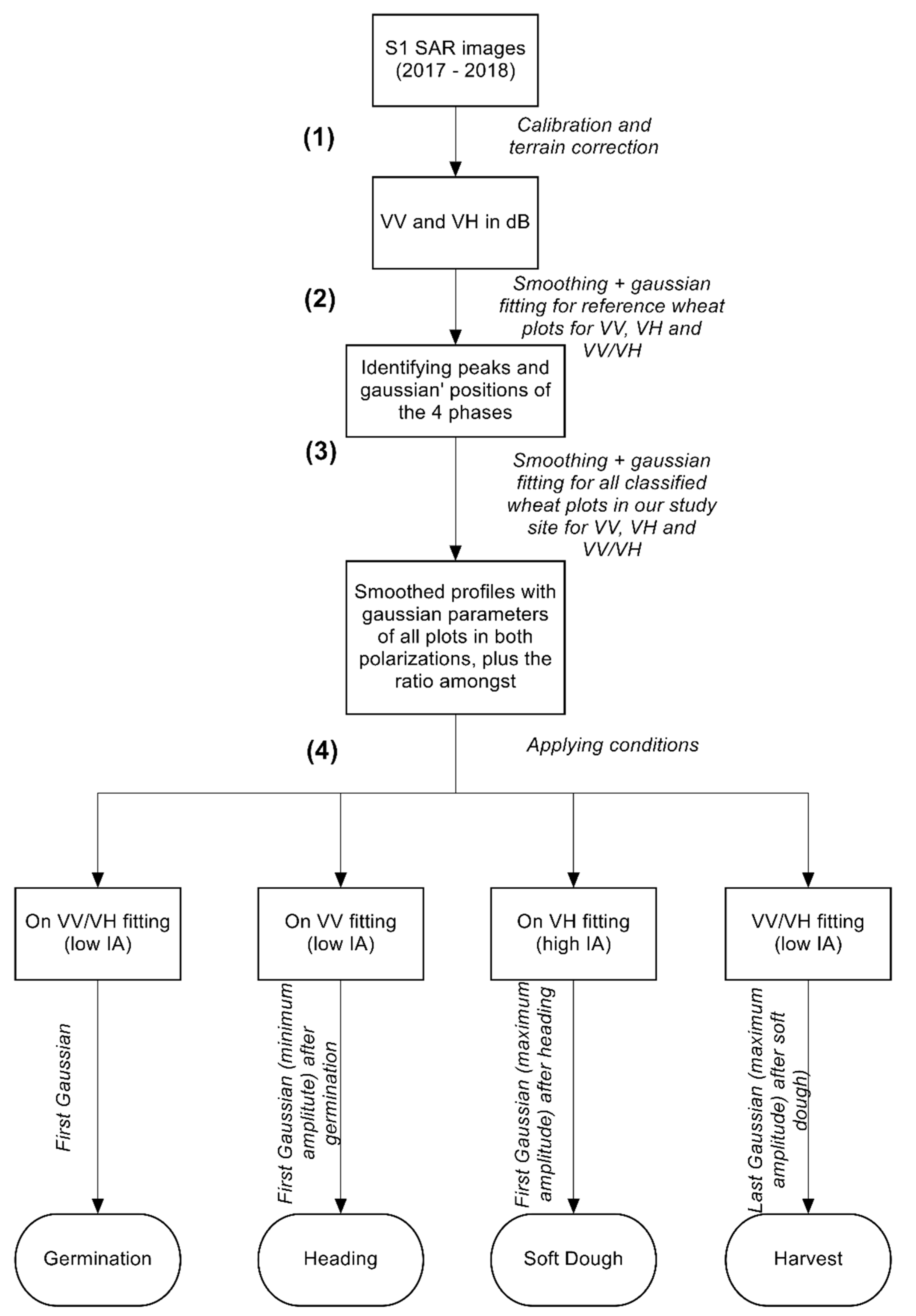
Figure 3.
Winter wheat Normalized Difference Vegetation Index (NDVI) (left y-axis) temporal profiles of both parts of the study site (West (a) and North (b) Bekaa) for the 2017–2018 cropping season versus time expressed as days after sowing (DAS) on the x-axis. On the temporal profiles, the daily precipitation is shown (right y-axis). On each profile, the three main phenological phases are denoted each by a vertical line, in addition to sowing and harvesting dates.
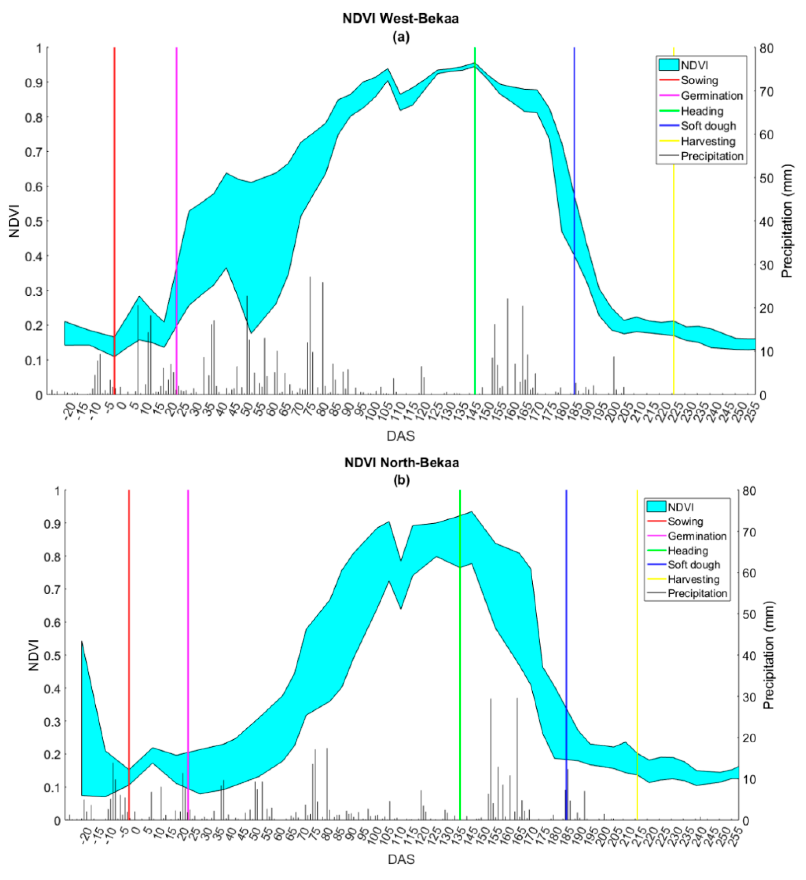
Figure 4.
Winter wheat S1 (left y-axis) temporal profiles, which consist of VV (a,d), VH (b,e) and VV/VH (c,f) at low (32–34°) and high (43–45°) incidence angles of West Bekaa for the 2017–2018 cropping season versus time expressed as days after sowing (DAS) on the x-axis. On the temporal profiles, the daily precipitation is shown (right y-axis). On each profile, each of the three main phenological phases is denoted by a vertical line, in addition to sowing and harvesting dates.
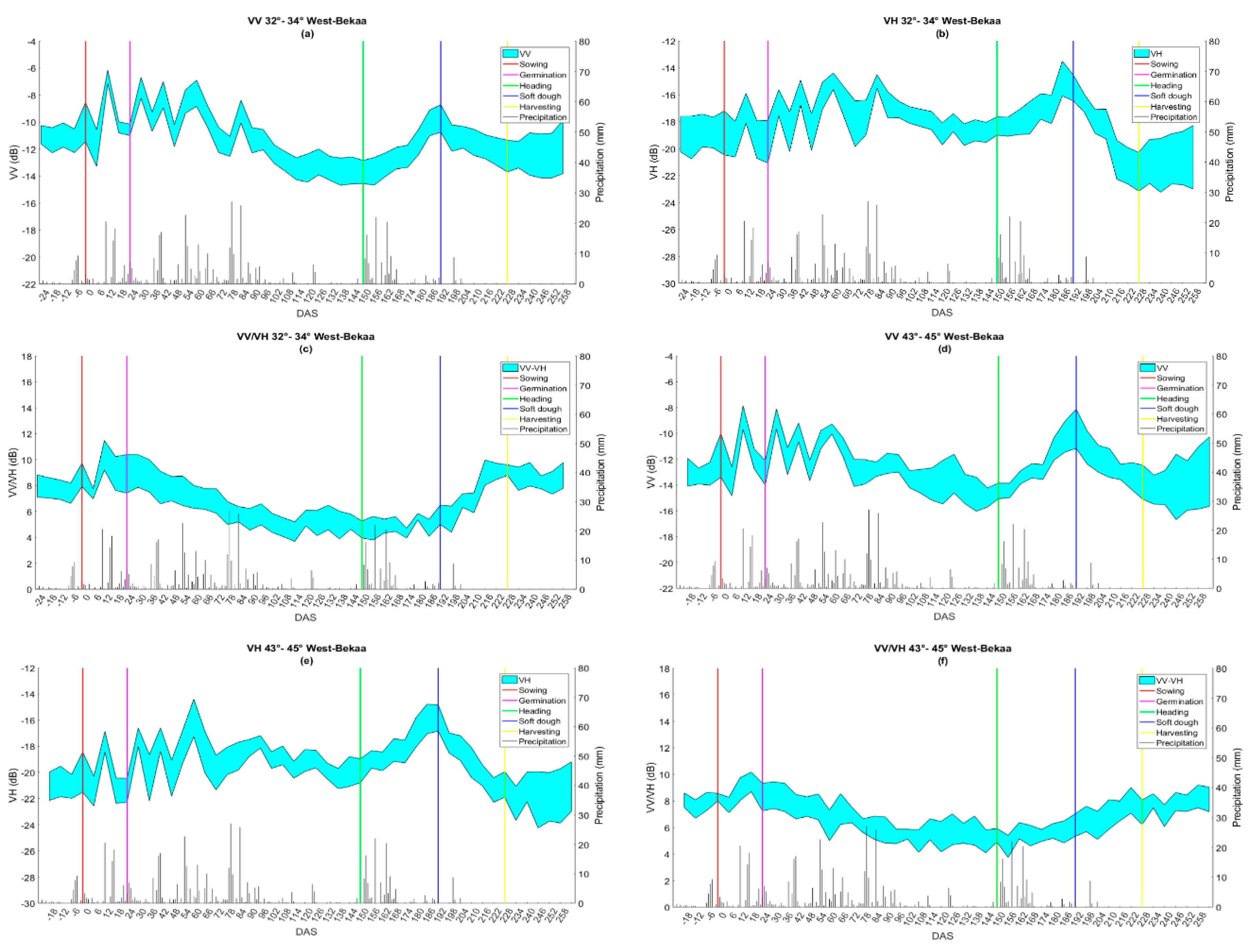
Figure 5.
Air relative humidity (left y-axis) and temperature (right y-axis) versus date (x-axis) for both parts (West and North Bekaa). The data correspond to the period from heading until physiological maturity (April through June).
Figure 5.
Air relative humidity (left y-axis) and temperature (right y-axis) versus date (x-axis) for both parts (West and North Bekaa). The data correspond to the period from heading until physiological maturity (April through June).
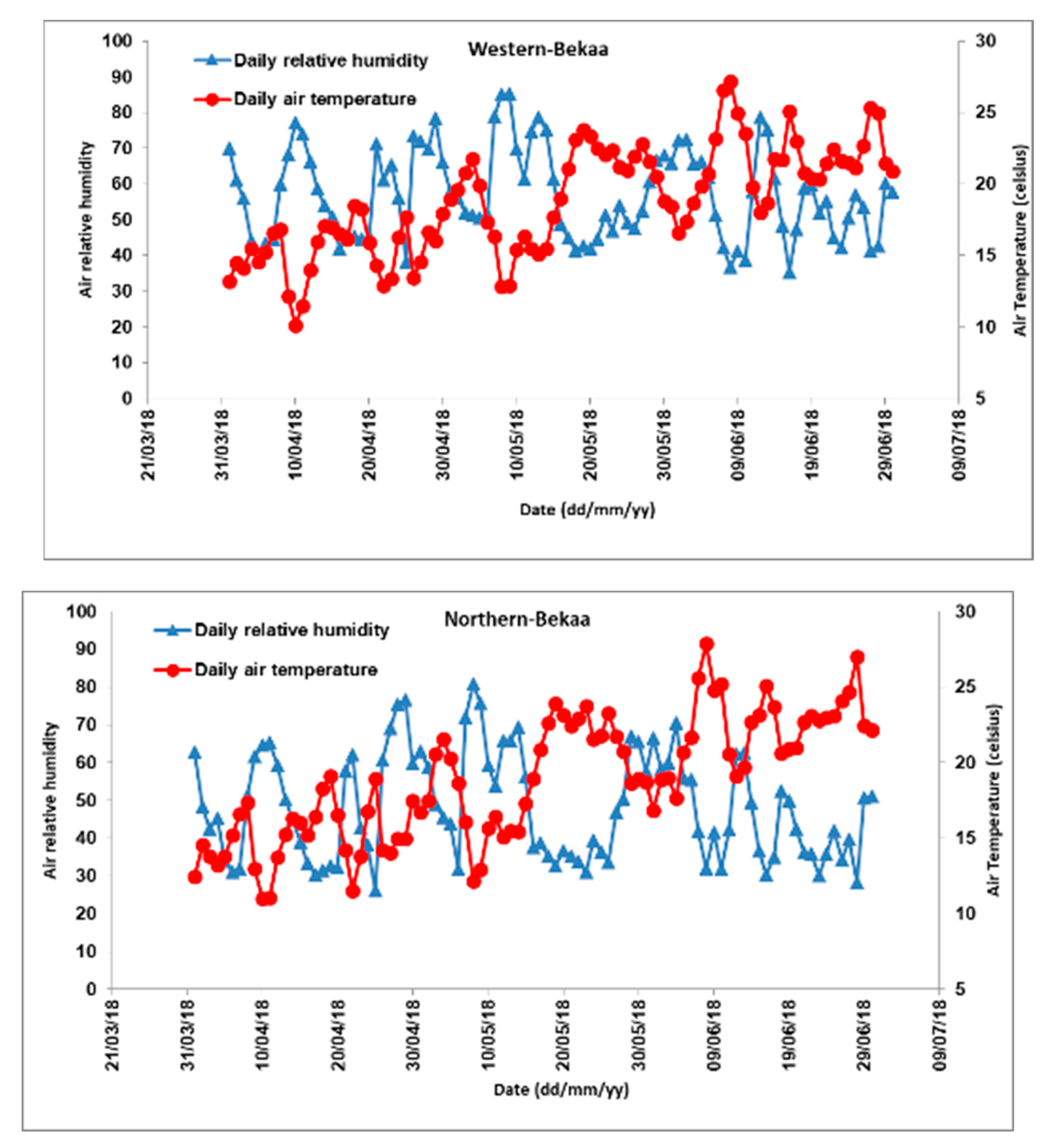
Figure 6.
Gaussian fitting of the S1-VV/VH temporal series of a winter wheat plot at the West Bekaa plain of Lebanon. The incidence angle is 32–34°. The x-axis represents the date and the y-axis refers to the normalized signal. The black arrows indicate the inflection points where germination and harvesting had taken place.
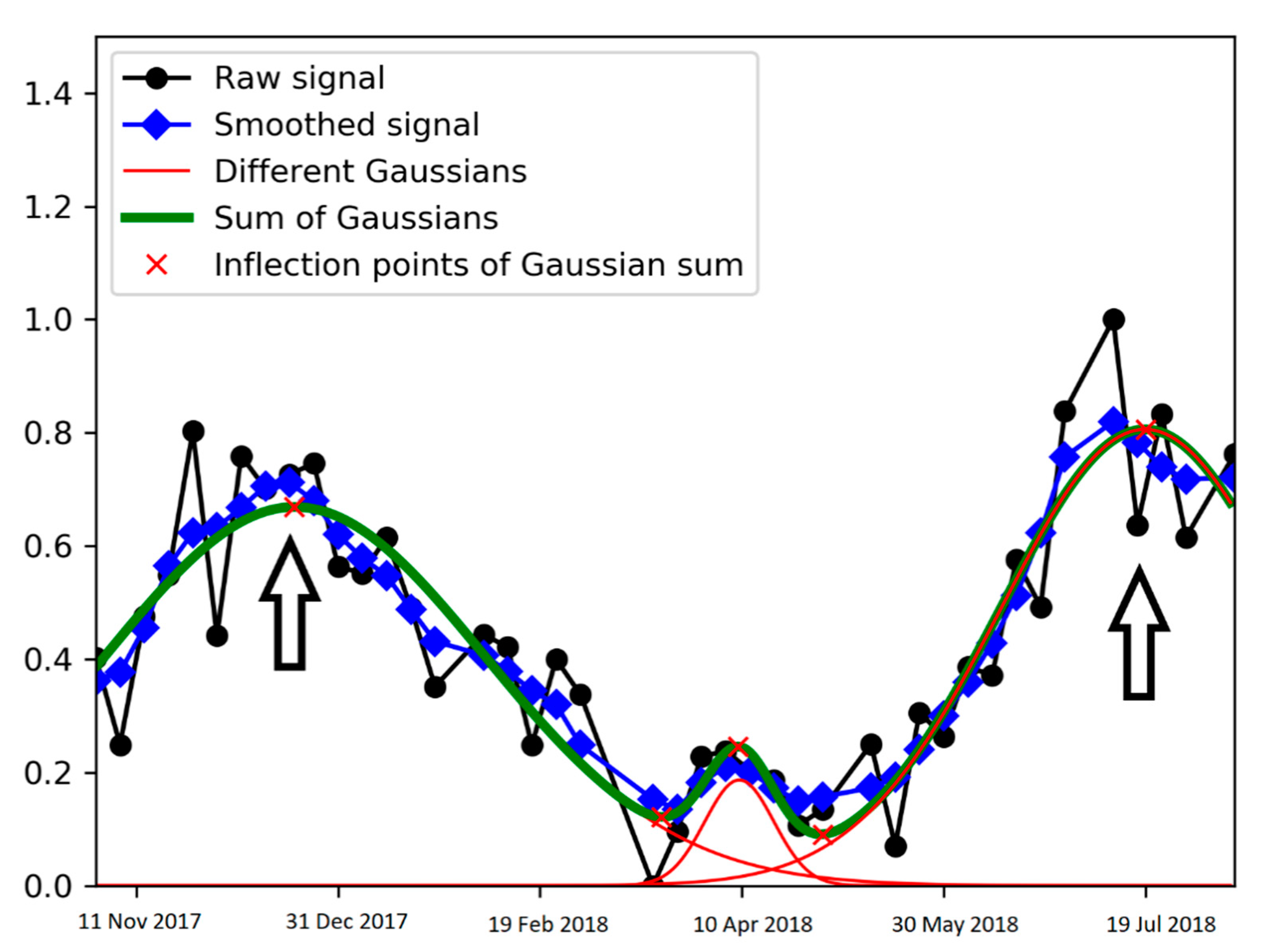
Figure 7.
Gaussian fitting of the S1-VV temporal series of a winter wheat plot at the West Bekaa plain of Lebanon. The incidence angle is 32–34°. The x-axis represents the date and the y-axis refers to the normalized signal. The black arrow indicates the inflection point where heading had taken place.
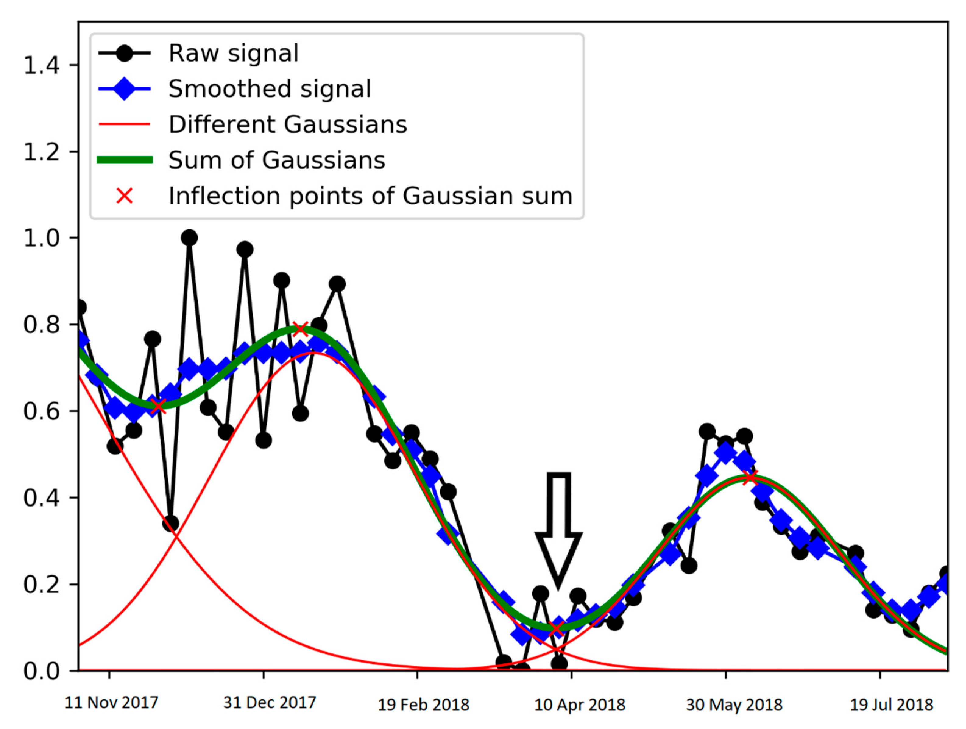
Figure 8.
Gaussian fitting of the S1-VH temporal series of a winter wheat plot at the West Bekaa plain of Lebanon. The incidence angle is 43–45°. The x-axis represents the date and the y-axis refers to the normalized signal. The black arrow indicates the inflection point where soft dough had taken place.
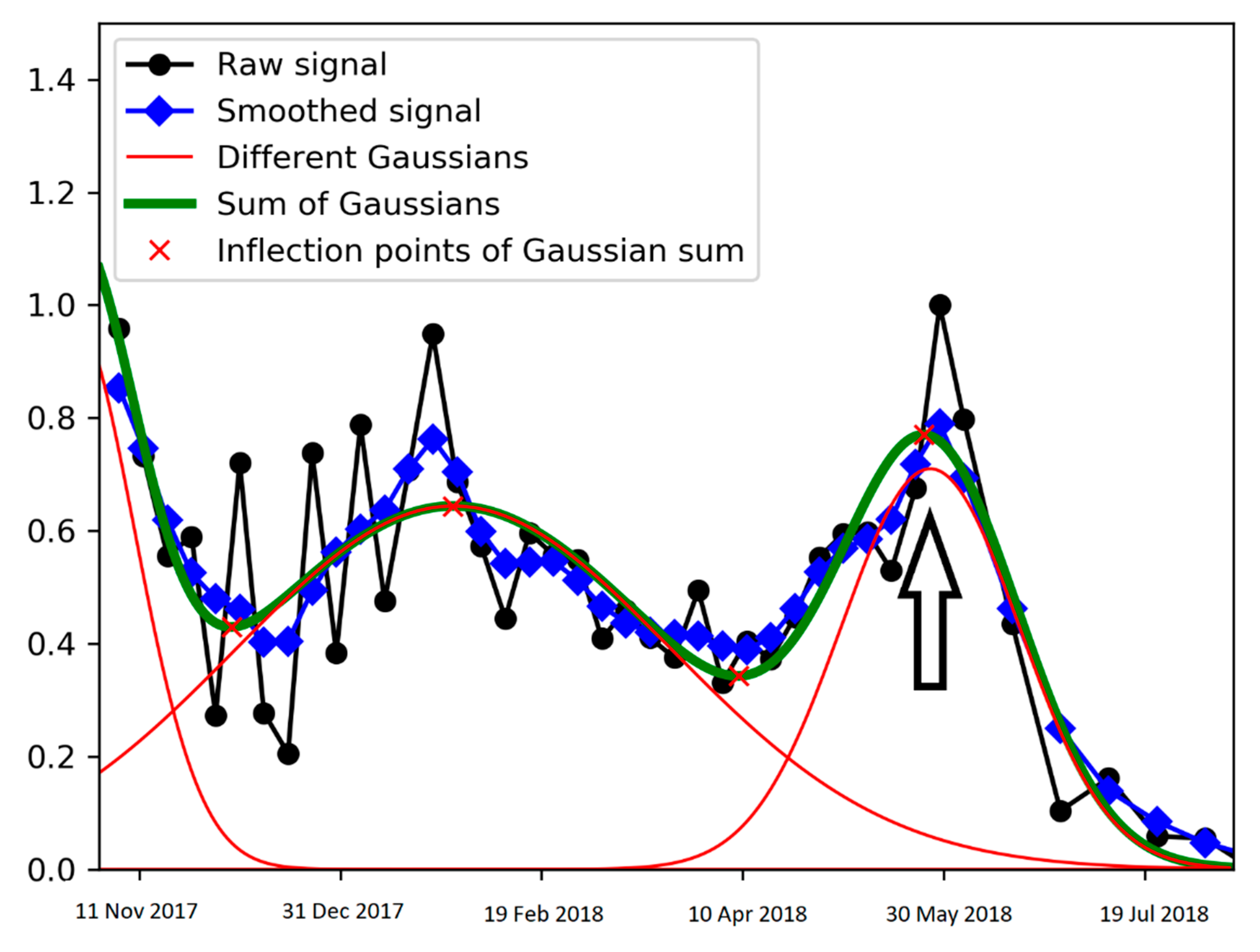
Figure 9.
Maps of the three phenological phases’ dates and the harvesting for West Bekaa (WB) and harvesting for North Bekaa (NB) extracted from S1 Gaussians fitting parameters. For each map, the color bar reflects the time of achieving each phase by each winter wheat plot.
Figure 9.
Maps of the three phenological phases’ dates and the harvesting for West Bekaa (WB) and harvesting for North Bekaa (NB) extracted from S1 Gaussians fitting parameters. For each map, the color bar reflects the time of achieving each phase by each winter wheat plot.


Figure 10.
The estimated versus the observed dates recorded in situ for the three phenological phases and the harvesting. The phases correspond to germination (a), heading (b), and soft dough (c) for West Bekaa, in addition to the harvesting event for both West (d) and North (e) Bekaa. The Root Mean Square Error (RMSE) and the difference between the estimated and the observed dates (bias) are displayed on each of the graphs. The blue dots represent the dates and the red line corresponds to 1:1.
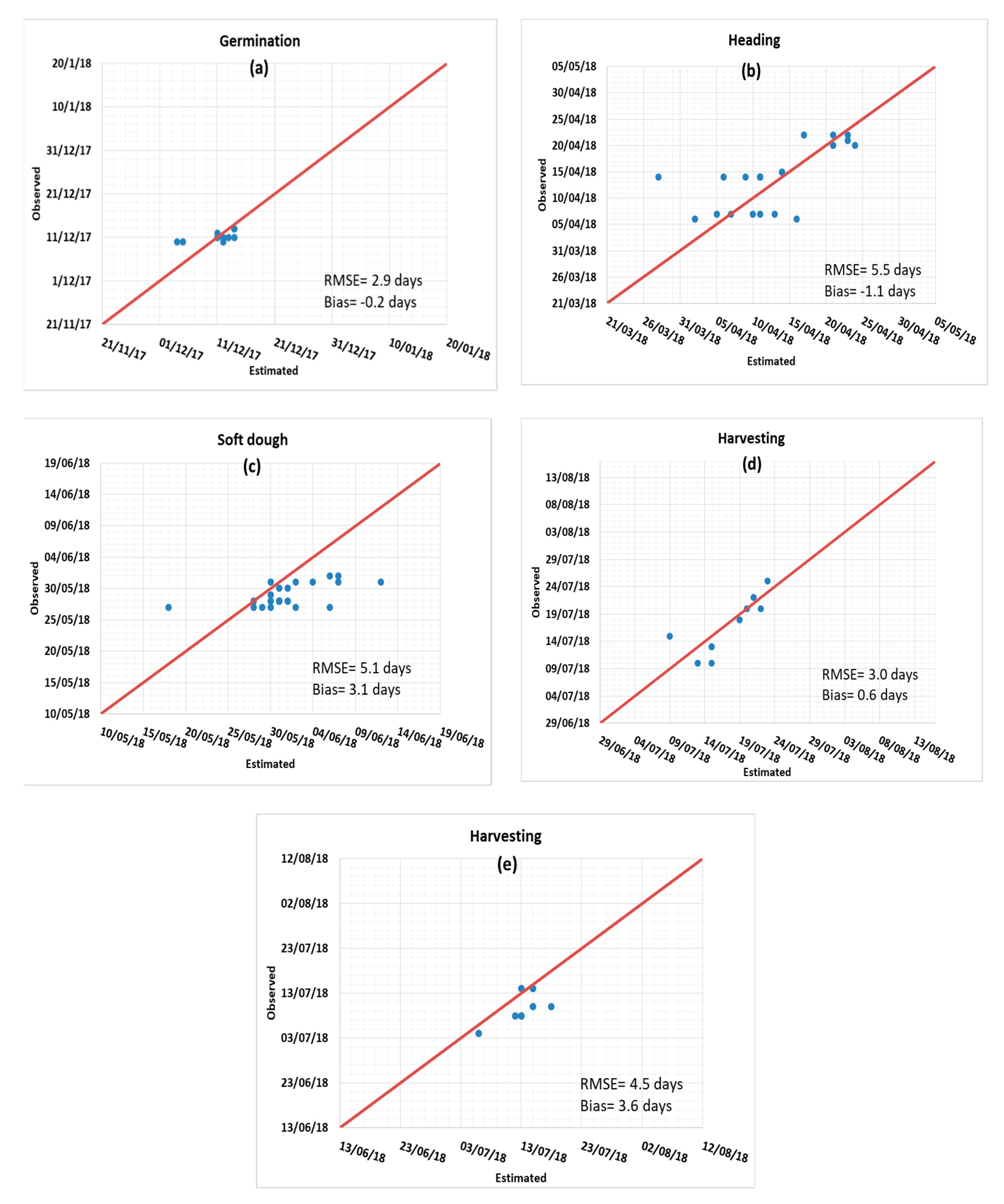
Figure 11.
Gaussian fitting of a winter wheat plot at 32–34° (a), and 43–45° (b), in the VH polarization. The black arrow indicates the soft dough phase.
Figure 11.
Gaussian fitting of a winter wheat plot at 32–34° (a), and 43–45° (b), in the VH polarization. The black arrow indicates the soft dough phase.
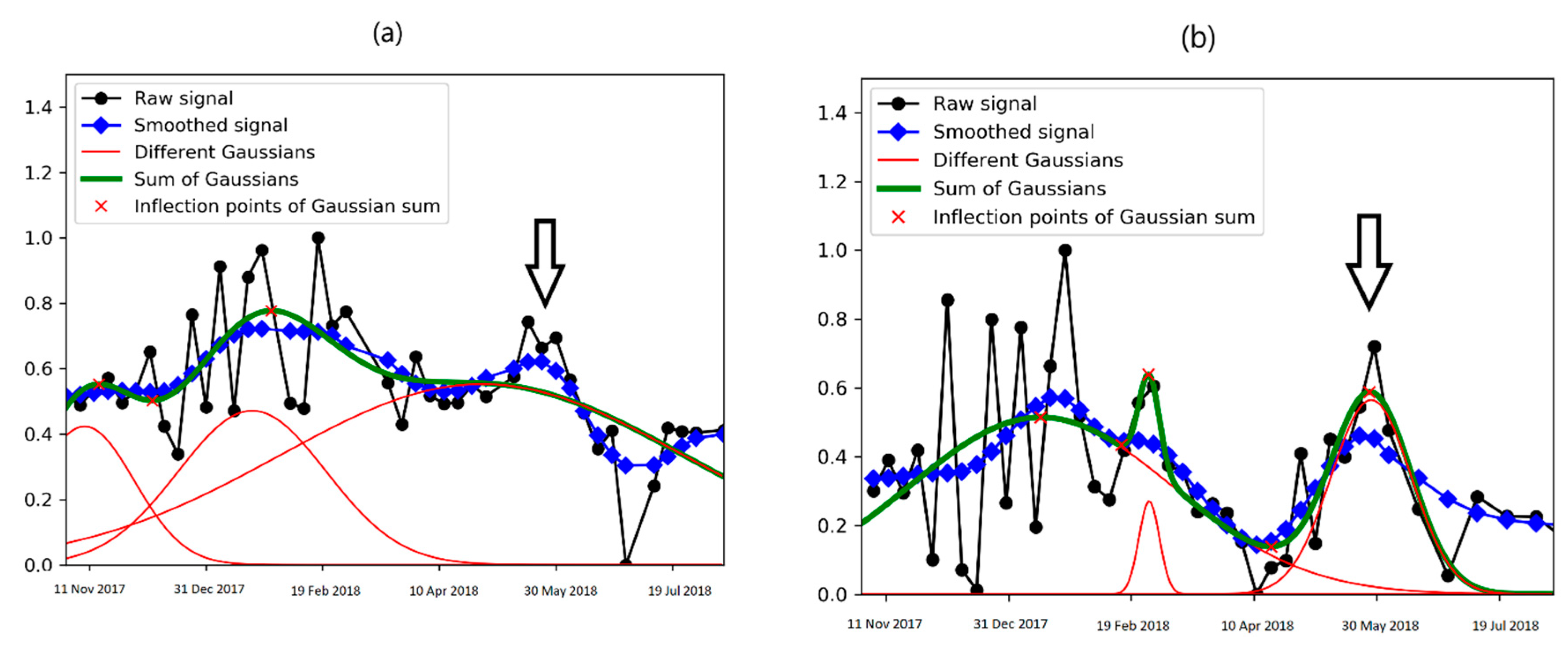

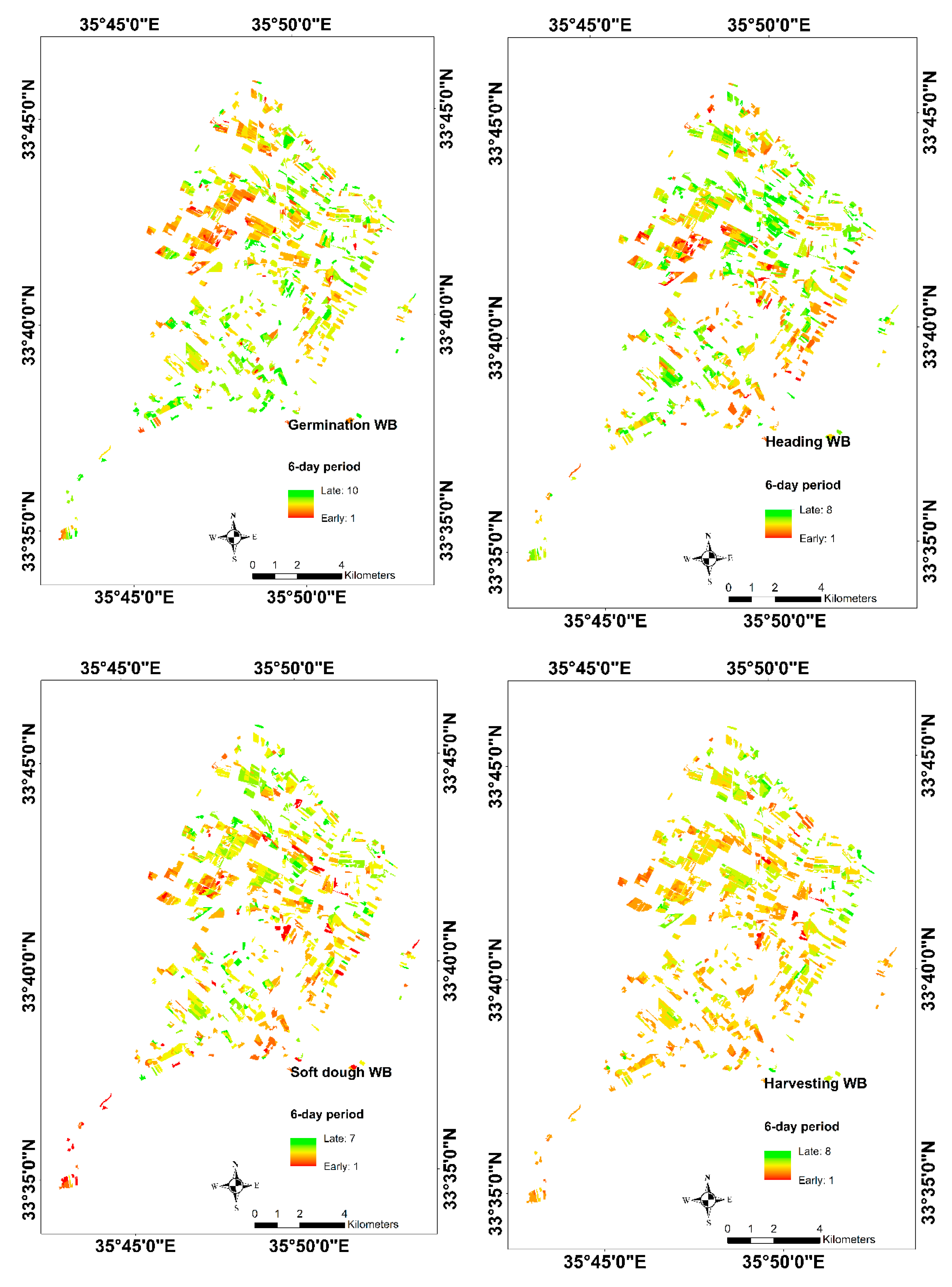
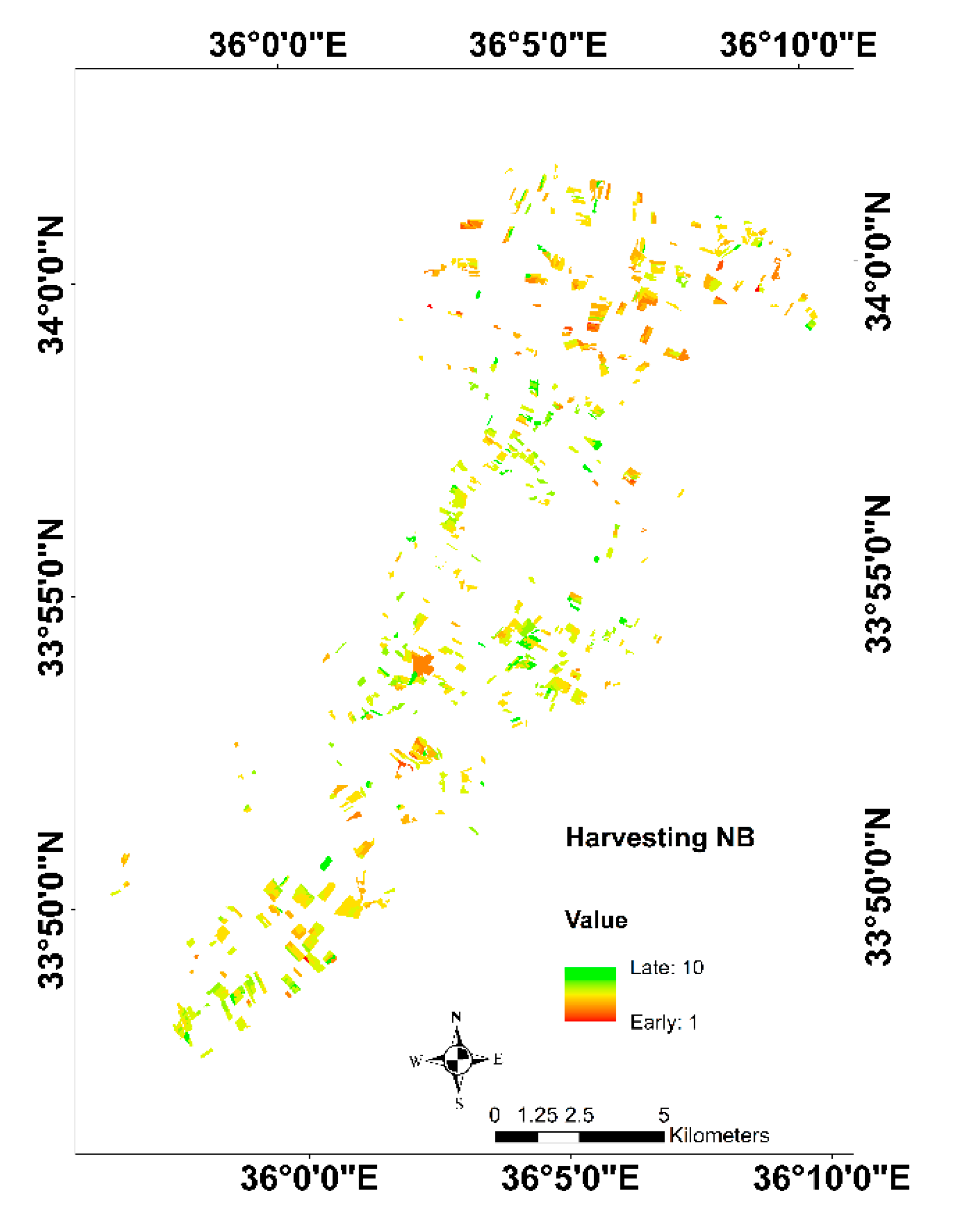
Table 1.
Dates of the three phenological phases plus the harvesting of the reference plots within the West Bekaa (WB) plain as well as for harvesting for North Bekaa (NB) plain. “—” signifies the unavailable date.
Table 1.
Dates of the three phenological phases plus the harvesting of the reference plots within the West Bekaa (WB) plain as well as for harvesting for North Bekaa (NB) plain. “—” signifies the unavailable date.
| Plot ID | Germination (Day Month Year) | Heading (Day Month Year) | Soft Dough (Day Month Year) | Harvesting (Day Month Year) |
|---|---|---|---|---|
| 1 (WB) | — | 14 April 2018 | 27 May 2018 | — |
| 2 (WB) | — | 14 April 2018 | 01 June 2018 | — |
| 3 (WB) | 10 December 2017 | 22 April 2018 | 29 May 2018 | 13 July 2018 |
| 4 (WB) | 10 December 2017 | 07 April 2018 | 01 June 2018 | 13 July 2018 |
| 5 (WB) | 11 December 2017 | 22 April 2018 | 28 May 2018 | 20 July 2018 |
| 6 (WB) | — | 07 April 2018 | 31 May 2018 | — |
| 7 (WB) | 12 December 2017 | 07 April 2018 | 27 May 2018 | — |
| 8 (WB) | 11 December 2017 | 22 April 2018 | 27 May 2018 | 22 July 2018 |
| 9 (WB) | 13 December 2017 | 21 April 2018 | 30 May 2018 | 25 July 2018 |
| 10 (WB) | — | 07 April 2018 | 27 May 2018 | — |
| 11 (WB) | — | 07 April 2018 | 27 May 2018 | 10 July 2018 |
| 12 (WB) | — | 14 April 2018 | 27 May 2018 | — |
| 13 (WB) | — | 06 April 2018 | 31 May 2018 | — |
| 14 (WB) | — | 15 April 2018 | 31 May 2018 | — |
| 15 (WB) | — | 15 April 2018 | 28 May 2018 | — |
| 16 (WB) | — | 14 April 2018 | 31 May 2018 | — |
| 17 (WB) | 11 December 2017 | 14 April 2018 | 28 May 2018 | 20 July 2018 |
| 18 (WB) | 10 December 2017 | 14 April 2018 | 31 May 2018 | 10 July 2018 |
| 19 (WB) | — | 06 April 2018 | 28 May 2018 | — |
| 20 (WB) | 13 December 2017 | 20 April 2018 | 30 May 2018 | 15 July 2018 |
| 21 (WB) | 11 December 2017 | 20 April 2018 | 28 May 2018 | 18 July 2018 |
| 1 (NB) | — | — | — | 10 July 2018 |
| 2 (NB) | — | — | — | 10 July 2018 |
| 3 (NB) | — | — | — | 04 July 2018 |
| 4 (NB) | — | — | — | 14 July 2018 |
| 5 (NB) | — | — | — | 14 July 2018 |
| 6 (NB) | — | — | — | 08 July 2018 |
| 7 (NB) | — | — | — | 08 July 2018 |
| 8 (NB) | — | — | — | 08 July 2018 |
Table 2.
Means ± standard deviations of NDVI and SAR backscatter (σ°) in VV and VH polarizations in addition to the ratio VV/VH, at low (32–34°) and high (43–45°) incidence angles.
Table 2.
Means ± standard deviations of NDVI and SAR backscatter (σ°) in VV and VH polarizations in addition to the ratio VV/VH, at low (32–34°) and high (43–45°) incidence angles.
| Germination | Heading | Soft dough | Harvesting | |
|---|---|---|---|---|
| NDVI | 0.28 ± 0.07 | 0.94 ± 0.05 | 0.48 ± 0.08 | 0.19 ± 0.01 |
| VV 32–34° | −10.58 ± −0.43 | −13.8 ± −0.75 | −9.74 ± −1.02 | −12.53 ± −1.18 |
| VH 32–34° | −19.48 ± −1.6 | −18.39 ± −0.67 | −16.0 ± −0.96 | −21.71 ± −1.44 |
| VV/VH 32–34° | 8.9 ± 1.5 | 4.64 ± 0.66 | 5.75 ± 0.75 | 9.2 ± 0.4 |
| VV 43–45° | −8.85 ± −0.75 | −14.42 ± −0.57 | −11.18 ± −1.36 | −14.35 ± −1.12 |
| VH 43–45° | −21.35 ± −0.91 | −19.87 ± −0.92 | −15.9 ± −1.09 | −22.38 ± −1.3 |
| VV/VH 43–45° | 8.43 ± 0.99 | 4.58 ± 0.83 | 6.65 ± 0.95 | 7.01 ± 0.51 |
Table 3.
The best S1 configuration (polarization and incidence angle) for phenological phases (i.e., germination, heading and soft dough) and harvesting mapping in addition to the way of determination for each.
Table 3.
The best S1 configuration (polarization and incidence angle) for phenological phases (i.e., germination, heading and soft dough) and harvesting mapping in addition to the way of determination for each.
| Phase | Polarization | Incidence Angle | Way of Determination |
|---|---|---|---|
| Germination | VV/VH | 32°–34° | First peak in the sum of Gaussians fitting (positive derivative) |
| Heading | VV | 32°–34° | First minimum after germination in the sum of Gaussians fitting (identification starts after germination date) |
| Soft dough | VH | 43°–45° | First maximum after heading in the sum of Gaussians fitting (identification starts after the heading date) |
| Harvesting | VV/VH | 32°–34° | Last maximum after soft dough in the sum of Gaussians fitting (identification starts after soft dough date) |
Table 4.
Winter wheat plots’ percentages for each mapped phenological phase of West Bekaa plus the harvesting of West (WB) and North (NB) Bekaa, in each 6-day period.
Table 4.
Winter wheat plots’ percentages for each mapped phenological phase of West Bekaa plus the harvesting of West (WB) and North (NB) Bekaa, in each 6-day period.
| Event | Corresponding Period (Day Month Year) | Percentage of Plots (%) |
|---|---|---|
| Germination (WB) | 21 November 2017–27 November 2017 | 2.0 |
| 27 November 2017–03 December 2017 | 4.7 | |
| 03 December 2017–09 December 2017 | 11.0 | |
| 09 December 2017–15 December 2017 | 14.8 | |
| 15 December 2017–21 December 2017 | 18.3 | |
| 21 December 2017–27 December 2017 | 18.0 | |
| 27 December 2017–02 January 2018 | 17.2 | |
| 02 January 2018–08 January 2018 | 8.0 | |
| 08 January 2018–14 January 2018 | 3.5 | |
| 14 January 2018–20 January 2018 | 2.5 | |
| Heading (WB) | 21 March 2018–27 March 2018 | 4.2 |
| 27 March 2018–02 April 2018 | 10.2 | |
| 02 April 2018–08 April 2018 | 16.0 | |
| 08 April 2018–14 April 2018 | 22.0 | |
| 14 April 2018–20 April 2018 | 19.1 | |
| 20 April 2018–26 April 2018 | 15.8 | |
| 26 May 2018–02 May 2018 | 10.9 | |
| 02 May 2018–04 May 2018 | 1.8 | |
| Soft dough (WB) | 10 May 2018–16 May 2018 | 6.3 |
| 16 May 2018–22 May 2018 | 13.3 | |
| 22 May 2018–28 May 2018 | 26.2 | |
| 28 May 2018–03 June 2018 | 32.0 | |
| 03 June 2018–09 June 2018 | 15.8 | |
| 09 June 2018–15 June 2018 | 5.4 | |
| 15 June 2018–18 June 2018 | 1.0 | |
| Harvesting (WB) | 14 June 2018–20 June 2018 | 0 |
| 20 June 2018–26 June 2018 | 0 | |
| 26 June 2018–02 July 2018 | 0.3 | |
| 02 July 2018–08 July 2018 | 2.5 | |
| 08 July 2018–14 July 2018 | 12.2 | |
| 14 July 2018–20 July 2018 | 27.5 | |
| 20 July 2018–26 July 2018 | 40.4 | |
| 26 July 2018–01 August 2018 | 12.1 | |
| 01 August 2018–07 August 2018 | 3.8 | |
| 07 August 2018–13 August 2018 | 0.9 | |
| 13 August 2018–16 August 2018 | 0.3 | |
| Harvesting (NB) | 14 June 2018–20 June 2018 | 0.5 |
| 20 June 2018–26 June 2018 | 1.3 | |
| 26 June 2018–02 July 2018 | 5.5 | |
| 02 July 2018–08 July 2018 | 15.6 | |
| 08 July 2018–14 July 2018 | 29.2 | |
| 14 July 2018–20 July 2018 | 28.7 | |
| 20 July 2018–26 July 2018 | 11.2 | |
| 26 July 2018–01 August 2018 | 4.5 | |
| 01 August 2018–07 August 2018 | 2.2 | |
| 07 August 2018–13 August 2018 | 1.3 | |
| 13 August 2018–16 August 2018 | 0 |
Table 5.
The difference between the estimated and observed dates (bias), the RMSE of the estimated phenological date, and the percent (%) of reference plots for which the date of the different phenological phases could be estimated when the time series ended on the date of the phenological phase, 6, 12, and 18 days later.
| No Image | 1 S1 Image | 2 S1 Images | 3 S1 Images | |||||||||
|---|---|---|---|---|---|---|---|---|---|---|---|---|
| Bias | RMSE (Days) | %Ref Plots | Bias | RMSE (Days) | %Ref Plots | Bias | RMSE (Days) | %Ref Plots | Bias | RMSE (Days) | %Ref Plots | |
| Germination | 14.0 | 20.8 | 80 | 12.9 | 19.1 | 80 | 13.5 | 18.6 | 80 | 7.9 | 9.6 | 100 |
| Heading | −17.4 | 19.1 | 76.2 | −13.3 | 15.3 | 81 | −8.6 | 14.7 | 81 | −4.6 | 11.1 | 81 |
| Soft dough | 5.7 | 10.9 | 85.7 | 5.9 | 10.5 | 85.7 | 3.2 | 6.1 | 100 | 3.1 | 6.1 | 100 |
| Harvesting | −10.7 | 11.7 | 60 | −8.7 | 11.3 | 70 | −3.7 | 3.9 | 70 | 1.9 | 3.9 | 70 |
© 2019 by the authors. Licensee MDPI, Basel, Switzerland. This article is an open access article distributed under the terms and conditions of the Creative Commons Attribution (CC BY) license (http://creativecommons.org/licenses/by/4.0/).
Share and Cite
MDPI and ACS Style
Nasrallah, A.; Baghdadi, N.; El Hajj, M.; Darwish, T.; Belhouchette, H.; Faour, G.; Darwich, S.; Mhawej, M. Sentinel-1 Data for Winter Wheat Phenology Monitoring and Mapping. Remote Sens. 2019, 11, 2228. https://doi.org/10.3390/rs11192228
AMA Style
Nasrallah A, Baghdadi N, El Hajj M, Darwish T, Belhouchette H, Faour G, Darwich S, Mhawej M. Sentinel-1 Data for Winter Wheat Phenology Monitoring and Mapping. Remote Sensing. 2019; 11(19):2228. https://doi.org/10.3390/rs11192228
Chicago/Turabian StyleNasrallah, Ali, Nicolas Baghdadi, Mohammad El Hajj, Talal Darwish, Hatem Belhouchette, Ghaleb Faour, Salem Darwich, and Mario Mhawej. 2019. "Sentinel-1 Data for Winter Wheat Phenology Monitoring and Mapping" Remote Sensing 11, no. 19: 2228. https://doi.org/10.3390/rs11192228
Note that from the first issue of 2016, this journal uses article numbers instead of page numbers. See further details here.