Long-Term Changes of Open-Surface Water Bodies in the Yangtze River Basin Based on the Google Earth Engine Cloud Platform


Abstract
:1. Introduction
2. Materials and Methods
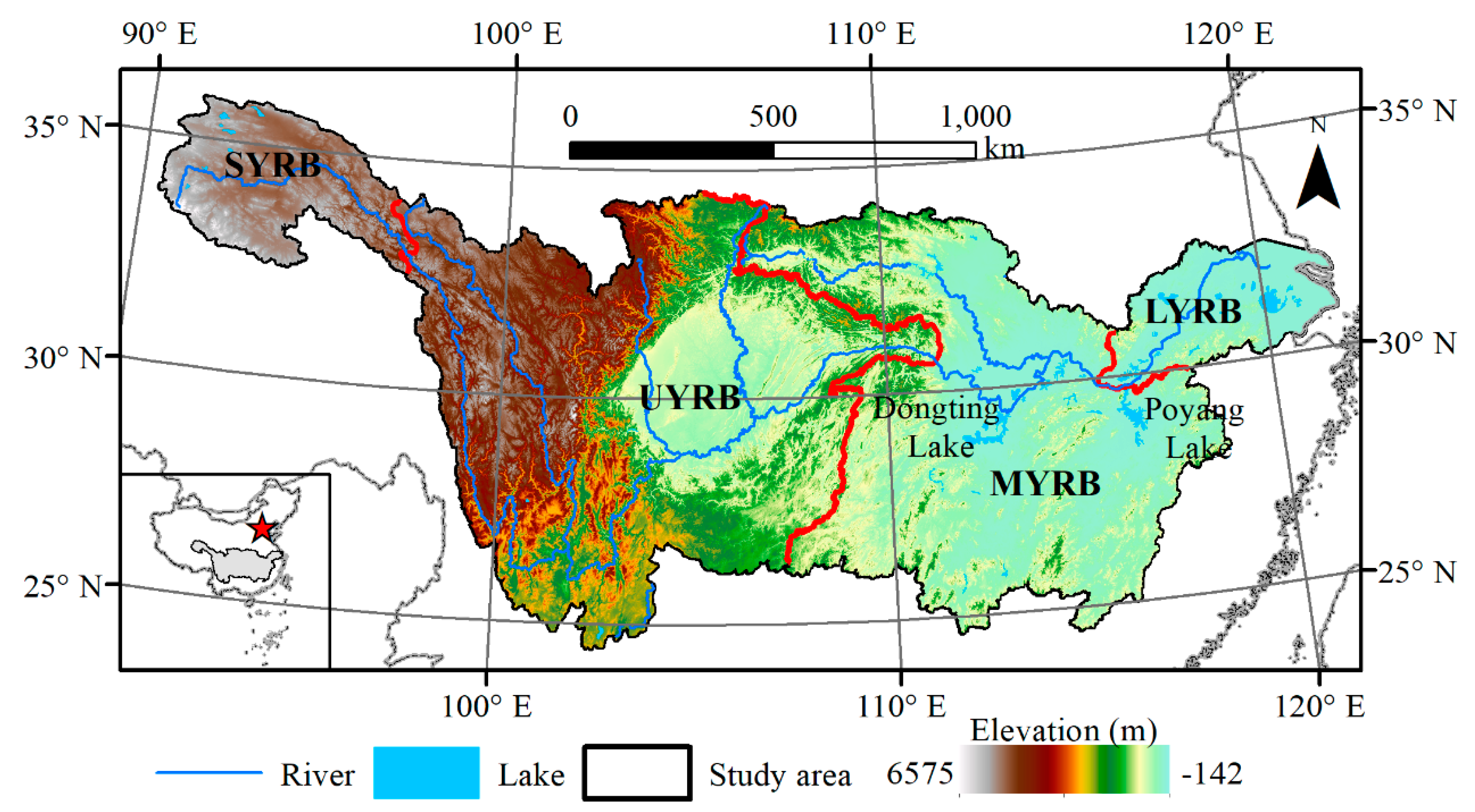
2.1. Study Area
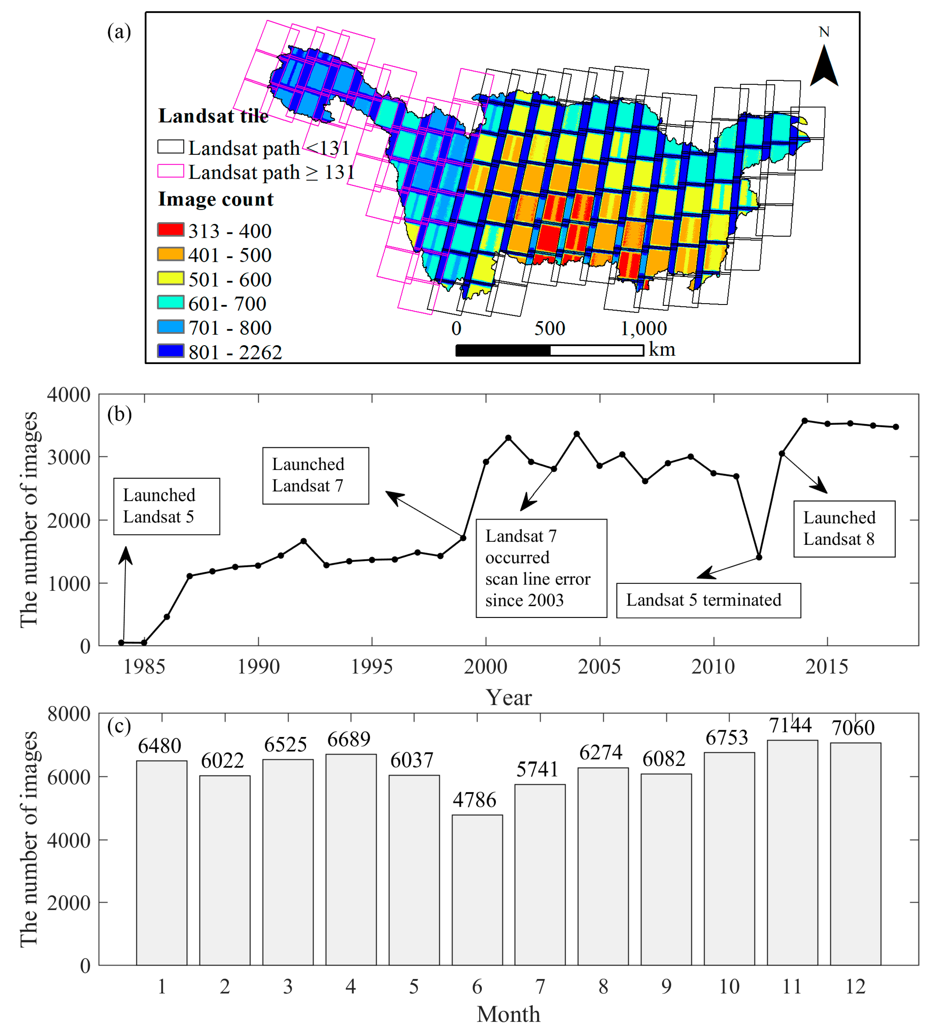
2.2. Data
2.3. Methods
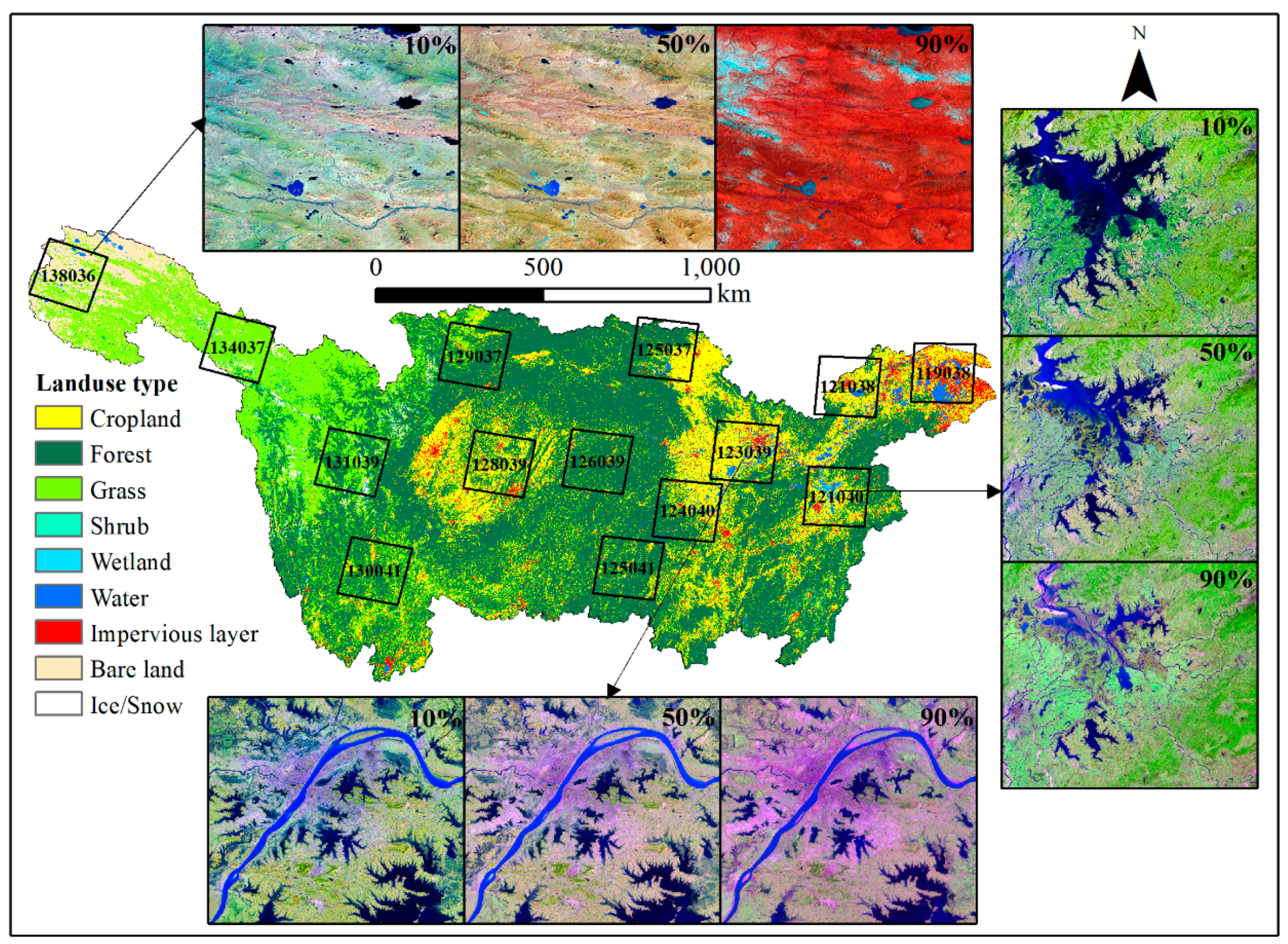
2.3.1. Sample Collection Based on Percentile Composite Images
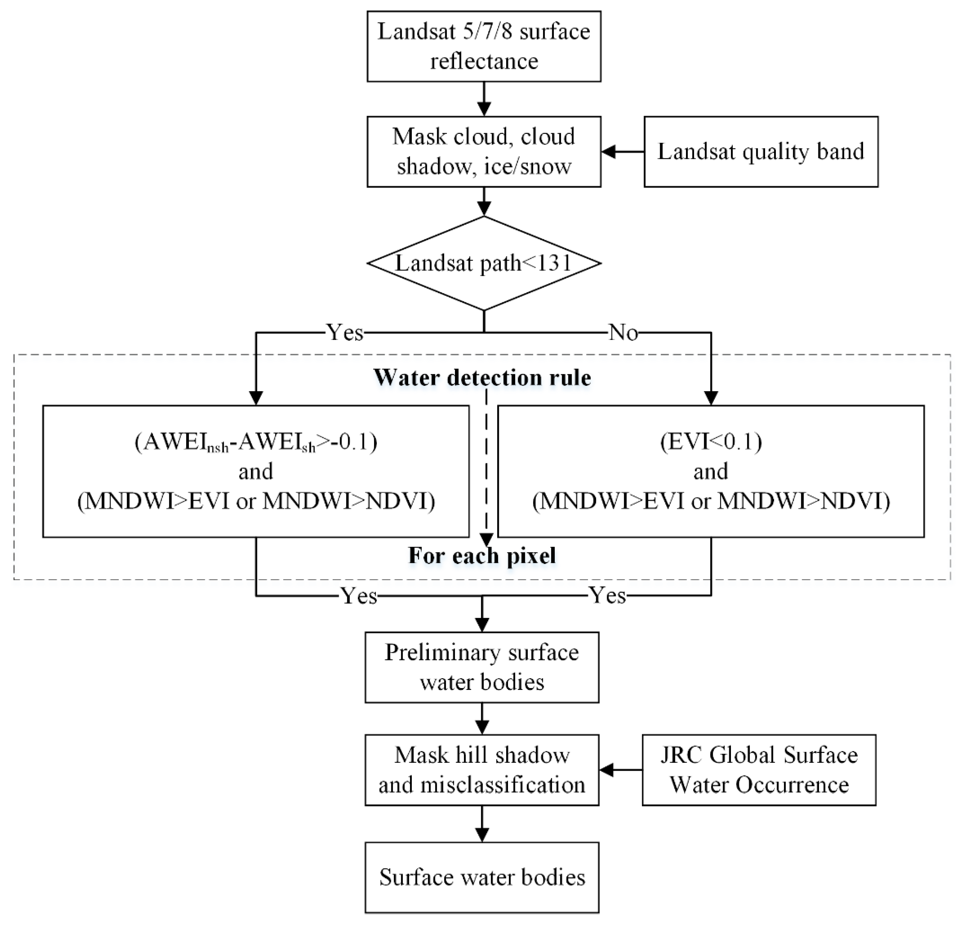
2.3.2. Water Extraction Based on Water Detection Rule
2.3.3. Accuracy Assessment Based on Sentinel-2 Images
2.3.4. Change Analysis of an Open-Surface Water Body
3. Results
3.1. Accuracy of Extracted Open-Surface Water Bodies in the YRB
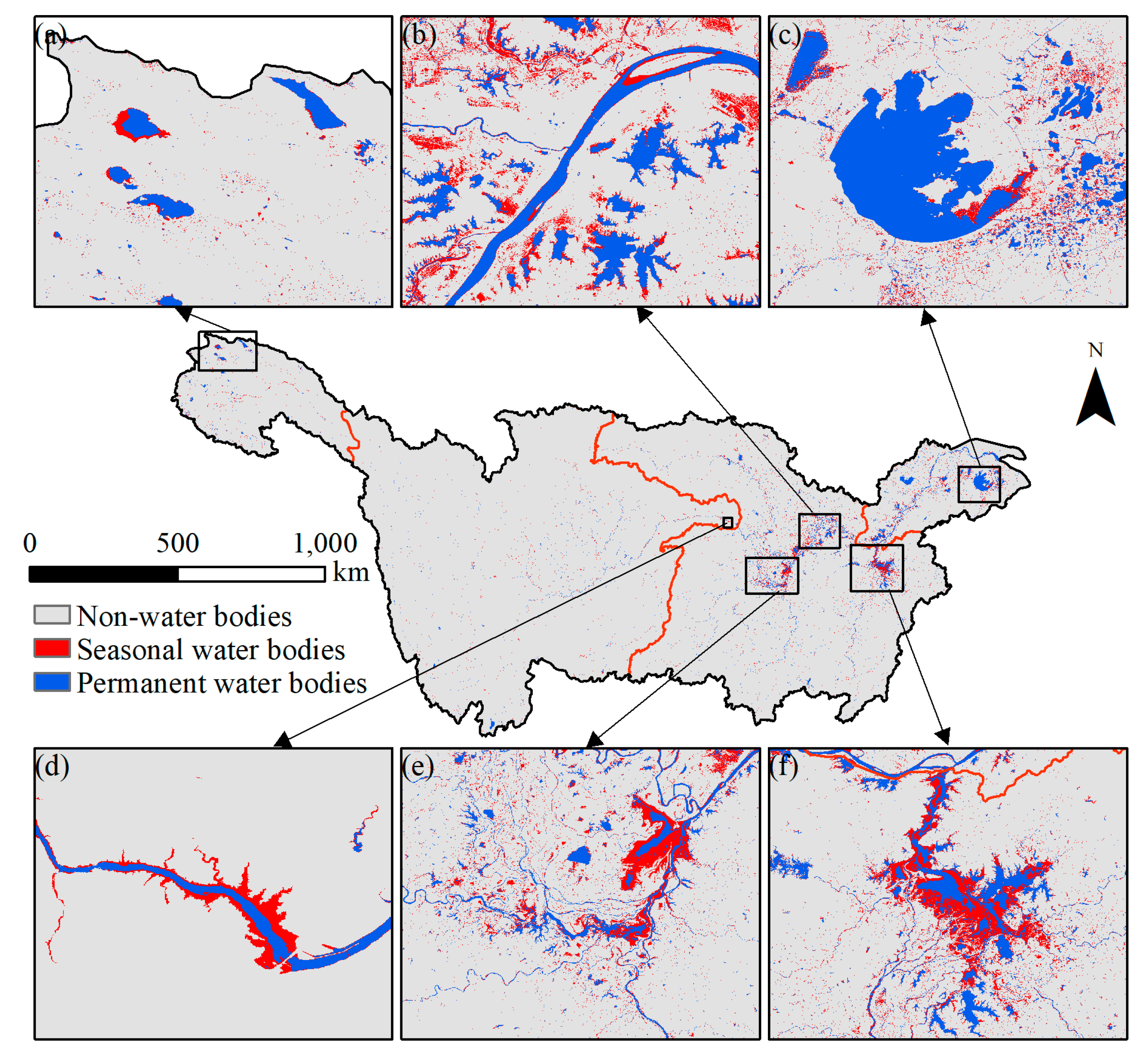
3.2. Spatial Distribution of the Open-Surface Water Bodies in the YRB
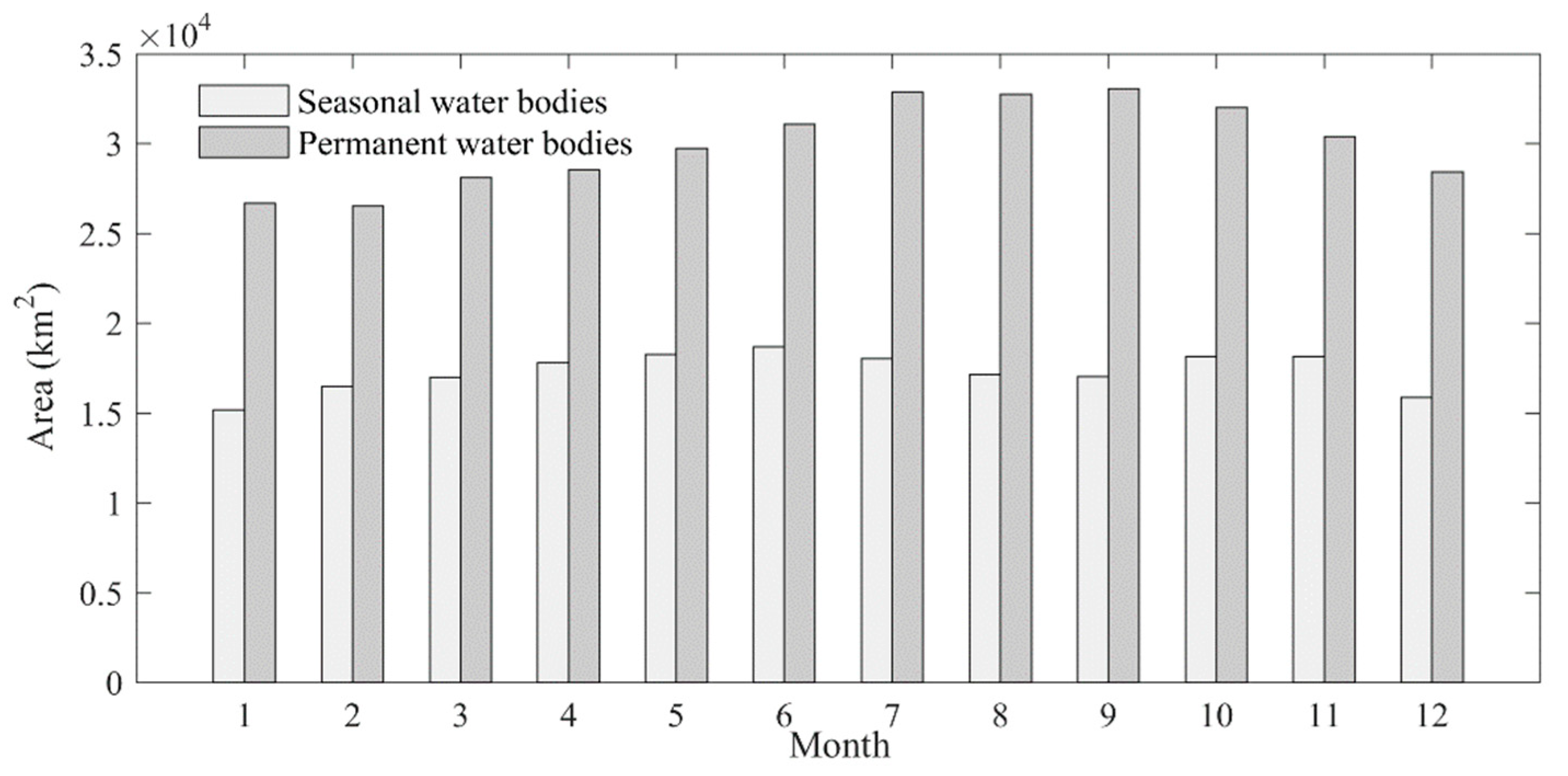
3.3. Monthly Variations of the Surface Water Bodies in the YRB
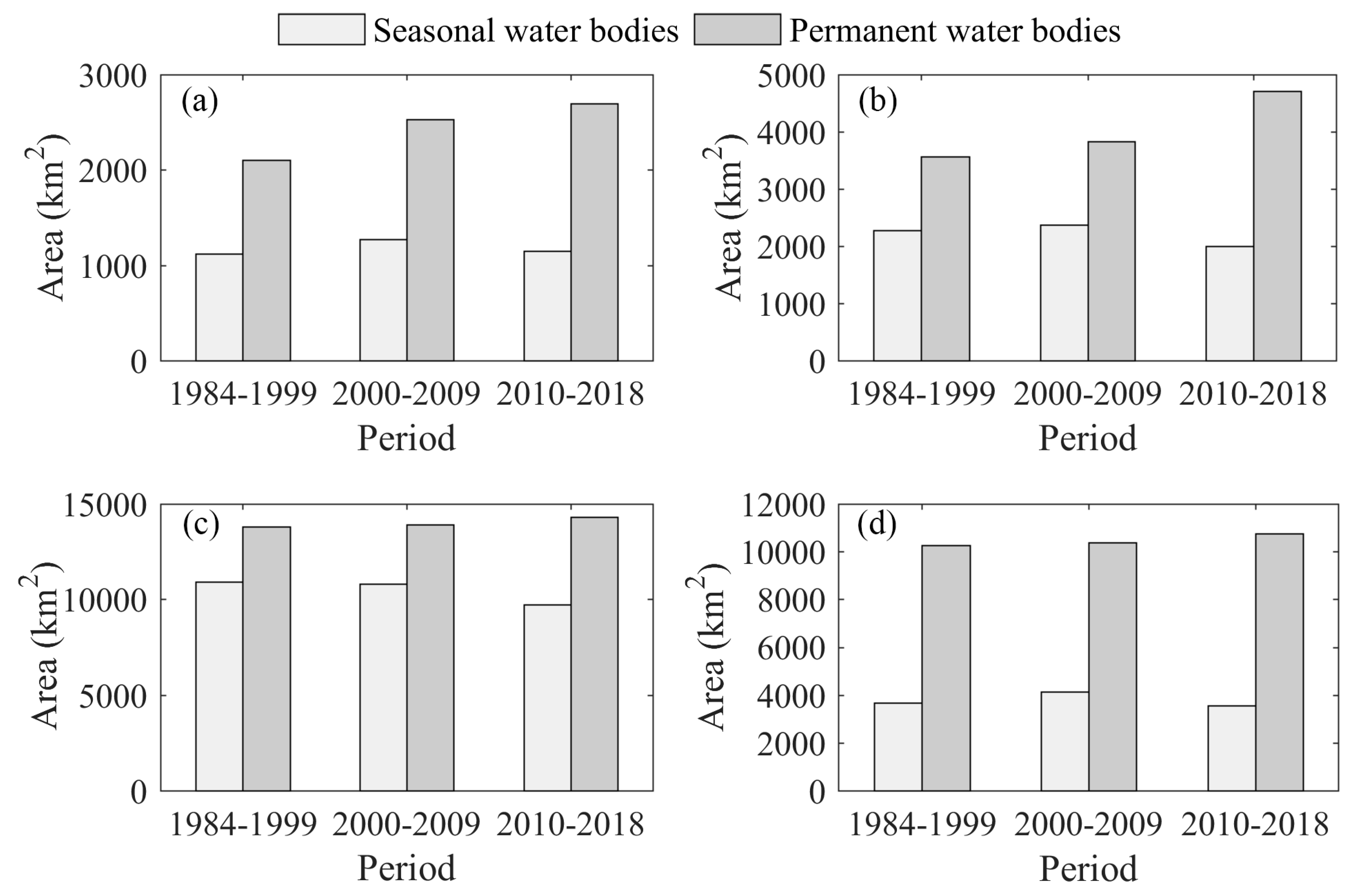
3.4. Temporal Trends of the Open-Surface Water Bodies in the YRB
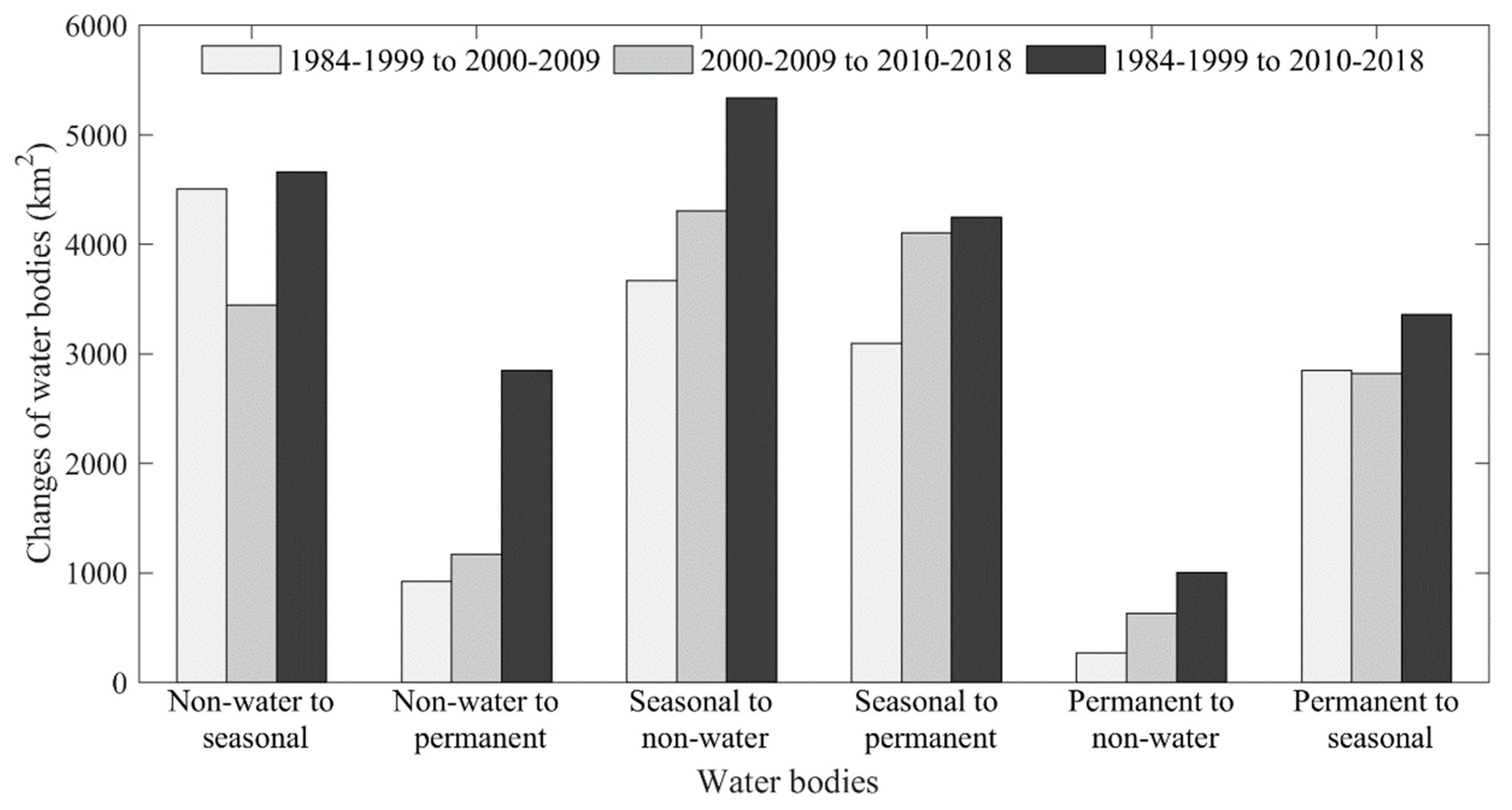
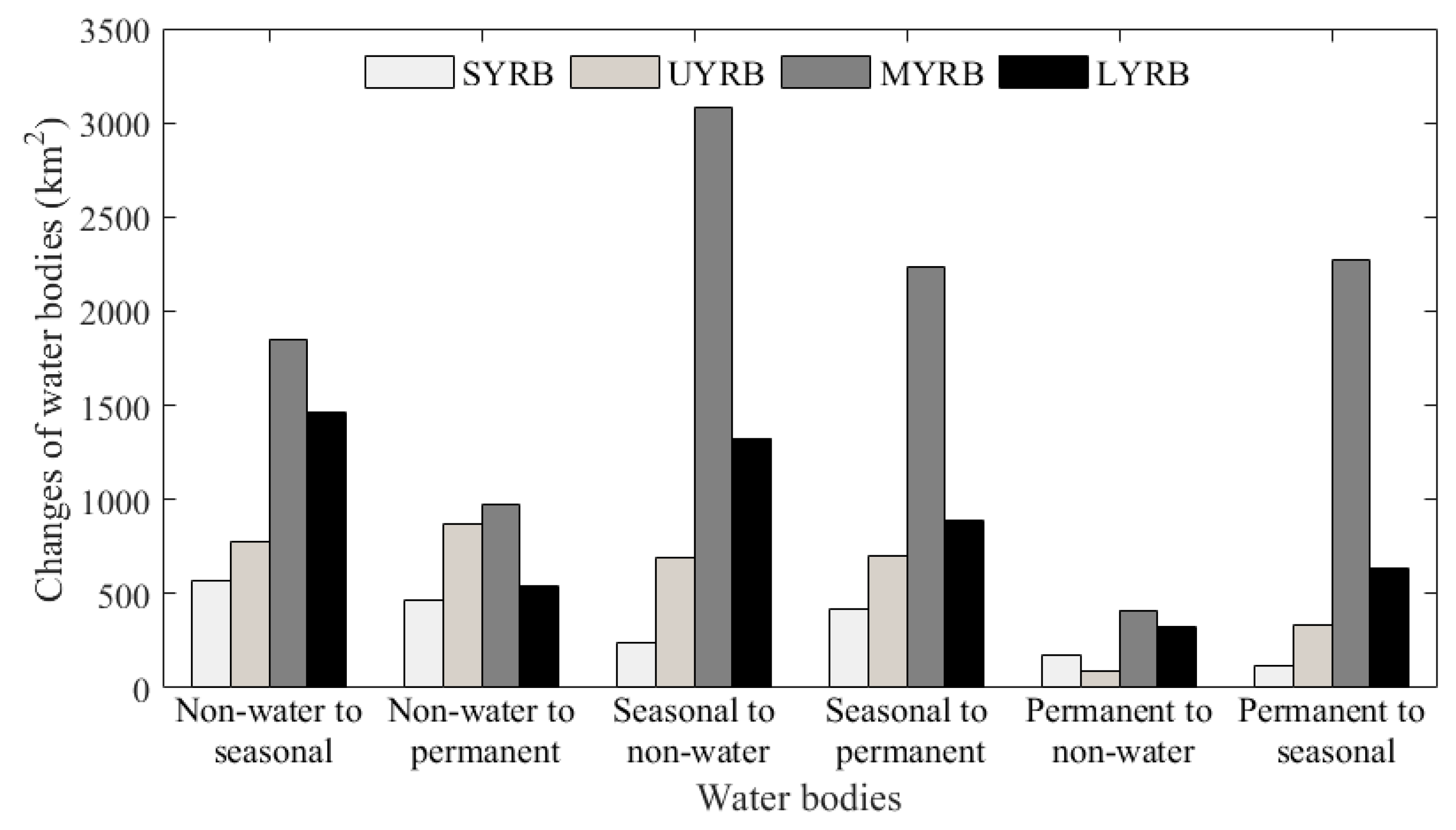
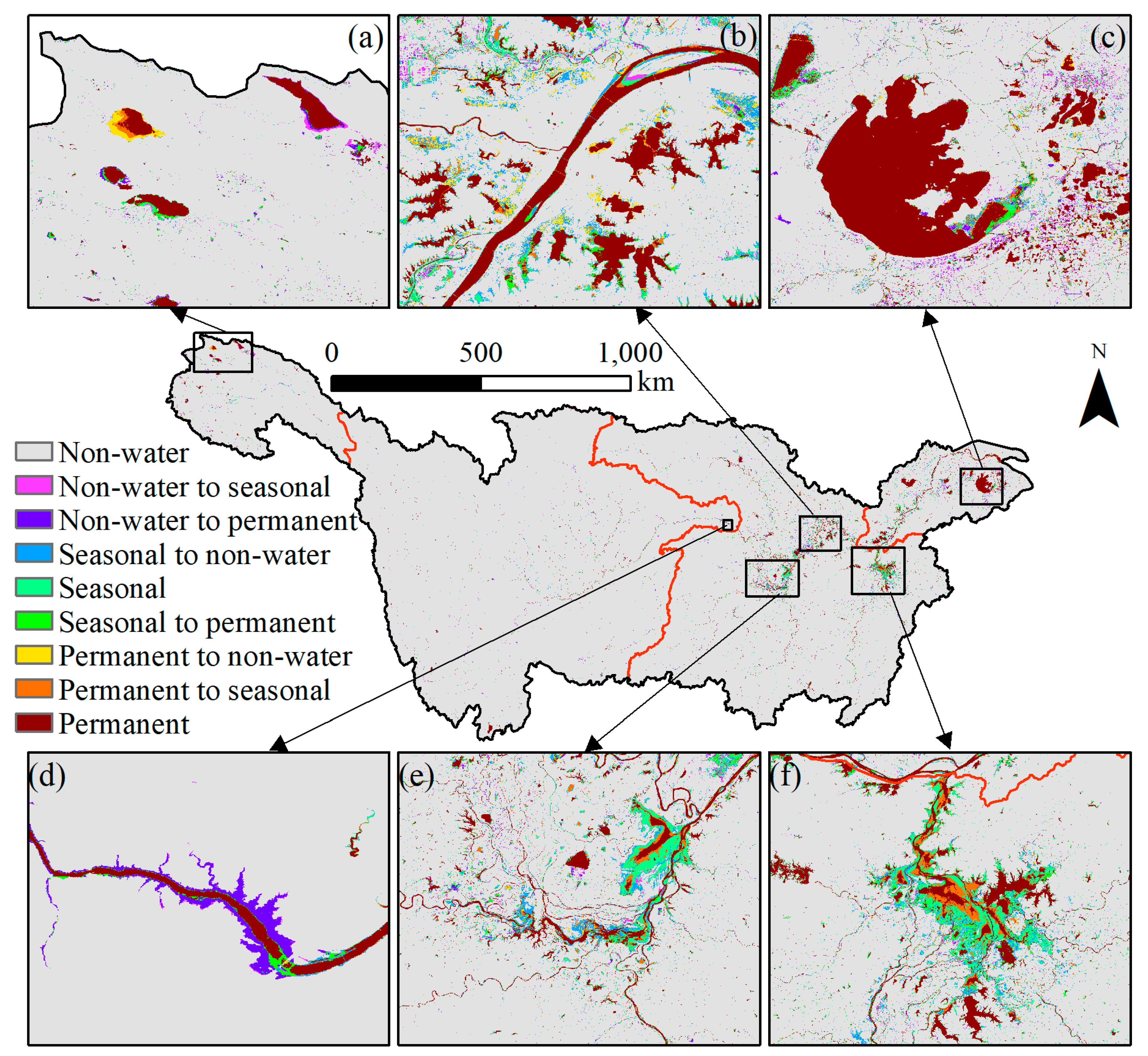
3.5. Conversions of Open-Surface Water Bodies in the YRB
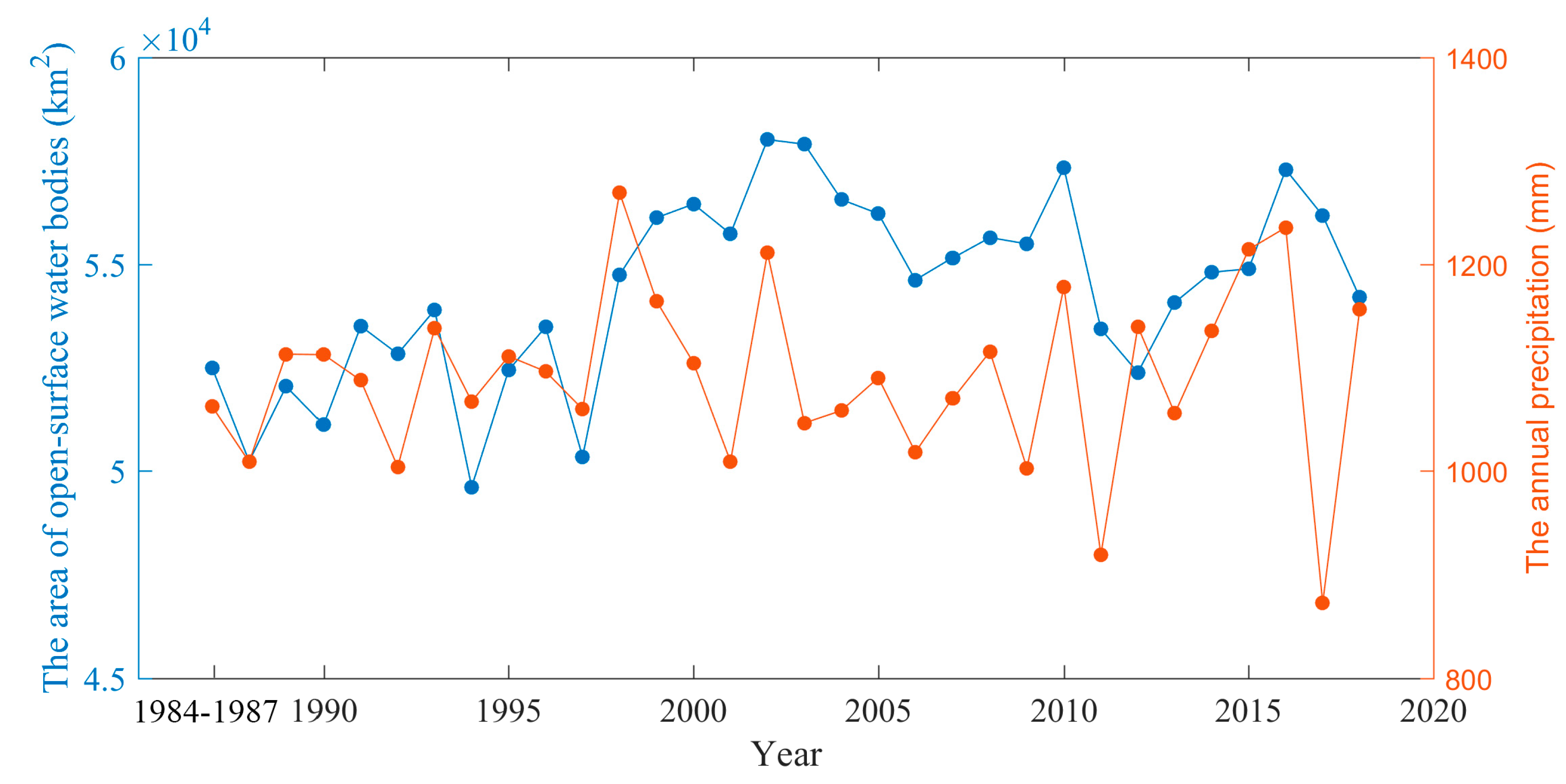
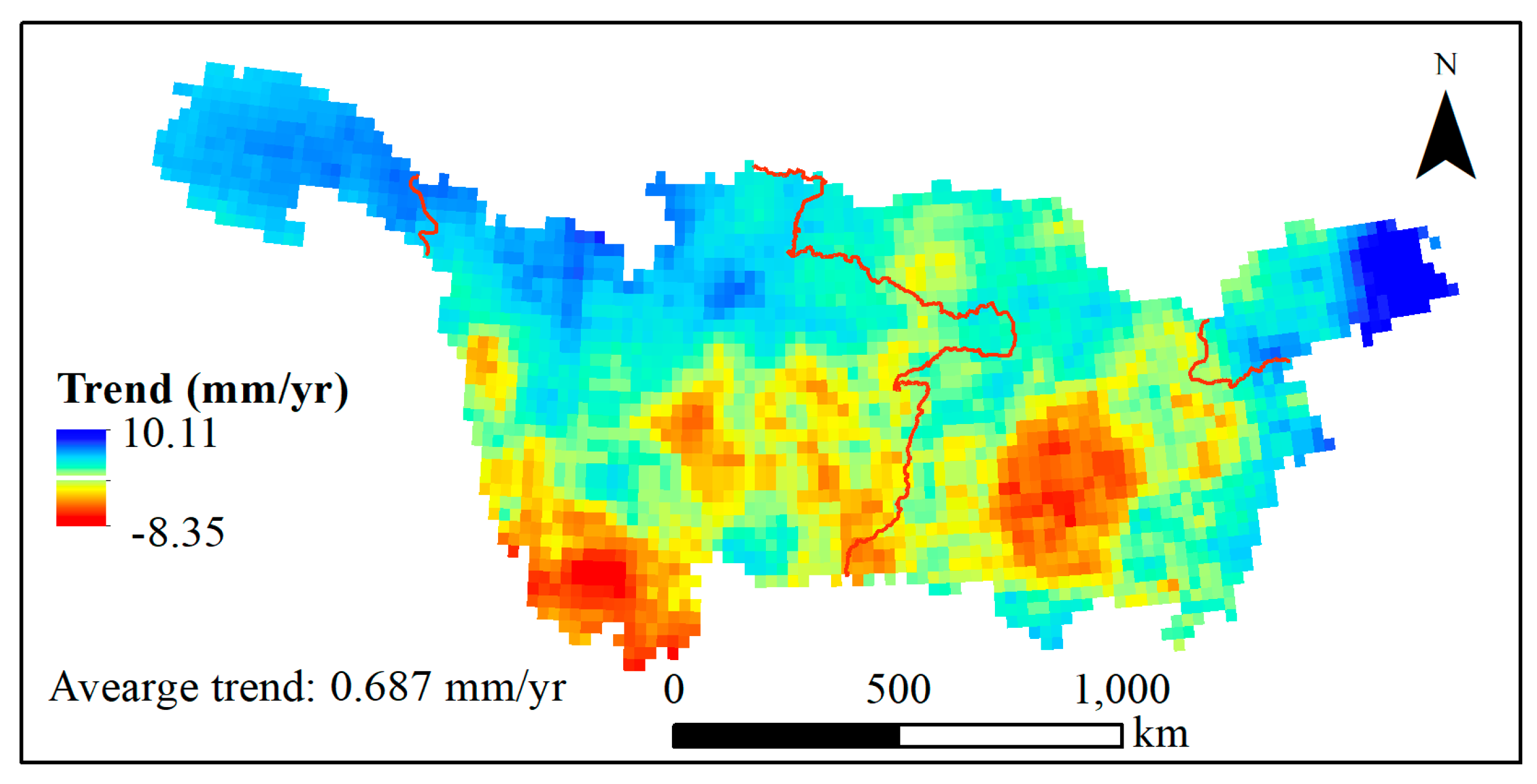
3.6. The Changes of Yearly Maximum Water Bodies and their Relationship with Precipitations in the YRB
4. Discussion
4.1. Changes in Open-Surface Water Bodies due to Climate and Human Factors
4.2. Long-Term and Large-Scale Mapping of Open-Surface Water Bodies by GEE Platform
4.3. Uncertainty and Prospects
5. Conclusions
Supplementary Materials
Author Contributions
Funding
Acknowledgments
Conflicts of Interest
References
- Costanza, R.; d’Arge, R.; De Groot, R.; Farber, S.; Grasso, M.; Hannon, B.; Limburg, K.; Naeem, S.; O’Neill, R.V.; Paruelo, J.; et al. The value of the world’s ecosystem services and natural capital. Nature 1997, 387, 253. [Google Scholar] [CrossRef]
- Wood, E.F.; Roundy, J.K.; Troy, T.J.; van Beek, L.P.H.; Bierkens, M.F.P.; Blyth, E.; de Roo, A.; Döll, P.; Ek, M.; Famiglietti, J.; et al. Hyperresolution global land surface modeling: Meeting a grand challenge for monitoring Earth’s terrestrial water. Water Resour. Res. 2011, 47. [Google Scholar] [CrossRef]
- Pekel, J.-F.; Cottam, A.; Gorelick, N.; Belward, A.S. High-resolution mapping of global surface water and its long-term changes. Nature 2016, 540, 418–422. [Google Scholar] [CrossRef] [PubMed]
- Jiang, Y. China’s water scarcity. J. Environ. Manag. 2009, 90, 3185–3196. [Google Scholar] [CrossRef] [PubMed]
- Khandelwal, A.; Karpatne, A.; Marlier, M.E.; Kim, J.; Lettenmaier, D.P.; Kumar, V. An approach for global monitoring of surface water extent variations in reservoirs using MODIS data. Remote Sens. Environ. 2017, 202, 113–128. [Google Scholar] [CrossRef]
- Li, L.; Vrieling, A.; Skidmore, A.; Wang, T.; Turak, E. Monitoring the dynamics of surface water fraction from MODIS time series in a Mediterranean environment. Int. J. Appl. Earth Obs. Geoinf. 2018, 66, 135–145. [Google Scholar] [CrossRef]
- Lu, S.; Jia, L.; Zhang, L.; Wei, Y.; Baig, M.H.A.; Zhai, Z.; Meng, J.; Li, X.; Zhang, G. Lake water surface mapping in the Tibetan Plateau using the MODIS MOD09Q1 product. Remote Sens. Lett. 2017, 8, 224–233. [Google Scholar] [CrossRef]
- Ranghetti, L.; Busetto, L.; Crema, A.; Fasola, M.; Cardarelli, E.; Boschetti, M. Testing estimation of water surface in Italian rice district from MODIS satellite data. Int. J. Appl. Earth Obs. Geoinf. 2016, 52, 284–295. [Google Scholar] [CrossRef]
- Zhang, Y.; Shi, K.; Zhou, Y.; Liu, X.; Qin, B. Monitoring the river plume induced by heavy rainfall events in large, shallow, Lake Taihu using MODIS 250m imagery. Remote Sens. Environ. 2016, 173, 109–121. [Google Scholar] [CrossRef]
- Che, X.; Feng, M.; Sexton, J.; Channan, S.; Sun, Q.; Ying, Q.; Liu, J.; Wang, Y. Landsat-Based Estimation of Seasonal Water Cover and Change in Arid and Semi-Arid Central Asia (2000–2015). Remote Sens. 2019, 11, 1323. [Google Scholar] [CrossRef]
- Jia, K.; Jiang, W.; Li, J.; Tang, Z. Spectral matching based on discrete particle swarm optimization: A new method for terrestrial water body extraction using multi-temporal Landsat 8 images. Remote Sens. Environ. 2018, 209, 1–18. [Google Scholar] [CrossRef]
- Li, L.; Chen, Y.; Xu, T.; Liu, R.; Shi, K.; Huang, C. Super-resolution mapping of wetland inundation from remote sensing imagery based on integration of back-propagation neural network and genetic algorithm. Remote Sens. Environ. 2015, 164, 142–154. [Google Scholar] [CrossRef]
- Tulbure, M.G.; Broich, M. Spatiotemporal patterns and effects of climate and land use on surface water extent dynamics in a dryland region with three decades of Landsat satellite data. Sci. Total Environ. 2019, 658, 1574–1585. [Google Scholar] [CrossRef] [PubMed]
- Wang, X.; Xie, S.; Zhang, X.; Chen, C.; Guo, H.; Du, J.; Duan, Z. A robust Multi-Band Water Index (MBWI) for automated extraction of surface water from Landsat 8 OLI imagery. Int. J. Appl. Earth Obs. Geoinf. 2018, 68, 73–91. [Google Scholar] [CrossRef]
- Hardy, A.; Ettritch, G.; Cross, D.E.; Bunting, P.; Liywalii, F.; Sakala, J.; Silumesii, A.; Singini, D.; Smith, M.; Willis, T.; et al. Automatic Detection of Open and Vegetated Water Bodies Using Sentinel 1 to Map African Malaria Vector Mosquito Breeding Habitats. Remote Sens. 2019, 11, 593. [Google Scholar] [CrossRef]
- Schwatke, C.; Scherer, D.; Dettmering, D. Automated Extraction of Consistent Time-Variable Water Surfaces of Lakes and Reservoirs Based on Landsat and Sentinel-2. Remote Sens. 2019, 11, 1010. [Google Scholar] [CrossRef]
- Steinhausen, M.J.; Wagner, P.D.; Narasimhan, B.; Waske, B. Combining Sentinel-1 and Sentinel-2 data for improved land use and land cover mapping of monsoon regions. Int. J. Appl. Earth Obs. Geoinf. 2018, 73, 595–604. [Google Scholar] [CrossRef]
- Wang, C.; Jia, M.; Chen, N.; Wang, W. Long-Term Surface Water Dynamics Analysis Based on Landsat Imagery and the Google Earth Engine Platform: A Case Study in the Middle Yangtze River Basin. Remote Sens. 2018, 10, 1635. [Google Scholar] [CrossRef]
- Gorelick, N.; Hancher, M.; Dixon, M.; Ilyushchenko, S.; Thau, D.; Moore, R. Google Earth Engine: Planetary-scale geospatial analysis for everyone. Remote Sens. Environ. 2017, 202, 18–27. [Google Scholar] [CrossRef]
- Mutanga, O.; Kumar, L. Google Earth Engine Applications. Remote Sens. 2019, 11, 591. [Google Scholar] [CrossRef]
- Oliphant, A.J.; Thenkabail, P.S.; Teluguntla, P.; Xiong, J.; Gumma, M.K.; Congalton, R.G.; Yadav, K. Mapping cropland extent of Southeast and Northeast Asia using multi-year time-series Landsat 30-m data using a random forest classifier on the Google Earth Engine Cloud. Int. J. Appl. Earth Obs. Geoinf. 2019, 81, 110–124. [Google Scholar] [CrossRef]
- Zurqani, H.A.; Post, C.J.; Mikhailova, E.A.; Schlautman, M.A.; Sharp, J.L. Geospatial analysis of land use change in the Savannah River Basin using Google Earth Engine. Int. J. Appl. Earth Obs. Geoinf. 2018, 69, 175–185. [Google Scholar] [CrossRef]
- Liu, X.; Hu, G.; Chen, Y.; Li, X.; Xu, X.; Li, S.; Pei, F.; Wang, S. High-resolution multi-temporal mapping of global urban land using Landsat images based on the Google Earth Engine Platform. Remote Sens. Environ. 2018, 209, 227–239. [Google Scholar] [CrossRef]
- Dong, J.; Xiao, X.; Menarguez, M.A.; Zhang, G.; Qin, Y.; Thau, D.; Biradar, C.; Moore, B. Mapping paddy rice planting area in northeastern Asia with Landsat 8 images, phenology-based algorithm and Google Earth Engine. Remote Sens. Environ. 2016, 185, 142–154. [Google Scholar] [CrossRef] [Green Version]
- Tang, Z.; Li, Y.; Gu, Y.; Jiang, W.; Xue, Y.; Hu, Q.; LaGrange, T.; Bishop, A.; Drahota, J.; Li, R. Assessing Nebraska playa wetland inundation status during 1985–2015 using Landsat data and Google Earth Engine. Environ. Monit. Assess. 2016, 188, 654. [Google Scholar] [CrossRef]
- Hird, J.; DeLancey, E.; McDermid, G.; Kariyeva, J.; Hird, J.N.; DeLancey, E.R.; McDermid, G.J.; Kariyeva, J. Google Earth Engine, Open-Access Satellite Data, and Machine Learning in Support of Large-Area Probabilistic Wetland Mapping. Remote Sens. 2017, 9, 1315. [Google Scholar] [CrossRef]
- Zhang, H.; Gorelick, S.M.; Zimba, P.V.; Zhang, X. A remote sensing method for estimating regional reservoir area and evaporative loss. J. Hydrol. 2017, 555, 213–227. [Google Scholar] [CrossRef]
- Zou, Z.; Xiao, X.; Dong, J.; Qin, Y.; Doughty, R.B.; Menarguez, M.A.; Zhang, G.; Wang, J. Divergent trends of open-surface water body area in the contiguous United States from 1984 to 2016. Proc. Natl. Acad. Sci. USA 2018, 115, 3810–3815. [Google Scholar] [CrossRef] [Green Version]
- Tulbure, M.G.; Broich, M.; Stehman, S.V.; Kommareddy, A. Surface water extent dynamics from three decades of seasonally continuous Landsat time series at subcontinental scale in a semi-arid region. Remote Sens. Environ. 2016, 178, 142–157. [Google Scholar] [CrossRef]
- Mcfeeters, S.K. The use of the Normalized Difference Water Index (NDWI) in the delineation of open water features. Int. J. Remote Sens. 1996, 17, 1425–1432. [Google Scholar] [CrossRef]
- Xu, H. Modification of normalised difference water index (NDWI) to enhance open water features in remotely sensed imagery. Int. J. Remote Sens. 2006, 27, 3025–3033. [Google Scholar] [CrossRef]
- Feyisa, G.L.; Meilby, H.; Fensholt, R.; Proud, S.R. Automated Water Extraction Index: A new technique for surface water mapping using Landsat imagery. Remote Sens. Environ. 2014, 140, 23–35. [Google Scholar] [CrossRef]
- Gómez, C.; White, J.C.; Wulder, M.A. Optical remotely sensed time series data for land cover classification: A review. ISPRS J. Photogramm. Remote Sens. 2016, 116, 55–72. [Google Scholar] [CrossRef] [Green Version]
- Khatami, R.; Mountrakis, G.; Stehman, S.V. A meta-analysis of remote sensing research on supervised pixel-based land-cover image classification processes: General guidelines for practitioners and future research. Remote Sens. Environ. 2016, 177, 89–100. [Google Scholar] [CrossRef] [Green Version]
- Tucker, C.J. Red and photographic infrared linear combinations for monitoring vegetation. Remote Sens. Environ. 1979, 8, 127–150. [Google Scholar] [CrossRef] [Green Version]
- Huete, A.; Didan, K.; Miura, T.; Rodriguez, E.P.; Gao, X.; Ferreira, L.G. Overview of the radiometric and biophysical performance of the MODIS vegetation indices. Remote Sens. Environ. 2002, 83, 195–213. [Google Scholar] [CrossRef]
- Zhou, Y.; Dong, J.; Xiao, X.; Liu, R.; Zou, Z.; Zhao, G.; Ge, Q. Continuous monitoring of lake dynamics on the Mongolian Plateau using all available Landsat imagery and Google Earth Engine. Sci. Total Environ. 2019, 689, 366–380. [Google Scholar] [CrossRef]
- Han, X.; Chen, X.; Feng, L. Four decades of winter wetland changes in Poyang Lake based on Landsat observations between 1973 and 2013. Remote Sens. Environ. 2015, 156, 426–437. [Google Scholar] [CrossRef]
- Wang, Y.; Ma, J.; Xiao, X.; Wang, X.; Dai, S.; Zhao, B. Long-Term Dynamic of Poyang Lake Surface Water: A Mapping Work Based on the Google Earth Engine Cloud Platform. Remote Sens. 2019, 11, 313. [Google Scholar] [CrossRef]
- Wu, G.; Liu, Y. Mapping Dynamics of Inundation Patterns of Two Largest River-Connected Lakes in China: A Comparative Study. Remote Sens. 2016, 8, 560. [Google Scholar] [CrossRef]
- Rao, P.; Jiang, W.; Hou, Y.; Chen, Z.; Jia, K. Dynamic Change Analysis of Surface Water in the Yangtze River Basin Based on MODIS Products. Remote Sens. 2018, 10, 1025. [Google Scholar] [CrossRef]
- Cui, L.; Wang, L.; Lai, Z.; Tian, Q.; Liu, W.; Li, J. Innovative trend analysis of annual and seasonal air temperature and rainfall in the Yangtze River Basin, China during 1960–2015. J. Atmos. Sol. Terr. Phys. 2017, 164, 48–59. [Google Scholar] [CrossRef]
- Sun, Z.; Zhu, X.; Pan, Y.; Zhang, J.; Sun, Z.; Zhu, X.; Pan, Y.; Zhang, J. Assessing Terrestrial Water Storage and Flood Potential Using GRACE Data in the Yangtze River Basin, China. Remote Sens. 2017, 9, 1011. [Google Scholar] [CrossRef]
- Vermote, E.; Justice, C.; Claverie, M.; Franch, B. Preliminary analysis of the performance of the Landsat 8/OLI land surface reflectance product. Remote Sens. Environ. 2016, 185, 46–56. [Google Scholar] [CrossRef]
- Ashouri, H.; Hsu, K.-L.; Sorooshian, S.; Braithwaite, D.K.; Knapp, K.R.; Cecil, L.D.; Nelson, B.R.; Prat, O.P. PERSIANN-CDR: Daily Precipitation Climate Data Record from Multisatellite Observations for Hydrological and Climate Studies. Bull. Am. Meteorol. Soc. 2015, 96, 69–83. [Google Scholar] [CrossRef] [Green Version]
- Gong, P.; Wang, J.; Yu, L.; Zhao, Y.; Zhao, Y.; Liang, L.; Niu, Z.; Huang, X.; Fu, H.; Liu, S.; et al. Finer resolution observation and monitoring of global land cover: First mapping results with Landsat TM and ETM+ data. Int. J. Remote Sens. 2013, 34, 2607–2654. [Google Scholar] [CrossRef]
- Zhu, Z.; Wang, S.; Woodcock, C.E. Improvement and expansion of the Fmask algorithm: Cloud, cloud shadow, and snow detection for Landsats 4–7, 8, and Sentinel 2 images. Remote Sens. Environ. 2015, 159, 269–277. [Google Scholar] [CrossRef]
- Zhu, Z.; Woodcock, C.E.; Holden, C.; Yang, Z. Generating synthetic Landsat images based on all available Landsat data: Predicting Landsat surface reflectance at any given time. Remote Sens. Environ. 2015, 162, 67–83. [Google Scholar] [CrossRef]
- Donchyts, G.; Schellekens, J.; Winsemius, H.; Eisemann, E.; van de Giesen, N. A 30 m Resolution Surface Water Mask Including Estimation of Positional and Thematic Differences Using Landsat 8, SRTM and OpenStreetMap: A Case Study in the Murray-Darling Basin, Australia. Remote Sens. 2016, 8, 386. [Google Scholar] [CrossRef]
- Qiao, B.; Zhu, L.; Yang, R. Temporal-spatial differences in lake water storage changes and their links to climate change throughout the Tibetan Plateau. Remote Sens. Environ. 2019, 222, 232–243. [Google Scholar] [CrossRef]
- Song, C.; Huang, B.; Ke, L.; Richards, K.S. Remote sensing of alpine lake water environment changes on the Tibetan Plateau and surroundings: A review. ISPRS J. Photogramm. Remote Sens. 2014, 92, 26–37. [Google Scholar] [CrossRef]
- Zhang, G.; Yao, T.; Xie, H.; Zhang, K.; Zhu, F. Lakes’ state and abundance across the Tibetan Plateau. Chin. Sci. Bull. 2014, 59, 3010–3021. [Google Scholar] [CrossRef]
- Wang, X.; Wang, W.; Jiang, W.; Jia, K.; Rao, P.; Lv, J. Analysis of the Dynamic Changes of the Baiyangdian Lake Surface Based on a Complex Water Extraction Method. Water 2018, 10, 1616. [Google Scholar] [CrossRef]
- Zhou, Y.; Ma, J.; Zhang, Y.; Li, J.; Feng, L.; Zhang, Y.; Shi, K.; Brookes, J.D.; Jeppesen, E. Influence of the three Gorges Reservoir on the shrinkage of China’s two largest freshwater lakes. Glob. Planet. Chang. 2019, 177, 45–55. [Google Scholar] [CrossRef]
- Deng, Y.; Jiang, W.; Tang, Z.; Li, J.; Lv, J.; Chen, Z.; Jia, K. Spatio-Temporal Change of Lake Water Extent in Wuhan Urban Agglomeration Based on Landsat Images from 1987 to 2015. Remote Sens. 2017, 9, 270. [Google Scholar] [CrossRef]


| Samples | Sentinel | Total | User’s Accuracy | ||
|---|---|---|---|---|---|
| Water | Non-Water | ||||
| Landsat | Water body | 5302 | 122 | 5424 | 97.75% |
| Non-water body | 325 | 3251 | 3576 | 90.91% | |
| Total | 4627 | 3373 | 9000 | Overall accuracy = 95.03% | |
| Producer’s accuracy | 94.22% | 96.38% | Kappa coefficient = 0.895 | ||
| Seasonal Water Bodies (km2) | Permanent Water Bodies (km2) | Total | |
|---|---|---|---|
| SYRB | 1670.21 | 2315.82 | 3986.03 |
| UYRB | 3023.91 | 3684.05 | 6707.96 |
| MYRB | 12,221.84 | 13,072.90 | 25,294.73 |
| LYRB | 4610.28 | 10,003.93 | 14,614.21 |
| YRB | 21,526.24 | 29,076.70 | 50,602.94 |
| Type | Area (km2) | Change Percentage (%) | ||
|---|---|---|---|---|
| 1984–1999 | 2000–2009 | 2010–2018 | 1984–2018 | |
| Seasonal water body | 17989.76 | 18576.06 | 16427.70 | −8.68% |
| Permanent water body | 29748.38 | 30654.89 | 32479.51 | 9.18% |
| Total | 47738.15 | 49230.94 | 48907.22 | 2.45% |
| Period | Maximum water bodies | Precipitation | Correlation |
|---|---|---|---|
| 1984–1999 | y = 215.74x + 51018; R2 = 0.199, P-value = 0.126 | y = 9.6832x + 1031.8; R2 = 0.302; P-value = 0.052 | R2 = 0.635; P-value = 0.019 |
| 2000–2009 | y = −204.78x + 57307; R2 = 0.314; P-value = 0.092 | y = −5.6389x + 1103.6; R2 = 0.075; P-value = 0.445 | R2 = 0.569; P-value = 0.086 |
| 2010–2018 | y = 105.74x + 54425; R2 = 0. 029; P-value = 0.659 | y = 2.036x + 1090.6; R2 = 0.002; P-value = 0.911 | R2 = 0.221; P-value = 0.568 |
| 2010–2018 (excluding 2012) | y = 20361x; R2 = 0.000; P-value = 0.964 | y = 2.7481x + 1083.5; R2 = 0.003; P-value = 0.853 | R2 = 0.351; P-value = 0.394 |
| 2000–2018 | y = −128187x; R2 = 0.185; P-value = 0.066 | y = 0.5296x + 1077; R2 = 0.001; P-value = 0.702 | R2 = 0.217; P-value = 0.372 |
| 2000–2018 (excluding 2012) | y = −103876x; R2 = 0.130; P-value = 0.077 | y = 1.1993x + 1071.5; R2 = 0.004; P-value = 0.758 | R2 = 0.338; P-value = 0.171 |
| 1984–2018 | y = 129.31x + 52218; R2 = 0.292; P-value = 0.001 | y = 0.3669x + 1085.4; R2 = 0.002; P-value = 0.827 | R2 = 0.207; P-value = 0.256 |
© 2019 by the authors. Licensee MDPI, Basel, Switzerland. This article is an open access article distributed under the terms and conditions of the Creative Commons Attribution (CC BY) license (http://creativecommons.org/licenses/by/4.0/).
Share and Cite
Deng, Y.; Jiang, W.; Tang, Z.; Ling, Z.; Wu, Z. Long-Term Changes of Open-Surface Water Bodies in the Yangtze River Basin Based on the Google Earth Engine Cloud Platform. Remote Sens. 2019, 11, 2213. https://doi.org/10.3390/rs11192213
Deng Y, Jiang W, Tang Z, Ling Z, Wu Z. Long-Term Changes of Open-Surface Water Bodies in the Yangtze River Basin Based on the Google Earth Engine Cloud Platform. Remote Sensing. 2019; 11(19):2213. https://doi.org/10.3390/rs11192213
Chicago/Turabian StyleDeng, Yue, Weiguo Jiang, Zhenghong Tang, Ziyan Ling, and Zhifeng Wu. 2019. "Long-Term Changes of Open-Surface Water Bodies in the Yangtze River Basin Based on the Google Earth Engine Cloud Platform" Remote Sensing 11, no. 19: 2213. https://doi.org/10.3390/rs11192213