Hyperspectral Sea Ice Image Classification Based on the Spectral-Spatial-Joint Feature with Deep Learning

Abstract

Sea ice is one of the causes of marine disasters. The classification of sea ice images is an important part of sea ice detection. The labeled samples in hyperspectral sea ice image classification are difficult to acquire, which causes minor sample problems. In addition, most of the current sea ice classification methods mainly use spectral features for shallow learning, which also limits further improvement of the sea ice classification accuracy. Therefore, this paper proposes a hyperspectral sea ice image classification method based on the spectral-spatial-joint feature with deep learning. The proposed method first extracts sea ice texture information by the gray-level co-occurrence matrix (GLCM). Then, it performs dimensionality reduction and a correlation analysis of the spectral information and spatial information of the unlabeled samples, respectively. It eliminates redundant information by extracting the spectral-spatial information of the neighboring unlabeled samples of the labeled sample and integrating the information with the spectral and texture data of the labeled sample to further enhance the quality of the labeled sample. Lastly, the three-dimensional convolutional neural network (3D-CNN) model is designed to extract the deep spectral-spatial features of sea ice. The proposed method combines relevant textural features and performs spectral-spatial feature extraction based on the 3D-CNN model by using a large amount of unlabeled sample information. In order to verify the effectiveness of the proposed method, sea ice classification experiments are carried out on two hyperspectral data sets: Baffin Bay and Bohai Bay. Compared with the CNN algorithm based on a single feature (spectral or spatial) and other CNN algorithms based on spectral-spatial features, the experimental results show that the proposed method achieves better sea ice classification (98.52% and 97.91%) with small samples. Therefore, it is more suitable for classifying hyperspectral sea ice images.

1. Introduction

Sea ice is an essential part of the Earth’s climate system [1] and one of the indicators of global climate change. It plays an important role in heat exchange between the ocean and the atmosphere [2]. Sea ice detection is very crucial for an accurate weather forecast [3]. At the same time, sea ice is one of the causes of marine disasters in polar and high mid-latitude regions. An unusually large flux of polar sea ice will disrupt the balance of freshwater [4], and affect the survival of living things [5]. Sea ice at a mid-high latitude affects the human marine fishery [6], coastal construction industry, and manufacturing industry, and also causes serious economic losses [7]. In recent years, sea ice disasters have attracted more attention. Sea ice detection has important research significance [8].

Sea ice detection needs to acquire effective data, and remote sensing technology has become an important means of analyzing and researching sea ice [9] because of its characteristics of timeliness, accuracy, and large-scale data acquisition. The sea ice detection data commonly used include passive microwave [10,11], synthetic aperture radar (SAR) [12,13], multispectral satellite images with a medium or high spatial resolution (MODIS) [14,15], Landsat [16], and hyperspectral images [17]. Of these, hyperspectral remote sensing data has a large amount of data and many bands. It can obtain continuous, high-resolution one-dimensional spectral information, and two-dimensional spatial information of a target object. Hyperspectral images (HSIs) have the characteristics of a “merged image-spectrum,” and provide important data support for accurate sea ice classification. However, the high dimensionality and large data volume of hyperspectral data bring many problems (e.g., a strong correlation among bands, mixed redundant pixels, and data information redundancy), which easily lead to the Hughes phenomenon and become a problem of sea ice detection. In recent years, hyperspectral remote sensing technology has been gradually applied to the research of sea ice detection. Common methods include the conventional minimum distance, maximum likelihood, decision tree [18], and the support vector machine (SVM) method [19], based on the iterative self-organizing data analysis technique algorithm (ISODATA) [20], linear prediction (LP) band selection [21], and more. However, most of the above methods only use the spectral information in HSIs. It is difficult to solve the phenomenon of “different objects with the same spectrum” in hyperspectral sea ice detection using only spectral information, and the introduction of effective spatial information can make up for the deficiency of using only spectral information [22], which can further improve the accuracy of sea ice classification. At present, the common spatial feature extraction methods are the gray-level co-occurrence matrix (GLCM) [23,24], Gabor filter [25], and morphological profiles (MPs) [26]. Among them, the statistical-based GLCM algorithm has a better application value because of its small feature dimension, strong discriminating ability, adaptability, and robustness [2,24]. However, these shallow and manual feature extraction methods based on expert experience and prior knowledge often ignore deep information, which limits the classification accuracy of HSIs.

In recent years, deep learning models have been well developed in the field of computer vision. Due to their characteristics from shallow to deep, from simple to complex, and independent of shallow artificial design, they can simultaneously extract the characteristics of deep spectral-spatial features, providing a new opportunity for the development of remote sensing technology. In 2014, for the first time in the field of remote sensing, an HSI classification method based on deep learning was introduced [27]. The method uses a stacked autoencoder (SAE) to extract the hierarchical and robust features of HSIs and achieved good results. Subsequently, a large number of deep learning algorithms for HSI classification were proposed. These algorithms make full use of the characteristics of deep learning, in order to learn nonlinear, discriminative, and invariant features from the data autonomously, such as the deep belief network (DBN) [28], the convolutional neural network (CNN) [29], etc. The focus has also evolved from spectral and spatial features to spectral-spatial-joint features. CNN, as a local connection network, automatically learns the features with translation invariance from the input data through the convolution kernel, combines the represented features with the corresponding categories for joint learning, and adaptively adjusts the features to get the best feature representation [30]. Additionally, hyperspectral data is usually represented by a three-dimensional data cube, which fits the input mode of extracting features from the three-dimensional convolution filter in CNN, and provides a simple and effective method for simultaneously extracting the features of spectral-spatial-combined features [31]. Therefore, in recent years, CNN has been widely used in the field of HSI classification.

It is well-known that deep learning algorithms acquire discriminative and robust feature representations in repeated iterative processes, which require long training time and a large number of training samples to achieve the purpose of accurately identifying the type of object [32]. Due to the particularity of the geographical environment of the sea ice covered area, it is difficult to obtain the actual land type information. It is necessary to manually label the sea ice type through prior knowledge. However, the labeling process is time consuming and costly. Due to the limited training samples and unpredictable sample quality, it is a challenge for deep learning algorithms to be applied to hyperspectral sea ice detection. To solve this problem, we improve the sample quality by combining the spectral-spatial information of unlabeled samples, reduce the cost of labeling, and realize sea ice detection based on deep learning using small samples. Therefore, our goal is to make full use of the spectral and spatial information of hyperspectral sea ice data and improve the accuracy of sea ice classification by using a deep learning method.

Based on the above research, this paper proposes a method for the classification of hyperspectral sea ice images based on spectral-spatial-joint features of deep learning, which combines three-dimensional CNN (3D-CNN) and the GLCM algorithm, enhances sample quality by making full use of the spectral-spatial information contained in neighboring, unlabeled samples of each pixel, and deep mines the spectral and spatial information of hyperspectral sea ice to further improve the accuracy of sea ice classification. Considering that 3D-CNN contains a large number of parameters to be trained, this paper utilizes the k-nearest neighbor (KNN) algorithm, which does not need any empirical parameters and is easy to implement, to select a certain number of unlabeled neighbor samples, and the information of unlabeled neighbor samples is used to enhance the quality of the labeled sample. However, the unlabeled sample also contains high-dimensional spectral information and redundant spatial information, which will burden the convolution operation of 3D-CNN. Therefore, in terms of the spectral information of unlabeled samples, based on our previous work [21], we adopt the dimensionality reduction algorithm to select the optimal spectral band combination, according to its spectral characteristics. Furthermore, in terms of spatial information, we remove the spatial features with a high redundancy by correlation analysis [33], and retain the low-correlation texture components for subsequent deep feature extraction, which reduces the burden of feature extraction in 3D-CNN as much as possible. Then, we compare the sea ice classification results with the existing National Snow and Ice Data Center (NSIDC, http://nsidc.org/) data to verify the reliability of the proposed method.

The remainder of this paper is organized as follows. Section 2 introduces the design framework and algorithm ideas in detail. The data set and related experimental setups are described in Section 3, and the effects of experimental results and related parameters are discussed in Section 4. Lastly, we summarize the work of this paper in Section 5.

2. Proposed Method

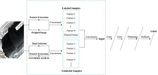
The framework of this proposed method is shown in Figure 1. It consists of four main parts: GLCM-based spatial feature extraction, unlabeled sample data processing based on the band selection algorithm and correlation analysis, labeled sample enhancement that fuses neighboring unlabeled samples’ information, and spectral-spatial feature extraction and classification based on the 3D-CNN. First, the spatial features are extracted from the original HSI using GLCM, and the extracted spatial features are merged with the original data as the labeled sample data. The unlabeled sample data is obtained from the original data and the extracted spatial features by using the band selection algorithm and correlation analysis. Lastly, the labeled sample data and the unlabeled sample data are fused as the input of 3D-CNN, and the study of deep space-spectral features is then carried out. This algorithm will be described in subsequent sections.

2.1. Feature Extraction: Gray Level Co-Occurrence Matrix (GLCM)

Texture is defined by the fact that the gray value of the pixel in the image changes continuously, according to a certain rule in the spatial position. It is one of the most important visual cues for identifying various homogeneous regions, which helps to segment or classify images [34].

A texture feature is a set of metrics computed by a feature extraction algorithm that is used to quantify the perceived texture of an image. Texture features are usually computed in a moving window, and each pixel in the image is set to an explicit and generic neighborhood set [26]. The GLCM method extracts the texture feature information of an image by counting the grayscale attributes of each pixel and its neighborhood in the image, which are statistics of the frequency at which two pixels with a certain gray value on the image appear under a given offset distance, which lists the joint probability distribution of the pixel pair at different gray values. It can be expressed as follows.

$$\begin{array}{l}p(i,j,d,\theta )=\{[(x,y),(x+D_x,y+D_y)|f(x,y)=i;\\ f(x+D_x,y+D_y)=j;x(y)=0,1,2,\dots ,N_{x(y)}]\}\end{array}.$$

(1)

In Equation (1), $i,j\in \{0,1,\dots ,N_g-1\}$ represents the set of $N_g$ quantized gray levels, d is the interval distance of pixel pairs, $\theta$ is the direction angle during the displacement process, $(x,y)$ is the relative coordinate of the pixel in the entire image, $D_x$ and $D_y$ are the horizontal and vertical offsets, respectively, and $N_x$ and $N_y$ are the columns and rows, respectively. $p(i,j,d,\theta )$ represents the number of times that the pixel pair appears on the direction angle $\theta$, where the gray values of the pixel pair are $i$ and $j$, respectively.

Generally, four angles of 0°, 45°, 90°, and 135° are taken in the process of calculating GLCM, and the values corresponding to $D_x$ and $D_y$ are $(1,0)$, $(0,1)$, $(1,1)$, and $(-1,1)$, respectively. Then, the eigenvalues in the four directions are averaged as a texture eigenvalue matrix.

The normalized gray level co-occurrence matrix can be expressed as follows.

$$P_{i,j}=\frac{p(i,j)}{R},R=\{\begin{array}{c}{N}_y(N_x-1)\\ (N_y-1)(N_x-1)\end{array}\begin{array}{c}\theta =0°\mathrm{or}\theta =90°\\ \theta =45°\mathrm{or}\theta =135°\end{array}.$$

(2)

In Equation (2), $P_{i,j}$ is the normalized representation of the elements in GLCM, $p(i,j)$ is an element $(i,j)$ of GLCM, and $N_x$ and $N_y$ are the columns and rows of the image, respectively. Normally, if the texture of the image is relatively uniform, the larger values of the GLCM extracted from the image are gathered near the diagonal. If the texture of the image changes more sharply, the larger value of the GLCM will be distributed farther from the diagonal.

In this paper, eight texture scalars are extracted by GLCM to form textural feature bands, i.e., mean, variance, homogeneity, contrast, dissimilarity, entropy, angular second moment, and correlation [24,33].

2.2. Band Selection

Hyperspectral data dimensionality reduction maximizes the retention of important information in the data while compressing the original data. Preserving less spectral bands by the band selection algorithm not only better preserves the original features of the band, but also removes interference from redundant information, which reduces the computational cost in CNN.

In the band selection part of the algorithm in this paper, we used the content of the improved similarity measurement method based on the linear prediction (ISMLP) algorithm considering our previous work [21]. The purpose of the algorithm is to select the optimal band combination with a great deal of information and low similarity between bands. The main idea is to determine the first initial band with the largest amount of information through mutual information (MI) and then select the second initial band by a spectral correlation measure (SCM). Then, subsequent band selection is performed by a linear prediction (LP) and the virtual dimension (VD) is used to estimate the minimum number of hyperspectral bands that should be selected.

2.3. 3D-CNN

Compared to one-dimensional convolutional neural network (1D-CNN) and two-dimensional convolutional neural network (2D-CNN) based on spectral features and spatial features, respectively, the 3D-CNN based on spectral-spatial-joint features takes into account the advantages of both and can simultaneously extract the spectral information and spatial information in HSI spontaneously. By initializing in an unsupervised manner, and then fine-tuning in a supervised manner, 3D-CNN constantly learns high-level features with abstraction and invariance from low-level features, which is conducive to classification, target detection, and other tasks.

In HSI classification, the 3D-CNN can map the input HSI pixels to the input pixel labels, so that each pixel in the HSI can obtain its category label through the network, and complete the pixel-level classification for HSI. In contrast, the 3D-CNN extracts the spectral-spatial information from the cube of the small spatial neighborhood centered on a certain pixel, and uses the category label obtained by the output layer as the label of the central pixel. Therefore, the input of the 3D-CNN is a three-dimensional cube block extracted from the HSI, and the pixel block size is K × K × B, where K is the spatial dimension of the pixel block and must be an odd number, and B is the size of the pixel block in the spectral dimension and is the number of bands of the HSI. The calculation formula for 3D-CNN is carried out as follows.

$${\upsilon }_{ij}^{xyz}=f({\displaystyle \sum _m{\displaystyle \sum _{h=0}^{H_i-1}{\displaystyle \sum _{w=0}^{W_i-1}{\displaystyle \sum _{r=0}^{R_i-1}{k}_{ijm}^{hwr}{\upsilon }_{(i-1)m}^{(x+h)(y+w)(z+r)}}}}}+b_{ij}).$$

(3)

where $R_i$ is the size of the 3D convolution kernel in the spectral dimension, $H_i$ and $W_i$, respectively, represent the height and width of the 3D convolution kernel, ${\upsilon }_{ij}^{xyz}$ is the value at the $j$th feature cube of the $i$th layer at the position $(x,y,z)$, $k_{ijm}^{hwr}$ represents the specific value of the $j$th convolution kernel of the $i$th layer at the position $(h,w,r)$, and the convolution kernel is connected to the $m$th feature cube of the $(i-1)$th layer, and $b_{ij}$ is biased while $f(•)$ is the activation function. In this paper, the ReLU function is used as the activation function, which is beneficial to gradient descent and back propagation, and avoids the problem of gradient disappearance. The formula is shown below.

$$f(x)=\mathrm{Re}LU(x)=\{\begin{array}{c}\begin{array}{cc}x& ifx>0\end{array}\\ \begin{array}{cc}0& ifx\le 0\end{array}\end{array}.$$

(4)

In addition, the Adaptive moment estimation (Adam) algorithm is used as the gradient optimization algorithm in this paper [35]. The algorithm combines the advantages of the adaptive gradient algorithm (AdaGrad) to deal with the sparse gradient and root mean square prop algorithm (RMSProp) to deal with non-stationary targets. The first-order moment estimation and second-order moment estimation of the gradient are used to dynamically adjust the learning rate of each parameter, after offset correction, and update the different parameters. The specific expression is as follows.

First, assume that, at time $t$, the first derivative of the objective function for the parameter is $g_t$. Equations (5) and (6) are updates to the biased first-order moment estimate and the biased second-order moment estimate of the gradient. The deviation is corrected according to the gradient by Equations (7) and (8), and, lastly, the parameter update is completed by Equation (9).

$$m_t={\beta }_1{m}_{t-1}+(1-{\beta }_1)g_t$$

(5)

$$v_t={\beta }_2{v}_{t-1}+(1-{\beta }_2)g_t^2$$

(6)

$$\stackrel{\wedge }{m_t}=m_t/(1-{\beta }_1^t)$$

(7)

$$\stackrel{\wedge }{v_t}=v_t/(1-{\beta }_2^t)$$

(8)

$${\theta }_{t+1}={\theta }_t-\eta ·\stackrel{\wedge }{m_t}/(\sqrt{\stackrel{\wedge }{v_t}}+\epsilon ).$$

(9)

In Equations (5)–(9), ${\beta }_1$ and ${\beta }_2$ are the exponential decay rates of the moment estimates, 0.9 and 0.999, respectively. $m_t$ and ${\nu }_t$ are first-order moments and second-order moment variables at time $t$, and the initial values are all 0 while $\eta$ is the learning rate. To prevent the denominator’s value being 0, the value of the small constant $\epsilon$ is set to ${10}^{-8}$, and ${\theta }_t$ is the 3D-CNN parameter variable at time $t$, including weights and offsets.

2.4. Implementation Process of the Proposed Method

According to the above algorithm, the specific algorithm implementation process is described as Algorithm 1 shown below.

Algorithm 1: Proposed Method

Begin

Input: Original HSIs

A. Feature extraction

(1) Process the original data set by the principal component analysis (PCA) algorithm, taking the first principal component (PC).

(2) According to the GLCM algorithm, slide the sliding window on the PC by step d and direction angle $\theta$, and calculate the gray level co-occurrence matrix of the sliding window every time it is slid, obtain the texture feature value, and then assign textural feature values to the center pixel of the window,

(3) Repeat (2) until the sliding window covers the PC,

(4) For a certain textural scalar, sum, and average the textural feature matrix of the four direction angles as the final textural feature matrix, and also do the same with other textural features,

(5) Repeat step (4) until eight textural features are obtained,

(6) Feature extraction is completed.

B. Nearest neighbor sample selection

(7) For a certain labeled sample in the original data, calculate the Euclidean distance with all unlabeled samples, and sorted into ascending order, its formula is as follows: $dist(x,y)=\sqrt{{\displaystyle \sum _{k=1}^n{(x_i-y_i)}^2}}$,

(8) Repeat step (7) until all labeled samples have been calculated,

(9) Neighbor samples extraction is completed.

C. Input data preprocessing

i. Labeled samples

(10) Stack the spatial features extracted from the phase with the original data.

(11) The data acquisition of labeled samples is completed.

ii. Unlabeled samples

(12) Obtain spectral features by reducing the original data by the band selection method in Section 2.2.

(13) Obtain spatial features by correlation analysis of the spatial features extracted from phase A, and remove the highly correlated components.

(14) Stack spectral features and spatial features in steps (12) and (13).

(15) The data acquisition of unlabeled samples is completed.

(16) Fuse the labeled sample data in i(Labeled samples) with the unlabeled sample data in ii(Unlabeled samples) according to the neighbor relationship in phase B.

(17) Input data is completed.

D. 3D-CNN

(18): Input data is randomly divided into training samples and test samples, and the input size of each sample is K × K × B.

Training stage

(19) Randomly select Batch (Batch = 20) training samples from the training samples into the pre-established 3D-CNN network each time.

(20) Suppose the first layer contains n convolution kernels of size C × C × D. After each K × K × B sample is subjected to the convolution operation of the first layer, n data cubes of size (K-C+1) × (K-C+1) × (B-D+1) are output values. The output of the first layer is the input of the second layer, which continues the convolution operation, and more. The final output is converted into a feature vector and then input into the fully connected layer, with the mapping and merging of local features extracted during convolution. After calculating the loss rate by the Softmax cross entropy function, the gradient of each parameter is calculated by back propagation, and the network parameters are dynamically updated by the Adam algorithm.

(21) Repeat steps (19) and (20), until the preset number of iterations is completed.

(22) Model training is completed.

Test stage

(23) Input the test sample in step (18) into the trained 3D-CNN model, and calculate the confusion matrix according to the predicted label and the real label to get the classification accuracy.

(24) Test is finished.

Output: confusion matrix, overall accuracy, average accuracy, Kappa statistic.

End

3. Experimental Results

To verify the effectiveness of the proposed method, we used two hyperspectral remote sensing sea ice datasets in the experiment. Baffin Bay images and Bohai Bay images were captured by the Earth Observation Satellite-1 (EO-1) [36], and compared with the other six algorithms: decision tree, SVM, 1D-CNN, 2D-CNN, 3D-CNN, and GLCM-CNN. GLCM-CNN combines the spatial features extracted by the GLCM with the original data, and then inputs the fused data into the CNN network. All classification algorithms used the overall accuracy (OA), average accuracy (AA), and kappa statistic (K) to evaluate the experimental results. Each algorithm ran the experiments 20 times with different initial random training samples. The classification accuracy values are given in the form of the mean ± standard deviation. The experimental environment is Intel(R) Core(TM) i5-2500 CPU 3.30 GHz and 22 GB Installed Memory.

3.1. Experiment in Baffin Bay

3.1.1. Data Description

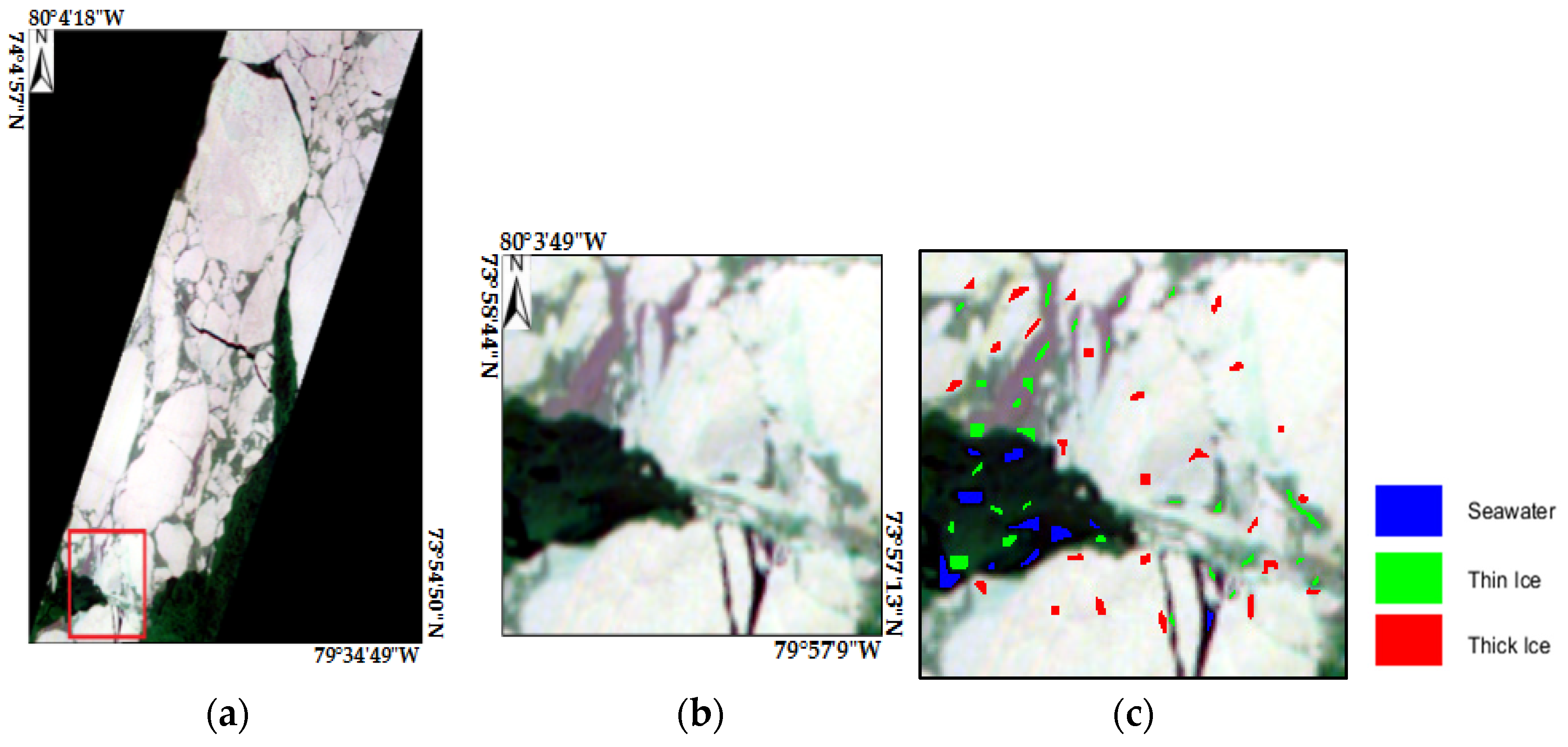
The first data used in this experiment is the Hyperion image without cloud coverage of the Baffin Bay near Greenland taken on 12 April, 2014. The latitude and longitude of the upper left-hand corner of the image are 79°51′27″ W and 74°16′16″ N, and the lower right-hand corner is located at 79°29′20″ W, 73°57′5″ N. The data set belongs to the level L1G, which is a level at which geometric correction, projection registration, and topographic correction have already been made [36]. The image size is 2395 pixels × 1769 pixels, with a spatial resolution of 30 m. Considering the computational cost, we take part of the original image as the experimental area, which contains all the sea ice categories in the original image. Additionally, the size of the experimental region is 186 pixels × 209 pixels. In the image data with 242 bands, after removing some of the low signal-noise-ratio (SNR) and water absorption bands, 176 bands were used for analysis [37]. According to the spectral characteristics of sea ice (see Figure 2) and NSIDC data (see Section 4.5), we divided the experimental scene into three categories: seawater, thin ice (<120 cm thick), and thick ice (>120 cm thick). By manually labeling a certain number of labeled samples as the sample database, which is taken as ground truth, the sample library was randomly divided into training samples and test samples, as shown in Figure 3 and

Table 1. Number of training samples (pixels) in each class for the Baffin Bay data set.

Class	Training	Test
Seawater	50	286
Thin Ice	50	361
Thick Ice	50	481
Total	150	1128

.

3.1.2. Experimental Setup

The CNN contains a large number of parameters to be trained. For 3D-CNN, the input size of the three-dimensional data (including the spatial dimension of the image and the size of the channel depth dimension) directly affects the training time of the model. As space dimensions increase and channel dimensions deepen, the time cost becomes higher. In order to reduce the time complexity of the model as much as possible, it is necessary to reduce the dimension of unlabeled samples containing spectral features and spatial features.

In terms of the spectral characteristics of unlabeled samples, based on our previous work [21], considering the information of the band itself, the similarity among the bands, and the spectral characteristics of the sea ice, we use the band selection algorithm to select a combination of bands with a large amount of information and low similarity among bands. Lastly, three bands are selected as the spectral features, and the band number is 16, 118, and 84, respectively.

In addition, correlation analysis methods are used to exclude highly correlated components of textural features extracted by GLCM. Quantitative analysis by the correlation matrix, shown in

Table 2. Correlation matrix for eight textural components in Baffin Bay data sets.

	Mea	Var	Hom	Con	Dis	Ent	ASM	Cor
Mea	1.0000	−0.1275	0.5493	−0.0661	−0.1443	−0.0847	0.4455	0.1698
Var	–	1.0000	−0.4669	0.0557	0.6084	0.4483	−0.3036	0.3194
Hom	–	–	1.0000	−0.0801	−0.5042	−0.5491	0.8020	−0.1178
Con	–	–	–	1.0000	0.7232	0.0684	−0.0480	−0.0074
Dis	–	–	–	–	1.0000	0.5641	−0.3968	0.3307
Ent	–	–	–	–	–	1.0000	−0.7353	0.6622
ASM	–	–	–	–	–	–	1.0000	−0.2421
Cor	–	–	–	–	–	–	–	1.0000
ABC	0.3234	0.4162	0.5087	0.2561	0.5340	0.5140	0.4967	0.3562

Mea: Mean. Var: Variance. Hom: Homogeneity. Con: Contrast. Dis: Dissimilarity. Ent: Entropy. ASM: Angular second moment. Cor: Correlation. ABC: Average absolute correlation.

, is the correlation of eight texture components in the Baffin Bay data set. When the two texture features are highly correlated (the absolute value of the correlation coefficient is greater than 0.7), the texture component with a smaller average absolute correlation is selected for further study. For example, in Table 2, the correlation coefficient between homogeneity and the angular second moment (ASM) is 0.8020, while the average absolute correlation of homogeneity is 0.5087, which is greater than ASM (0.4967). Similarly, the correlation coefficient between contrast and dissimilarity is 0.7232, the correlation coefficient between entropy and ASM is -0.7353, and contrast and entropy have a larger average absolute correlation. Therefore, five texture components are finally retained: mean, variance, contrast, ASM, and correlation.

Combining the three bands after band selection and the five texture components after correlation analysis, the eight attribute features are used to represent the unlabeled sample spectral-spatial information. Additionally, 20 neighbor samples (K = 20) are selected for the each labeled sample, and its spectral-spatial feature is used as the patch information of the labeled sample. The channel (depth) dimension of the final input data is 176 + 8 + 8 × 20 = 344. The model proposed in Reference [31] is lightweight and easy to train and adjust, and, in order to further reduce the time cost, this paper draws on the advantages of the model and optimizes it on the hyper-parameters. The model structure is shown in

Table 3. Network structure for the Baffin Bay data set.

Layer NO.	1	2	3
Kernel size	3 × 3 × 4	3 × 3 × 2	-
Strides	1 × 1 × 1	1 × 1 × 1	-
ReLU	Yes	Yes	-
Pooling	No	No	-
Dropout	No	No	Yes
Filters	2	4	120

. The model contains two convolutional layers, a fully connected layer, and an input layer and output layer. The data input size is 5 × 5 × 344 and this is normalized to [0, 1]. The learning rate is set to 0.001 and the dropout value is 0.5. The number of training iterations is 2000, and 20 training samples are randomly input into the network for each iteration.

3.1.3. Experimental Results and Discussion

Table 4. Classification results (%) of the Baffin Bay data set.

	Decision Tree	SVM	1D-CNN	2D-CNN	3D-CNN	GLCM-CNN	Proposed
OA	85.54 ± 0.4235	90.36 ± 1.1913	89.78 ± 2.1923	93.47 ± 1.5564	95.44 ± 0.9099	96.02 ± 0.9497	98.52 ± 0.5670
AA	86.04 ± 0.4617	90.37 ± 0.9152	89.22 ± 2.9058	93.92 ± 1.5596	94.81 ± 2.3071	96.25 ± 0.8373	98.60 ± 0.8692
K×100	78.25 ± 0.6272	85.31 ± 1.7706	84.47 ± 3.2756	90.03 ± 2.3588	93.03 ± 1.3917	93.91 ± 1.4447	97.73 ± 0.5186
Seawater	94.90 ± 1.6250	92.73 ± 2.7074	93.53 ± 1.9933	97.55 ± 2.6231	99.20 ± 1.1185	99.76 ± 0.3704	99.72 ± 0.4603
Thin Ice	65.46 ± 1.5026	82.27 ± 3.9080	82.37 ± 5.6011	91.36 ± 3.1526	88.52 ± 5.5343	93.13 ± 2.4212	97.70 ± 1.3699
Thick Ice	97.84 ± 0.9761	96.15 ± 2.6916	91.58 ± 5.1144	93.01 ± 1.9009	96.76 ± 1.9434	96.13 ± 2.1409	98.46 ± 0.9662

* The bold style represents the highest accuracy among the compared methods.

shows the classification results of the Baffin Bay data set based on different classification methods. The classification result values are obtained by comparing the prediction label and the corresponding ground truth. In the experiment, the input sizes of 2D-CNN and 3D-CNN are 19 × 19 and 5 × 5 × 176, respectively. The input size of GLCM-CNN is 5 × 5 × (176 + 8), where 176 is the original band number and 8 are the eight texture components extracted from the first principal component by GLCM. It can be seen from Table 4 that, compared with other algorithms, the proposed algorithm achieves the best classification result, and the OA is 98.52%. As can be seen, as a whole, decision tree and SVM achieve relatively low classification accuracy (85.54% and 90.36%, respectively) because SVM and decision tree belong to a shallow learning model, and do not fully mine the spatial features in the process of classification. Compared with 1D-CNN using only spectral features and 2D-CNN using only spatial features, the increase is 8.74% and 5.05%, respectively, which indicates that the use of spectral-spatial-joint features can effectively improve the accuracy of sea ice classification. In the method based on spectral-spatial features, GLCM-CNN is higher than 3D-CNN, which reflects the validity of the texture information extracted by GLCM. However, the accuracy improvement is limited, with a value of only 0.58%. The proposed method is 3.08% higher than 3D-CNN and 2.50% higher than the GLCM-CNN result (96.02%) with unfused neighbor sample information, and AA and the Kappa coefficient are increased by 2.35% and 3.82%, respectively. It is proved that the spatial information of the unlabeled samples of the nearest neighbors can effectively enhance the quality of training samples and improve the accuracy of sea ice classification, which further proves the superiority of the proposed method.

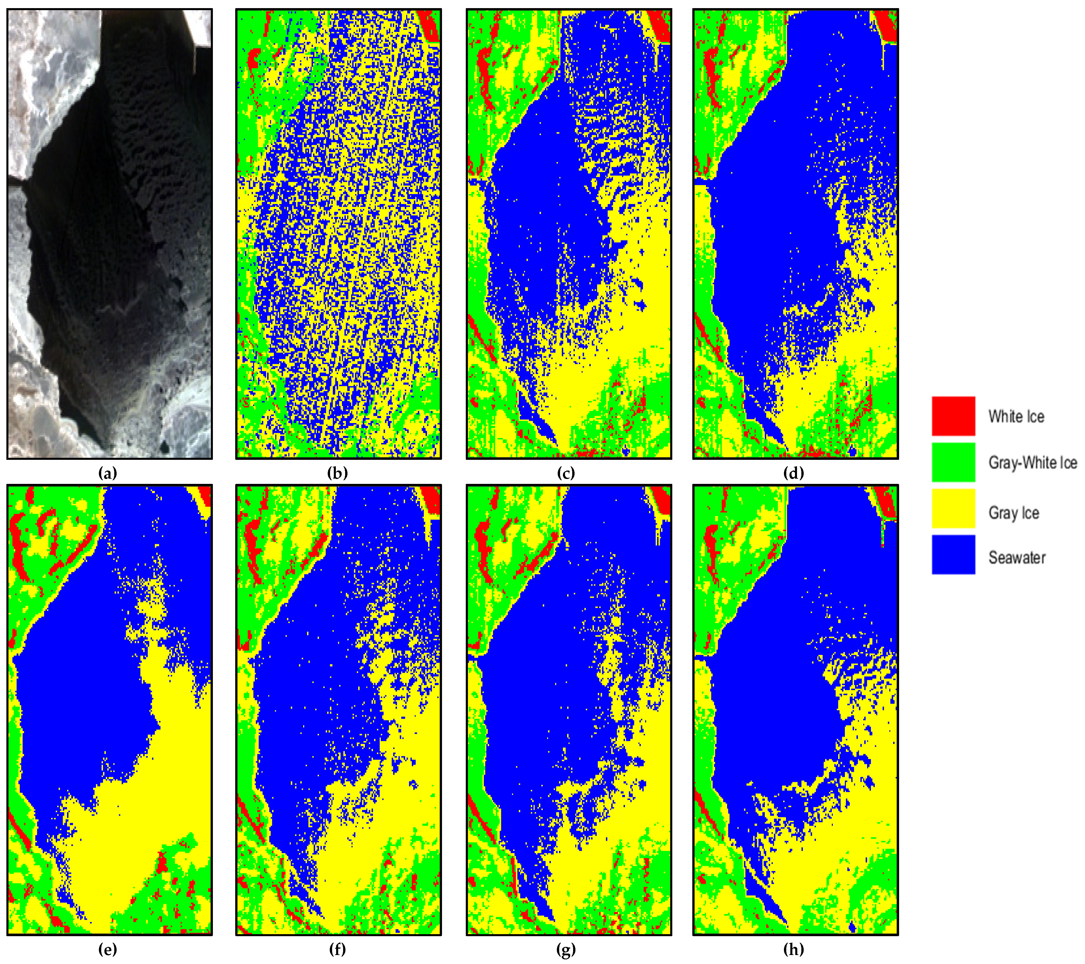
Among the three categories, Seawater has a lower reflectance of the spectrum due to its own characteristics, so it is more distinguishable than sea ice. Thin ice, as an intermediate category between seawater and thick ice, has a wide range of thicknesses, so its misclassification is serious. In Table 4, thin ice’s classification accuracy in the seven methods is relatively low, and it is difficult to distinguish by spectral features in the decision tree, SVM, and 1D-CNN. In 2D-CNN and GLCM-CNN, the classification of thin ice by spatial features has obtained certain effects. The proposed method fuses the spatial information of the unlabeled neighbor samples based on the spatial features of the original labeled samples, and obtains the best classification results, which are increased by 6.34% and 4.57%, respectively. The classification result images are shown in Figure 4. Because the proposed method has advantages for the classification of intermediate categories (thin ice), the visual classification results are more accurate for the category boundaries.

3.2. Experiment in Bohai Bay

3.2.1. Data Description

The second data used in this experiment is the Hyperion image without cloud coverage of the Bohai Bay region taken on 23 January, 2008. The latitude and longitude of the upper left-hand corner of the image are 120°45′12″W and 41°39′7″N, and the lower right-hand corner is located at 121°13′9″E, 39°44′42″N. The image size is 7061 pixels × 2001 pixels and the spatial resolution is 30 m. The scene covered by sea ice is cut out from the original image as the experimental area. After clipping, the size of the experimental area is 272 pixels × 159 pixels. Similar to the Baffin Bay data, 176 bands were selected for analysis in 242 bands, and the experimental areas are classified into four categories, according to spectral characteristics (see Figure 5) and NSIDC data (see Section 4.5). white ice (30–70 cm thick), gray-white ice (15–30 cm thick), gray ice (10–15 cm thick), and seawater. Labeled samples were acquired by manual labeling and then randomly divided into training samples and test samples in a 1:1 ratio, as shown in Figure 6 and

Table 5. Number of training samples (pixels) in each class for the Bohai Bay data set.

Class	Training	Test
White ice	219	219
Gray-white ice	350	350
Gray ice	325	326
Seawater	133	134
Total	1027	1029

.

3.2.2. Experimental Setup

For the Bohai Bay data set, band 21, band 120, and band 83 were selected as the optimal combined bands to represent the spectral information of the unlabeled samples [21].

Table 6. Correlation matrix for eight textural components in Bohai Bay data sets.

	Mea	Var	Hom	Con	Dis	Ent	ASM	Cor
Mea	1.0000	0.3969	−0.6125	0.4204	0.7458	0.7358	−0.5007	0.3265
Var	–	1.0000	−0.3760	0.5909	0.7148	0.3634	−0.2353	0.3867
Hom	–	–	1.0000	−0.3730	−0.6237	−0.5151	0.7914	−0.0100
Con	–	–	–	1.0000	0.8214	0.3649	−0.2374	0.2328
Dis	–	–	–	–	1.0000	0.7219	−0.4881	0.3672
Ent	–	–	–	–	–	1.0000	−0.7158	0.3321
ASM	–	–	–	–	–	–	1.0000	0.0608
Cor	–	–	–	–	–	–	–	1.0000
ABC	0.5932	0.5080	0.5377	0.5051	0.6854	0.5940	0.5040	0.3395

Mea: Mean. Var: Variance. Hom: Homogeneity. Con: Contrast. Dis: Dissimilarity. Ent: Entropy. ASM: Angular second moment. Cor: Correlation. ABC: Average absolute correlation.

is the correlation matrix of the Bohai Bay data set, in which the correlation coefficients of mean and dissimilarity, and entropy are 0.7458 and 0.7358, respectively. The mean’s average absolute correlation (0.5932) is lower than that of the two texture components. Therefore, dissimilarity and entropy are excluded. Homogeneity is highly correlated with the angular second moment, when comparing the average absolute correlation of them (0.5377 and 0.5040) and excluding homogeneity. According to Table 6, five texture components are retained, which are mean, variance, contrast, ASM, and correlation.

The input data of the Bohai Bay data set is 5 × 5 × 344, where 334 contains the original 176 bands of the input sample and its texture feature band, and the patch information. Additionally, for the patch information, each nearest neighbor sample contains the optimal band combination of three bands and five low-correlation texture components.

Table 7. Network structure for the Bohai Bay data set.

Layer NO.	1	2	3
Kernel size	3 × 3 × 8	3 × 3 × 3	-
Strides	1 × 1 × 1	1 × 1 × 1	-
ReLU	Yes	Yes	-
Pooling	No	No	-
Dropout	No	No	Yes
Filters	2	4	152

shows its model network structure, normalizing the input data to [0, 1], and other hyper-parameter settings are the same as the Baffin Bay data set.

3.2.3. Experimental Results and Discussion

The classification results and result maps of the Bohai Bay data set are shown in

Table 8. Classification results (%) of the Bohai Bay data set.

	Decision Tree	SVM	1D-CNN	2D-CNN	3D-CNN	GLCM-CNN	Proposed
OA	83.87 ± 1.5408	89.61 ± 2.0127	90.59 ± 1.3822	94.08 ± 1.2518	94.95 ± 1.4046	96.43 ± 1.5201	97.91 ± 0.4788
AA	79.20 ± 0.8478	90.44 ± 1.7748	91.83 ± 1.0428	94.34 ± 1.5949	95.41 ± 1.2995	96.98 ± 1.1425	98.28 ± 0.4042
K×100	77.73 ± 1.9795	85.34 ± 2.8801	87.00 ± 1.8699	91.74 ± 1.7634	92.99 ± 1.9418	95.06 ± 2.0986	97.11 ± 0.6624
White Ice	98.59 ± 0.3980	87.86 ± 3.7912	89.00 ± 6.8091	89.76 ± 6.1591	92.33 ± 4.0716	96.89 ± 2.2963	98.90 ± 1.1829
Gray-White Ice	97.17 ± 1.1305	87.03 ± 3.7233	87.51 ± 4.8749	93.97 ± 2.9591	93.97 ± 3.2281	95.43 ± 2.4908	97.20 ± 1.5982
Gray Ice	75.31 ± 5.5803	90.98 ± 2.9783	91.32 ± 3.1384	94.28 ± 1.9683	95.92 ± 2.9210	95.83 ± 3.6128	97.24 ± 1.2523
Seawater	45.75 ± 5.1349	95.90 ± 1.9026	99.48 ± 0.9981	99.33 ± 1.4268	99.40 ± 1.1561	99.78 ± 0.5037	99.78 ± 0.3605

* The bold style represents the highest accuracy among the compared methods.

and Figure 7. Among the four comparison algorithms, the input of the 3D-CNN is 9 × 9 × 176, and the others are the same as the Baffin Bay data set. The proposed method has the same spatial dimension as GLCM-CNN, and both of them are 5 × 5. From Table 8, the proposed method obtains the highest classification accuracy (OA = 97.91%), which is 14.04%, 8.30%, 7.32%, 3.83%, 2.96%, and 1.48% higher than the decision tree (83.87%), SVM (89.61%), 1D-CNN (90.59%), 2D-CNN (94.08%), 3D-CNN (94.92%), and GLCM-CNN (96.43%), respectively. This indicates that, when the spatial dimension input size is not very different, the proposed method is effective in extracting spatial information from the nearest unlabeled, neighbor samples to enhance the sample quality. In the seawater and three sea ice categories, the proposed method has an advantage in classifying the intermediate category (gray-white ice and gray ice). Compared with 2D-CNN, 3D-CNN, and GLCM-CNN, which contain spatial information, in the proposed method, the classification accuracy of gray-white ice increased by 3.23%, 3.23%, and 1.77%, respectively, and that of gray ice increased by 2.96%, 1.32%, and 1.41%, respectively. Moreover, as demonstrated by the classification result map, the proposed method effectively eliminates noise points. The classification result map is smoother and the distinction between different types of edge regions is more precise.

4. Discussion

4.1. Training Samples

The number of training samples is a very important factor in CNN training. Since CNN contains many parameters to be trained, a large number of training samples are needed to ensure the diversity of samples and to extract more robust and effective features. For sea ice at different latitudes, we explored the number of training samples separately. Additionally, 10 experiments were carried out under different training sample sizes, and the classification accuracy value was the average of 10 experimental results. For the Baffin Bay data set, which is located in the high latitudes of the Arctic, different types of sea ice have greater distinction. We only need fewer training samples to achieve a higher classification accuracy. This paper randomly selects the same number of training samples for different categories. As shown in Figure 8a, the classification accuracy increases with the training sample number, but the proposed method in this paper is superior to other algorithms under different training sample sizes. For example, when only 10 training samples are selected for each category, the average precision of the 10 experiments under random sampling is 90.34%, compared with the decision tree (84.91%), SVM (79.75%), 1D-CNN (81.37%), 2D-CNN (81.32%), 3D-CNN (84.89%), and GLCM-CNN (87.72%), which increased by 5.43%, 10.59%, 8.97%, 9.02%, 5.45%, and 2.62%, respectively. When the number of training samples for each category is 20, the difference between the other four methods reaches the maximum, which is 9.60%, 11.38%, 10.59%, 9.60%, 5.36%, and 3.25%, respectively.

Compared to Baffin Bay, Bohai Bay is in a mid-latitude and mainly contains one year ice. The separability between different types of sea ice is low, and more training samples are needed. Therefore, for the Bohai Bay data set, 10% to 50% of the training samples are randomly selected, and the rest are used as test samples. Ten experiments are performed at different scales. As shown in Figure 8b, the proposed method has advantages in different training sample ratios, especially when the training samples are insufficient. When the training sample ratio is 10%, the classification accuracy of the proposed approach is 92.74%. Compared with the decision tree (82.64%), SVM (65.33%), 1D-CNN (86.85%), 2D-CNN (88.72%), 3D-CNN (85.99%), and GLCM-CNN (89.13%), the proposed approach’s accuracies are increased by 10.10%, 27.41%, 5.89%, 4.02%, 6.75%, and 3.61%, respectively.

4.2. The Value of K

The KNN algorithm does not contain any parameters to be trained, and only the selection of the K value has an effect on the results. The K value represents the number of neighbor samples in the unlabeled sample. This section mainly explores the effect of the K value on the algorithm from 1 to 20 and performs five experiments under random sampling with different K values. As shown in Figure 9, as the K value increases, the classification accuracy value is on the rise, but the selected neighboring samples also increase. Although it brings a wealth of information to the labeled samples, it also means that the channel (depth) dimension of the input data increases, and it takes more time to train a robust and efficient classification model. Therefore, choosing the appropriate K value requires a comprehensive consideration of the impact on the classification accuracy and model computational complexity. In summary, in the experiment of this paper, the K values in both data sets are 20.

4.3. The Size of the GLCM Sliding Window

GLCM extracts spatial texture information through a sliding window of a certain size. The difference in sliding windows affects the extraction of features, and the computational cost increases as the window increases. In order to select the appropriate sliding window, this section selects 3 × 3, 5 × 5, and 7 × 7 as three sizes of windows for the two data sets to explore. It performs 10 experiments under different window sizes. The classification results are shown in

Table 9. Classification results (%) of the Baffin Bay data set with sliding windows of different sizes.

	3 × 3	5 × 5	7 × 7
OA	98.17 ± 0.9479	98.52 ± 0.5670	98.49 ± 0.9767
AA	98.38 ± 0.8538	98.60 ± 0.8692	98.63 ± 0.9189
K×100	97.19 ± 1.4485	97.73 ± 0.5186	97.69 ± 1.4970
Seawater	99.88 ± 0.2019	99.72 ± 0.4603	99.53 ± 0.8075
Thin Ice	96.25 ± 2.3768	97.70 ± 1.3699	94.85 ± 1.6888
Thick Ice	96.05 ± 1.4404	98.46 ± 0.9662	98.13 ± 1.7017

and

Table 10. Classification results (%) of the Bohai Bay data set with sliding windows of different sizes.

	3 × 3	5 × 5	7 × 7
OA	97.67 ± 0.6100	97.91 ± 0.4788	97.62 ± 0.4038
AA	98.14 ± 0.5260	98.28 ± 0.4042	98.00 ± 0.2954
K×100	96.78 ± 0.8436	97.11 ± 0.6642	96.70 ± 0.5585
White Ice	99.50 ± 0.4500	98.90 ± 1.1829	98.19 ± 1.1566
Gray-White Ice	95.69 ± 1.5501	97.20 ± 1.5982	96.69 ± 1.2211
Gray Ice	97.76 ± 2.2357	97.24 ± 1.2523	97.42 ± 1.1854
Seawater	99.63 ± 0.8061	99.78 ± 0.3605	99.70 ± 0.3854

. Both data sets achieve the highest precision in the sliding window 5 × 5, which is not much different from the results of the other two types of sliding windows. However, in the calculation, the larger the sliding window, the more edge samples are lost, which will affect the classification accuracy. Considering the balance between the classification accuracy and calculation time, in the Baffin Bay data set and the Bohai Bay data set, the sliding window size of the proposed method is 5 × 5.

4.4. Training Time

Table 11. Training time (minutes) for the two data sets for different methods.

	Decision Tree	SVM	1D-CNN	2D-CNN	3D-CNN	GLCM-CNN	Proposed
Baffin Bay	0.01	0.03	0.15	0.18	5.77	4.95	9.02
Bohai Bay	0.02	0.26	0.28	0.20	18.90	7.06	13.38

compares the training times of different algorithms for the two data sets. Because the shallow learning model is relatively simple, its training time is generally less than the deep learning method. The input size of the training data, the number of iterations, the amount of training samples input in batches, and the hyperparameters of the model (the number of convolutional layers, the size and number of convolution kernels, etc.) all have an impact on the training time. For example, in the Baffin Bay experiment, 3D-CNN has the same number of convolutional layers (two layers) and convolutional kernel size (3 × 3) as GLCM-CNN. Iterations are 2000 and batch size is 20 in both of them. However, the number of convolution kernels in each layer in 3D-CNN is 7 and 3, respectively, and the number of neurons in the fully connected layer is 256, which is 4, 2, and 120 in GLCM-CNN, respectively (select the best parameters based on the experimental results). In the case of the same input size, the channel (depth) dimension of GLCM-CNN is higher than 3D-CNN, but the number of convolution kernels in the model and the number of neurons in the fully connected layer are both smaller than 3D-CNN. Therefore, its training time is less than 3D-CNN. Due to the addition of texture information and unlabeled sample information increasing the computational complexity, the training time of the proposed method is increased when compared with other algorithms. A similar situation also appeared in the Bohai Bay experiment.

4.5. Method Validation

Because of the particularity of the geographical environment and condition, it is difficult to obtain the measured data of the sea ice covered area. In order to verify the effectiveness of the proposed method, we refer to the sea ice distribution vector data with the same-area and same-period downloaded from the National Snow and Ice Data Center (http://nsidc.org/) and make a qualitative verification. The downloaded data format is the Sea Ice Grid-3 (SIGRID-3), which contains the ice map (distribution by region) and the corresponding attribute list (such as the concentration, stage of development, and form of ice) [38].

The Baffin Bay experimental area in the paper is part of the red area in Figure 10a and the National Snow and Ice Data Center also provides the sea ice data description file [38] of the red area, as shown in Figure 10b.

The main parameter values are CT: 91, SA: 93, FA: 06, CN: 95, Poly_type: I, and the value “-9” represents no information.

As can be seen from

Table 12. Description of the main parameters.

CT	Total Concentration	90: 90%, 91: 90–100%, 92: 100%
SA	Stage of development of thickest ice	93: >120 cm
FA	Thick ice form corresponding to SA	05: Big floe 06: Vast floe
CN	Stage of development of ice thicker than SA but with concentration less than 1/10 density	93: Thick first year ice, 95: Old ice
POLY TYPE	Surface type	W: Water I: Ice

, the total sea ice concentration in the region is 90–100%. From the parameters SA and CN of the sea ice type, we can get the sea ice information: Vast Floe (>120 cm) and Old Ice. In our classification results, there are 35,778 classified pixels, of which 2394 are labeled as seawater, which accounts for 6.69% of the total. Therefore, our classification results are consistent with the data provided by the National Snow and Ice Data Center.

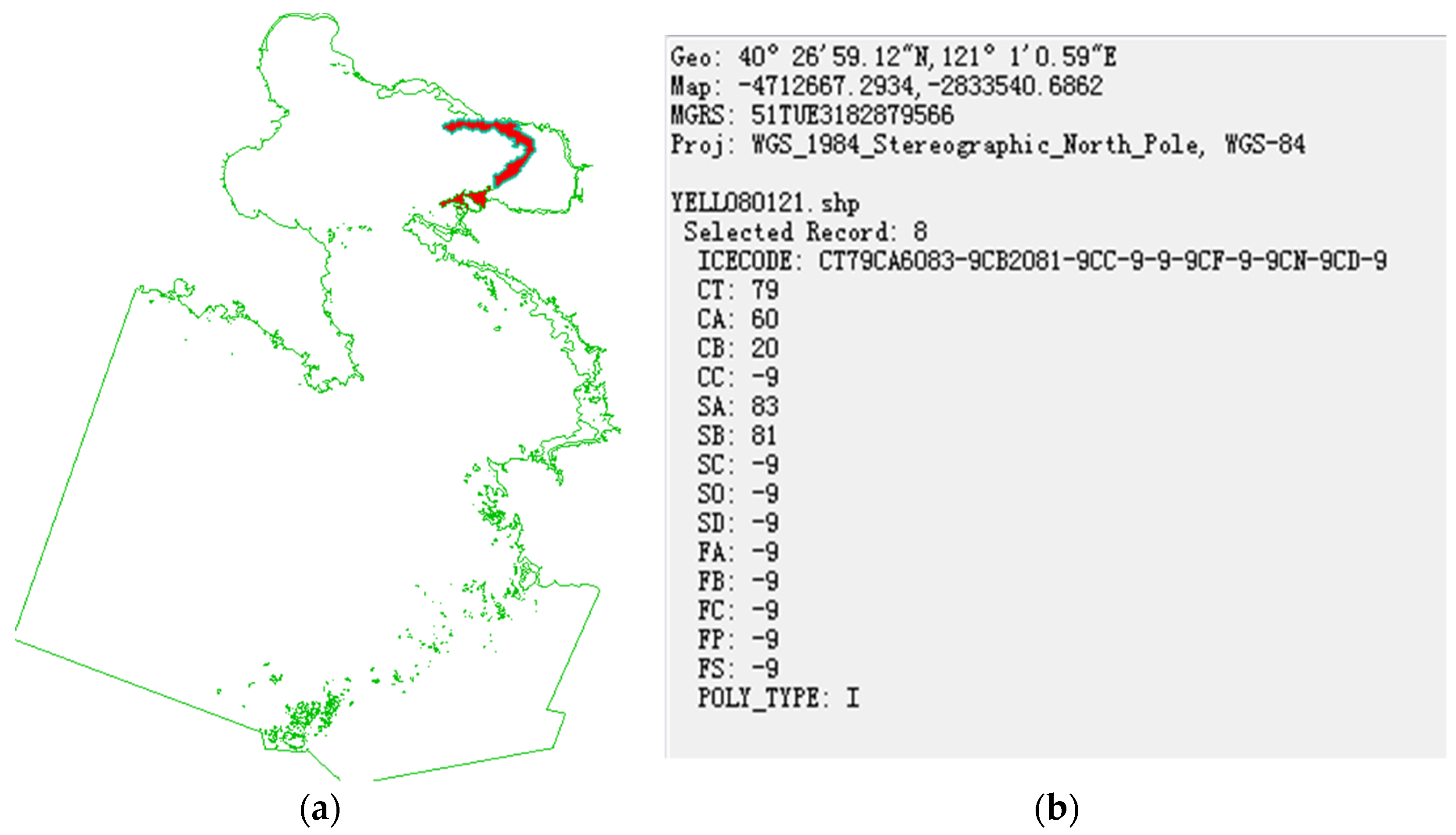
Figure 11a shows the sea ice distribution near Bohai Bay, and the red cover contains the experimental area. Figure 11b shows the sea ice parameters in the red area.

From Figure 11b, the main parameter values are: CT: 79, CA: 60, CB: 20, SA: 83, SB: 81, Poly_type: I. The parameters are described in

Table 13. Description of the main parameters.

CT	Total Concentration	70: 70%, 79: 70–90%, 80: 80%
CA	Partial concentration of thickest ice	60: 60%
CB	Partial concentration of second thickest ice	20: 20%
SA	Stage of development of thickest ice	83: Young ice (10–30 cm), 84: Gray ice (10–15 cm), 85: Gray-white ice (15–30 cm)
SB	Stage of development of second thickest ice	81: New ice
POLY TYPE	Surface type	W: Water. I: Ice

below.

The total sea ice concentration in the region is 70–90%, as can be seen from Table 13. From the parameters CA and SA, we can get the sea ice information: young ice (10–30 cm). In our classification results, there are 41,540 classified pixels, of which 20,759 are labeled as seawater. This means that the sea ice accounts for 50.03% of the total. In addition, the experimental area is part of a red area in Figure 11a. There will be some inevitable errors because of regional differences. We refer to the spectral curve of sea ice and the data of NSIDC to define the sea ice type, extract deep spatial spectral features by 3D-CNN, and obtain the results similar to sea ice data from NSIDC. Therefore, from the qualitative point of view, the proposed method and the classification results are reliable.

5. Conclusions

In hyperspectral remote sensing sea ice image classification, it is difficult to acquire labeled samples due to environmental conditions, and the labeling cost is high. In addition, most traditional sea ice classification methods only use spectral features, and do not make full use of the rich spatial features included in hyperspectral remote sensing sea ice images, which limits further improvement of the sea ice classification accuracy. This paper proposes a classification model based on deep learning and spectral-spatial-joint features for sea ice images. In the proposed method, by combining a spot of labeled samples with a large number of unlabeled samples, we fully exploit the spectral and spatial information in the hyperspectral remote sensing sea ice data and improve the accuracy of sea ice classification. Compared with the classification method based on single information and other spectral-spatial information, the proposed method effectively extracted sea ice spectral-spatial features with few training samples by using a large amount of unlabeled sample information, and reached the superior overall classification results, which provided a new idea for the classification of remote sensing sea ice images.

(1) Comparing the 1D-CNN model, which can only extract spectral features, and the 2D-CNN model, which can only extract spatial features, the 3D-CNN model can simultaneously extract the spectral and spatial features, and fully exploit the sea ice characteristic information hidden in the remote sensing data. The 3D-CNN model is a classification model suitable for hyperspectral remote sensing sea ice images.

(2) Because the textural characteristics of different types of sea ice are clearly different, texture feature enhancement by GLCM is more conducive for sea ice identification and classification. The proposed method extracts sea ice texture features based on GLCM and combines the texture information with sea ice spectral-spatial information. At the same time, it uses the large-scale features of neighboring unlabeled samples to further enhance the quality of labeled samples. Additionally, the 3D-CNN model is designed for deep spatial spectral feature extraction and classification, which can significantly improve the accuracy of sea ice classification under small sample conditions.

(3) The addition of a large amount of unlabeled sample information increases the computational cost. To reduce the time complexity of the model, the proposed method preprocesses the spectral-spatial information of unlabeled samples. In terms of spectral information, the band selection algorithm is used for dimensionality reduction, a large number of redundant spectral bands are eliminated, and deep spectral feature extraction is performed by using selected bands with a large amount of information and a low similarity. In terms of spatial information, low-correlation texture features are selected based on correlation analysis for deep spatial feature extraction, which effectively reduces the training time. However, the computational cost of the proposed method is relatively high when the experimental area is large.

There is no cloud and snow cover in both data sets in this paper, so we did not discuss this issue. However, cloud cover is an important problem in sea ice detection [39]. It will bring about the problem of homology (i.e., different things with the same spectrum) in sea ice detection, and affect the improvement of sea ice classification accuracy. Moreover, because snow cover has a different reflectance with sea ice, we can make full use of hyperspectral data with nano-scale spectral resolution to distinguish the snow cover. In addition, melt ponds have an enormous impact on lowering the ice cover albedo, but there are still spectral differences compared to sea ice [40]. In future research, we intend to integrate microwave remote sensing and higher resolution data to reduce the impact of cloud cover, snow cover, and melt ponds on sea ice detection. In addition, because of the great potential of deep learning in automatic feature extraction and learning model building, it is widely used in various fields [41]. However, it requires large datasets and long training time. How to balance the sample size and training time is the key for the application. The proposed method can provide a new way of thinking for the application, with small labeled samples.

References

- Screen, J.A.; Simmonds, I.; Deser, C.; Tomas, R. The Atmospheric Response to Three Decades of Observed Arctic Sea Ice Loss. J. Clim. 2013, 26, 1230–1248. [Google Scholar] [CrossRef] [Green Version]
- Huiying, L.; Huadong, G.; Lu, Z. Sea ice classification using dual polarization SAR data. IOP Conf. Ser. Earth Environ. Sci. 2014, 17, 012115. [Google Scholar] [CrossRef] [Green Version]
- Gascard, J.-C.; Riemann-Campe, K.; Gerdes, R.; Schyberg, H.; Randriamampianina, R.; Karcher, M.; Zhang, J.; Rafizadeh, M. Future sea ice conditions and weather forecasts in the Arctic: Implications for Arctic shipping. Ambio 2017, 46 (Suppl. 3), 355–367. [Google Scholar] [CrossRef] [Green Version]
- Miller, G.H.; Geirsdottir, Á.; Koerner, R.M. Climate implications of changing Arctic sea ice. Eos Trans. Am. Geophys. Union 2013, 82, 97–103. [Google Scholar] [CrossRef]
- Macias-Fauria, M.; Post, E. Effects of sea ice on Arctic biota: An emerging crisis discipline. Biol. Lett. 2018, 14, 20170702. [Google Scholar] [CrossRef]
- Wang, C.; Wu, J.; He, X.; Ye, M.; Liu, Y. Quantifying the spatial ripple effect of the Bohai Sea ice disaster in the winter of 2009/2010 in 31 provinces of China. Geomat. Nat. Hazards Risk 2018, 9, 986–1005. [Google Scholar] [CrossRef] [Green Version]
- Liu, M.; Dai, Y.; Zhang, J.; Zhang, X.; Meng, J.; Xie, Q. PCA-based sea-ice image fusion of optical data by HIS transform and SAR data by wavelet transform. Acta Oceanol. Sin. 2015, 34, 59–67. [Google Scholar] [CrossRef]
- Ressel, R.; Frost, A.; Lehner, S. A Neural Network-Based Classification for Sea Ice Types on X-Band SAR Images. IEEE J. Sel. Top. Appl. Earth Obs. Remote Sens. 2015, 8, 1–9. [Google Scholar] [CrossRef]
- Ji, Q.; Li, F.; Pang, X.; Luo, C. Statistical Analysis of SSMIS Sea Ice Concentration Threshold at the Arctic Sea Ice Edge during Summer Based on MODIS and Ship-Based Observational Data. Sensors 2018, 18, 1109. [Google Scholar] [CrossRef]
- Lee, S.M.; Sohn, B.J.; Kim, S.J. Differentiating between first-year and multiyear sea ice in the Arctic using microwave-retrieved ice emissivities. J. Geophys. Res. Atmos. 2017, 122, 5097–5112. [Google Scholar] [CrossRef]
- Hermozo, L.; Eymard, L.; Karbou, F. Modeling Sea Ice Surface Emissivity at Microwave Frequencies: Impact of the Surface Assumptions and Potential Use for Sea Ice Extent and Type Classification. IEEE Trans. Geosci. Remote Sens. 2017, 55, 943–961. [Google Scholar] [CrossRef]
- Jiange, L.; Dejun, M. Dynamic Feature Extraction of Sea Ice in SAR Imagery. Remote Sens. Technol. Appl. 2018, 33, 55–60. [Google Scholar]
- Wadhams, P.; Aulicino, G.; Parmiggiani, F.; Persson, P.O.G.; Holt, B. Pancake Ice Thickness Mapping in the Beaufort Sea from Wave Dispersion Observed in SAR Imagery. J. Geophys. Res. Ocean. 2018, 123, 2213–2237. [Google Scholar] [CrossRef]
- Su, H.; Wang, Y.; Yang, J. Monitoring the Spatiotemporal Evolution of Sea Ice in the Bohai Sea in the 2009–2010 Winter Combining MODIS and Meteorological Data. Estuaries Coasts 2012, 35, 281–291. [Google Scholar] [CrossRef]
- Zeng, T.; Shi, L.; Marko, M.; Cheng, B.; Zou, J.; Zhang, Z. Sea ice thickness analyses for the Bohai Sea using MODIS thermal infrared imagery. Acta Oceanol. Sin. 2016, 35, 96–104. [Google Scholar] [CrossRef]
- Xi, Z.; Jie, Z.; Jun-Min, M. Comparison of sea ice detection ability of Landsat-8 and GF-1 in the Bohai Sea. Mar. Sci. 2015, 39, 50–56. [Google Scholar]
- Yuan, S.; Gu, W.; Liu, C.; Xie, F. Towards a semi-empirical model of the sea ice thickness based on hyperspectral remote sensing in the Bohai Sea. Acta Oceanol. Sin. 2017, 36, 80–89. [Google Scholar] [CrossRef]
- Doggett, T.; Greeley, R.; Chien, S.; Castano, R.; Cichy, B.; Davies, A.; Rabideau, G.; Sherwood, R.; Tran, D.; Baker, V.; et al. Autonomous detection of cryospheric change with hyperion on-board Earth Observing-1. Remote Sens. Environ. 2006, 101, 447–462. [Google Scholar] [CrossRef]
- Zhengyu, L.; Lin, S. Study on Bohai seaice monitoring based on hyperspectral remote sensing imagery. Sci. Surv. Mapp. 2012, 37, 54–55, 63. [Google Scholar]
- Liu, C.Y.; Gu, W.; Li, L.T.; Xu, Y.J. Sea ice monitoring for the Bohai Sea based on the Hyperion image. Mar. Sci. Bull. 2013, 32, 200–207. [Google Scholar]
- Han, Y.; Li, J.; Zhang, Y.; Hong, Z.; Wang, J. Sea Ice Detection Based on an Improved Similarity Measurement Method Using Hyperspectral Data. Sensors 2017, 17, 1124. [Google Scholar] [Green Version]
- Fauvel, M.; Tarabalka, Y.; Benediktsson, J.A.; Chanussot, J.; Tilton, J.C. Advances in Spectral-Spatial Classification of Hyperspectral Images. Proc. IEEE 2013, 101, 652–675. [Google Scholar] [CrossRef]
- Liu, H.; Guo, H.; Zhang, L. SVM-Based Sea Ice Classification Using Textural Features and Concentration from RADARSAT-2 Dual-Pol ScanSAR Data. IEEE J. Sel. Top. Appl. Earth Obs. Remote Sens. 2017, 8, 1601–1613. [Google Scholar] [CrossRef]
- Su, H.; Wang, Y.; Xiao, J.; Li, L. Improving MODIS sea ice detectability using gray level co-occurrence matrix texture analysis method: A case study in the Bohai Sea. ISPRS J. Photogramm. Remote Sens. 2013, 85, 13–20. [Google Scholar] [CrossRef]
- Feng, X.; Xiao, P.-F.; Li, Q.; Liu, X.-X.; Wu, X.-C. Hyperspectral Image Classification Based on 3-D Gabor Filter and Support Vector Machines. Spectrosc. Spectr. Anal. 2014, 34, 2218. [Google Scholar]
- Fauvel, M.; Benediktsson, J.A.; Chanussot, J.; Sveinsson, J.R. Spectral and Spatial Classification of Hyperspectral Data Using SVMs and Morphological Profiles. IEEE Trans. Geosci. Remote Sens. 2008, 46, 3804–3814. [Google Scholar] [CrossRef] [Green Version]
- Chen, Y.; Lin, Z.; Zhao, X.; Wang, G.; Gu, Y. Deep Learning-Based Classification of Hyperspectral Data. IEEE J. Sel. Top. Appl. Earth Obs. Remote Sens. 2014, 7, 2094–2107. [Google Scholar] [CrossRef]
- Li, T.; Sun, J.; Zhang, X.; Wang, X. Spectral-spatial joint classification method of hyperspectral remote sensing image. Chin. J. Sci. Instrum. 2016, 37, 1379–1389. [Google Scholar]
- Hu, W.; Huang, Y.; Wei, L.; Zhang, F.; Li, H. Deep Convolutional Neural Networks for Hyperspectral Image Classification. J. Sens. 2015, 2015. [Google Scholar] [CrossRef]
- Chen, Y.; Jiang, H.; Li, C.; Jia, X.; Ghamisi, P. Deep Feature Extraction and Classification of Hyperspectral Images Based on Convolutional Neural Networks. IEEE Trans. Geosci. Remote Sens. 2016, 54, 6232–6251. [Google Scholar] [CrossRef] [Green Version]
- Ying, L.; Haokui, Z.; Qiang, S. Spectra-Spatial Classification of Hyperspectral Imagery with 3D Convolutional Neural Network. Remote Sens. 2017, 9, 67. [Google Scholar]
- Zhang, H.K.; Li, Y.; Jiang, Y.N. Deep Learning for Hyperspectral Imagery Classification: The State of the Art and Prospects. Acta Autom. Sin. 2018, 44, 961–977. [Google Scholar]
- Tong, X.; Xie, H.; Weng, Q. Urban Land Cover Classification with Airborne Hyperspectral Data: What Features to Use? IEEE J. Sel. Top. Appl. Earth Obs. Remote Sens. 2014, 7, 3998–4009. [Google Scholar] [CrossRef]
- Liu, L.; Kuang, G. Overview of image textural feature extraction methods. J. Image Graph. 2009, 14, 622–635. [Google Scholar]
- Kingma, D.P.; Ba, J. Adam: A Method for Stochastic Optimization. Available online: https://arxiv.org/abs/1412.6980 (accessed on 7 May 2015).
- Barry, P. EO-1/Hyperion Science Data User’s Guide, Level 1_B. TRW Space Def. Inf. Syst. 2001, 555–557. Available online: https://www.docin.com/p-973688230.html (accessed on 1 May 2001).
- Bingxiang, T.; Zengyuan, L.; Erxue, C.; Yong, P.A.N.G. Preprocessing of EO-1 Hyperion Hyperspectral Data. Remote Sens. Inf. 2005, 2005, 36–41. [Google Scholar]
- IICWG. SIGRID-3: A Vector Archive Format for Sea Ice Charts. JCOMM Technical Report Series No. 23, WMO/TD-No. 1214. 2004. Available online: http://nsidc.org/noaa/gdsidb/ (accessed on 1 June 2014).
- Mcintire, T.J.; Simpson, J.J. Arctic sea ice, cloud, water, and lead classification using neural networks and 1.6-μm data. IEEE Trans. Geosci. Remote Sens. 2002, 40, 1956–1972. [Google Scholar] [CrossRef]
- Tschudi, M.A.; Maslanik, J.A.; Perovich, D.K. Derivation of melt pond coverage on Arctic sea ice using MODIS observations. Remote Sens. Environ. 2008, 112, 2605–2614. [Google Scholar] [CrossRef]
- Signoroni, A.; Savardi, M.; Baronio, A.; Benini, S. Deep Learning Meets Hyperspectral Image Analysis: A Multidisciplinary Review. J. Imaging 2019, 5, 52. [Google Scholar] [CrossRef]
Figure 1.
The structure of the proposed framework.
Figure 2.
Spectral reflectance curves of sea ice types and seawater from hyperspectral data for the Baffin Bay data set.
Figure 3.
(a) False-color composite, with a delineation of the experimental area (R: 29, G: 23, and B: 16), (b) experimental area, and (c) ground truth.
Figure 4.
Classification maps of the Baffin Bay data set: (a) false-color composite, (b) decision tree, (c) support vector machine (SVM), (d) one-dimensional convolutional neural network (1D-CNN), (e) two-dimensional convolutional neural network (2D-CNN), (f) three-dimensional convolutional neural network (3D-CNN), (g) gray-level co-occurrence matrix convolutional neural network (GLCM-CNN), and (h) proposed.
Figure 5.
Spectral reflectance curves of sea ice types and seawater from hyperspectral data for the Bohai Bay data set.
Figure 6.
Figure 7.
Classification maps of the Bohai Bay data set: (a) false-color composite, (b) decision tree, (c) support vector machine (SVM), (d) one-dimensional convolutional neural network (1D-CNN), (e) two-dimensional convolutional neural network (2D-CNN), (f) three-dimensional convolutional neural network (3D-CNN), (g) gray-level co-occurrence matrix convolutional neural network (GLCM-CNN), and (h) proposed.
Figure 8.
The effects of training samples on classification accuracies in two data sets: (a) Baffin Bay data set and (b) Bohai Bay data set.
Figure 9.
The effects of K values on the accuracies of the two data sets: (a) Baffin Bay data set and (b) Bohai Bay data set.
Figure 10.
(a) Sea ice distribution map near Baffin Bay. (b) Description of the sea ice covered area.
Figure 11.
(a) Sea ice distribution map near Bohai Bay. (b) Description of the sea ice covered area.