Multi-Sensor Geodetic Observations and Modeling of the 2017 Mw 6.3 Jinghe Earthquake
by
 ,
,
Wenyu Gong
1 ,
,
Yingfeng Zhang
1,
Tao Li
1,
Shaoyan Wen
2,
Dezheng Zhao
1,
Liyan Hou
1,3 and
Xinjian Shan
1,* 1
State Key Laboratory of Earthquake Dynamics, Institute of Geology, China Earthquake Administration, Beijing 100029, China
2
Earthquake Administration of Xinjiang, Xinjiang 830011, China
3
School of Geoscience, China University of Petroleum, Qingdao 266580, China
*
Author to whom correspondence should be addressed.
Remote Sens. 2019, 11(18), 2157; https://doi.org/10.3390/rs11182157
Submission received: 11 July 2019
/
Revised: 18 August 2019
/
Accepted: 4 September 2019
/
Published: 16 September 2019
(This article belongs to the Section Remote Sensing in Geology, Geomorphology and Hydrology)
Abstract
:The Mw 6.3 Jinghe earthquake struck Xingjiang Province, China, on 8 August 2017 (05:15:04 UTC); the epicenter was near the Kusongmuxieke Piedmont Fault (KPF) of the northern Tian Shan Mountains. We used multi-source and multi-track satellite Synthetic Aperture Radar (SAR) imagery and Interferometric SAR (InSAR) techniques to reconstruct the coseismic displacement field from different line-of-sight geometries. To reduce the phase artifacts, we employed multi-temporal scenes acquired by Sentinel-1, and reconstructed the coseismic deformation through a temporal averaging strategy. Together with a single interferometric pair obtained using the Phased Array type L-band Synthetic Aperture Radar 2 (PALSAR2) sensor aboard the Advanced Land Observing Satellite 2 (ALOS2), we obtained five displacement maps with slightly different viewing geometries; all of which were used to constrain a geodetic inversion to retrieve the fault geometry parameters and slip distribution. Based on the focal mechanism and regional geology, we constructed multiple fault models that differ in dip direction (south and north dipping), and various striking angles. Both models fit the InSAR displacement maps, but have slip distributions of different depths. The slip depth of the south dipping model, with a dip of ~42°, is the most consistent with the relocated earthquake sequence and regional geological structure. Through the geodetic inversion, the maximum slip (0.25 m) occurred at 14.05 km and the associated rake was 89.56°. The result implies that the seismogenic fault is a blind thrust fault north of KPF (towards the foreland). Considering the relative locations of the suggested blind fault, the KPF, and the continuing north to south (N–S) shortening of the Tian Shan Mountains, this fault could be formed by the northward propagation of the regional fold-thrust belt.
1. Introduction
On 8 August 2017 at 23:27:53 UTC, a Mw 6.3 earthquake struck 37 km south of Jinghe County, Xingjiang Province, western China (Figure 1). The event caused multiple injuries and the destruction of infrastructure [1]. According to the China Earthquake Networks Center (CENC), the epicenter was determined to be 82.89°E and 44.27°N, with a focal depth of 11 km. CENC provided the following two nodal plane solutions: 269°/47°/99° and 76°/44°/80°, with respect to the strike, dip, and rake of the seismogenic fault. Along with the focal mechanism solutions from the USGS [2] and the Global Centroid Moment Tensor (GCMT; Table 1) [3,4], the data suggest that the event was dominated by thrust faulting. There was no observed surface rupture caused by this event [5].
The earthquake was located on the southwestern margin of the Junggar Basin, close to Borohoro Shan, a part of the northern Tian Shan Mountain Range. The epicenter was near the eastern section of the Kusongmuxieke Piedmont Fault (KPF; Figure 1), within a fold and thrust belt zone that extends across the Junggar Basin, Tarim Basin, and Tian Shan Mountains. Note that the basin-and-range region along the southern and northern boundary of Tian Shan host relatively large earthquakes (M > 5; [6]). While the Jinghe area is part of such a basin-and-range region that extends along the northern boundary of the Tian Shan Mountains. This area was relatively poorly studied, many previous research at Northern Tian Shan was focused on the west of Urumqi, where the M8.3 Manas earthquake occurred in 1906 (e.g., Avouac et al. [7]). Therefore, characterizing the seismogenic fault of the 2017 Jinghe Mw 6.3 event is important for providing more information about the regional tectonics, and for evaluating the potential earthquake hazard at this area.
Owing its remote location and complex topography, the Jinghe area lacks ground monitoring networks and geological surveys. The local seismic network is sparse, with only two sites within a 100 km radius of the earthquake epicenter [5]. The nearest continuous Global Positioning System (GPS) site is more than 30 km away. According to Deng et al. [8], most historical earthquakes in the northern Tian Shan Mountains have been associated with blind thrusts. Together, these factors have made it difficult to determine the seismogenic fault and its attributes. However, the synthetic aperture radar interferometry (InSAR) technique provides the opportunity to conduct geodetic studies of the coseismic events in remote locations. This approach can provide accurate static displacement information with high spatial coverage and resolution, which can be further used to constrain the earthquake source parameters. In the Tian Shan region, satellite InSAR was successfully applied for coseismic deformation reconstruction and the geodetic inversion of the source characteristics, following the 2008 Mw 6.7 Wuqia earthquake [9] and the 2016 Mw 6.0 Hutubi earthquake [10]. Previous efforts to study the 2017 Jinghe event have focused on aftershock relocation data analysis and InSAR displacement. Bai et al. [11] and Liu et al. [12] investigated the seismic source characteristics based on the earthquake sequence relocation, and their results suggest aftershocks distributed in an east and west (EW) direction with a vertical depth mainly within 7–18 km. Liu et al. [13] rebuilt the coseismic deformation map and estimated the fault geometry based on two interferograms calculated from the data pairs in the ascending and descending orbits, and they derived the maximum slip at about 7–8 km in a down-dip direction, with a dip angle of about 40°. Although these works suggest that the 2017 Mw 6.3 Jinghe earthquake is related to the KPF, the depths between the InSAR derived slip zones and the relocated earthquake sequence are not compatible. In this study, we used multi-temporal, multi-sensor, and multi-geometric satellite SAR imagery to report on the deformation of the 2017 Mw 6.3 Jinghe earthquake. Our data include four tracks (two adjunct ascending tracks and two adjunct descending tracks) of multi-temporal Sentinel-1 A/B (S1) imagery, and two interferometric pairs acquired by the Phased Array type L-band Synthetic Aperture Radar 2 (PALSAR2) sensor aboard the Advanced Land Observing Satellite 2 (ALOS2). The benefit of exploring multi-temporal S1 datasets is a reduction in noise impacts, especially atmospheric artifacts. Overall, we generated five coseismic deformation maps from different viewing geometries, and used these to constrain the geodetic inversion and resolve the fault geometry and slip distribution. Based on the regional geological information and published focal mechanism solutions, we built two fault models with different dipping directions, and calculated the corresponding slip distributions in an elastic half-space. We used the inversion results to determine the characteristics of the seismogenic fault. The results of this study provide new insights into the regional tectonic setting of the northern Tian Shan Mountain Range, and the future seismic risk in this region.
The remainder of this manuscript is structured as follows. Section 2 introduces the regional tectonics and the dataset used in this study. Section 3 describes the methodology of the coseismic displacement map reconstruction, including the processing schemes for multi-temporal S1 data. Section 4 presents the determination of the fault parameters and the slip distribution inversion. Section 5 discusses the interaction between the seismogenic fault and regional tectonics, and considers the seismic potential in this area. Section 6 concludes the manuscript.
2. Regional Tectonic Settings and Dataset
2.1. Tectonic Setting
The Tian Shan Mountain Range is an intracontinental mountain belt of Central Asia that can be attributed to the India–Eurasia collision. It is the longest and highest mountain belt in Central Asia, with an average elevation of ~4000 m. It extends 300–500 km from the Tarim Basin in the south to the Junngar Basin in the north; from east to west, it extends more than 2500 km from the Gobi Desert (Xinjiang, China) to the Kyzylkum Desert, Kazakhstan [7]. On the north side of the Tian Shan Mountains, the long-term crustal shortening rate varies from 2.1 to 5.0 mm/a, according to quaternary studies [15]. Present-day GPS measurements indicate that the crustal shortening rate decreases from west to east, being ~5–10 mm/a in the eastern Tian Shan Mountains (84–88°E), and up to 20 mm/a in the western Tian Shan Mountains [16].
Along the piedmonts of the Tian Shan Mountains, the regional geology appears to be dominated by thrusts that strike roughly east-west, and the folding of Cenozoic Sediments [7,17]. Previous studies have suggested that thrust faulting systems accommodate most of the upper crustal north–south shortening of the Tian Shan region [18]. The foreland fold-thrust systems have hosted many historical moderate to large earthquakes, especially those generated along complex blind thrust faults [19].
The epicenter of the 2017 Mw 6.3 Jinghe earthquake was near the eastern segment of the Kusongmuxieke Piedmont Fault (KPF). The KPF extends from the Jipuke area of Jinghe Country in the east, along the Kusongmuxieke Mountains, to Sayram Lake in the west. Based on the geological study of Chen et al. [20], it is a young active reverse fault that has developed within the fold-thrust belt, with an overall distance of 160 km, striking NW–SE, and dipping approximately towards south at a dip angle of 40–60°. The eastern segment of the KPF experienced a vertical displacement of 3–4 m (corresponding to an active vertical rate of 0.23–0.33 mm/a) during the Late Pleistocene, and 0.5–0.8 m (an active vertical rate of 0.05–0.08 mm/a) during the Holocene [20,21].
According to the China Earthquake Datacenter, between 1900 and 2017, there were six earthquake events with a magnitude of M ≥6 within a 200 km radius of the 2017 Mw 6.3 Jinghe epicenter (http://data.earthquake.cn/). The largest was the M7.2 Xinyuan earthquake, which occurred on 10 March 1944, ~95 km east of the 2017 Mw 6.3 Jinghe event. Most moderate-to-large earthquakes in this area are dominated by reverse faulting (Figure 1). Since the 2017 Jinghe event, the largest earthquake in this region was a Mw 5.2 event on 16 October 2018; this event was characterized by reverse faulting, and had a depth of 25.5 km [22]. The epicenter was located between the KPF and the Mengma Lale Fault (MLF), near the un-mapped eastern extension of the Keguqing Fault [23].
2.2. SAR Imagery and Auxiliary Datasets
Multi-track and multi-temporal SAR imagery acquired by Sentinel-1 and ALOS2 were used in this study in order to reconstruct the coseismic deformation of the 2017 Mw 6.3 Jinghe event. The S1 constellation consists of two satellites, Sentinel-1A and Sentinel-1B, both carrying C-band SAR sensors, which share the same orbital plane. They mainly run in the so-called Interferometry Wide (IW) swath mode; this allows the sensors to acquire SAR imagery in the Terrain Observation Progressive Scanning (TOPS) mode, which has a swath width of 250 km and a ground resolution of 5 × 20 m [24]. We collected the S1 imagery acquired within four months, with two adjunct tracks for both the descending and ascending orbits (red boxes in Figure 1 insert (b)). Therefore, we have four tracks of S1 data with different viewing geometries, all of which have coverage over the reported epicenter of the Jinghe event. Considering that this area is strongly impacted by tropospheric and decorrelation artifacts, we utilized the abundant S1 acquisitions to apply the stacking method [25] to the dataset. We generated stacks of unwrapped S1 interferograms, all containing coseismic signals for each different view geometry. Then, we stacked the unwrapped S1 interferograms for each individual viewing geometry so as to reduce noise. We also processed two PALSAR2 pairs, and selected the one with the lower noise level. This ALOS2 interferometric pair was in fine stripmap mode, with a swath width of 70 km and a reported resolution of 10 m [26]. The purpose of adding the PALSAR2 observation was to introduce independent observations from a different viewing geometry, which improved our confidence in determining the geometry of the 2017 Jinghe event seismogenic fault.
Additionally, we used the Shuttle Radar Topography Mission (SRTM) digital elevation model (DEM) product in the formation of differential interferograms. Information on the multiple viewing geometries were calculated from the corresponding SAR satellites’ orbit parameters and SRTM DEM.
3. Coseismic Displacement Field Reconstruction
3.1. Processing Strategy of Multi-Temporal and Multi-Geometric Interferogram Stacks
Typically, coseismic deformation maps of moderate or larger earthquakes can be generated via a single interferometric pair, with a master image acquired prior to the earthquake and a slave image acquired after it. This is because the coseismic signal should be the dominant signal in the interferometric phase. However, SAR acquisitions of the Jinghe region are severely impacted by artifacts, especially atmospheric signals (Figure 2). Figure 2a shows a SAR image severely impacted by atmospheric signals, especially turbulent signals, with the coseismic displacement barely distinguishable. Figure 2b shows strong terrain-correlated atmospheric (also called stratification) signals. Both examples have similar time intervals (approximately two months), and thus both show a generally good coherence around the epicenter. Decorrelation mainly occurs in the mountainous region southwest of the epicenter.
Benefiting from redundant S1 acquisitions, for each track, we applied a stacking strategy to the multi-temporal S1 interferograms in order to refine the coseismic displacement signal. This stacking scheme is a temporal averaging solution to mitigate temporal uncorrelated noisy signals. The main contribution of temporal uncorrelated signals includes the atmospheric turbulence component and the decorrelation of noisy signals [27]. Statistically, assuming such averaging is applied to N independent interferograms with the same noise level (), and all of them contain seismic deformation signals, the theoretical noise reduction level is compared with the result derived from a single interferogram [28]. This step can be described by Equation (1) as the estimation of the root-mean-square deviation () of the averaged interferograms.
Similar solutions have been applied to various applications in order to reveal the average displacement rate maps, including studies of volcano deformation [29], inter-seismic strain accumulation [25], and subsidence in coastal regions [30].
With regard to the interferometric phase decomposition, the unwrapped differential interferometric phase, , of pixel p in interferogram i can be modeled using Equation (2) [27]. The consists of two parts, coseismic displacement, , in the satellite’s line-of-sight (LoS) direction, and artifacts, .
where is the phase contribution caused by the inaccuracies in the DEM used in differential interferogram generation; is the phase introduced by the inaccurate satellite orbits; is the atmospheric artifacts caused by the inconsistent atmosphere refractivity at the master and slave acquisition times; and is the noise term consisting of system thermal noise, decorrelation noise, and so on.
The term is minimized by selecting interferograms with a short perpendicular baseline (). This is because this term is a function of and the height difference between the external DEM and real terrain conditions at the acquisition time [27]. We applied a threshold of 100 m, which corresponds to a maximum height-error related phase term (phase per meter of height-error) of less than 0.05 rad/m for Sentinel-1, and less than 0.02 rad/m for the ALOS2 pairs. Furthermore, we applied the precise orbit vector in the S1 interferometric data processing to reduce . For each individual interferogram, we modeled and subtracted a linear phase ramp to mitigate , and some large scale contributions. In this step, we manually masked the deforming zone prior to the estimation of the planar polynomial coefficients.
The contribution can be categorized into atmosphere stratification and turbulent mixing [27]. Using joint analysis based on multi-year atmospheric reanalysis total delay products and InSAR data, Dong et al. [31] suggests that the stratified delay in mountain regions has a seasonal change pattern. Thus, we limited our SAR acquisition to a similar season (end of May to September 2017) in order to reduce the impacts from the stratified delay. Turbulent mixing is considered to be temporally random [27]; therefore, over time, the mean value should be zero. Here, we applied temporal averaging to redundant coseismic interferograms, such that the turbulent contribution of was mitigated. This concept can be mathematically described by Equation (3). Assuming there are M coseismic interferograms, is the averaged phase at each pixel. The temporal averaging of non-deformation residuals () leads them to be approximately zero (or minimized), and thus we can obtain the averaged coseismic signals, , as follows:
However, the S1 data from the four-month period only provided a limited number of S1 images; as such, our coseismic interferograms were not fully independent. This compromises the artifact reduction performance of the temporal averaging; therefore, the noise reduction level in our study was less than the theoretical one (by a factor of ). Note that we did not apply the temporal averaging to the ALO2 datasets, because this sensor has limited acquisitions within this region. Instead, we selected the dataset with the fewest atmospheric noise impacts to generate the coseismic displacement map.
Note that a drawback of the temporal averaging scheme is that it will include a longer time period after the main shock; thus, the estimated deformation field contains some post-seismic contributions. In our case, this compromise is taken under the existence of server atmospheric artifacts (e.g., Figure 2), which are likely larger than the post-seismic signals, or even the coseismic signals. Also, the impacts of postseismic signals within the first a few months is likely to be limited in some cases. For example, the maximum postseismic displacement for the 2008 Mw 6.3 Bamxung earthquake was less than 2 cm within 90 days after the main shock, while the maximum cosesimic deformation of the same quake was more than 25 cm [32]. Therefore, the dominated displacement of S1 results of the Jinghe case should be dominated by the coseismic signal.
3.2. Sentinel-1 Interferogram Processing
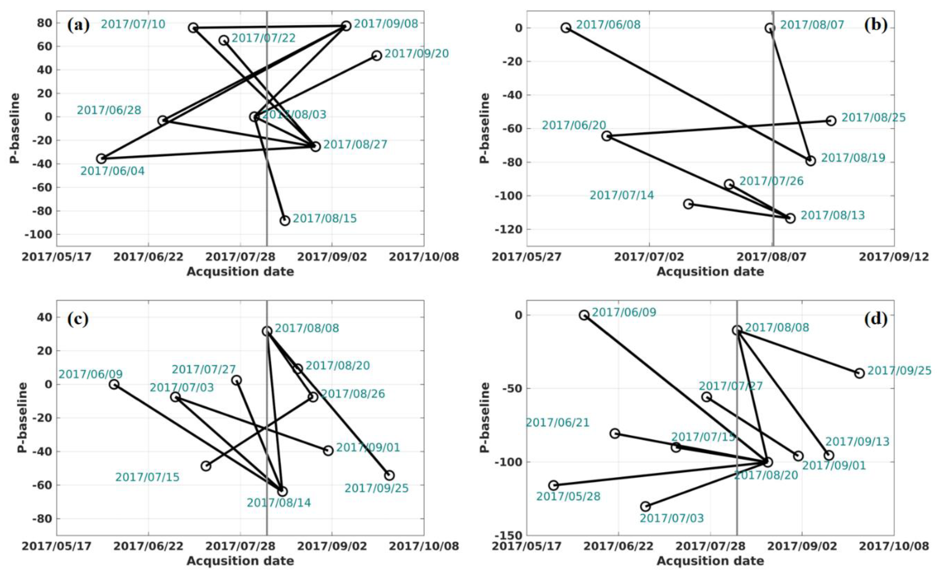
The 2017 Jinghe Mw 6.3 event was observed by four adjunct tracks, two in ascending orbit and two in descending orbit. From these, we generated interferometric displacement maps with four different viewing geometries. For each track, we created a stack of multi-temporal coseismic differential interferograms, and applied temporal averaging analysis to reconstruct the corresponding LoS coseismic displacement field. As mentioned above, we set perpendicular baseline () limits of ~100 m to reduce the impacts from the inaccuracies in the external terrain model. We limited the temporal baseline () to approximately four months (three months prior to and one month after the earthquake), in order to improve the coherence and reduce the post-seismic movement signals. The distributions of and for each S1 stack are shown in Figure 3. Through temporal averaging, the atmospheric turbulence is largely reduced, given that this component is considered to be a random signal in time.
All of the individual differential interferograms were processed using the GAMMA software. We processed the Sentinel-1 data with a multi-look factor of 10 in range and 2 in azimuth. The multi-looking step was employed to reduce the speckle noise while preserving a sufficient spatial resolution to reconstruct the coseismic deformation. Prior to the phase unwrapping, the generated interferograms were also filtered with an adaptive filter based on the local fringe spectrum [33]. A minimum cost flow (MCF) approach was applied to unwrap all of the generated interferograms [34,35].
Finally, we visually inspected the unwrapped interferograms, and those with severe atmospheric signals and unwrapping errors were discarded from the rest of the multi-temporal analysis step. During the selection, we also ensured that there were at least two interferograms connect to each SAR acquisition (Figure 3); this allowed for a level of redundancy that prevented residual errors (e.g., phase unwrapping errors) from propagating through the interferogram stack network [36]. Then, for the data from each single geometry, we applied temporal averaging to the selected unwrapped interferometric images. Finally, we generated four average coseismic displacement maps with different LoS viewing geometries; these were used for the slip distribution inversion.
3.3. ALOS2 PALSAR2 Interferogram Processing
We obtained three PALSAR2 images from the Japan Aerospace Exploration Agency (JAXA) archive (https://auig2.jaxa.jp/); these images were acquired on 13 March 2017, 14 August 2017, and 6 November 2017 (i.e., one before the earthquake and two after the earthquake). Two PALSAR2 pairs were processed following the same processing scheme applied to the individual S1 pair. The PALSAR2 stripmap Single Look Complex (SLC) pair was processed with a multi-look factor of three in range and four in azimuth. Note that the ionospheric distortions should have stronger impacts in the L-band PALSAR2 data than in the C-band Sentinel data, and are generally more significant at higher latitudes [37]. Nevertheless, the ionosphere signal is expected to be large in a spatial scale and mostly smooth in space [38]. Given that the Mw 6.3 Jinghe earthquake had a limited spatial extent, after masking the coseismic zone, we applied quadratic ramp modeling and removed this trend prior to displacement generation. We calculated the standard deviations (SD) of the derived interferometric displacement maps, which we used to indicate the level of existing artifacts. The pair of formed images acquired on 13 March 2017 and 6 November 2017 were selected, as they had the smallest standard deviation (SD; 2.44 cm); the pair formed by the images acquired on 13 March 2017 and 14 August 2017 had an SD of 2.97 cm. The of the selected pair was 91 m, satisfying the criteria (see Section 3.1). Overall, using this data processing scheme, we minimized the contribution of nuisance signals and generated LoS coseismic deformation with a single PALSAR2 pair.
3.4. Displacement Fields Analysis and Evaluation
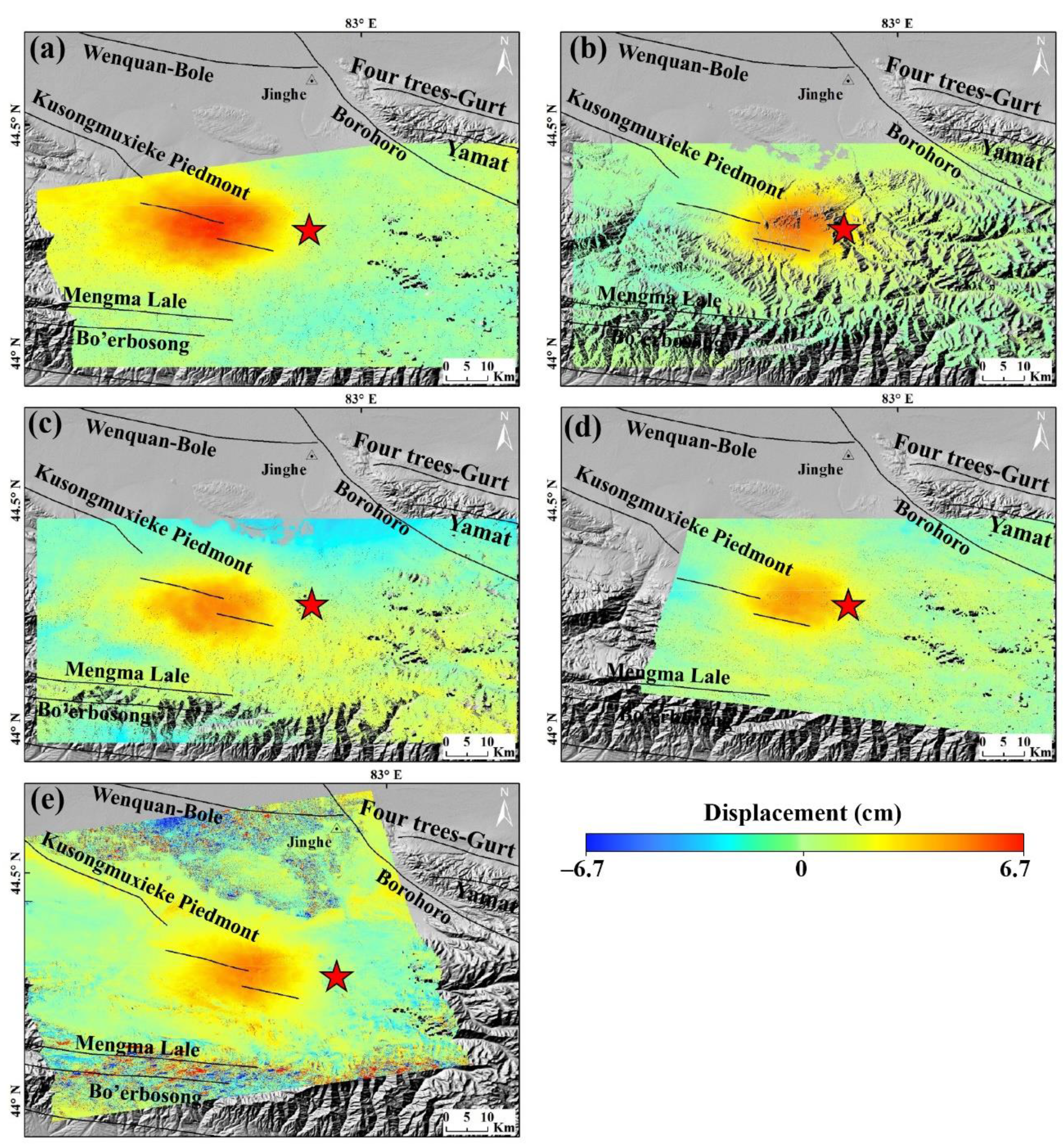
We obtained five multi-geometric coseismic displacement maps for the Jinghe 2017 event, four from S1 and the other one from ALOS2 PALSAR2 (Figure 4). The maps show that the coseismic displacement formed an ellipse-like shape. Theoretically, the displacement fields caused by thrust faulting consist of two sub-fields moving in opposite directions [39]. However, in the case of Jinghe, we could not delineate the movements caused by the footwall. This single side movement pattern is very common in InSAR studies of moderate thrusts (e.g., the Hutubi Earthquake [10] and Menyuan Earthquake [40]). The PALSAR2 interferogram (Figure 4e) contained a significant decorrelated zone in the mountain region south of the epicenter, and another in a nearby farming area of Jinghe County. Note that the ALOS2 PALSAR2 pair had a larger temporal baseline (238 days), and thus a significant ground coverage change within this period was expected. The decorrelation is observed in Figure 4e, including in a farming area northeast of KPF and a mountainous area to the south of Mengma Lale fault. The InSAR observed signals in these areas are likely associated with decorrelation artifacts and unwrapping errors.
Table 2 shows the standard deviation (SD) of the temporally averaged S1 interferometric pairs and of the selected ALOS2 interferogram, along with the view geometry parameters and detected maximum displacement. As an indication of the noise level, the SD decreased after applying temporal averaging. Furthermore, the overall noise level in the descending tracks was smaller than that in the ascending tracks. The incidence angles of the two adjunct tracks differed by ~10°, and this is the main reason for the large differences in the detected maximum LoS displacements of the different tracks. The S1 T12 ascending result has a similar viewing geometry to the ALOS2 PALSAR2 result, and both show a maximum displacement of ~6 cm. Furthermore, the ascending pairs (e.g., S1-T12 and ALOS2) captured more displacement signals than those from the descending pair (S1-T63), despite the incidence angles being similar. This indicates that the geometric differences carry information that is useful for constraining the attributes of the seismogenic fault.
However, the geometric differences between these five displacement maps were not sufficient for us to apply a 3D deformation decomposition, because they all were observed by right-looking satellites; as such, there was a strong correlation between each viewing geometry. The remaining NS displacement uncertainty should be very large [41]. Therefore, we applied a joint inversion of all five displacement results to quantify the attributes of the seismogenic fault of the 2017 Jinghe event.
4. Fault Parameters and Slip Distribution Inversion
The inversion of seismic source mechanisms based on geodetic measurements is an important tool for understanding seismogenic structures and for evaluating future regional earthquake risk. We modeled the source parameters by elastic dislocation modeling using the interferometric displacement results shown in Section 3.4. First, we determined the fault strike based on the focal mechanism solutions and regional geological information. Next, we employed a package developed by Wang et al. [42] of the German Research Centre for Geosciences (GFZ), which achieves constrained least-squares optimization by employing the Steepest Decent Method (SDM) in order to conduct geodetic inversion.
The spatial extension of the deformation field produced by the earthquake was ~18 km N–S and ~21 km E–W. Prior to the modeling processes, we cropped out the main deformation area from the overall InSAR coverage. In this way, we avoided most of the decorrelation zones to the southwest (i.e., those associated with the Tian Shan Mountains) and to the northeast (i.e., those associated with the Jinghe Country farming area). For the LoS displacement maps of each viewing geometry, several hundred thousand pixels remained. To further reduce the data size, we applied quadtree decomposition (e.g., Jónsson et al. [43]) to each displacement map. Quadtree down-sampling retains important information (e.g., the deformation field gradient), but reduces noise contributions and improves computational efficiency. Finally, the sample pixels were reduced from millions to a few thousand.
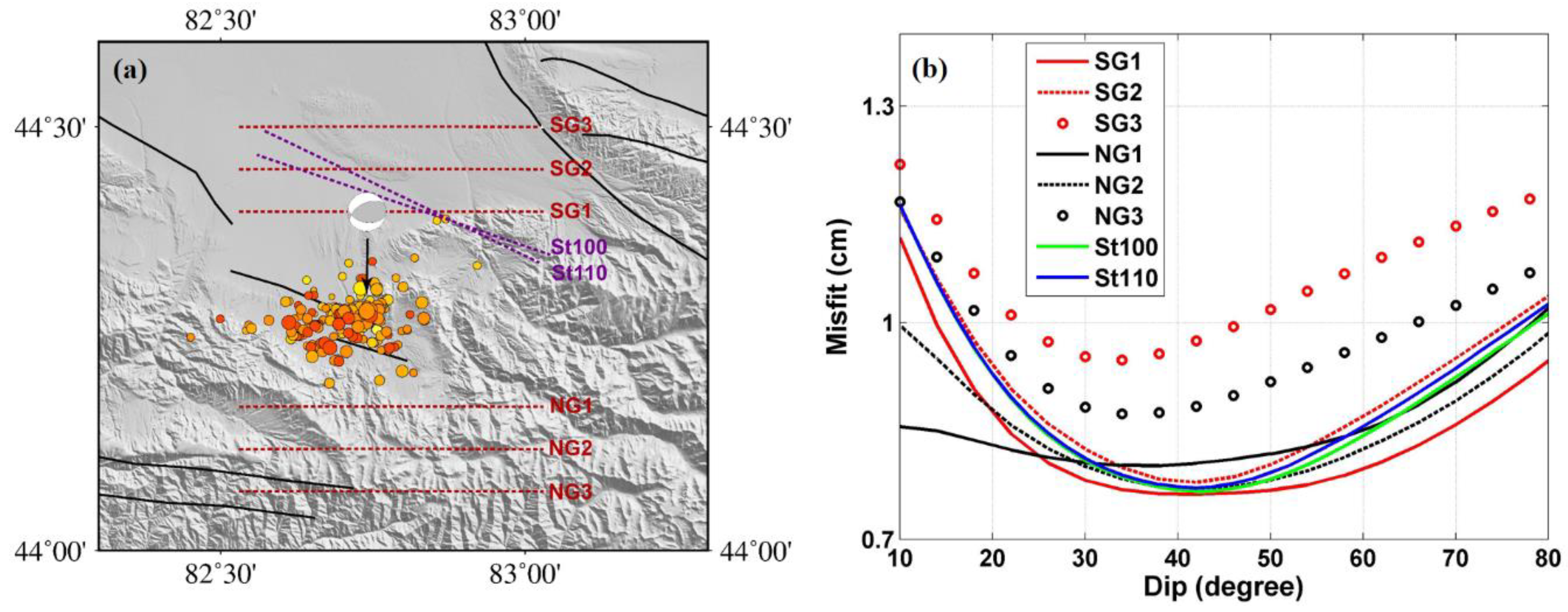
The determination of the fault geometry model is another key step in the slip distribution inversion. Given that the rupture of the Jinghe 2017 earthquake had no surface expression, it is difficult to determine the fault geometry without prior knowledge. First, we examined the fault geometry based on data from regional geology and focal mechanism solutions. As shown in Figure 1, major faults (e.g., KPF and MLF) in the Jinghe area extend approximately WNW–ESE along the northern Tian Shan Mountains. The focal mechanism solutions published by multiple facilities (Table 1) suggest that the seismogenic fault strikes in E–W (USGS solution) or WNW–ESE (GCMT solution); moreover, the dipping direction remains a subject of debate. Previous studies [11,12,13] on the Jinghe Mw6.3 earthquake all suggest that the seismogenic fault is approximately south dipping; however, based on evidence from studies of other earthquakes under similar tectonic backgrounds, the north dipping back-thrust could also represent the seismogenic fault. For example, using the InSAR and relocated aftershock data, Wang et al. [10] suggested that the 2016 Mw 6.0 Hutubi earthquake, which occurred within a similar geological setting in the northern Tian Shan region, could have occurred on a back-thrust associated with the Huoerguosi–Manas–Tugulu fault. Therefore, we built two groups of candidate fault models in an EW direction on the side of the displacement field, including a south-dipping group and a north-dipping group, with the purpose of searching for the optimal fault location (Figure 5a).
Each group contains three candidate fault models sharing the same strike direction, dimension, and a similar dipping orientation. The distance between each neighborhood candidate fault is 5 km. All of these candidate fault models are single-segment models in an elastic half-space [44]. As shown in Figure 5a, the ground traces of NG1 and SG1 lie approximately 14 km away from the epicenter. All of the candidate faults have dimensions of ~50 km along-strike, and 60 km in the down-dip direction. For each candidate model, we discretized the fault plane into 2 × 2 km fault patches, and solved for the fault slip on each patch using the elastic half-space dislocation model and a Poisson ratio of 0.25. The corresponding dip angle was determined through trials by minimizing the misfit, with its initial value range varying between 10° and 80°. The model misfit in the form of the root-mean-square-error (RMSE) was calculated for each inversion result. As the five InSAR displacement maps had different seed points causing unknown constant offsets, we also included an offset parameter in the geodetic inversion. Figure 5b display the relationship misfit vs. dip for each of the candidate fault models. Among the models, the south dipping model, SG1, produces the minimum misfit. The north dipping model, NG2, behaves better than the other two north dipping models. The optimal dip angle for both SG1 and NG2 is 42°.
Therefore, we picked the north dipping model, NG2. centered at 44.12°N and 82.84°E, striking N270E°, and the south dipping model, SG1, centered at 44.4°N and 82.84°E, striking N90°E, to further discuss the optimal dip direction. Next, we fixed the fault strike, length, bottom depths, and optimal dip determined through the aforementioned trails, and allowed the rake and the amount of slip to vary in the inversion.
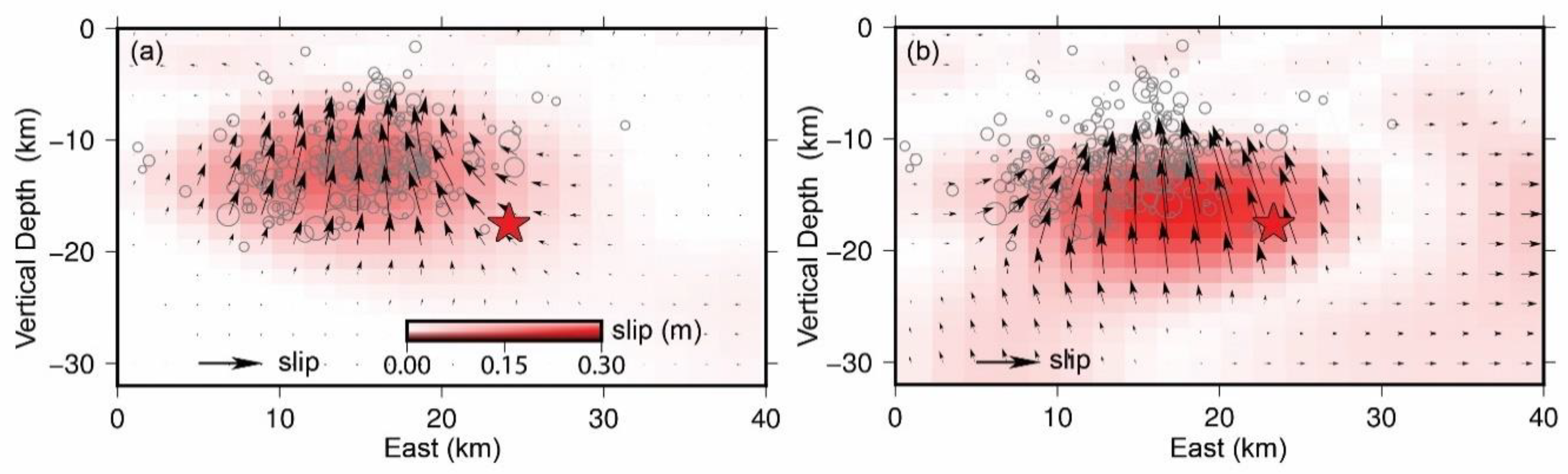
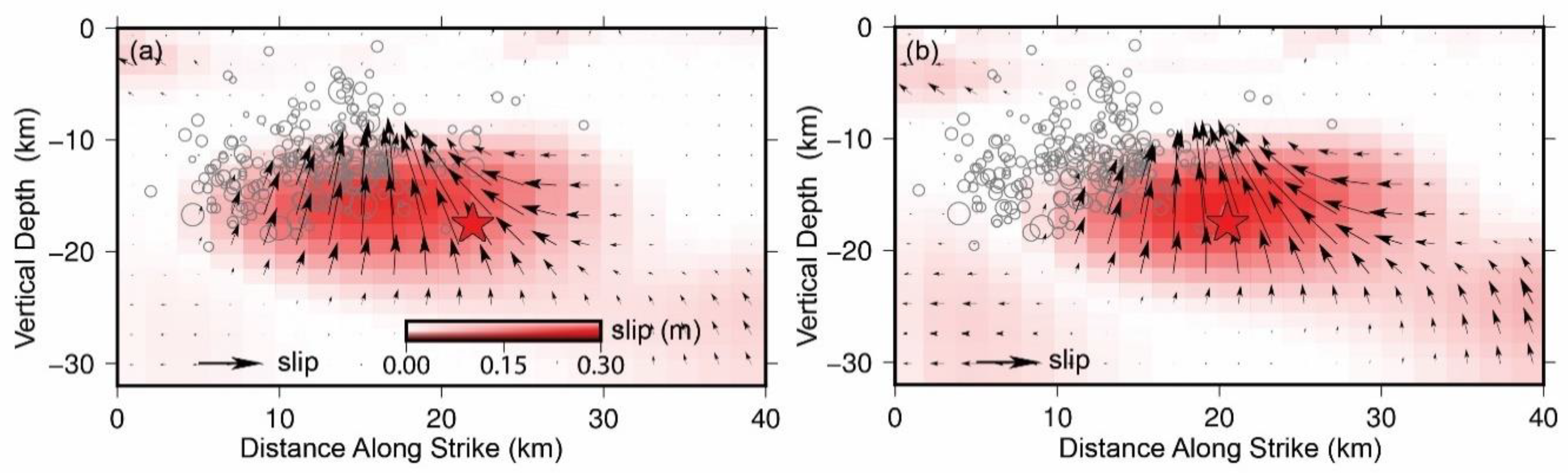
The inverted parameters of the two fault models are shown in Table 3. Figure 6 shows the slip distribution of each fault model in a vertical cross section. For the north dipping model, most of the slip was in a region with a vertical depth of 10–25 km. The maximum slip (0.37 m) occurred at 16.73 km, with a rake angle of 84.02°. The estimated geodetic moment was 4.52 × 10¹⁸ N m, corresponding to a Mw 6.37 event. For the southing dipping model, the main slip zoom was distributed between 5 and 20 km in vertical depth. The maximum slip (0.25 m) occurred at 14.05 km, and the associated rake was 89.56°. The estimated geodetic moment was 2.42 × 10¹⁸, corresponding to a Mw 6.19 event.
As shown in Figure 6, our best-fitting solution revealed a simple slip distribution in both the north- and south-dipping models. In the same figure, we added the location of the relocated Jinghe earthquake sequence derived by Liu et al. [12], for display and analysis. This sequence covers a time span between 8 August and 30 September 2017. Here, the displacement derived by InSAR represents the cumulative displacement that occurred between May and September 2017, under the assumption that coseismic deformation dominates the signal; as such, this slip distribution cannot distinguish between the mainshock and the events that occurred within the following 2 months. Nevertheless, the result derived from the south dipping fault is generally consistent with the distributions of the published sequence relocations, and the associated model misfit is also comparably smaller; in contrast, the results from the north dipping fault model are deeper; therefore, between the two, we prefer the south dipping fault model.
Next, we further considered the strike direction for the purpose of optimizing the above-selected south dipping fault model. We built two extra candidate fault models with different strike directions, one at 100° and one at 110°. These two faults lie in the area around the previously tested SG1 and SG2. Their locations are shown in Figure 5a (as St100 and St110 for a strike of 100° and 110°, respectively). We carried out the dip angle optimization through a grid search, and selected the one that minimized the misfit. The optimal dip angle of fault models St100 and St110 was found to be 42°. The misfit vs. dip curves of these two models are displayed in Figure 5b, which shows a similar capability in minimizing the inversion misfit. Then, the same inversion step was applied to both models in order to quantify the associated slip distributions; the result is shown in Figure 7.
For both models, the main slip zone is within a vertical depth of 10–25 km, slightly deeper than the EW striking south dipping model. For St100, the maximum slip (0.34 m) occurred at approximately 16.7 km with a rake angle of 96.77°; for St110, the maximum slip (0.36 m) also occurred at approximately 16.7 km with a rake angle of 107.98°. By rotating the faults from EW to WNW–ESE, the maximum slip and associated rake angle and depth were increased. However, the discrepancy between the main slip zone and the relocated earthquake sequence also increased (Figure 7). Therefore, we do not believe that WNW–ESE striking models can better describe the fault geometry of the 2017 Jinghe event. However, this could also because our derived InSAR results do not have sufficient resolution to distinguish among strike angles of 90° to 110°.
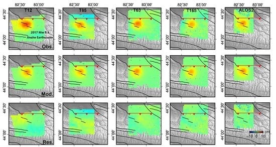
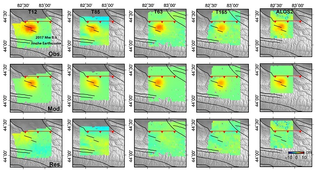
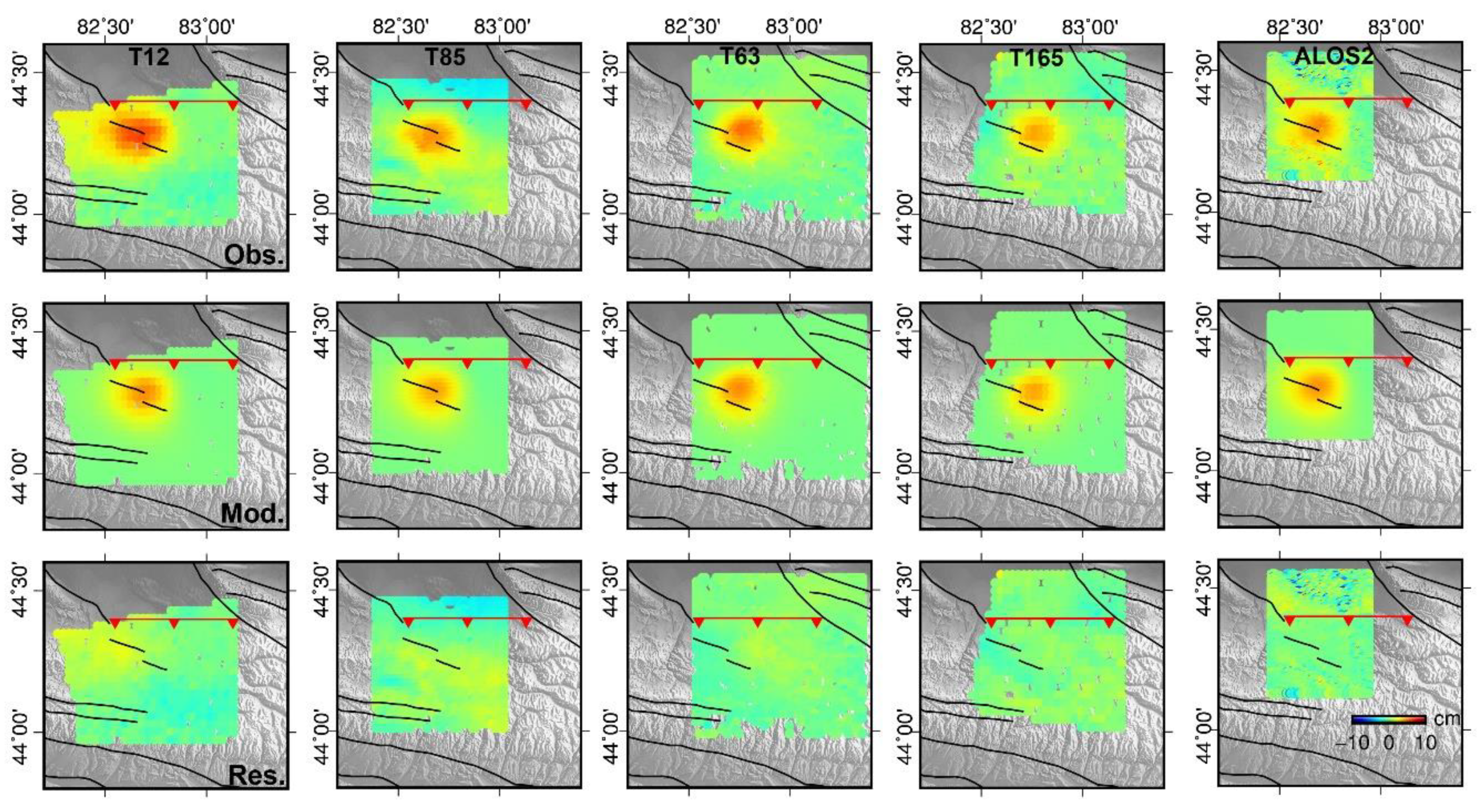
Overall, the best-fitting result inverted from multi-geometry InSAR inputs favors the south dipping model striking in an EW direction. As shown in Figure 8, the misfits (RMS) for both fault models were generally less than 1 cm, the only exception being for the ALOS2 data, for which the data points show higher residuals. This larger misfit for ALOS2 data is mainly caused by the interferometric decorrelation in the farming area, which is away from the coseismic deformation zone. Otherwise, there is no significant deviation between the InSAR observations and modeled deformation.
5. Discussion
The use of multi-temporal and multi-geometry InSAR data reduced the noise level of the reconstructed coseismic deformation maps (Table 2). However, for the moderate earthquakes, challenges remain when using geodetic observations alone to infer the fault dip orientation [45,46]. Such an analysis requires additional geological or geophysical constraints. With the relocated earthquake sequence derived by Liu et al. [12], we believe that the south dipping model with a strike of 90° better describes the fault geometry of the 2017 Jinghe event. Because it is generally more consistent with the vertical distributions of the published earthquake sequence relocations, compared with the other candidate models.
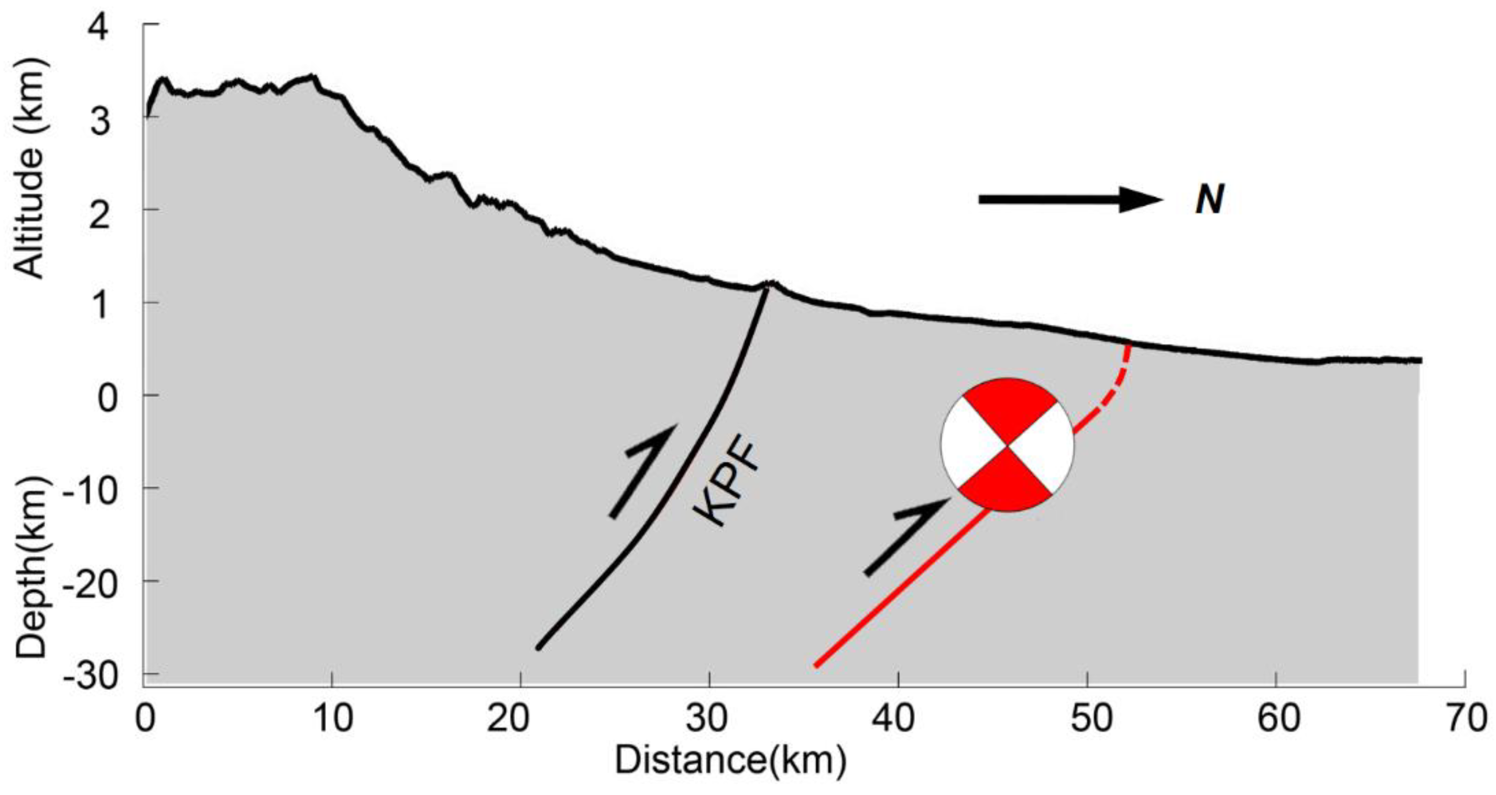
This determined seismogenic fault has not yet been mapped, and we suspect it is a blind fault striking ~N90°E, centered at ~44.4° and 82.84°E, and dipping towards the south at an angle of ~42°. Figure 9 is a sketch map demonstrating the relative location of the derived fault and KPF. The fault is approximately 15 km north of the KPF. Note that the KPF is also a south dipping reverse fault, with a dip angle between 40° and 60° [20]. Note that SG1 lies in the front of a small hill north of the epicenter (see Figure 5a), and the striking direction of SG1 is approximately parallel to this hill. Considering the relative locations of the suggested blind fault and the KPF, this blind fault could be formed by the northward propagation of KPT. With the continuing NS shortening of the Tian Shan Mountain Range, fold-thrust belts to the south and north of the mountain front will propagate into the foreland [8,19]. The 2017 Mw 6.3 Jinghe earthquake could represent a relief response to the strain accumulated by this NS shortening. However, given the limited capability of InSAR, in the constrained dip and also strike as tested above, we suggest that a comprehensive geological investigation of this region is needed in order to confirm the characteristics of the seismogenic fault.
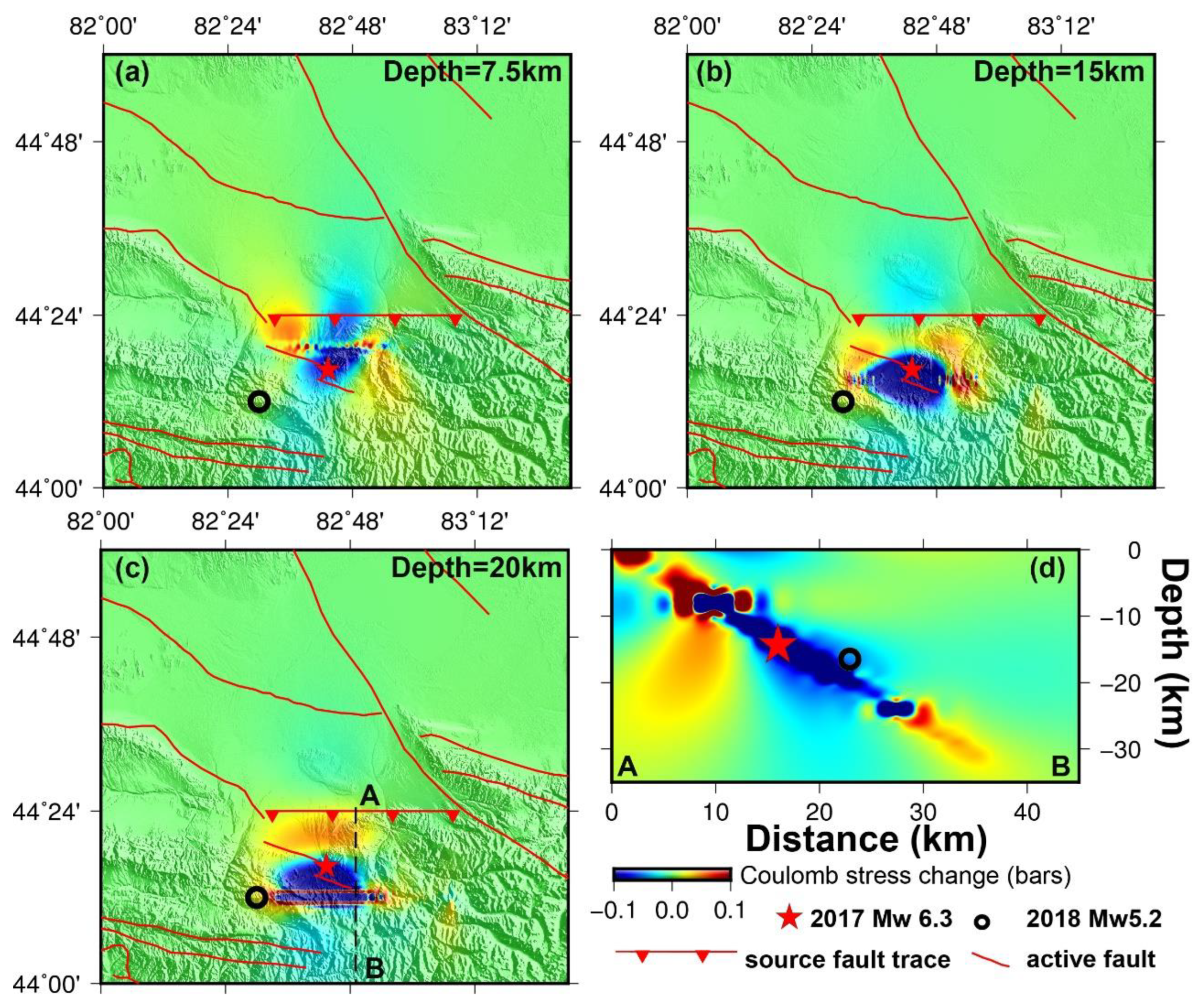
We calculated the static Coulomb stress change induced by the 2017 Mw 6.3 event in order to discuss its relationship to the 2018 Mw 5.2 Jinghe earthquake. In 2018, another Mw 5.2 reverse faulting earthquake hit Jinghe County [22]. The relocated epicenter was at 82.5°E–44.20°N, and it had a focal depth of ~16 km [23]. The epicenter is away from the stress increase zone caused by the 2017 Mw 6.3 event. Figure 10d shows a cross-section of the coseismic Coulomb stress change along profile A–B (Figure 10c), and highlights the relative geometry between the suggested blind fault and the epicenter of the 2018 Mw 5.2 event. Based on the relative location of the 2018 event and the distribution of the Coulomb stress change, it is not likely that the 2017 and 2018 events were triggered by the same blind thrust fault.
Figure 10b also indicates an increased Coulomb stress change at shallower depths (~0–10 km) of the suggested blind fault. This is because the 2017 Jinghe event did not rupture to the surface; as such, the possibility remains for either a rupture or aseismic slip of the upper part of this fault, depending on the frictional properties of the fault plane and the regional stress state. Based on the fault trace determined in this study (Figure 8b), a rupture at the surface would be likely to occur closer to the town of Jinghe, where most of the region’s population and infrastructure are located. To better assess the future seismic hazard, it is necessary estimate the equivalent aseismic-moment caused by postseismic deformation, and to evaluate the overall slip deficit budget [47,48]. Therefore, we suggest that a more detailed geological study is needed, along with the continuous geodetic monitoring of this region.
6. Conclusions
In this study, we used multi-source and multi-track satellite SAR imagery to reconstruct the coseismic displacement field of the 2017 Mw 6.3 Jinghe earthquake. We employed the multi-temporal scenes acquired by Sentinel-1, and reconstructed the coseismic deformation signal through a temporal averaging strategy in order to reduce the phase artifacts. Together with a single-pair result derived from the ALOS2 data, we obtained five displacement maps with slightly different viewing geometries. All of these were used to constrain the geodetic inversion in order retrieve the fault geometry parameters and slip distribution. For future earthquake applications if the same temporal averaging strategy applied, one should keep the time period after the main shock as short as possible in order to reduce the impact from the postseismic displacement.
Based on the focal mechanism and regional geological information and the regional geological structure, we built multiple fault models with different dipping directions (south and north dipping) and various striking directions (striking of 90°, 100°, and 11°). The south dipping model in the EW strike is preferred, because its associated slip depth is more consistent with the relocated earthquake sequence [12]. This south dipping model indicates a blind thrust fault located north of the KPF into the foreland; the corresponding optimal dip angle is ~42°. This source model generates a geodetic moment of 2.42 × 10¹⁸, corresponding to a Mw 6.19 event. A significant slip is located between vertical depths of 5 and 20 km. Given the regional geology, we speculate that this blind fault could be formed by the northward propagation of the KPT, owing to the continuous NS shortening of the Tian Shan Mountains. Given that the upper part of the determined blind fault did not rupture during the 2017 event, the likelihood of future earthquakes in this region remains high. We suggest that a thorough geological survey of this region is needed in order to further investigate the existence of this blind fault; this should be accompanied by the continuous monitoring of postseismic deformation in order to better evaluate the seismic risk in Jinghe County.
Author Contributions
conceptualization, W.G. and X.S.; methodology, W.G.; software, W.G.; validation, W.G., Y.Z., T.L., and S.W.; formal analysis, W.G. and Y.Z.; investigation, W.G. and Y.Z.; resources, W.G.; data curation, W.G.; writing—original draft preparation, W.G.; writing—review and editing, W.G., D.Z., and T.L.; visualization, W.G. and Y.Z.; supervision, X.S.; project administration, W.G. and L.H.; funding acquisition, W.G.
Funding
This research was funded by the National Natural Science Foundation of China, grant number 41604008.
Acknowledgments
We would like to thank all of the anonymous reviewers for their insightful comments on the paper. The Sentinel-1 data is provided by European Space Agency (ESA), through the Alaska Satellite Facility (vertex.daac.asf.alaska.edu). The ALOS2 PALSAR2 data is provided by the Japan Aerospace Exploration Agency (JAXA), through the research proposal (ID: P1214002). We would like to express great thanks to Jianming Liu from the Earthquake Administration of Xinjiang Province China for sharing the earthquake sequence relocation data. We thank Mingsheng Liao and Heng Luo from Wuhan University for their valuable remarks in data processing. We thank Kaihua Ding from the China University of Geosciences, and Wuhan and Jianjun Wang from Wuhan University for their helpful discussion. We also thank Sarah Henton De Angelis from Tornillo Scientific for her great comments.
Conflicts of Interest
The authors declare no conflict of interest.
References
- CENC. 2017/08/09 Jinghe, Xinjiang Province M6.6 Earthquake. Available online: https://www.cenc.ac.cn/cenc/_300651/335684/index.html (accessed on 1 February 2019).
- USGS. M 6.3—109km SSE of Dostyq, Kazakhstan. Available online: https://earthquake.usgs.gov/earthquakes/eventpage/us2000a65e/executive (accessed on 1 February 2019).
- Ekström, G.; Nettles, M.; Dziewonski, A. The global CMT project 2004–2010: Centroid-moment tensors for 13,017 earthquakes. Phys. Earth Planet. Inter. 2012, 200, 1–9. [Google Scholar] [CrossRef]
- Dziewonski, A.M.; Chou, T.-A.; Woodhouse, J.H. Determination of earthquake source parameters from waveform data for studies of global and regional seismicity. J. Geophys. Res. Space Phys. 1981, 86, 2825–2852. [Google Scholar] [CrossRef]
- Jiang, X.; Han, Y.; Yang, W.; Meng, L. Preliminary analysis of the 2017 Jinghe Ms 6.6 earthquake sequence and its seismic source characteristics. Earthq. Res. China 2017, 33, 682–693. [Google Scholar]
- Ghose, S.; Hamburger, M.W.; Ammon, C.J. Source parameters of moderate-sized earthquakes in the Tien Shan, central Asia from regional moment tensor inversion. Geophys. Res. Lett. 1998, 25, 3181–3184. [Google Scholar] [CrossRef]
- Avouac, J.P.; Tapponnier, P.; Bai, M.; You, H.; Wang, G. Active thrusting and folding along the northern Tien Shan and Late Cenozoic rotation of the Tarim relative to Dzungaria and Kazakhstan. J. Geophys. Res. Space Phys. 1993, 98, 6755–6804. [Google Scholar] [CrossRef] [Green Version]
- Deng, Q.; Feng, X.; Yang, X. Study on Holocene paleoearthquake by large trench in the Manas-Tugulu reverse faultand-fold zone along Northern margin of the Tian Shan mountain in Xinjiang. In Research on Active Faults Series; Seismological Press: Beijing, China, 1994; Volume 3. (In Chinese) [Google Scholar]
- Qiao, X.; Wang, Q.; Yang, S. Study on the focal mechanism and deformation characteristics for the 2008 Mw6.7 Wuqia earthquake, Xinjiang by InSAR. Chin. J. Geophys. 2013, 57, 1805–1813. (In Chinese) [Google Scholar]
- Wang, X.; Xu, C.; Wen, Y.; Wang, S.; Xu, G.; Xiao, Z.; Fang, L. The 2016 Mw 6.0 Hutubi earthquake: A blind thrust event along the northern Tian Shan front. J. Asian Earth Sci. 2019, 173, 79–87. [Google Scholar] [CrossRef]
- Bai, L.; Liu, J.; Zhang, Y.; Wu, Q.; An, Y. Relocation of the 2017 Ms 6.6 Jinghe, Xinjiang earthquake sequence and its seismogenic structure. Earthq. Res. China 2017, 33, 703–711. [Google Scholar]
- Liu, J.; Gao, R.; Wang, Q.; Nie, X. Relocation of the Jinghe Ms 6.6 earthquake sequence on August 9, 2017 and analysis of the seismogenic structure. Earthq. Res. China 2017, 33, 663–670. (In Chinese) [Google Scholar]
- Liu, C.; Qiu, J.; Wang, J. The 2017 Jinghe Ms 6.6 Earthquake Inversion from Ascending and Descending Sentinel-1 Observations. J. Geod. Geodyn. 2018, 38, 1111–1116. [Google Scholar]
- Kreemer, C.; Blewitt, G.; Klein, E.C. A geodetic plate motion and Global Strain Rate Model. Geochem. Geophys. Geosyst. 2014, 15, 3849–3889. [Google Scholar] [CrossRef]
- Burchfiel, B.C.; Brown, E.T.; Qidong, D.; Xianyue, F.; Jun, L.; Molnar, P.; Jianbang, S.; Zhangming, W.; Huichuan, Y. Crustal Shortening on the Margins of the Tien Shan, Xinjiang, China. Int. Geol. Rev. 1999, 41, 665–700. [Google Scholar] [CrossRef]
- Yang, S.; Li, J.; Wang, Q. The deformation pattern and fault rate in the Tianshan Mountains inferred from GPS observations. Sci. China Ser. D Earth Sci. 2008, 51, 1064–1080. [Google Scholar] [CrossRef]
- Tapponnier, P.; Molnar, P. Active faulting and cenozoic tectonics of the Tien Shan, Mongolia, and Baykal Regions. J. Geophys. Res. Space Phys. 1979, 84, 3425–3459. [Google Scholar] [CrossRef]
- Weldon, R.J.; Rubin, C.M.; Molnar, P.; Thompson, S.C.; Abdrakhmatov, K.; Berger, G.W. Late Quaternary slip rates across the central Tien Shan, Kyrgyzstan, central Asia. J. Geophys. Res. Space Phys. 2002, 107, 1–32. [Google Scholar]
- Deng, Q.; Feng, X.; Zhang, P.; Xu, X.; Yang, X.; Peng, S.; Li, J. Active Tectonic of Tian Shan, 1st ed.; Seismological Press: Beijing, China, 2000. (In Chinese) [Google Scholar]
- Chen, J.; Shen, J.; Li, J.; Yang, J.; Hu, W.; Zhao, X.; Zeng, X. Preliminary study on new active characteristics of Kusongmuxieke mountain front fault in the west segment of north Tianshan. Northwest. Seismol. J. 2007, 29, 335–340. (In Chinese) [Google Scholar]
- Chen, J.; Tan, M.; Wu, G.; Hu, W.; Sun, J.; Zhang, Z. The Seismic Damage Characteristic and the Cause of the Jinhe M5.0 Earthquake in Xinjiang on Oct. 16, 2011. Technol. Earthq. Disaster Prev. 2012, 7, 164–172. (In Chinese) [Google Scholar]
- USGS. M 5.2—112km ENE of Yining Xian, China. Available online: https://earthquake.usgs.gov/earthquakes/eventpage/us1000hcmu/moment-tensor (accessed on 1 February 2019).
- Liu, P.; Han, G.; Nie, X. M5.4 Earthquake on October 16, 2018 in Jinghe Xinjiang; Earthquake Administration of Xinjiang, CEA: Beijing, China, 2018. [Google Scholar]
- ASF. Sentinel-1. Available online: https://www.asf.alaska.edu/sentinel/ (accessed on 1 February 2019).
- Parsons, B.; Wright, T.; Fielding, E. Measurement of interseismic strain accumulation across the North Anatolian Fault by satellite radar interferometry. Geophys. Res. Lett. 2001, 28, 2117–2120. [Google Scholar]
- JAXA. ALOS-2 Basic Observation Scenario, 1st ed.; JAXA: Tokyo, Japan, 2014. Available online: http://www.eorc.jaxa.jp/ALOS-2/en/obs/scenario/ALOS-2_Basic_Observation_Scenario_First-Ed_E_v00.pdf (accessed on 1 February 2019).
- Hanssen, R. Radar Interferometry: Data Interpretation and Error Analysis, 1 ed.; Kluwer Academic Publishers: Amsterdam, The Netherlands, 2001; Volume 2. [Google Scholar]
- Zebker, H.A.; Rosen, P.A.; Hensley, S. Atmospheric effects in interferometric synthetic aperture radar surface deformation and topographic maps. J. Geophys. Res. Space Phys. 1997, 102, 7547–7563. [Google Scholar] [CrossRef]
- Gonzalez, P.J.; Tiampo, K.F.; Camacho, A.G.; Fernández, J. Shallow flank deformation at Cumbre Vieja volcano (Canary Islands): Implications on the stability of steep-sided volcano flanks at oceanic islands. Earth Planet. Sci. Lett. 2010, 297, 545–557. [Google Scholar] [CrossRef]
- Jiang, L.; Li, C.; Qiu, G.; Wang, H.; Wright, T.J.; Yu, Y.; Lin, H. InSAR reveals coastal subsidence in the Pearl River Delta, China. Geophys. J. Int. 2012, 191, 1119–1128. [Google Scholar] [Green Version]
- Dong, J.; Zhang, L.; Liao, M.; Gong, J. Improved Correction of Seasonal Tropospheric Delay in InSAR Observations for Landslide Deformation Monitoring. Remote Sens. Environ. 2019. under review. [Google Scholar] [CrossRef]
- Bie, L.; Ryder, I.; Nippress, S.E.; Bürgmann, R. Coseismic and post-seismic activity associated with the 2008 Mw 6.3 Damxung earthquake, Tibet, constrained by InSAR. Geophys. J. Int. 2013, 196, 788–803. [Google Scholar] [CrossRef]
- Goldstein, R.M.; Werner, C.L. Radar interferogram filtering for geophysical applications. Geophys. Res. Lett. 1998, 25, 4035–4038. [Google Scholar] [CrossRef] [Green Version]
- Werner, C.L.; Wegmüller, U.; Strozzi, T. Processing Strategies for Phase Unwrapping for InSAR Applications. In Proceedings of the EUSAR 2002—4th European Conference on Synthetic Aperture Radar, Cologne, Germany, 4–6 June 2002; pp. 353–356. [Google Scholar]
- Costantini, M. A novel phase unwrapping method based on network programming. IEEE Trans. Geosci. Remote Sens. 1998, 36, 813–821. [Google Scholar] [CrossRef]
- Doin, M.P.; Guillaso, S.; Jolivet, R.; Lasserre, C.; Lodge, F.; Ducret, G.; Gradin, R. Presentation of the small baseline NSBAS processing chain on a case example: The Etna deformation monitoring from 2003 to 2010 using Envisat data. In Proceedings of the ESA FRINGE 2011 Conference, Frascati, Italy, 19–23 September 2011. [Google Scholar]
- Gray, A.L.; Mattar, K.E. Influence of Ionospheric Electron Density Fluctuations on Satellite Radar Interferometry. Geophys. Res. Lett. 2000, 27, 1451–1454. [Google Scholar] [CrossRef]
- Meyer, F. A review of ionospheric effects in low-frequency SAR—Signals, correction methods, and performance requirements. In Proceedings of the 2010 IEEE International Geoscience and Remote Sensing Symposium (IGARSS), Honolulu, HI, USA, 25–30 July 2010; pp. 29–32. [Google Scholar]
- King, G.C.P.; Stein, R.S.; Rundle, J.B. The Growth of Geological Structures by Repeated Earthquakes 1. Conceptual Framework. J. Geophys. Res. Space Phys. 1988, 93, 13307–13318. [Google Scholar] [CrossRef]
- Liu, Y.; Zhang, G.; Zhang, Y.; Shan, X. Source parameters of the 2016 Menyuan earthquake in the northeastern Tibetan Plateau determined from regional seismic waveforms and InSAR measurements. J. Asian Earth Sci. 2018, 158, 103–111. [Google Scholar] [CrossRef]
- Parsons, B.E.; Lu, Z.; Wright, T.J. Toward mapping surface deformation in three dimensions using InSAR. Geophys. Res. Lett. 2004, 31. [Google Scholar] [CrossRef] [Green Version]
- Wang, R.; Diao, F.; Hoechner, A. SDM—A geodetic inversion code incorporating with layered crust structure and curved fault geometry. In Proceedings of the General Assembly European Geosciences Union, Vienna, Austria, 7–12 April 2013. [Google Scholar]
- Jonsson, S. Fault Slip Distribution of the 1999 Mw 7.1 Hector Mine, California, Earthquake, Estimated from Satellite Radar and GPS Measurements. Bull. Seism. Soc. Am. 2002, 92, 1377–1389. [Google Scholar] [CrossRef]
- Okada, Y. Surface Deformation Due to Shear and Tensile Faults in a Half-Space. Seismol. Soc. Am. 1985, 75, 1135–1154. [Google Scholar]
- Lohman, R.; Barnhart, W.D. Evaluation of earthquake triggering during the 2005–2008 earthquake sequence on Qeshm Island, Iran. J. Geophys. Res. Space Phys. 2010, 115. [Google Scholar] [CrossRef]
- Lohman, R.B.; Simons, M.; Savage, B. Location and mechanism of the Little Skull Mountain earthquake as constrained by satellite radar interferometry and seismic waveform modeling. J. Geophys. Res. Space Phys. 2002, 107, 7–10. [Google Scholar] [CrossRef]
- Mencin, D.; Bendick, R.; Upreti, B.N.; Adhikari, D.P.; Gajurel, A.P.; Bhattarai, R.R.; Shrestha, H.R.; Bhattarai, T.N.; Manandhar, N.; Galetzka, J.; et al. Himalayan strain reservoir inferred from limited afterslip following the Gorkha earthquake. Nat. Geosci. 2016, 9, 533–537. [Google Scholar] [CrossRef]
- Wimpenny, S.; Copley, A.; Ingleby, T. Fault mechanics and post-seismic deformation at Bam, SE Iran. Geophys. J. Int. 2017, 209, 1018–1035. [Google Scholar] [CrossRef] [Green Version]
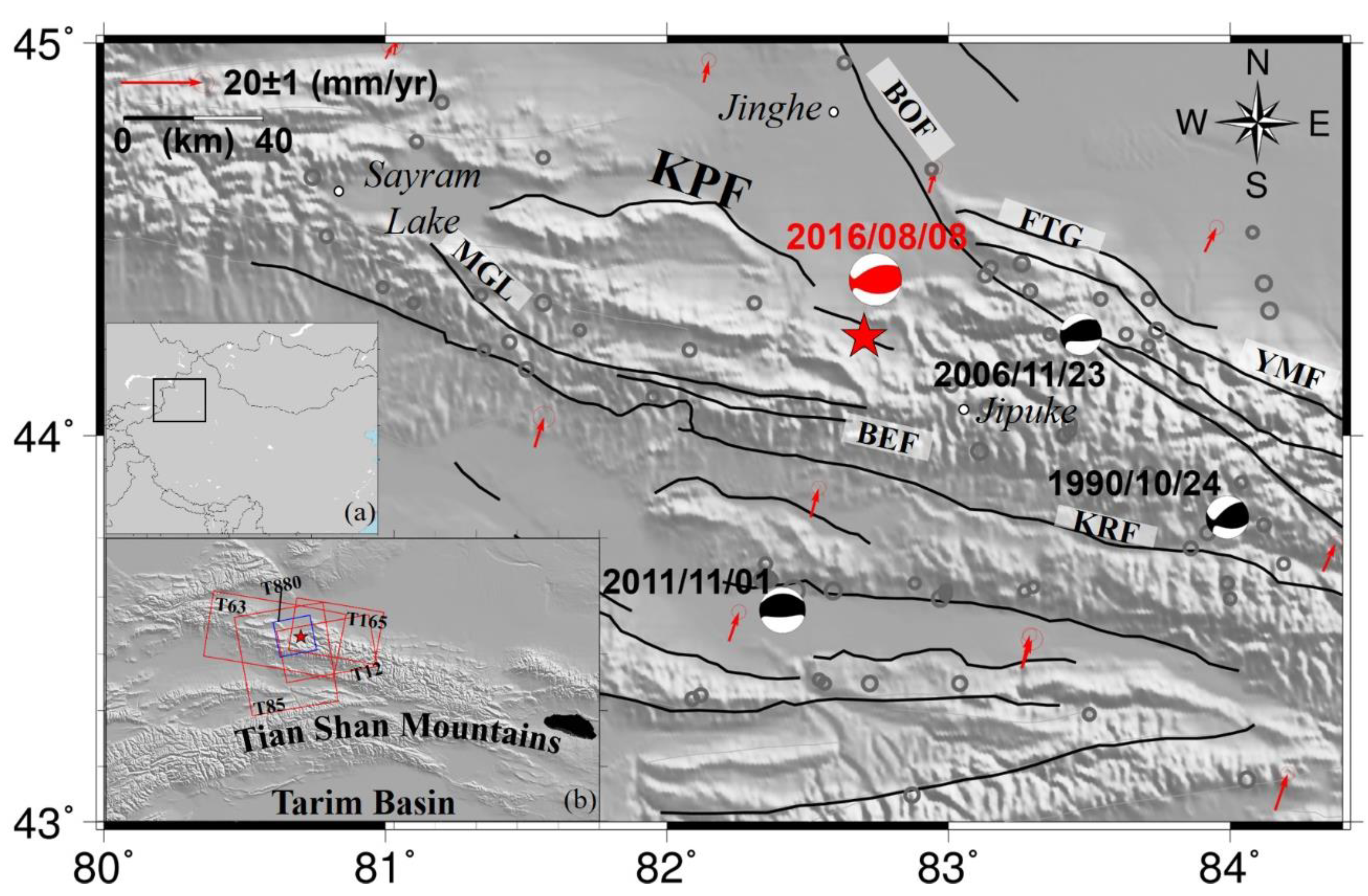
Figure 1.
Tectonic setting of the study area with focal mechanism solutions of Mw >5 earthquakes derived from the Global Centroid Moment Tensor GCMT ([3]; red for the 2017 Mw 6.3 Jinghe earthquake, black for historical events). The red star denotes the epicenter of the Mw 6.3 Jinghe earthquake. Gray circles denote instrumental earthquakes (Mw >3) between 1976 and 2018. The velocity field at the Global Positioning System (GPS) stations published by Kreemer et al. [14] are plotted as red vectors. Black lines denote major faults, namely: KPF—Kusongmuxieke Pediment Fault; MLF—Mengma Lale Fault; BEF—Bo’erbosong Fault; KRF—Kax River Fault; BOF—Borohoro Fault; FTG—Four Trees-Gurt Fault; YMF—Yamat Fault. The black box in insert (a) denote the locations of the study area with respect to China. The boxes in insert (b) denote the coverage of the processed images with track numbers at the side (blue box for the Advanced Land Observing Satellite 2 (ALOS2) and red boxes for Sentinel-1).

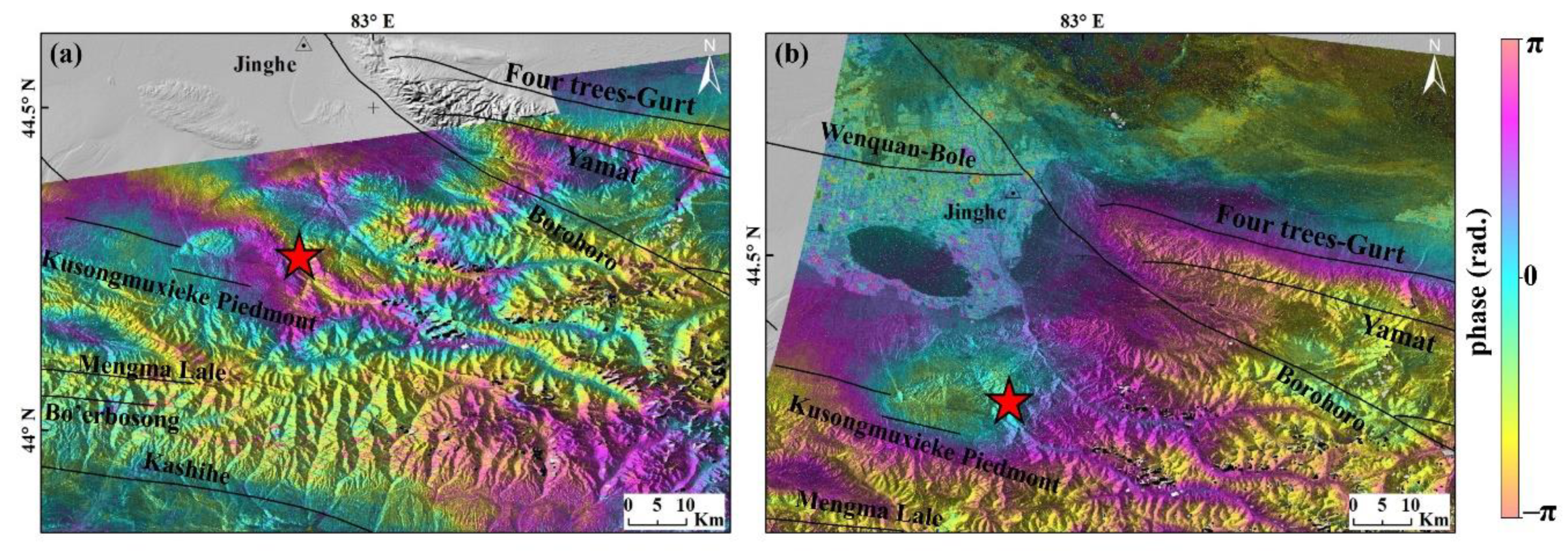
Figure 2.
Examples of interferograms affected by strong atmospheric signals, where red stars denote the epicenter of the Mw 6.3 Jinghe earthquake. (a) Wrapped interferogram from ascending track T12 (4 June 2017–15 August 2017); (b) wrapped interferogram from descending track T165 (8 August 2017–1 September 2017). The scale per one color-cycle is

Figure 3.
Baseline information for four tracks with different viewing geometries; the y-axis denotes the (P-baseline); and x-axis denotes the acquisition dates formatted as yyyy/mm/dd; the gray line denotes the earthquake date. (a) T12 ascending orbit; (b) T63 descending orbit; (c) T85 ascending orbit; (d) T165 descending orbit.

Figure 4.
Reconstructed maps of coseismic displacement in a line-of-sight (LoS) direction. Color scale is from −6.7 to 6.7 cm, and the positive values indicate the movements towards the satellite sensor. (a) Sentinel-1 T12; (b) Sentinel-1 T63; (c) Sentinel-1 T85; (d) Sentinle-1 T165; (e) Advanced Land Observing Satellite 2 (ALOS2) ascending interferogram.

Figure 5.
(a) Locations of candidate fault models overlaid with the local terrain and relocated earthquake sequence derived by Liu et al. [12] (circles); the colors of circles denote quake depths (light to dark corresponding to shallow to deep) and the radius denotes the magnitude. (b) Optimization of the dip angle for the different candidate fault locations.

Figure 6.
Estimated slip distribution of (a) the south dipping model and (b) the north dipping model. Red stars denote the epicenter of the main shock derived from sequence relocation [12]. The x-axis is the distance along the EW direction (units: km) and the y-axis is the vertical depth (units: km).

Figure 7.
Estimated slip distribution for (a) the south dipping model with a strike of 100° and (b) the south dipping model with a strike of 110°. Red stars denote the main shock epicenter derived from sequence relocation [12]. The x-axis is the distance along the strike direction (units: km) and the y-axis is the vertical depth (units: km).

Figure 8.
Quad-tree down-sampled observations (Obs., first line) for each track-orbit, forward modeling results (Mod., second line), and residual (Res., last line) inversion of the south dipping model. From left to right, the results are based on data from T12, T85, T63, T165, and the Advanced Land Observing Satellite2 (ALOS2). All subplots share the color scale shown in the lower right of the figure.

Figure 9.
Model of the genetic mechanism of the 2017 Mw 6.3 Jinghe earthquake. The bold red line denotes the seismogenic fault suggested by this study; the dashed red line denotes the speculative upper part of this fault; the side view of the focal mechanism solution denotes the type of event. KPF—Kusongmuxieke Pediment Fault.

Figure 10.
Coulomb stress change caused by the 2017 Mw 6.3 Jinghe earthquake based on the optimal Interferometric Synthetic Aperture Radar (InSAR) south-dipping distributed slip model. (a–c) Distribution of Coulomb stress change at a depth of 7.5, 15, and 20 km, respectively; (b) cross-section of Coulomb stress change along profile A–B. The red star denotes the epicenter of the 2017 Mw 6.3 Jinghe earthquake derived by InSAR, and the black circle denotes the epicenter of the 2018 Mw 5.2 event [23].


Table 1.
Focal mechanism solutions of the 2017 Mw 6.3 Jinghe earthquake.
| Source a | Lat. (°) | Lon. (°) | Depth (km) | Nodal Plane 1 (°) | Nodal Plane 2 (°) | Mw | ||||
|---|---|---|---|---|---|---|---|---|---|---|
| Strike | Dip | Rake | Strike | Dip | Rake | |||||
| USGS | 82,827 | 44,301 | 20 | 269 | 30 | 87 | 92 | 60 | 92 | 6.3 |
| GCMT | 82,740 | 44,400 | 27.6 | 244 | 52 | 66 | 101 | 44 | 118 | 6.3 |
| CENC | 82,890 | 44,270 | 11.0 | 269 | 47 | 99 | 76 | 44 | 80 | 6.3 |
a USGS—United States Geological Survey; GCMT—Global Centroid Moment Tensor; CENC—China Earthquake Networks Center.
Table 2.
Parameters of the estimated displacement maps from Sentinel 1 and PALSAR2 1.
| Satellite | Track-Orbit 2 | Single Pair Min. SD (cm) | Single Pair Max. SD (cm) | Averaged Disp. SD. (cm) | Heading (Deg.) | Average Inc. (Deg.) | Max. LoS Disp. (cm) |
|---|---|---|---|---|---|---|---|
| S1 | T12A | 1.95 | 3.87 | 1.14 | −10.76 | 33.53 | 6.46 |
| S1 | T85A | 1.86 | 3.35 | 1.27 | −9.32 | 43.3 | 4.88 |
| S1 | T63D | 1.71 | 2.88 | 0.74 | −169.44 | 35 | 5.56 |
| S1 | T165D | 1.48 | 2.32 | 0.81 | −170.83 | 44.26 | 4.51 |
| ALOS2 3 | 880A | 2.44 | 2.97 | 2.44 | −10.89 | 38.7 | 6.42 |
1 SD—standard deviation; LoS—line-of-sight; PALSAR2—Phased Array type L-band Synthetic Aperture Radar 2; ALOS2—Advanced Land Observing Satellite 2. 2 A—ascending orbit; D—descending orbit. 3 Only one ALOS2 pair was used here (that with the lowest SD).
Table 3.
Determined source parameters for the north dipping and south dipping models 1.
| Model | Lon./° | Lat./° | Z/km | Strike | Dip | Rake | Mw |
|---|---|---|---|---|---|---|---|
| InSAR-ND | 82.74 | 44.29 | 16.73 | 270 | 42 | 84.02 | 6.37 |
| InSAR-SD | 82.72 | 44.26 | 14.05 | 90 | 42 | 89.56 | 6.19 |
1 Lon., Lat., and Z denote the locations for the maximum slip; The rake angle is the value at the maximum slip patch of the fault; ND—dipping to the north, striking 270°; SD—dipping to the south, striking 90°; InSAR—Interferometric Synthetic Aperture Radar.
© 2019 by the authors. Licensee MDPI, Basel, Switzerland. This article is an open access article distributed under the terms and conditions of the Creative Commons Attribution (CC BY) license (http://creativecommons.org/licenses/by/4.0/).
Share and Cite
MDPI and ACS Style
Gong, W.; Zhang, Y.; Li, T.; Wen, S.; Zhao, D.; Hou, L.; Shan, X. Multi-Sensor Geodetic Observations and Modeling of the 2017 Mw 6.3 Jinghe Earthquake. Remote Sens. 2019, 11, 2157. https://doi.org/10.3390/rs11182157
AMA Style
Gong W, Zhang Y, Li T, Wen S, Zhao D, Hou L, Shan X. Multi-Sensor Geodetic Observations and Modeling of the 2017 Mw 6.3 Jinghe Earthquake. Remote Sensing. 2019; 11(18):2157. https://doi.org/10.3390/rs11182157
Chicago/Turabian StyleGong, Wenyu, Yingfeng Zhang, Tao Li, Shaoyan Wen, Dezheng Zhao, Liyan Hou, and Xinjian Shan. 2019. "Multi-Sensor Geodetic Observations and Modeling of the 2017 Mw 6.3 Jinghe Earthquake" Remote Sensing 11, no. 18: 2157. https://doi.org/10.3390/rs11182157
Note that from the first issue of 2016, this journal uses article numbers instead of page numbers. See further details here.