Hyperspectral Endmember Extraction Using Spatially Weighted Simplex Strategy

Abstract

Spatial information is increasingly becoming a vital factor in the field of hyperspectral endmember extraction, since it takes into consideration the spatial correlation of pixels, which generally involves jointing spectral information for preprocessing and/or endmember extraction in hyperspectral imagery (HSI). Generally, simplex-based endmember extraction algorithms (EEAs) identify endmembers without considering spatial attributes, and the spatial preprocessing strategy is an independently executed module that can provide spatial information for the endmember search process. Despite this interest, to the best of our knowledge, no one has studied the integration framework of the spatial information-embedded simplex for hyperspectral endmember extraction. In this paper, we propose a spatially weighted simplex strategy, called SWSS, for hyperspectral endmember extraction that investigates a novel integration framework of the spatial information-embedded simplex for identifying endmember. Specifically, the SWSS generates the spatial weight scalar of each pixel by determining its corresponding spatial neighborhood correlations for weighting itself within the simplex framework to regularize the selection of the endmembers. The SWSS could be implemented in the traditional simplex-based EEAs, such as vertex component analysis (VCA), to introduce spatial information into the data simplex framework without the computational complexity excessively increasing or endmember extraction accuracy loss. Based on spectral angle distance (SAD) and root-mean-square-error (RMSE) evaluation criteria, experimental results on both synthetic and $Cuprite$ real hyperspectral datasets indicate that the simplex-based EEA re-implemented by the SWSS has a significant improvement on endmember extraction performance over the techniques on their own and without re-implementing.

1. Introduction

Hyperspectral remote sensing is related to the extraction of information from objects or scenes lying on the Earth’s surface, based on their radiance acquired by airborne or spaceborne sensors [1,2]. Hyperspectral sensing, or spectral imaging, has been motivated in extracting increasingly detailed information about the material properties of pixels in a scene for agricultural, biomedical, industrial, civilian, and military applications, since the sensor can acquire a spectral vector with hundreds or thousands of elements from every pixel to provide valuable information towards such materials in this scene [3,4,5,6,7]. However, since the spatial resolution of a sensor is coarser than the scale of spatial heterogeneity of the ground surface, the pixels that mix with many different disparate substances are inevitably contained in HSI [8,9]. Moreover, when a mixing model assumes to be of linear type such that the incident light interacts with one material, the process that decomposes the measured spectrum of a mixed pixel into a collection of constituent spectra, or $\mathit{endmembers}$, and a set of corresponding fractions, or $\mathit{abundances}$, can be defined as spectral unmixing (SU) [3,9]. As such, for the above-mentioned applications in the field of hyperspectral remote sensing, endmembers normally correspond to familiar macroscopic material in the scene, such as water, soil, metal, vegetation, etc. [5], and the SU can be seen as an ability to discriminate the distribution of endmembers in a realistic situation.

Generally, endmember extraction has attracted more attention in SU because the endmember is a pre-condition for estimating abundance. Current algorithms for endmember extraction can be divided into four primary categories, namely pure pixel assumption-based algorithms [10,11,12,13,14,15,16], non-pure pixel assumption-based algorithms [17,18,19,20,21], statistical algorithms [22,23], and sparse regression-based algorithms [24,25]. However, pure pixel assumption-based algorithms have probably been the most often used in SU owing to their light computational burden and clear conceptual meaning [9]. They generally assume that there is at least one pure pixel per endmember on the vertex to define a data simplex. Therefore, they generally focus on one of the following geometric properties: (1) the endmember corresponds to an extreme projection on a subspace; or (2) the endmember corresponds to the spectral signatures that can define a maximum simplex volume. In this regard, the endmember extraction can be seen as an identification of pure pixels extracted from the HSI. Representative pure pixel assumption-based algorithms could be mainly divided into two parts, given as follows.

(1)

Extreme projection-based approaches: The extreme projection-based approaches explore the property that the vertices of the simplex, i.e., endmembers, could capture the extreme values when they are projected onto a determined direction vector or a subspace. Preliminary work in this field focused primarily on the pixel purity index (PPI) [10]. PPI projects all the spectral vectors onto randomly generated $skewers$ (i.e., random direction spectral vectors), and the desired endmembers are determined by counting the number of times spectral vectors are found to have the extreme values. Unlike the PPI, the orthogonal subspace projection (OSP) approach [11] and vertex component analysis (VCA) [14] iteratively select the endmember by projecting entire spectral vectors onto a direction orthogonal to the subspace spanned by the already determined endmembers. It is worth mentioning that projection-based methods also play a crucial role in other fields, such as image corner detection [26] or image registration [27].

(2)

Maximum simplex volume-based approaches: the maximum simplex volume-based approaches are based on the fact that the volume formed by the vertices of the simplex is larger than any other volume defined by the interior pixels within the simplex. N-FINDR [12] is classic maximum simplex volume-based algorithm that identifies the endmembers by searching a set of spectral vectors within the HSI that can specify a maximum volume. Simplex growing algorithm (SGA) [15] comprise another well-known method that begins with two vertices and begins to grow a simplex by increasing its vertices one at a time until reaching the terminated number of vertices. Inspired by N-FINDR, alternating volume maximization (AVMAX) [19] is presented for endmember extraction, where the volume of the simplex is defined by the endmembers with respect to only one endmember at one time.

For most of aforementioned EEAs, their quantitative and comparative analysis can be found in ref. [28]. Here, we will refer to the extreme projection- and maximum simplex volume-based approaches as simplex-based approaches since both criteria use the convexity of the hyperspectral data structure.

However, most of the above-mentioned algorithms are spectrally oriented, resulting in the intrinsic spatial attribute of the endmember being ignored and thus the data simplex becoming sensitive to anomalies. Specifically, according to the Tobler’s first law of geography that "Everything is related to everything else, but near things are more related than distant things" [29], the endmembers extracted within the HSI should be spectrally similar to their neighborhoods. However, anomalies are special patterns in data without a well-defined notion of normal behavior [30], and their signatures are spectrally distinct from their surroundings or background representation [31]. Such anomalies are potentially generated during detector failure, data transfer, and improper data correction [32]. When anomalies occur in the HSI, they are more likely to be selected as endmembers since such anomalies may force a vertex of the simplex to reside at a point beyond the nominal position of the endmember in order to enclose every point [5].

Hyperspectral imagery is conceptually a two-dimensional pictorial representation of the ground surface, with both spatial and spectral attributes [8]. As such, despite the truth of the spectral features of anomalies being distinct from their surroundings, the anomalies tend to be characterized spatially when their spatial neighbors’ correlation is taken into account. On the basis of taking spatial and spectral features into consideration simultaneously, several spatial information-assisted algorithms are presented from the point of view of spatial–spectral-based EEAs and spatial preprocessing strategy, respectively. The spatial–spectral-based EEAs combine spatial and spectral information for identifying endmembers directly without considering the properties of the data simplex. The original spatial–spectral-based EEA appears in automated morphological endmember extraction (AMEE) [33], which governs two classic mathematical morphology operators, erosion, and dilation. An erosion operation selects the most highly mixed pixel, while a dilation operation determines the purest pixel. Under this circumstance, a morphological eccentricity index (MEI) is defined to generate endmembers by an iterative process. The spatial preprocessing strategies generally involve the process of using both spatial and spectral features with the specific intent of offering a few high-quality pixels for fast endmember extraction. The first systematic study on spatial preprocessing strategy was carried out in 2009 by Plaza [34], i.e., spatial preprocessing algorithm (SPP). In this study, a spatial scalar factor is used to weigh the importance of the spectral information associated with each pixel in terms of its spatial context. Later, in ref. [35], Martín and Plaza present another outstanding work, i.e., spatial-spectral preprocessing algorithm (SSPP), which fuses spatial and spectral information by selecting a subset of spatially homogeneous and spectrally pure pixels from each cluster for endmember extraction. It is worth mentioning that the spatial preprocessing strategies are an efficient measure with which to provide spatial information for the spectral-based algorithms such as simplex-based algorithms, because those spatial preprocessing strategies heavily depend upon an assumption that the endmembers are more likely to be found in spatially homogeneous areas, where the pixels derived from the same homogeneous area are spatially close and spectrally similar [34]. Unfortunately, such spatial preprocessing strategies are an independent module prior to the spectral-based EEAs.

To summarize, several conclusions follow.

(1)

For the simplex-based algorithms, the spatial attributes of the endmembers are not in the spotlight and thus the simplex-based algorithms fall into the trap of the anomaly.

(2)

In the field of spatial preprocessing strategies, they are an independently executed module separate from the spectral-based EEA.

(3)

The spatial attributes of the endmembers may lie in the fact that the endmembers are more likely to be found in homogeneous areas, implying that the endmember extracted within the HSI should be spatially close and spectrally similar to its neighborhoods.

To the best of our knowledge, no one has studied the integration framework of the spatial information-embedded simplex for hyperspectral endmember extraction. This paper proposes a novel strategy, termed SWSS, that discusses how to incorporate spatial information into a simplex, such as extreme projection and the maximum simplex volume criterion-based simplex. First, the SWSS generates a spatial weight scalar for each pixel by calculating their spatial neighborhood correlations. Then, the determined spatial weight scalar is used to weight the pixel itself within the simplex framework for regularizing the selection of the endmembers. Unlike the traditional simplex-based algorithms or the spatial preprocessing strategies, the SWSS provide a spatial information-embedded simplex framework for identifying endmembers from both spatial and spectral viewpoints. Therefore, the SWSS shows its novelty in three ways.

(1)

Spatial information is captured to regularize the selection of endmembers within the simplex in the spectral domain.

(2)

The effectiveness of the simplex can be highly retained without computation complexity excessively increasing or endmember extraction accuracy loss.

(3)

The robustness of the simplex-based algorithms to anomalies could be boosted.

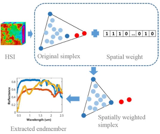
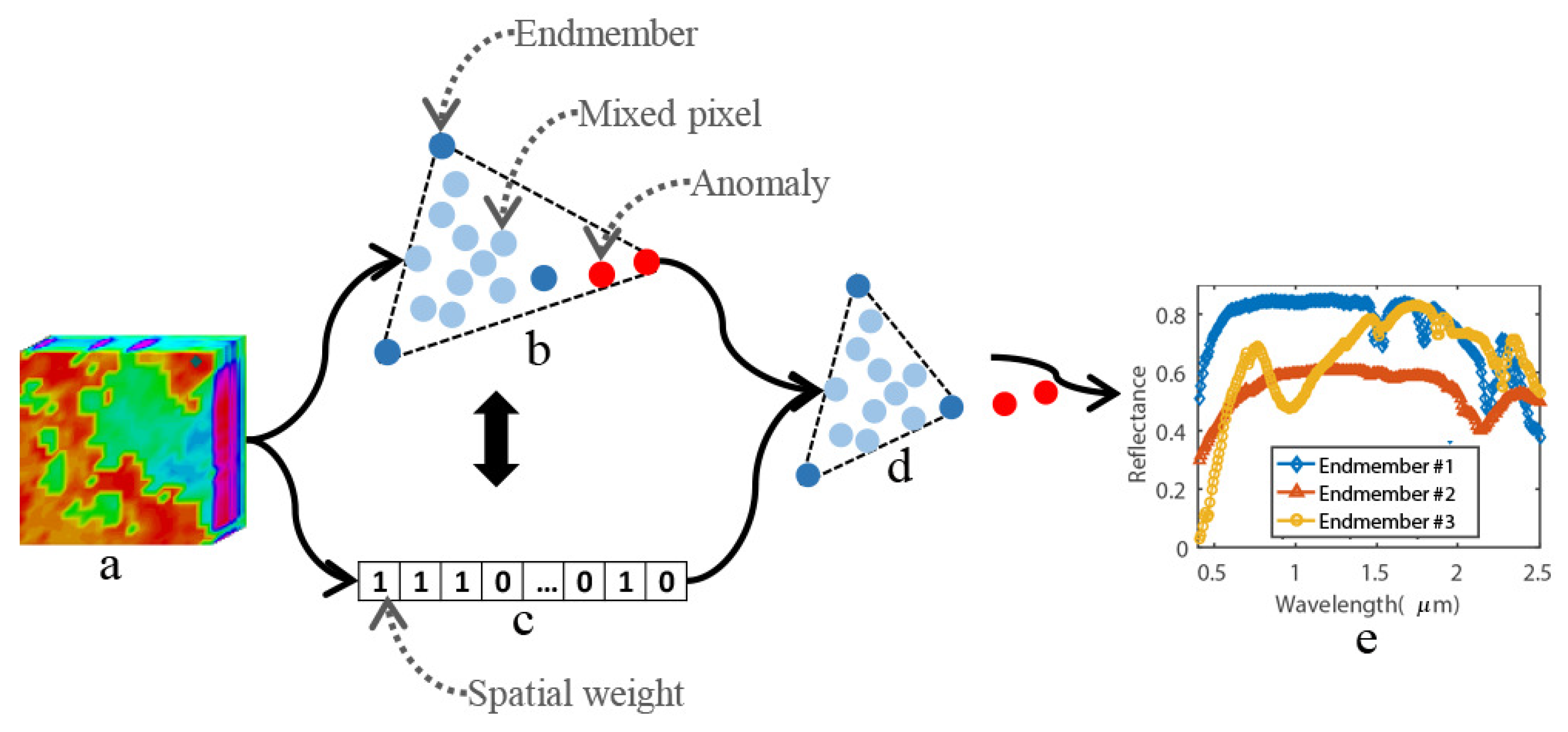
To display the SWSS in detail, a flowchart is given in Figure 1. As we can see, the traditional data simplex is sensitive to anomalies (marked as red spheres), but the data simplex can be regularized after each pixel within the data simplex is weighted by its spatial weight scalar.

Section 2 gives a brief overview of the research background with respect to LMM and geometric properties. Then, the SWSS is outlined in Section 3. Several experiments conducted on different hyperspectral dataset are presented in Section 4. Our conclusions are drawn in the final section.

2. Background

This section gives a brief review of the background that the SWSS relies on. First, the linear mixing model (LMM) is introduced in Section 2.1, which is the basis model of the SU associated with endmembers and abundances. Then, the geometric properties that the traditional simplex-based algorithms basically lie in are presented in Section 2.2.

2.1. LMM

Despite many studies taking into consideration a nonlinear mixing model (NLMM) that is based on the assumption of physical interactions between the light scattered by multiple materials, the past decades have also witnessed a huge growth in the LMM, which assumes that the mixing scale is macroscopic and the incident light interacts with just one material [9]. Owing to the chief reason that the LMM has an acceptable approximation for the light scattering type, the LMM has been widely used to address SU problems, i.e., the process of estimating the endmembers and the abundances.

Let $\mathbf{Y}=[{\mathit{y}}_{\mathbf{1}},{\mathit{y}}_{\mathbf{2}},\dots ,{\mathit{y}}_{\mathit{n}}]\in {\mathbb{R}}^{B\times n}$ be a measured hyperspectral image, the LMM can be given by

$$\mathbf{Y}=\mathbf{M}\mathbf{A}+\mathit{\omega },$$

(1)

where $\mathbf{M}=[{\mathit{m}}_1,{\mathit{m}}_2,\dots ,{\mathit{m}}_p]\in {\mathbb{R}}^{\mathit{B}\times \mathit{p}}$ stands for the endmember matrix, $\mathbf{A}={[{\mathit{\alpha }}_1,{\mathit{\alpha }}_2,\dots ,{\mathit{\alpha }}_n]}^T\in {\mathbb{R}}^{\mathit{p}\times \mathit{n}}$ stands for the abundance fraction matrix, $\mathit{\omega }\in {\mathbb{R}}^{\mathit{B}\times \mathit{n}}$ accounts for the additive noise matrix. Moreover, $\mathit{B}$ and $\mathit{n}$ denote the spectral bands and total number of image pixels, respectively. $\mathit{p}$ denotes the number of endmembers, which can be estimated by classic techniques, e.g., virtual dimensionality (VD) [36]. Two different constraints, the abundance non-negativity constraint (ANC), i.e., ${\mathit{\alpha }}_{\mathit{i}}⪰0$, and the abundance sum-to-one constraint (ASC), i.e., ${\mathbf{1}}^{\mathit{T}}{\mathit{\alpha }}_i=1$ ($\mathbf{1}$ is a vector of ones), for $i=1,\dots ,n$, are imposed on the abundance fraction matrix.

2.2. Geometric Properties

With the previously mentioned [3,9] in mind, a great deal of EEAs have focused on geometric properties of the hyperspectral data, which involves an extreme projection criterion, maximum simplex volume criterion, and minimum simplex volume criterion [17]. Unlike the minimum simplex volume criterion, the first two criteria determine endmembers from within image spectra and their corresponding models are formulated below.

2.2.1. Extreme Projection Criterion

Based on the LMM, Equation (1) can be re-implemented as follows:

$$\mathbf{Y}={\mathit{e}}_{\mathit{p}}{\alpha }_p+{\mathbf{U}}_{\mathit{p}-\mathbf{1}}{\mathit{\zeta }}_{\mathit{p}-\mathit{1}}+\mathit{\omega },$$

(2)

where ${\mathit{e}}_{\mathit{p}}={\mathit{m}}_{\mathit{p}}$ is a desired endmember, ${\mathbf{U}}_{\mathit{p}-\mathbf{1}}=[{\mathit{m}}_{\mathbf{1}},{\mathit{m}}_{\mathbf{2}},\dots ,{\mathit{m}}_{\mathit{p}-\mathbf{1}}]$ is the endmember matrix with remaining $\mathit{p}-1$ undesired endmember signatures, and the potential corresponding abundance of ${\mathbf{U}}_{\mathit{p}-\mathbf{1}}$ is ${\mathit{\zeta }}_{\mathit{p}}-\mathbf{1}$. According to ref. [11], the OSP classifier projector is given as follows:

$${\mathbf{P}}_{\mathit{OSP}}={\mathbf{P}}_{{\mathbf{U}}_{\mathit{p}-\mathbf{1}}}^{\perp }{\mathit{e}}_{\mathit{p}},$$

(3)

where ${\mathit{P}}_{{\mathbf{U}}_{\mathit{p}-\mathbf{1}}}^{\perp }=\mathbf{I}-{\mathbf{U}}_{\mathit{p}-\mathbf{1}}{\left({\mathbf{U}}_{\mathit{p}-\mathbf{1}}^{\mathbf{T}}{\mathbf{U}}_{\mathit{p}-\mathbf{1}}\right)}^{-1}{\mathbf{U}}_{\mathit{p}-\mathbf{1}}^{\mathbf{T}}$ denotes the orthogonal subspace projector, and $\mathbf{I}$ denotes an identity matrix.

2.2.2. Maximum Simplex Volume Criterion

Based on the pure pixel assumption, the endmembers correspond to the spectral signatures that can define a maximum simplex volume with the vertices specified by other pixels. Let $\mathit{V}\left({\mathit{y}}_{{\mathit{k}}_{\mathbf{1}}},{\mathit{y}}_{{\mathit{k}}_{\mathbf{2}}},\cdots ,{\mathit{y}}_{{\mathit{k}}_{\mathit{p}}}\right)$ be the simplex volume with respect to ${\mathit{y}}_{{\mathit{k}}_{\mathbf{1}}},{\mathit{y}}_{{\mathit{k}}_{\mathbf{2}}},\cdots ,{\mathit{y}}_{{\mathit{k}}_{\mathit{p}}}$, and the simplex volume can be defined by

$$\mathit{V}\left({\mathit{y}}_{{\mathit{k}}_{\mathbf{1}}},{\mathit{y}}_{{\mathit{k}}_{\mathbf{2}}},\cdots ,{\mathit{y}}_{{\mathit{k}}_{\mathit{p}}}\right)=\mathit{abs}\left(\left|\begin{array}{cccc}1& 1& \cdots & 1\\ {\mathit{y}}_{{\mathit{k}}_{\mathbf{1}}}& {\mathit{y}}_{{\mathit{k}}_{\mathbf{2}}}& \cdots & {\mathit{y}}_{{\mathit{k}}_{\mathit{p}}}\end{array}\right|\right)/\left(p-1\right)!,$$

(4)

where ${\mathit{y}}_{{\mathit{k}}_{\mathbf{1}}},{\mathit{y}}_{{\mathit{k}}_{\mathbf{2}}},\cdots ,{\mathit{y}}_{{\mathit{k}}_{\mathit{p}}}$ are the pixels that are selected from $\mathbf{Y}$. More detailed analysis can be seen in the literature [12].

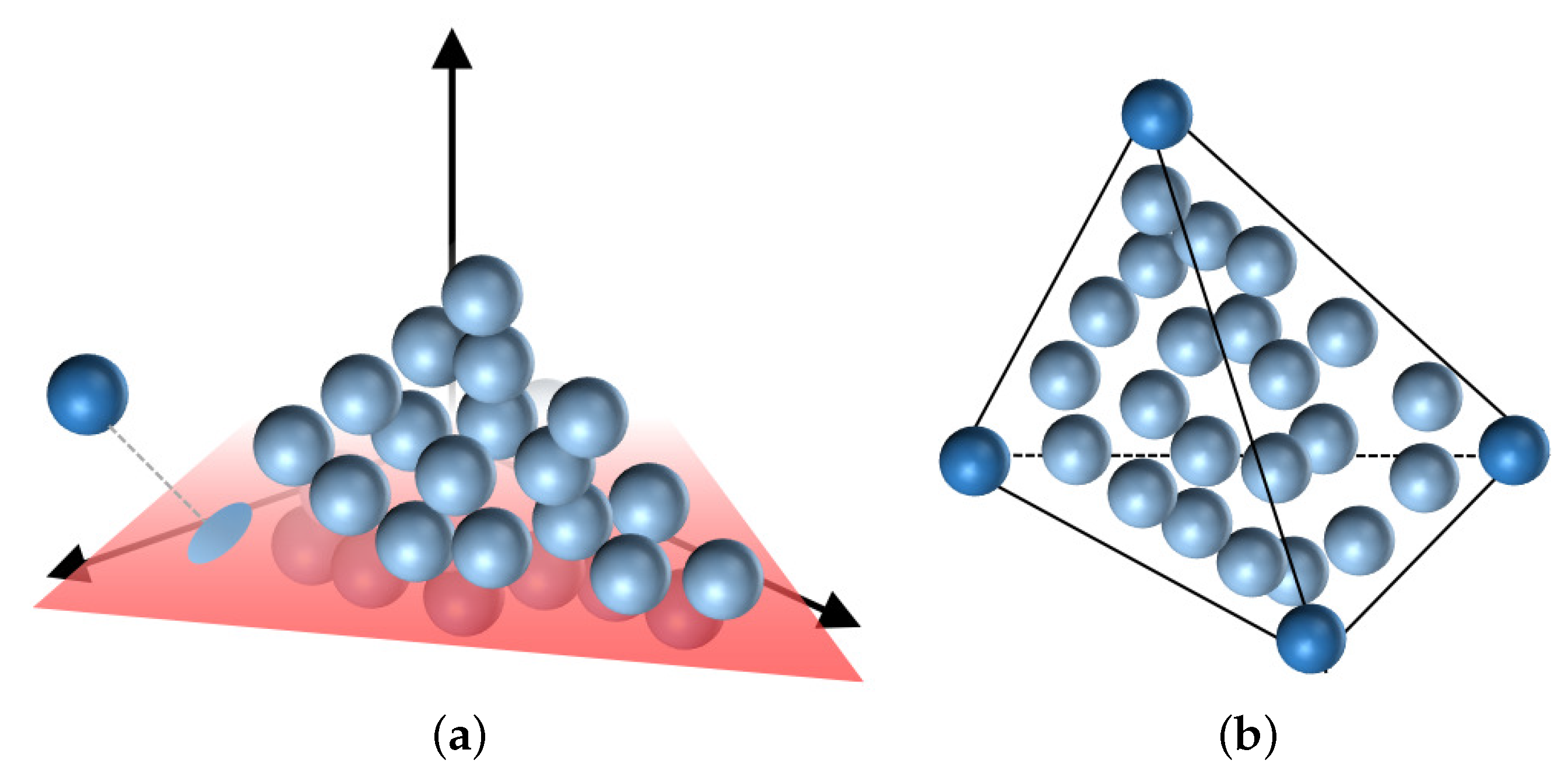
A 3-dimensional illustration of the simplex is given in Figure 2.

3. Materials and Methods

Keeping the preceding expression in mind, this section concentrates on the SWSS. First, the SWSS generates a spatial weight scalar for each pixel by calculating their spatial neighborhood correlations. Then, the determined spatial weight scalar is used to weight the pixel itself within the simplex framework for regularizing the selection of the endmembers. Figure 1 illustrates the SWSS in detail. As we can see from this image, the traditional simplex does not take spatial attributes of the vertices (i.e., endmembers) into consideration, resulting in one of the vertexes being seized by the anomaly. However, due to the reason that the spatial weight scalar is introduced, it can be used to weight the pixels within the traditional simplex for endmember extraction.

3.1. Spatial Information Exploitation

This section describes the process of the spatial information exploitation, which refers to two parts. First, we use the well-known singular value decomposition (SVD) technique to denoise the HSI. Then, we use local window method to capture the neighborhood correlations of target pixels and yield their corresponding spatial weight scalar under the denoised hyperspectral data.

3.1.1. SVD for Denoising

Normally, when the HSI suffers from the poor noise interference, the spatial information of the HSI may be difficultly characterized. Therefore, the SVD method is first used to alleviate the noise interference. According to Equation (1), the SVD of the data matrix of $\mathbf{Y}$ is a decomposition of the following form:

$$\mathbf{Y}=\mathsf{\Theta }\mathsf{\Sigma }{\mathsf{\Lambda }}^T=\sum _{i=1}^n{\sigma }_i{\mathit{\theta }}_i{\mathit{\lambda }}_i^T,$$

(5)

where $\mathsf{\Theta }=\left[{\mathit{\theta }}_1,{\mathit{\theta }}_2,\dots ,{\mathit{\theta }}_n\right]\in {\mathbb{R}}^{B\times n}$ and $\mathsf{\Lambda }=\left[{\mathit{\lambda }}_1,{\mathit{\lambda }}_2,\dots ,{\mathit{\lambda }}_n\right]\in {\mathbb{R}}^{n\times n}$ are the matrices with orthonormal columns, i.e., ${\mathsf{\Theta }}^T\mathsf{\Theta }={\mathsf{\Lambda }}^T\mathsf{\Lambda }=\mathbf{I}$, and where $\mathsf{\Sigma }=\mathrm{diag}\left({\sigma }_1,{\sigma }_2,\dots ,{\sigma }_n\right)\in {\mathbb{R}}^{n\times n}$ is the diagonal matrix and the diagonal elements are singular values of $\mathsf{\Sigma }$ such that

$${\sigma }_1\ge {\sigma }_2\ge \cdots \ge {\sigma }_n\ge 0.$$

(6)

Theoretically, the SVD can divide the data space into true signal and noise subspaces pertaining to separate sets of singular values [37]. Let q be the rank of noise-free hyperspectral data, i.e., $\mathbf{M}\mathbf{A}$, and the denoised data matrix can be given by

$$\widehat{\mathbf{Y}}=\sum _{i=1}^q{\widehat{\sigma }}_i{\mathit{\theta }}_i{\mathit{\lambda }}_i^T,$$

(7)

where $\widehat{\mathbf{Y}}=[{\widehat{\mathit{y}}}_{\mathbf{1}},{\widehat{\mathit{y}}}_{\mathbf{2}},\dots ,{\widehat{\mathit{y}}}_{\mathit{n}}]\in {\mathbb{R}}^{B\times n}$ denotes the denoised hyperspectra data, and ${\widehat{\sigma }}_i$ denotes the singular value matrix such that ${\sigma }_1\ge {\sigma }_2\ge \cdots \ge {\sigma }_q\ge 0$ and ${\sigma }_{q+1}={\sigma }_{q+2}=\cdots ={\sigma }_n=0$.

3.1.2. Local Window for Characterizing Spatial Neighborhood Correlation

For the denoised hyperspectral imagery $\widehat{\mathbf{Y}}$, the local window is then used to calculate spatial neighborhood correlation using the SAD. For the ${\widehat{\mathit{y}}}_{\mathit{i}}$, its spatial neighborhood correlations of ${\widehat{\mathit{y}}}_{\mathit{i}}$ can be defined as follows:

$${\mathit{s}}_{\mathit{i}}=\mathit{l}/\sum _{{\widehat{\mathit{y}}}_{\mathit{i}}^{\mathit{neighbor}}\in \mathcal{N}}arccos\left({\widehat{\mathit{y}}}_{\mathit{i}}^{\mathit{T}}{\widehat{\mathit{y}}}_{\mathit{i}}^{\mathit{neighbor}}\right./∥{\widehat{\mathit{y}}}_{\mathit{i}}∥∥{\widehat{\mathit{y}}}_{\mathit{i}}^{\mathit{neighbor}}∥),$$

(8)

where $s_i$ denotes the spatial neighborhood correlations of ${\widehat{\mathit{y}}}_{\mathit{i}}$, $\mathit{l}$ denotes the number of neighbor pixels in a neighbor system, $\mathcal{N}$ denotes the neighbor system centered in ${\widehat{\mathit{y}}}_{\mathit{i}}$, and ${\widehat{\mathit{y}}}_{\mathit{i}}^{\mathit{neighbor}}$ is the neighboring pixel of ${\widehat{\mathit{y}}}_{\mathit{i}}$ encapsulated in $\mathcal{N}$, $\mathit{i}=1,2,\dots ,\mathit{l}$.

Based on the determined spatial neighborhood correlations of each pixel, we define $\mathit{S}={[{\mathit{s}}_1,{\mathit{s}}_2,\dots ,{\mathit{s}}_{\mathit{n}}]}_{\mathit{n}\times 1}$ as a spatial correlation matrix for characterizing the inherent spatial information of each pixel in the hyperspectral data. It is worth noting that when the spatial correlation between a given pixel and its neighbor pixels is high, the values of ${\mathit{s}}_{\mathit{i}}$ will be relatively large. Furthermore, when there are anomalies, their spatial neighbor correlations are weak, which indicates that their corresponding spatial correlations are low as well. In this regard, for further characterizing the neighborhood correlations of each pixel, a threshold $\delta$ is used to segment the neighborhood correlations of pixels. This can be defined as follows:

$${\mathit{w}}_{\mathit{i}}=\left\{\begin{array}{cc}1\hfill & {\mathit{s}}_{\mathit{i}}\ge \delta \hfill \\ 0\hfill & {\mathit{s}}_{\mathit{i}}<\delta .\hfill \end{array}\right.$$

(9)

The threshold $\delta$ could segment the spatial correlation matrix $\mathit{S}$ into a spatial weight matrix $\mathit{W}={[{\mathit{w}}_1,{\mathit{w}}_2,\dots ,{\mathit{w}}_{\mathit{n}}]}_{\mathit{n}\times 1}$ with 0 or 1 values, where 1 denotes the right spatial neighborhood correlations that the pixel is and 0 denotes the quite contrary meaning. In other words, only the spatial weight of pixels with high spatial correlation, such as homogeneous pixels, will be set to 1, yet the anomalies or heterogeneous pixels will be set to 0.

3.2. Spatially Weighted Simplex

With the previous brief overview of the geometric properties and the defined spatial weight in mind, this section investigates the different joint types between the spatial information of pixels and the data simplex.

3.2.1. Spatially Weighted Extreme Projection Criterion

For the extreme projection-based simplex, the endmembers are sequentially extracted by finding the extreme projections of the pixels lie on the orthogonal subspace spanned by the already determined endmembers. Therefore, for the projections of all pixels, their spatial weight partners with their corresponding projections for determining endmembers. The first endmember can be determined by the following formulation:

$${\mathit{e}}_{\mathbf{1}}=\underset{{\mathit{y}}_{\mathit{i}}}{argmin}\left({\mathit{w}}_{\mathit{i}}{\mathit{y}}_{\mathit{i}}^{\mathit{T}}{\mathit{y}}_{\mathit{i}}\right),$$

(10)

where ${\mathit{e}}_{\mathbf{1}}$ is the first endmember, and ${\mathit{w}}_{\mathit{i}}$ denotes the spatial weight of the pixel ${\mathit{y}}_{\mathit{i}}$. Likewise, the other endmembers can be iteratively determined as follows:

$${\mathit{e}}_{\mathit{p}}=\underset{{\mathit{y}}_{\mathit{i}}}{argmin}\left({\mathit{w}}_{\mathit{i}}{\mathit{P}}_{{\mathbf{U}}_{\mathit{p}-\mathbf{1}}}^{\perp }{\mathit{y}}_{\mathit{i}}\right),$$

(11)

where ${\mathit{e}}_{\mathit{p}}$ denotes the $p$-th extracted endmember, ${\mathbf{U}}_{\mathit{p}-\mathbf{1}}=[{\mathit{e}}_{\mathbf{1}},{\mathit{e}}_{\mathbf{2}},\dots ,{\mathit{e}}_{\mathit{p}-\mathbf{1}}]$, ${\mathit{P}}_{{\mathbf{U}}_{\mathit{p}-\mathbf{1}}}^{\perp }=\mathbf{I}-{\mathbf{U}}_{\mathit{p}-\mathit{1}}{\left({\mathbf{U}}_{\mathit{p}-\mathbf{1}}^{\mathit{T}}{\mathbf{U}}_{\mathit{p}-\mathbf{1}}\right)}^{-1}{\mathbf{U}}_{\mathit{p}-\mathbf{1}}^{\mathit{T}}$, and $\mathbf{I}$ denotes the identity matrix. According to Equations (10) and (11), the role played by the ${\mathit{w}}_{\mathit{i}}$ within the extreme projection-based simplex is that only the projections of the pixels with low spatial neighborhood correlations are ignored, but retaining the projections of the pixels with high spatial neighborhood correlations without itself being changed.

3.2.2. Spatially Weighted Maximum Simplex Volume Criterion

For the maximum volume-based simplex, the endmembers are extracted simultaneously. Hence, when pixels are used to define a simplex volume, their corresponding spatial weights should be taken into consideration simultaneously. In this regard, the spatially weighted maximum volume-based simplex is implemented as follows:

$$\mathit{V}\left({\mathit{y}}_{{\mathit{k}}_{\mathbf{1}}},{\mathit{y}}_{{\mathit{k}}_{\mathbf{2}}},\cdots ,{\mathit{y}}_{{\mathit{k}}_{\mathit{i}}},\cdots ,{\mathit{y}}_{{\mathit{k}}_{\mathit{p}}}\right)=\prod _{\mathit{i}=1}^{\mathit{p}}{w}_{k_i}\mathit{abs}\left(\left|\begin{array}{cccccc}1& 1& \cdots & 1& \cdots & 1\\ {\mathit{y}}_{{\mathit{k}}_{\mathbf{1}}}& {\mathit{y}}_{{\mathit{k}}_{\mathbf{2}}}& \cdots & {\mathit{y}}_{{\mathit{k}}_{\mathit{i}}}& \cdots & y_{k_p}\end{array}\right|\right)/\left(p-1\right)!,$$

(12)

where ${\mathit{y}}_{{\mathit{k}}_{\mathbf{1}}},{\mathit{y}}_{{\mathit{k}}_{\mathbf{2}}},\cdots ,{\mathit{y}}_{{\mathit{k}}_{\mathit{i}}},\cdots ,{\mathit{y}}_{{\mathit{k}}_{\mathit{p}}}$ are pixels derived from $\mathbf{Y}$, and their corresponding spatial weight are ${\mathit{w}}_{{\mathit{k}}_1},{\mathit{w}}_{{\mathit{k}}_2},\dots ,{\mathit{w}}_{{\mathit{k}}_{\mathit{i}}},\dots ,{\mathit{w}}_{{\mathit{k}}_{\mathit{p}}}$, respectively. Obviously, when the pixels are used to calculate a simplex volume, their corresponding spatial weight are cumulatively multiplied for weighting the volume. Once there exists at least one pixel with a spatial weight of 0 value, the simplex volume will be set to 0 as well.

In conclusion, this section presents the process of how the SWSS works. Specifically, based on the determined spatial weight from the noise removal and the spatial neighborhood correlation viewpoint, the pixels are regularized to specify the endmembers within the simplex. Therefore, in the SWSS, the pixels with low spatial neighborhood correlations such as anomalies, are masked, but the pixels with high spatial neighborhood correlations are more likely to be selected as endmembers.

4. Results

This section describes the experimental results conducted on synthetic and real hyperspectral datasets. To evaluate the effectiveness of the SWSS on the different simplex-based algorithms, the SWSS was implemented in four state-of-the-art algorithms $\mathit{original} \mathit{version}$, i.e., OSP, N-FINDR, VCA, and AVMAX, which all involve extreme projection and the maximum volume criterion.

Their $\mathit{improved} \mathit{versions}$ were named SWSS-OSP, SWSS-N-FINDR, SWSS-VCA, and SWSS-AVMAX, respectively, and their performances in different experimental scenarios were compared to those of their original versions. Furthermore, as the well-known spatial preprocessing strategy, the SPP was used to combine with the four original simplex-based algorithms to validate the performance of the improved versions.

For the SWSS, we carefully tuned the parameters regarding neighbor system size and segmentation thresholds. Neighbor system size was used to enclose a set of neighboring pixels to calculate the spatial correlation between the central pixel and its corresponding neighboring pixels. In the subsequent experiments, the neighbor system $\mathcal{N}$ was set to a square neighbor block with different sliding windows varying in size from 3 to 9. In our experiment, $ws$ denotes the window size, and $ws$ could fixed to 3, 5, 7, and 9. Furthermore, the classic OTSU [38] algorithm was adapted to automatically determine the segmentation threshold $\delta$ for segmenting spatial information into spatial weight with values of 0 or 1. Owing to the dataset having multiple scenarios, such as different noise situations, anomaly situations, and the selection of window size $ws$, the threshold results are too many and thus are given in

Table 1. The segmentation $\delta$ specified by the OTSU algorithm; it was used to segment the spatial information of each pixel of the synthetic image (without anomalies) under different SNRs and window sizes $ws$.

Window Size	ws = 3	ws = 5	ws = 7	ws = 9
10 dB	0.3647	0.4314	0.4549	0.4706
20 dB	0.3686	0.4431	0.4353	0.4078
30 dB	0.2863	0.3490	0.3804	0.3961
40 dB	0.2510	0.3255	0.3647	0.3686
50 dB	0.2196	0.3118	0.3314	0.3059
60 dB	0.2588	0.3176	0.3255	0.3333

,

Table 2. The segmentation threshold $\delta$ specified by the OTSU algorithm; it was used to segment the spatial information of each pixel of the synthetic image (with anomalies) under different SNRs and window sizes $ws$.

Window Size	ws = 3	ws = 5	ws = 7	ws = 9
10 dB	0.4667	0.5294	0.5373	0.5294
20 dB	0.4000	0.4549	0.4784	0.4588
30 dB	0.2980	0.3804	0.3961	0.4157
40 dB	0.2627	0.3333	0.3647	0.3725
50 dB	0.2431	0.2784	0.3275	0.3353
60 dB	0.2118	0.3137	0.3294	0.3431

and

Table 3. The segmentation $\delta$ specified by the OTSU algorithm; it was used to segment the spatial information of each pixel on the $Cuprite$ dataset under different window sizes $ws$.

Window Size	ws = 3	ws = 5	ws = 7	ws = 9
$\delta$	0.1882	0.1882	0.1804	0.1686

. In addition, the first $\mathit{p}$ singular values were retained to denoise the HSI; $\mathit{p}$ denotes the number of estimated endmembers. For the SPP, its window size is fixed to 3 and 5 in the synthetic dataset and real dataset, respectively, since it can provide good results in the image considered [34].

4.1. Evaluation Metrics

Two benchmarking evaluation metrics, i.e., SAD [28] and root-mean-square error (RMSE) [5], were used to evaluate the experimental performance of all considered algorithms. The SAD is widely used to compare the spectral similarity between extracted endmembers and their corresponding library spectra:

$$\mathit{SAD}\left({\mathit{y}}_{\mathit{i}},{\mathit{y}}_{\mathit{j}}\right)=arccos\left({\mathit{y}}_{\mathit{i}}^{\mathit{T}}{\mathit{y}}_{\mathit{j}}/∥{\mathit{y}}_{\mathit{i}}∥∥{\mathit{y}}_{\mathit{j}}∥\right),$$

(13)

where ${\mathit{y}}_{\mathit{i}}$ and ${\mathit{y}}_{\mathit{j}}$ denote two different spectra. The greater the spectral similarity between ${\mathit{y}}_{\mathit{i}}$ and ${\mathit{y}}_{\mathit{j}}$, the smaller the SAD. RMSE is another metric used to calculate the reconstruction error between the original and the reconstructed hyperspectral image. It can be given by

$$\mathit{RMSE}\left(\mathit{Y},\tilde{\mathit{Y}}\right)={\left(\frac{1}{B\times n}\sum _{i=1}^n{\left({\mathit{y}}_{\mathit{i}}-{\tilde{\mathit{y}}}_{\mathit{i}}\right)}^2\right)}^{\frac{1}{2}},$$

(14)

where $\mathit{B}$ and $\mathit{n}$ denote the spectral bands and total number of image pixels, respectively, and the ${\mathit{y}}_{\mathit{i}}$ and ${\tilde{\mathit{y}}}_{\mathit{i}}$ are derived from the original HSI $\mathbf{Y}$ and the reconstructed HSI $\tilde{\mathbf{Y}}$ (specified by the extracted endmembers and estimated abundances), respectively. The lower the RMSE, the better the reconstruction performance. Similarly, the lower the RMSE, the better the reconstruction performance.

4.2. Experiments on Synthetic Datasets

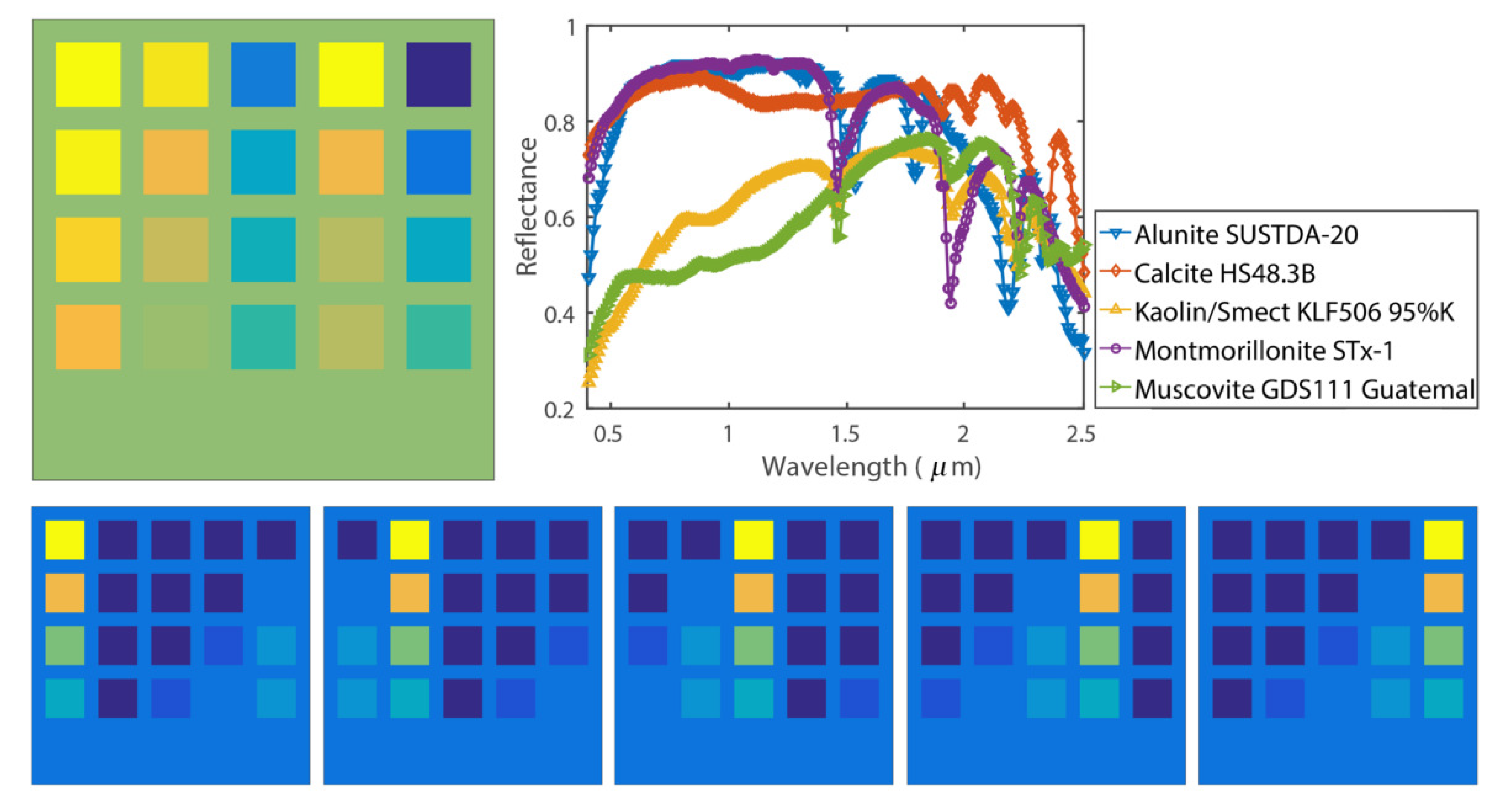
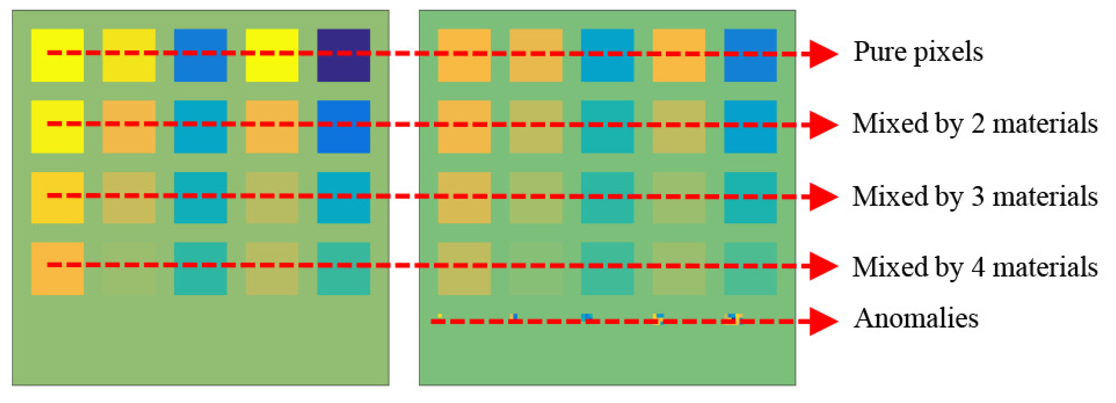
In this experiment, five endmembers were randomly selected from the United States Geological Survey (USGS) spectral library (Http://Speclab.Cr.Usgs.Gov/Spectral.Lib06) with 224 bands, namely Alunite SUSTDA-20, Calcite HS48.3B, Kaolin/Smect KLF506 95%K, Montmorillonite STx-1, and Muscovite GDS111 Guatemal. Furthermore, the LMM along with the ANC and ASC were used to generate a 100 × 100-pixel synthetic image. Zero mean white Gaussian noise was added to the synthetic images with signal-to-noise ratios (SNRs) varying from 10 dB to 60 dB. Here, based on the above-mentioned synthetic dataset design, two different synthetic datasets were provided to evaluate the performance of the algorithms. The first synthetic dataset did not take an anomaly into account, and this synthetic dataset with its corresponding five signatures and abundances can be seen from Figure 3. It is worth mentioning that the synthetic image was comprised of multiple blocks filled by mixed pixels with different spectral purities: i.e., 1 (pure pixels ), 0.8 (mixed with 2 materials), 0.6 (mixed with 3 materials), and 0.4 (mixed with 4 materials) (Figure 4). Additionally, the background of the image was made up of mixed pixels averaged on all endmembers (the purity of each material was 0.2).

To validate the performance of the algorithms in a more realistic scenario, the second synthetic dataset was designed based on the first synthetic dataset. In the second synthetic dataset, several anomalies were added to the image (Figure 4). According to Equation (2), we formulate an anomaly spectrum $\mathit{a}$ as follows [9]:

$$\mathit{a}={\mathit{m}}_{\mathit{p}}\gamma +{\mathbf{U}}_{\mathit{p}-\mathbf{1}}{\mathit{\zeta }}_{\mathit{p}-\mathbf{1}}+\mathit{\omega },$$

(15)

where $\gamma$ denotes the abundance fraction of a desired target spectrum ${\mathit{m}}_{\mathit{p}}$, and is randomly determined in the interval [1, 1.2]. $\gamma +{\mathbf{1}}^{\mathit{T}}{\mathit{\zeta }}_{\mathit{p}-\mathbf{1}}=1$, where $\mathbf{1}$ is a $\mathit{p}\times 1$ vector of ones. In order to generate different simulated anomaly areas, five panels of different sizes were added to the image. The sizes were 1 × 1, 2 × 2, 2 × 3, 3 × 3, and 3 × 5.

4.2.1. Experiment 1: Comparison between Original and Improved Versions Under Different Noise Scenarios

The purpose of Experiment 1 is to provide a comparison between the original and improved algorithms under different noise scenarios.

Table 4. SAD results of the original and improved versions, with the experiment conducted on a synthetic image (without anomalies) under different SNRs.

Algorithms	OSP	SWSS-OSP	N-FINDR	SWSS-N-FINDR	VCA	SWSS-VCA	AVMAX	SWSS-AVMAX
10 dB	0.4327	0.4212	0.4170	0.4030	0.1166	0.0826	0.4199	0.3991
20 dB	0.1475	0.1587	0.1417	0.1411	0.0316	0.0223	0.1399	0.1396
30 dB	0.0457	0.0450	0.0453	0.0449	0.0092	0.0078	0.0448	0.0447
40 db	0.0143	0.0143	0.0156	0.0150	0.0029	0.0026	0.0143	0.0141
50 dB	0.0045	0.0044	0.0047	0.0045	0.009	0.0008	0.0045	0.0045
60 dB	0.0014	0.0014	0.0018	0.0018	0.0003	0.0003	0.0014	0.0017
Average	0.1077	0.1081	0.1044	0.1011	0.0269	0.0201	0.1041	0.1006

and

Table 5. SAD results of the original and improved versions for experiments conducted on a synthetic image (with anomalies) under different SNRs.

Algorithms	OSP	SWSS-OSP	N-FINDR	SWSS-N-FINDR	VCA	SWSS-VCA	AVMAX	SWSS-AVMAX
10 dB	0.4214	0.4212	0.4270	0.4030	0.1245	0.0826	0.4263	0.4044
20 dB	0.1798	0.1543	0.1568	0.1386	0.0581	0.0213	0.1555	0.1385
30 dB	0.0776	0.0456	0.0791	0.0444	0.0603	0.0074	0.0725	0.0442
40 db	0.0625	0.0141	0.0537	0.0152	0.0558	0.0025	0.0557	0.0141
50 dB	0.0553	0.0044	0.0465	0.0046	0.0555	0.0009	0.0546	0.0044
60 dB	0.0549	0.0014	0.0527	0.0014	0.0548	0.0003	0.0509	0.0014
Average	0.1419	0.1068	0.1360	0.1011	0.0665	0.0192	0.1359	0.1012

present the SAD results on two synthetic dataset situations under different noise scenarios varying from 10 to 60 dB, respectively. As Table 4 shows, the SAD results of the improved and original versions were very close. Further analysis showed that the improved algorithm did not decrease the endmember extraction accuracy. As shown in Table 5, the most remarkable result is that the original versions fell into the trap of anomalies, whereas the improved versions maintained endmember extraction accuracy.

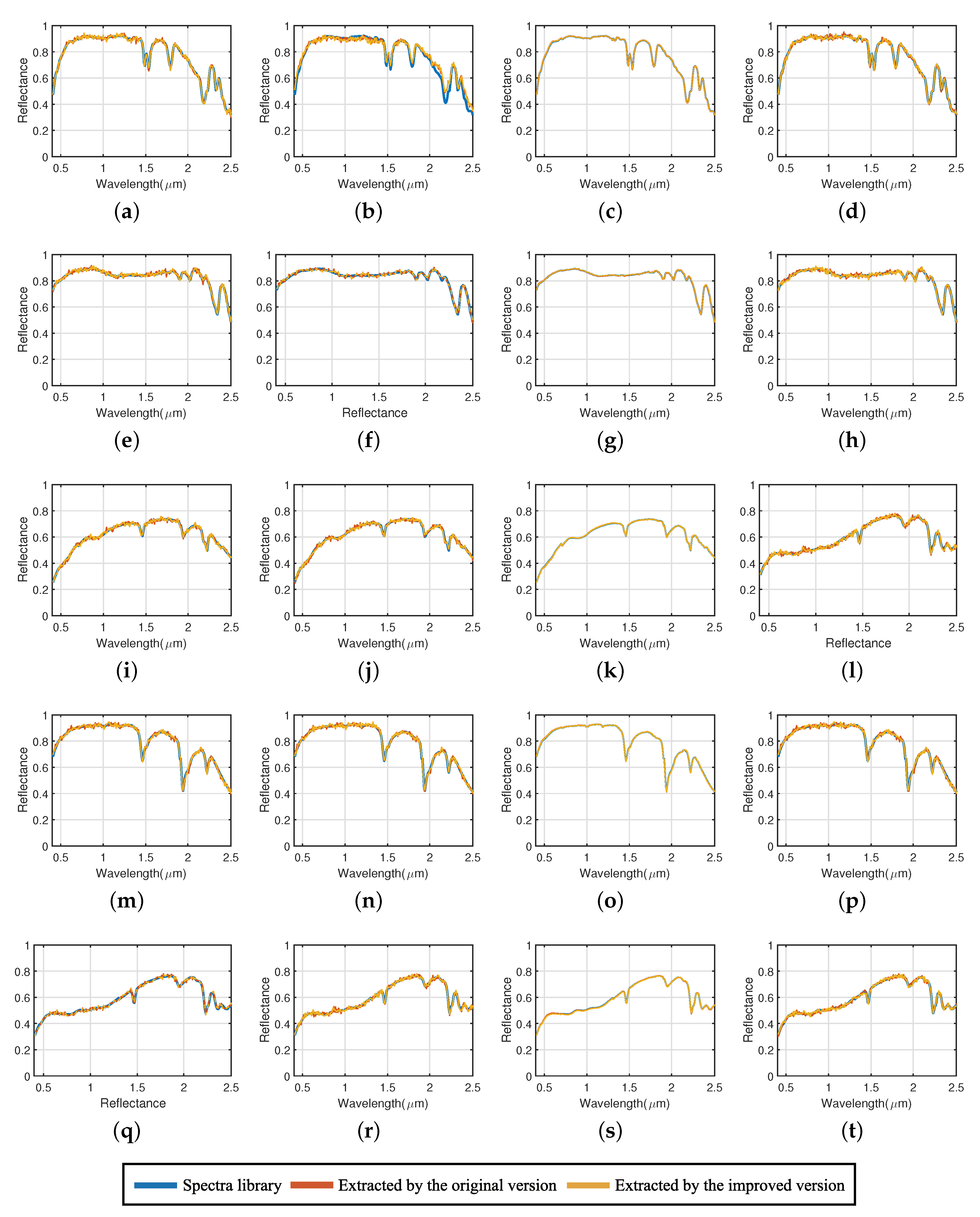
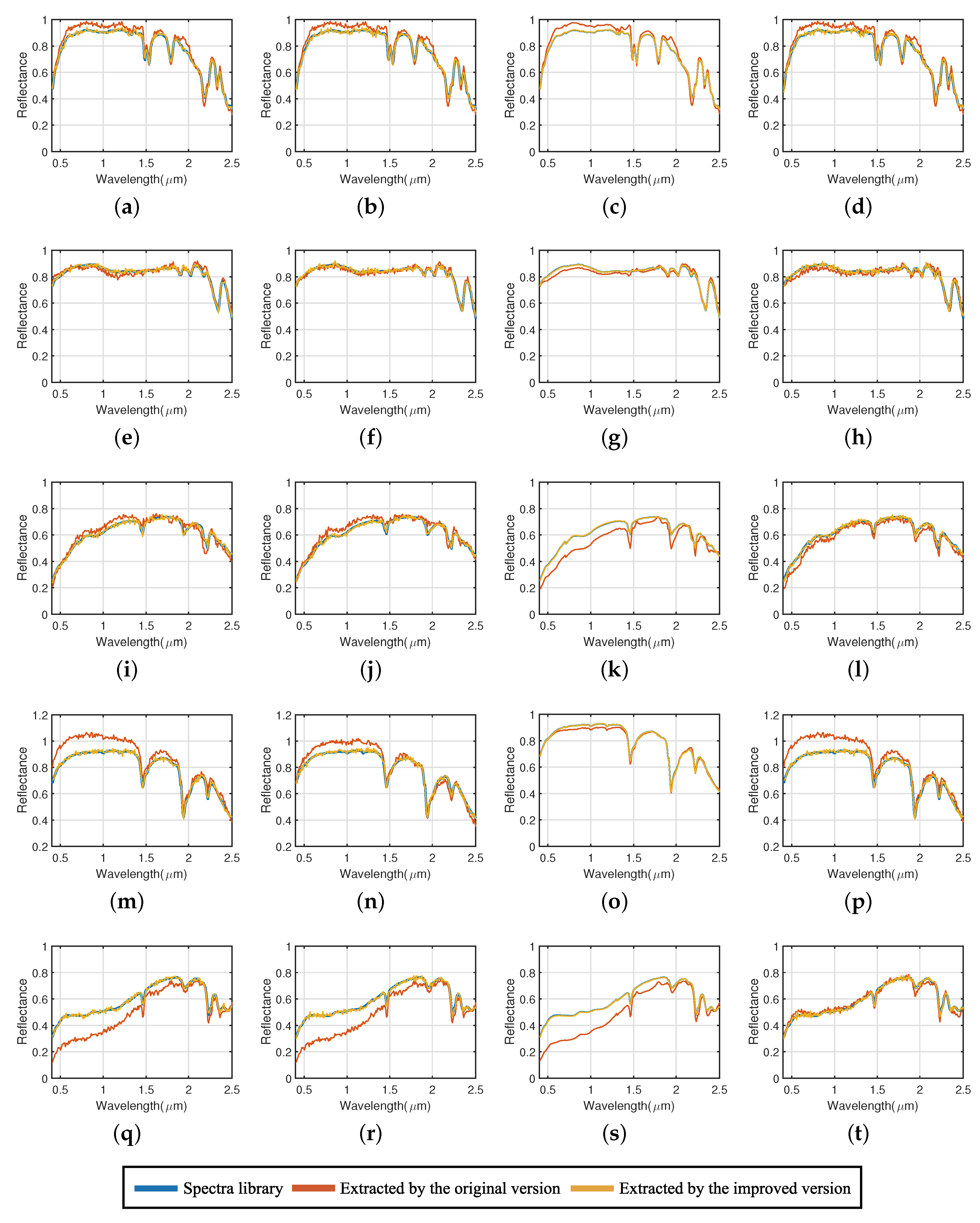
Additionally, for the 40-dB case with $ws$ fixed to 7, both Figure 5 and Figure 6 visually compare the spectra library and the extracted endmembers derived from the original and improved algorithms. Figure 5 is based on the synthetic image without anomalies, and Figure 6 is based on the image with embedded anomalies. As can be seen from Figure 5, the endmembers extracted by the original and improved version closely matched the spectra library. However, for the synthetic image that took into consideration anomalies, Figure 6 shows that the endmembers identified by the improved version remained highly similar to spectra library whereas the endmembers determined by the original version were different from the spectra library. This result further strengthened our confidence in the SWSS since it can enhance the robustness of the simplex-based algorithm and avoid the interference of anomalies.

4.2.2. Experiment 2: Comparison of and Improved Versions Under Different Window Size Scenarios

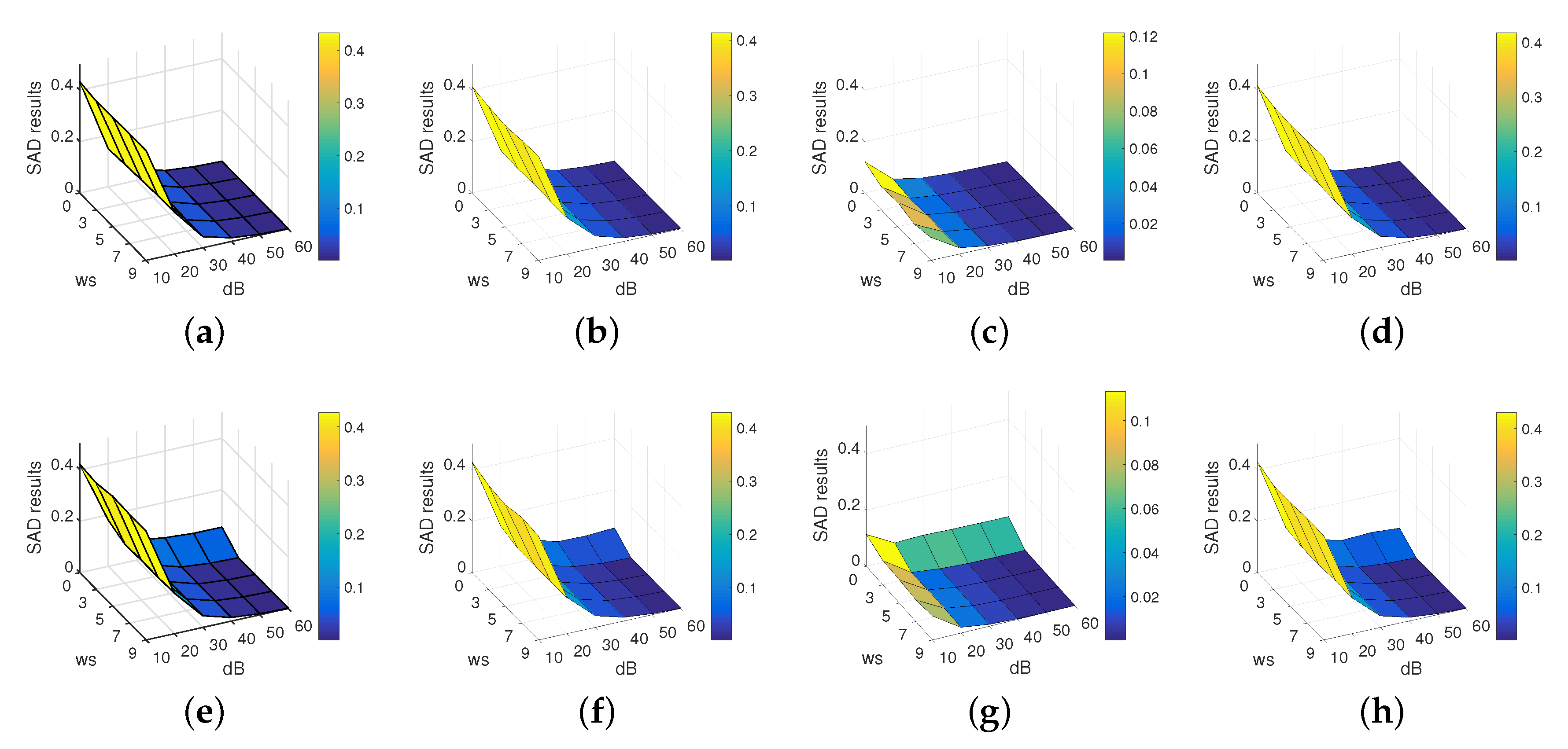
To assess the impact of window size,

Table 6. SAD results and execution time (tabulated in parentheses) obtained from the improved versions under different window sizes $ws$ and in two synthetic dataset scenarios.

Window Size	ws = 3	ws = 5	ws = 7	ws = 9
SWSS-OSP	0.1069 (6.7327)	0.1081 (10.1887)	0.1085 (14.1675)	0.1087 (20.8113)
SWSS-N-FINDR	0.1010 (4.3943)	0.1003 (7.8081)	0.1010 (12.3514)	0.1021 (18.3483)
SWSS-VCA	0.0204 (3.9102)	0.0215 (7.3713)	0.0178 (11.9351)	0.0207 (17.9347)
SWSS-AVMAX	0.1005 (3.6717)	0.1006 (7.0336)	0.1003 (11.6494)	0.1011 (17.5922)
Average	0.0822 (4.6772)	0.0826 (8.1004)	0.0819 (12.6751)	0.0831 (18.6714)
SWSS-OSP${}^{\mathsf{\S }}$	0.1052 (7.0531)	0.1078 (10.3613)	0.1070 (14.7728)	0.1074 (20.6785)
SWSS-N-FINDR${}^{\mathsf{\S }}$	0.1013 (4.7310)	0.996 (7.8970)	0.1023 (12.3459)	0.1016 (18.3418)
SWSS-VCA${}^{\mathsf{\S }}$	0.0195 (4.2739)	0.0195 (7.4921)	0.0184 (11.9772)	0.0193 (17.9635)
SWSS-AVMAX${}^{\mathsf{\S }}$	0.1006 (3.9692)	0.1005 (7.1675)	0.1020 (11.6026)	0.1016 (17.6000)
Average${}^{\mathsf{\S }}$	0.0817 (5.0068)	0.0818 (8.2292)	0.0824 (12.6746)	0.0825 (18.6460)

${}^{\mathsf{\S }}$ denotes results obtained from synthetic dataset with anomalies added.

also tabulates the SAD results and execution times under different window sizes for the four improved algorithms conducted on two different synthetic datasets. In this table, when $ws$ = 7, the four improved algorithms have the lowest average SAD results on the synthetic dataset without anomalies added; meanwhile, their average exaction times were highest when $ws$ = 9. For the synthetic dataset with anomalies added, when $ws$ was fixed to 3, the four improved versions could generate relatively better average SAD results compared to other window sizes. Looking at Figure 7, it is apparent that the execution time is highly associated with the window size. The larger the window size, the greater the execution time of the improved versions will be. This may be because the large window size involves many dot-product operations.

4.2.3. Experiment 3: Joint Consideration of Different Window Size and Noise Scenarios between Original and Improved Versions

To provide a tendency of the SAD results under different combination of the window size and noise scenarios, Experiment 3 is performed by the original and improved versions on the both synthetic datasets. As shown in Figure 8, when no anomalies exist in the synthetic dataset, the original ($ws$ equals to 0) and improved versions ($ws$ varies from 3 to 9) show a visually same tendency of the SAD results. However, when the anomalies are added to the synthetic dataset, the improved versions show a better tendency of the SAD results, while the original versions do not.

4.2.4. Experiment 4: Comparison between SPP Coupled Simplex-Based Algorithms and Improved Versions Under Different Noise and Synthetic Scenarios

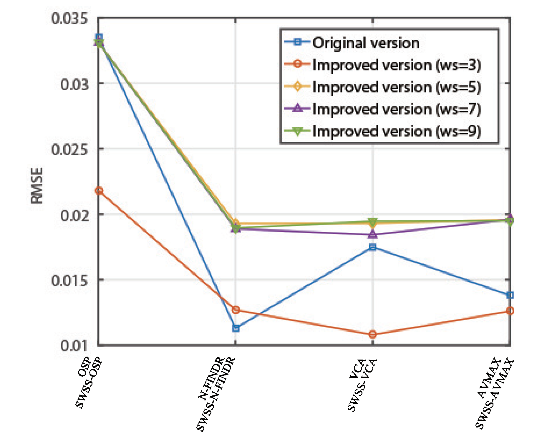
The aim of Experiment 4 is to evaluate the performance of the spatial preprocessing strategy, i.e., SPP coupled simplex-based algorithms, and of the improved versions.

Table 7. SAD results captured from SPP coupled algorithms and improved versions under different noise and synthetic dataset scenarios.

SNRs	10 dB	20 dB	30 dB	40 dB	50 dB	60 dB
SPP+OSP	0.1859	0.1091	0.0503	0.0297	0.0178	0.0104
SWSS-OSP	0.4216	0.1527	0.0467	0.0144	0.0045	0.0014
SPP+N-FINDR	0.1618	0.0922	0.0525	0.0326	0.0184	0.0106
SWSS-N-FINDR	0.4004	0.1389	0.0447	0.0157	0.0045	0.0015
SPP+VCA	0.0858	0.0593	0.0426	0.0285	0.0173	0.0103
SWSS-VCA	0.0899	0.0205	0.0085	0.0025	0.0009	0.0003
SPP+AVMAX	0.1662	0.0891	0.0509	0.0299	0.0180	0.0105
SWSS-AVMAX	0.3999	0.1372	0.0447	0.0142	0.0045	0.0024
SPP+OSP${}^{\mathsf{\S }}$	0.1837	0.1176	0.0531	0.0301	0.0177	0.0103
SWSS-OSP${}^{\mathsf{\S }}$	0.4129	0.1518	0.0463	0.0142	0.0045	0.0014
SPP+N-FINDR${}^{\mathsf{\S }}$	0.1669	0.0891	0.0554	0.0329	0.0189	0.0104
SWSS-N-FINDR${}^{\mathsf{\S }}$	0.4038	0.1378	0.0445	0.0159	0.0045	0.0014
SPP+VCA${}^{\mathsf{\S }}$	0.0884	0.0565	0.0424	0.0283	0.0173	0.0102
SWSS-VCA${}^{\mathsf{\S }}$	0.0860	0.0193	0.0081	0.0026	0.0010	0.0003
SPP+AVMAX${}^{\mathsf{\S }}$	0.1659	0.0919	0.0500	0.0307	0.0177	0.0103
SWSS-AVMAX${}^{\mathsf{\S }}$	0.4023	0.1379	0.0440	0.0138	0.0044	0.0014

${}^{\mathsf{\S }}$ denotes the results obtained from synthetic dataset with anomalies added.

compares the SAD results captured from the SPP coupled simplex-based algorithms and improved versions under different noise and synthetic scenarios. This table is quite revealing in several ways. First, the improved versions could provide better SAD results in both synthetic datasets, regardless of whether the synthetic dataset contains an anomaly. Second, the SPP coupled simplex-based algorithms display the better SAD results in both synthetic datasets under low-SNR situations, such as 10 and 20 dB, because the SPP can smooth the HSI and alleviate the bad noise or interference from an anomaly prior to endmember extraction. However, the data simplex structure may be influenced when the data is spatially smoothed, resulting in the higher SAD results in high-SNR scenarios compared to the improved versions. Figure 7 visually presents the execution-time results, indicating that the execution times of the improved versions suffer from the window size and the SPP has less computational cost when the window size equals 3.

4.3. Experiment on the Real Dataset

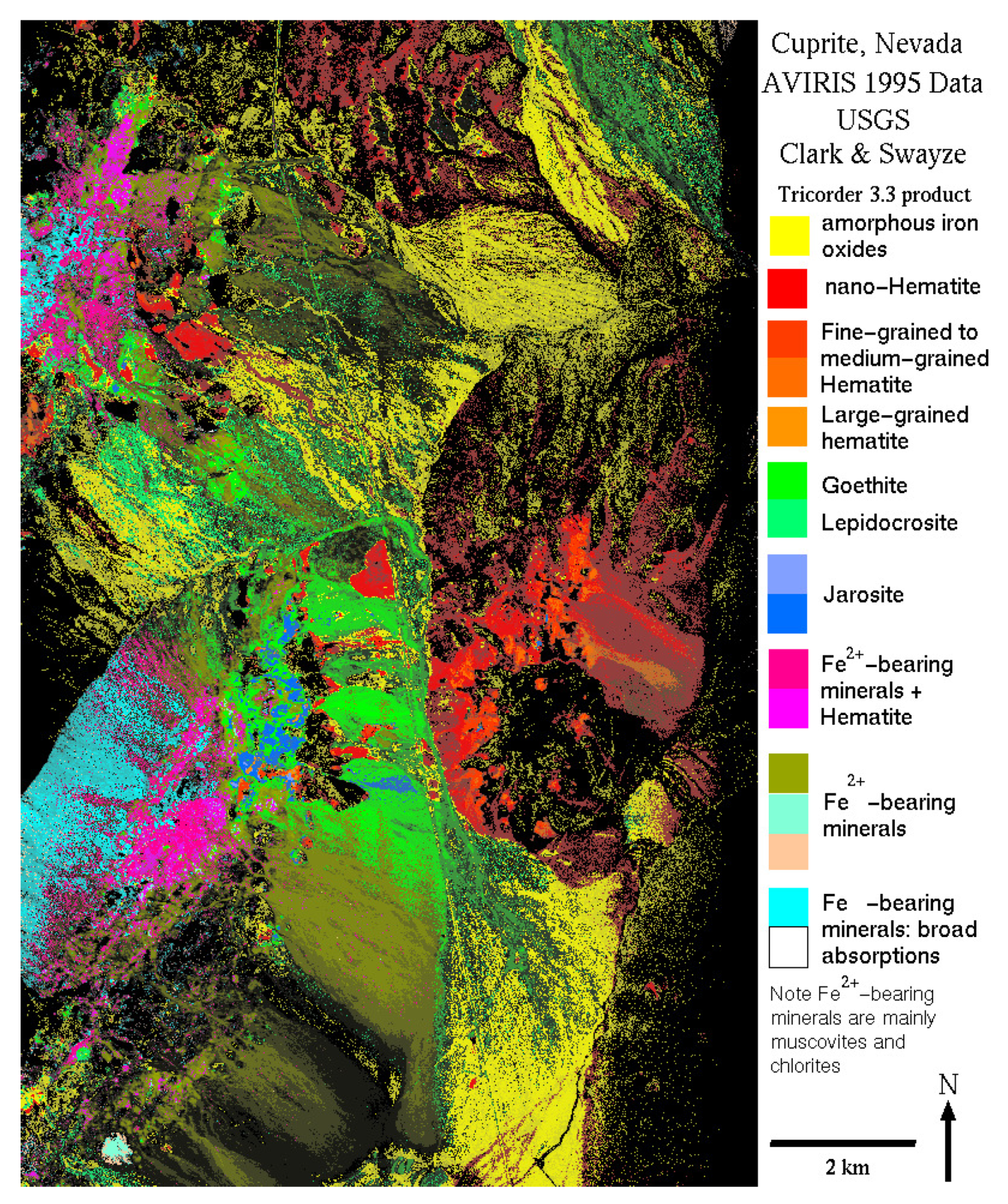
$Cuprite$ is a well-known benchmarking hyperspectral dataset, with data captured by the Airborne Visible Infrared Imaging Spectrometer (AVIRIS). It is used for verifying the performance of hyperspectral unmixing (Figure 9). A 250 × 190 pixel subset with 188 bands was used in this experiment (the noise and water absorption bands were removed from 224 bands, and the excluded bands were 1–2, 104–113, 148–167, and 221–224) http://aviris.jpl.nasa.gov/html/aviris.freedata.html. Based on the analysis in the literature [39], 12 minerals are considered in the experiment, namely $Alunite$, $Andradite$, $Buddingtonite$, $Dumortierite$, $Kaolinite$#1, $Kaolinite$#2, $Muscovite$, $Montmorillonite$, $Nontronite$, $Pyrope$, $Sphene$, and $Chalcedony$. More importantly, we empirically observed that $ws$ fixed to 3 generally provided good results; further analysis is presented later. Subsequent experiments were thus conducted on this window size. The different window sizes and their corresponding threshold $\delta$ values are displayed in Table 3.

In

Table 8. Overall results of the algorithms for experiments conducted on the $Cuprite$ dataset.

Algorithms	OSP	SPP + OSP	SWSS-OSP	N-FINDR	SPP + N-FINDR	SWSS-N-FINDR	VCA	SPP + VCA	SWSS-VCA	AVMAX	SPP + AVMAX	SWSS-AVMAX
Alunite	0.0859	0.1053	0.0955	0.0969	0.1086	0.0955	0.0957	0.1062	0.0944	0.1060	0.1053	0.0955
Andradite	†	0.0843	0.0990	0.0802	0.0813	0.0707	0.0691	0.0742	0.0694	0.0730	0.0713	0.0675
Buddingtonite	0.1159	0.1152	0.0865	0.0775	0.0921	0.0930	0.0734	0.1157	0.1216	0.0862	0.1152	0.1206
Dumortierite	0.0802	0.0681	0.0760	0.0760	0.0680	0.0760	0.0759	0.0674	0.0765	0.0780	0.0675	0.0760
Kaolinite #1	0.0848	0.1047	0.1159	0.0848	†	0.1159	0.0841	0.0903	†	0.0848	0.0908	0.1159
Kaolinite #2	0.0852	0.0653	0.0727	0.0695	0.0671	0.0596	†	0.0701	0.0887	0.0602	0.0699	0.0773
Muscovite	0.0892	0.0962	0.0892	0.0923	0.0962	0.0892	0.0914	0.0954	0.0879	0.0821	0.0912	0.0892
Montmorillonite	0.0618	0.0611	0.0618	0.0612	0.0600	0.0612	0.0647	0.0642	0.0628	0.0618	0.0600	0.0618
Nontronite	0.0736	0.0810	0.0767	0.0736	0.0810	0.0767	0.0774	†	0.0781	0.1068	0.0847	0.0767
Pyrope	†	†	0.0735	†	†	0.1051	†	†	0.0659	†	†	0.0671
Sphene	0.0655	†	†	†	†	†	0.0654	0.0914	†	†	†	†
Chalcedony	0.0870	0.1228	0.1328	0.1003	0.1360	0.1326	0.1144	0.1376	†	0.0933	0.1399	0.0812
Average SAD	0.0829	0.0904	0.0890	0.0812	0.0878	0.0887	0.0812	0.9124	0.0828	0.0832	0.0896	0.0901
RMSE	0.0335	0.0410	0.0218	0.0113	0.0347	0.0127	0.0175	0.0269	0.0108	0.0138	0.0354	0.0126
Execution time	39.2514	61.2759	51.9905	12.8841	61.0445	25.7246	1.1903	53.6188	11.3288	0.5569	52.8609	10.8062

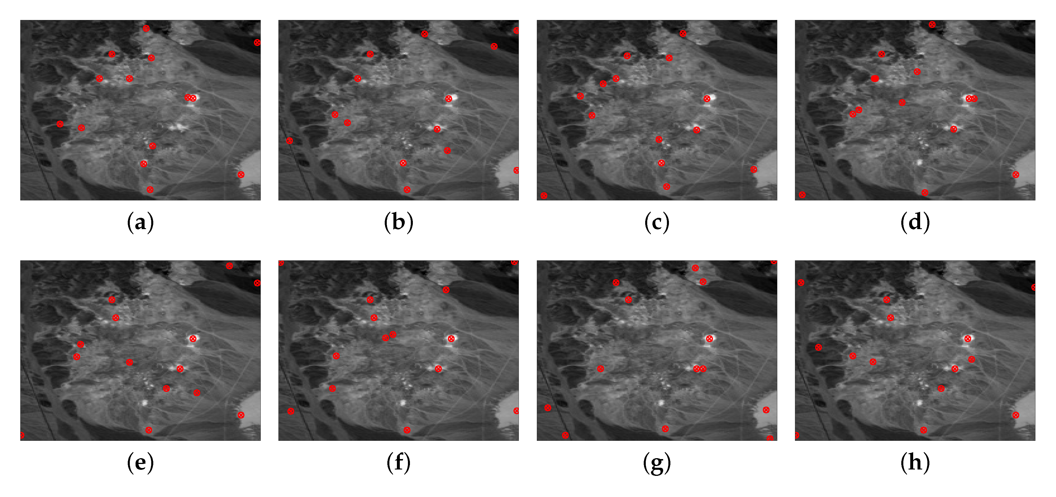
† denotes that the mineral is missed.

, the overall results are displayed in detail, including SAD results, RMSE results, and execution time. Several interesting results are found. First, for several minerals, e.g., Alunite, Muscovite, and Pyrope, most of the improved versions could present better endmember extraction accuracy. Most of the original versions can provide best endmember estimation for Kaolinite #1, Nontronite, and Chalcedony. Dumortierite and Montmorillonite can be perfectly estimated by the most of the SPP coupled simplex-based algorithms. Second, according to the RMSE results, the improved versions could yield lower image reconstruction errors (i.e., RMSE results), especially for SWSS-OSP, SWSS-VCA, and SWSS-AVMAX. Furthermore, in order to analyze the impact of different window size, the best RMSE results generated by the original and improved versions for window sizes of 3, 5, 7, and 9 are displayed in Figure 10. From this figure, when the window size increases, the RMSE values increase as well, indicating that the SWSS may be not valid in such large window-size situations when the method is conducted on the $Cuprite$ dataset. The execution times of these algorithms are tabulated in Table 8, from which it is apparent that the improved versions require approximately 10 s more execution time than the original versions. More importantly, the location of the extracted endmembers derived from the original and improved versions are marked in Figure 11.

5. Discussion

One of the main goals of this experiment was to attempt to assess the usefulness and persistence of the integration framework of the spatial information-embedded simplex under different scenarios. Our result has further strengthened our conviction that the SWSS is a useful spatial information-embedded simplex, which can boost the ability of traditional simplex-based algorithms for endmember extraction by introducing spatial information without an excessive increase in computational cost.

The traditional simplex-based algorithms are advantageous in endmember extraction efficiency, but they suffer from the mistakenly extracted endmembers if a dataset contains an anomaly. However, the preprocessing strategy, e.g., SPP, can alleviate the noise and anomaly interference by spatially smoothing the HSI prior to endmember extraction, yet it still requires more computational time, especially in a real dataset. The SWSS in our paper attempts to capture the superiority of the traditional simplex and the materiality of spatial information, forming a spatial information-embedded simplex. The results offer invaluable evidence that the SWSS could balance the trade-off between endmember extraction efficiency and spatial attributes of endmembers.

One downside regarding our methodology is that the SWSS may be difficult to implement in the minimum volume-based simplex model for covering non-pure pixel assumption-based datasets. Because the non-pure pixel assumption-based simplex models involve the optimization problem of estimating endmembers, two factors may slightly influence experimental performance. The first is spatial segmentation threshold; this threshold may fail to assign an appropriate spatial weight for pixels when the dataset scenarios are complicated, such as the case in which the dataset’s spatial information of background and foreground are similar. The second is window size. A large window size may play a key role in characterizing spatial information, but it eliminates small ground-truth. In this regard, the determination of the window size may rely on the spatial resolution of the dataset, e.g., the spatial resolution of the $Cuprite$ dataset is 20 m pixels and hence a small window size will be suitable. The experimental performance on the $Cuprite$ dataset was slightly disappointing. A possible explanation for this experimental performance may be that many pixels are falsely assigned spatial weight due to the aforesaid factors.

This paper has investigated a new strategy, i.e., SWSS, in which the spatial information is incorporated into the traditional simplex-based EEA. Our strategy shows a clear advantage over the traditional simplex-based EEA, as well as over the spatial preprocessing strategy coupled traditional simplex-based EEA. Further studies taking the spatial information-embedded minimum volume-based simplex model into account will need to be undertaken.

6. Conclusions

This paper outlines a new strategy, i.e., SWSS, for hyperspectral endmember extraction. Specifically, the SWSS generates a spatial weight for each pixel by considering their spatial correlations to weighting itself within the extreme projection or maximum simplex volume criterion-based simplex framework for endmember extraction. Compared to the traditional simplex framework or spatial preprocessing strategy, the SWSS capture the advantages of the endmember extraction efficiency of the simplex framework and spatial information perspective of the endmembers, forming a spatial information-embedded simplex framework.

The SWSS was implemented in four state-of-the-art algorithms, i.e., OSP, N-FINDR, VCA, and AVMAX, to assess the effectiveness of the SWSS. The experiment results support the idea that the SWSS could enhance robustness to anomalies by introducing spatial information into the simplex-based algorithms without excessively increasing computational complexity or decreasing endmember extraction accuracy. The most important limitation of the present study lies in the fact that the SWSS may be difficult to implement in the minimum simplex volume criterion-based simplex framework since it involves a non-pure pixel assumption and the optimization problem of estimating endmembers. Thus, how to overcome this drawback is also a potential future research direction.

References

- Camps-Valls, G.; Tuia, D.; Gómez-Chova, L.; Jiménez, S.; Malo, J. Remote sensing image processing. Synth. Lect. Image Video Multimed. Process. 2011, 5, 1–192. [Google Scholar] [CrossRef]
- Richards, J.A.; Richards, J. Remote Sensing Digital Image Analysis; Springer: Berlin/Heidelberg, Germany, 1999; Volume 3. [Google Scholar]
- Bioucas-Dias, J.M.; Plaza, A.; Camps-Valls, G.; Scheunders, P.; Nasrabadi, N.; Chanussot, J. Hyperspectral remote sensing data analysis and future challenges. IEEE Geosci. Remote Sens. Mag. 2013, 1, 6–36. [Google Scholar] [CrossRef]
- Landgrebe, D. Hyperspectral image data analysis. IEEE Signal Process. Mag. 2002, 19, 17–28. [Google Scholar] [CrossRef]
- Keshava, N.; Mustard, J.F. Spectral unmixing. IEEE Signal Process. Mag. 2002, 19, 44–57. [Google Scholar] [CrossRef]
- Manolakis, D.; Shaw, G. Detection algorithms for hyperspectral imaging applications. IEEE Signal Process. Mag. 2002, 19, 29–43. [Google Scholar] [CrossRef]
- Makantasis, K.; Karantzalos, K.; Doulamis, A.; Doulamis, N. Deep supervised learning for hyperspectral data classification through convolutional neural networks. In Proceedings of the International Geoscience and Remote Sensing Symposium (IGARSS), Milan, Italy, 26–31 July 2015; pp. 4959–4962. [Google Scholar]
- Shi, C.; Wang, L. Incorporating spatial information in spectral unmixing: A review. Remote Sens. Environ. 2014, 149, 70–87. [Google Scholar] [CrossRef]
- Bioucas-Dias, J.M.; Plaza, A.; Dobigeon, N.; Parente, M.; Du, Q.; Gader, P.; Chanussot, J. Hyperspectral unmixing overview: Geometrical, statistical, and sparse regression-based approaches. IEEE J. Sel. Top. Appl. Earth Obs. Remote Sens. 2012, 5, 354–379. [Google Scholar] [CrossRef]
- Boardman, J.W.; Kruse, F.A.; Green, R.O. Mapping Target Signatures via Partial Unmixing of AVIRIS Data; NASA: Pasadena, CA, USA, 1995; pp. 3–6.
- Harsanyi, J.C.; Chang, C.I. Hyperspectral image classification and dimensionality reduction: An orthogonal subspace projection approach. IEEE Trans. Geosci. Remote Sens. 1994, 32, 779–785. [Google Scholar] [CrossRef]
- Winter, M.E. N-FINDR: An algorithm for fast autonomous spectral end-member determination in hyperspectral data. In Proceedings of the Imaging Spectrometry V, Denver, CO, USA, 18–23 July 1999; Volume 3753, pp. 266–276. [Google Scholar]
- Gruninger, J.H.; Ratkowski, A.J.; Hoke, M.L. The sequential maximum angle convex cone (SMACC) endmember model. In Proceedings of the Algorithms and Technologies for Multispectral, Hyperspectral, and Ultraspectral Imagery X, Orlando, FL, USA, 13 April 2004; Volume 5425, pp. 1–14. [Google Scholar]
- Nascimento, J.M.; Dias, J.M. Vertex component analysis: A fast algorithm to unmix hyperspectral data. IEEE Trans. Geosci. Remote Sens. 2005, 43, 898–910. [Google Scholar] [CrossRef]
- Chang, C.I.; Wu, C.C.; Liu, W.; Ouyang, Y.C. A new growing method for simplex-based endmember extraction algorithm. IEEE Trans. Geosci. Remote Sens. 2006, 44, 2804–2819. [Google Scholar] [CrossRef]
- Neville, R. Automatic endmember extraction from hyperspectral data for mineral exploration. In Proceedings of the International Airborne Remote Sensing Conference and Exhibition, Ottawa, ON, Canada, 21–24 June 1999. [Google Scholar]
- Craig, M.D. Minimum-volume transforms for remotely sensed data. IEEE Trans. Geosci. Remote Sens. 1994, 32, 542–552. [Google Scholar] [CrossRef]
- Miao, L.; Qi, H. Endmember extraction from highly mixed data using minimum volume constrained nonnegative matrix factorization. IEEE Trans. Geosci. Remote Sens. 2007, 45, 765–777. [Google Scholar] [CrossRef]
- Chan, T.H.; Ma, W.K.; Ambikapathi, A.; Chi, C.Y. A simplex volume maximization framework for hyperspectral endmember extraction. IEEE Trans. Geosci. Remote Sens. 2011, 49, 4177–4193. [Google Scholar] [CrossRef]
- Bioucas-Dias, J.M. A variable splitting augmented Lagrangian approach to linear spectral unmixing. In Proceedings of the First Workshop on Hyperspectral Image and Signal Processing: Evolution in Remote Sensing, Grenoble, France, 26–28 August 2009; pp. 1–4. [Google Scholar]
- Li, J.; Agathos, A.; Zaharie, D.; Bioucas-Dias, J.M.; Plaza, A.; Li, X. Minimum volume simplex analysis: A fast algorithm for linear hyperspectral unmixing. IEEE Trans. Geosci. Remote Sens. 2015, 53, 5067–5082. [Google Scholar]
- Nascimento, J.M.; Bioucas-Dias, J.M. Hyperspectral unmixing based on mixtures of Dirichlet components. IEEE Trans. Geosci. Remote Sens. 2011, 50, 863–878. [Google Scholar] [CrossRef]
- Berman, M.; Kiiveri, H.; Lagerstrom, R.; Ernst, A.; Dunne, R.; Huntington, J.F. ICE: A statistical approach to identifying endmembers in hyperspectral images. IEEE Trans. Geosci. Remote Sens. 2004, 42, 2085–2095. [Google Scholar] [CrossRef]
- Bioucas-Dias, J.M.; Figueiredo, M.A. Alternating direction algorithms for constrained sparse regression: Application to hyperspectral unmixing. In Proceedings of the 2nd Workshop on Hyperspectral Image and Signal Processing: Evolution in Remote Sensing, Reykjavik, Iceland, 14–16 June 2010; pp. 1–4. [Google Scholar]
- Iordache, M.D.; Bioucas-Dias, J.M.; Plaza, A. Collaborative sparse regression for hyperspectral unmixing. IEEE Trans. Geosci. Remote Sens. 2013, 52, 341–354. [Google Scholar] [CrossRef]
- Kahaki, S.; Nordin, M.; Ashtari, A. Contour-based corner detection and classification by using mean projection transform. Sensors 2014, 14, 4126–4143. [Google Scholar] [CrossRef]
- Kahaki, S.M.; Arshad, H.; Nordin, M.J.; Ismail, W. Geometric feature descriptor and dissimilarity-based registration of remotely sensed imagery. PLoS ONE 2018, 13, e0200676. [Google Scholar] [CrossRef]
- Plaza, A.; Martínez, P.; Pérez, R.; Plaza, J. A quantitative and comparative analysis of endmember extraction algorithms from hyperspectral data. IEEE Trans. Geosci. Remote Sens. 2004, 42, 650–663. [Google Scholar] [CrossRef]
- Tobler, W.R. A computer movie simulating urban growth in the Detroit region. Econ. Geogr. 1970, 46, 234–240. [Google Scholar] [CrossRef]
- Chandola, V.; Banerjee, A.; Kumar, V. Anomaly detection: A survey. ACM Comput. Surv. 2009, 41, 15. [Google Scholar] [CrossRef]
- Xu, M.; Zhang, L.; Du, B. An image-based endmember bundle extraction algorithm using both spatial and spectral information. IEEE J. Sel. Top. Appl. Earth Obs. Remote Sens. 2015, 8, 2607–2617. [Google Scholar] [CrossRef]
- Han, T.; Goodenough, D.G.; Dyk, A.; Love, J. Detection and correction of abnormal pixels in Hyperion images. In Proceedings of the IEEE International Geoscience and Remote Sensing Symposium, Toronto, ON, Canada, 24–28 June 2002; Volume 3, pp. 1327–1330. [Google Scholar]
- Plaza, A.; Martínez, P.; Pérez, R.; Plaza, J. Spatial/spectral endmember extraction by multidimensional morphological operations. IEEE Trans. Geosci. Remote Sens. 2002, 40, 2025–2041. [Google Scholar] [CrossRef] [Green Version]
- Zortea, M.; Plaza, A. Spatial preprocessing for endmember extraction. IEEE Trans. Geosci. Remote Sens. 2009, 47, 2679–2693. [Google Scholar] [CrossRef]
- Martin, G.; Plaza, A. Spatial-spectral preprocessing prior to endmember identification and unmixing of remotely sensed hyperspectral data. IEEE J. Sel. Top. Appl. Earth Obs. Remote Sens. 2012, 5, 380–395. [Google Scholar] [CrossRef]
- Chang, C.I.; Du, Q. Estimation of Number of Spectrally Distinct Signal Sources in Hyperspectral Imagery. IEEE Trans. Geosci. Remote Sens. 2004, 42, 608–619. [Google Scholar] [CrossRef] [Green Version]
- Jha, S.K.; Yadava, R. Denoising by singular value decomposition and its application to electronic nose data processing. IEEE Sensors J. 2010, 11, 35–44. [Google Scholar] [CrossRef]
- Otsu, N. A threshold selection method from gray-level histograms. IEEE Trans. Syst. Man Cybern. 1979, 9, 62–66. [Google Scholar] [CrossRef]
- Zhu, F.; Wang, Y.; Fan, B.; Meng, G.; Pan, C. Effective spectral unmixing via robust representation and learning-based sparsity. arXiv 2014, arXiv:1409.0685. [Google Scholar]
Figure 1.
Illustration of the SWSS. As we can see from this image, HSI is displayed in (a); According to the HSI, the SWSS defines the spatial weight scalar (c) for each pixel within the HSI using a value of 0 or 1. Then, the spatial weight is used to weight the pixel within the simplex, where the light blue, dark blue, and red spheres denote the mixed pixel, endmember, and anomalies, respectively (b); Based on the spatially weighed simplex, the vertices of the simplex, i.e., endmembers, are updated and the anomalies avoided (d); Finally, the extracted endmembers are displayed in (e).
Figure 2.
Visual illustration of the endmember extraction process of the simplex. For the extreme projection-based simplex, an endmember is identified by its extreme projection into a subspace (a); For the maximum simplex volume-based simplex, endmembers are related to the pixels that can define a maximum simplex volume (b). In these two figures, light spheres and the dark spheres denote the mixed pixels and the determined endmembers, respectively.
Figure 3.
Synthetic data set without anomalies. In this synthetic hyperspectral image, it contains 224 bands, and the image is displayed in the top-left position. Five endmembers, namely Alunite SUSTDA-20, Calcite HS48.3B, Kaolin/Smect KLF506 95%K, Montmorillonite STx-1, and Muscovite GDS111 Guatemal, are shown in the top-right position, and their corresponding abundance maps are displayed in the bottom position.
Figure 4.
Synthetic hyperspectral image without anomalies (left) and with anomalies (right). Both synthetic images are comprised of multiple blocks filled by mixed pixels with different spectral purities: i.e., 1 (pure pixels ), 0.8 (mixed with 2 materials), 0.6 (mixed with 3 materials), and 0.4 (mixed with 4 materials). The background of the image was made up of mixed pixels averaged on all endmembers (the purity of each material was 0.2). In addition, for the synthetic image with anomalies (right), it contains different anomaly areas. Five panels of different sizes are added to the image, and the sizes are 1 × 1, 2 × 2, 2 × 3, 3 × 3, and 3 × 5.
Figure 5.
(a–t) Visual comparison between the spectra library (blue solid line) and the extracted endmembers (the red and yellow solid lines denote the original and improved versions, respectively) when the experiments were conducted on the synthetic image with 40 dB and the was fixed to 7 (without the interference of anomalies): for (a–d) Alunite SUSTDA-20; (e–h) Calcite HS48.3B; (i–l) Kaolin/Smect KLF506 95%K; (m–p) Montmorillonite STx-1; and (q–t) Muscovite GDS111 Guatemal; (a–q) OSP and SWSS-OSP; (b–r) N-FINDR and SWSS-N-FINDR; (c–s) VCA and SWSS-VCA; (d–t) AVMAX and SWSS-AVMAX.
Figure 6.
(a–t) Visual comparison between the spectra library (blue solid line) and the extracted endmembers (the red and yellow solid lines denote the original and improved versions, respectively) when the experiments were conducted on the synthetic image with 40 dB and the was fixed to 7 (with the interference of anomalies): for (a–d) Alunite SUSTDA-20; (e–h) Calcite HS48.3B; (i–l) Kaolin/Smect KLF506 95%K; (m–p) Montmorillonite STx-1; and (q–t) Muscovite GDS111 Guatemal; (a–q) OSP and SWSS-OSP; (b–r) N-FINDR and SWSS-N-FINDR; (c–s) VCA and SWSS-VCA; (d–t) AVMAX and SWSS-AVMAX.
Figure 7.
(a) Execution times of original versions, improved versions (with displayed in parentheses), and SPP coupled simplex-based algorithms for experiments conducted on synthetic dataset without anomalies; (b) execution times of original versions, improved versions (with displayed in parentheses), and SPP coupled simplex-based algorithms for experiments conducted on synthetic dataset with anomalies.
Figure 8.
Joint consideration of different window size and noise scenarios. X axis denotes window size varying from 0 to 9, where equals 0 denotes original version. Y axis denotes noise scenarios varying from 10 to 60 dB. Z axis denotes SAD results yielded by algorithms under different combinations of window size and noise scenarios. (a–d) denote SAD results generated by SWSS-OSP, SWSS-N-FINDR, SWSS-VCA, and SWSS-AVMAX, respectively, on synthetic dataset without anomalies added; (e–h) denote SAD results generated by SWSS-OSP, SWSS-N-FINDR, SWSS-VCA, and SWSS-AVMAX, respectively, on synthetic dataset with anomalies added.
Figure 9.
The USGS map with different minerals in a cuprite mining district in Nevada. The map is available online at Http://Speclab.Cr.Usgs.Gov/Cuprite95.Tgif.2.2um_Map.Gif.
Figure 10.
RMSE results of the original version and the improved version with different window sizes for experiments conducted on the dataset.
Figure 11.
The location of the extracted endmembers. (a–d) Endmembers extracted from the original versions, i.e., OSP, N-FINDR, VCA, and AVMAX; and (e–h) endmembers extracted from the improved versions, i.e., SWSS-OSP, SWSS-N-FINDR, SWSS-VCA, and SWSS-AVMAX.