Abstract
Vegetation shows a greening trend on the global scale in the past decades, which has an important effect on the hydrological cycle, and thus quantitative interpretation of the causes for vegetation change is of great benefit to understanding changes in ecology, climate, and hydrology. Although the Donohue13 model, a simple conceptual model based on gas exchange theory, provides an effective tool to interpret the greening trend, it cannot be used to evaluate the impact from land use and land cover change (LULCC) on the regional scale, whose importance to vegetation change has been demonstrated in a large number of studies. Hence, we have improved the Donohue13 model by taking into account the change in vegetation cover ratio due to LULCC, and applied this model to the Yarkand Oasis in the arid region of northwest China. The estimated change trend in leaf area index (LAI) is 1.20%/year from 2001 to 2017, which accounts for approximately half of the observed (2.31%/year) by the moderate resolution imaging spectroradiometer (MODIS). Regarding the causes for vegetation greening, the contributions of: (1) LULCC; (2) atmospheric CO2 concentration; and (3) vapor pressure deficit were: (1) 88.3%; (2) 40.0%; and (3) −28.3%, respectively, which reveals that the largest contribution was from LULCC, which is probably driven by increased total water availability in whole oasis with a constant transpiration in vegetation area. The improved Donohue13 model, a simple but physics-based model, can partially explain the impact of factors related to climate change and anthropogenic activity on vegetation change in arid regions. It can be further combined with the Budyko hypothesis to establish a framework for quantifying the changes in coupled response of vegetation and hydrological processes to environment changes.
1. Introduction
Vegetation is one of the most active components of the Earth system and is often considered to be an important indicator of ecosystem change [1,2,3,4]. At the same time, vegetation also has impacts on hydrological processes, including direct effects such as root water uptake and transpiration, as well as indirect effects such as rainfall interception, soil infiltration, and hillslope runoff [5]. Using satellite observations, a number of studies have shown that global greening has become an indisputable fact in past decades [6,7,8,9,10,11]. There are many factors leading to vegetation change, including meteorological variables such as precipitation, temperature, and water vapor pressure [12,13,14], anthropogenic activity variables such as land use change and grazing [12,15,16,17], and nutritional variables such as carbon and nitrogen [18,19,20]. However, in the context of global change, we still do not have a clear understanding on the attribution of vegetation greening, which is not conducive for predicting future vegetation changes or for understanding the feedback of vegetation changes on hydrology and climate [21].
Recently, numerous studies have shown that vegetation changes in arid regions are more sensitive to global change and anthropogenic activities than in other climatic regions [22,23,24,25], so arid regions have become natural experimental sites for understanding vegetation changes. Fensholt et al. [26] reported an increase trend in vegetation change together with their drivers in global semi-arid regions. Wang et al. [17] used three statistical methods to conclude that the vegetation change in the mountain of the Tarim River Basin was limited by temperature, while that in the oasis was controlled by runoff. Dardel et al. [27] used a linear regression method to analyze the causes of vegetation changes in the Sahel region in the past 30 years. To quantitatively explain vegetation changes, Wang et al. [17] used a simple conceptual model to quantitatively analyze the impact of change in the irrigation area and desert area on vegetation cover change in the Heihe River basin. Later, Shen et al. [15] improved that model by incorporating factors such as the gross domestic product (GDP) and precipitation, thus quantitatively explaining the impact of anthropogenic activities and climate change factors on vegetation change in the middle reaches of the Heihe River. However, the model used in Shen et al. [15] Based on a linear regression method, which still lacks a reliable physical basis. Differently, Donohue et al. [12] developed a physically based conceptual model from the perspective of water use efficiency (WUE) and explored the effect of CO2 fertilization on the maximum vegetation coverage in global arid regions. However, the model is based on the underlying assumption that the vegetation coverage is uniform in space, and in another word, it is a point scale model. Therefore, it cannot take into account the effect of change in vegetation cover ratio due to land use and land cover change (LULCC). In fact, many studies have shown that LULCC plays an important role in vegetation change. For example, Bégué et al. [28] showed that land use change was one of the main drivers of NDVI change in the Bani catchment from 1982 to 2006. Brandt et al. [29] showed that vegetation changes in the Sahel were mainly caused by tree- and land-cover change. Wang et al. [17] showed that LULCC was the main contributor to the vegetation change in the Heihe River basin.
Therefore, our objectives here are threefold: (1) To identify changes in the leaf area index (LAI) and its influencing factors, such as water availability, temperature, atmospheric CO2 concentration, vapor pressure deficit, and LULCC, in the Yarkand Oasis; (2) to improve the Donohue13 model so that it can quantitatively explain the relationship of vegetation changes with the change in LULCC; and (3) to apply the improved Donohue13 model to quantitatively attribute the change in LAI of Yarkand Oasis.
2. Materials and Methods
2.1. Improved Donohue13 Model
2.1.1. Donohue13 Model
To understand the impact of CO2 fertilization on vegetation greening, Donohue et al. [12] proposed a concept physical model, which relates vegetation change to atmospheric CO2 concentration and other factors. The specific method is described as follows:
The water use efficiency (WUE, g C/mm) at leaf scale, i.e., the ratio of CO2 assimilation rate per unit leaf area (Al, g C/year) to transpiration rate per unit leaf area (Tl, mm/year), is defined as:
where Ca (ppm) and Ci (ppm) represent atmospheric and intercellular CO2 concentrations, respectively, and v (kPa) refers to the vapor pressure deficit between the atmosphere and intercellular space. The relative effects of the variable changes in the equation on WUE are given by the following:
Wong et al. [30] showed that at the leaf scale and under the condition of a given v, Ci/Ca was relatively constant for a specific mode of photosynthesis (C3 or C4, whose photosynthesis dark reaction are different). However, (1 − Ci/Ca) slowly increase with increasing v and was proportional to , and this relationship was confirmed by both simulation and observation results [31,32,33]. Therefore, Equation (2) can be rewritten as:
In arid regions, the LAI is usually very small, so the following reasonable assumption is made [34]:
where T (mm/year) is the total regional transpiration rate and L (m2/m2) is the LAI. Thus, the relative change is:
Donohue et al. [12] assumed that the water supply is constant (i.e., ), but reliability of the assumption was not tested. Therefore, is retained and Equations (3) and (5) are combined to give:
2.1.2. Improved Donohue13 Model to Consider Changes in LULCC
On the regional scale, the land cover can be simply classified into two types, namely vegetation cover land and non-vegetation cover land. The mean LAI of the whole region (m2/m2) can be estimated as:
where L is the mean LAI of the vegetation cover area and is the ratio of the vegetation cover area to the total area. Thus, the relative change is:
Combining Equations (6) and (8) leads to:
According to the PETA hypothesis [35], the fractional response of leaf assimilation, Al, was proportional to that of water use efficiency, WUE, i.e.,
where α is resource availability index, i.e.,
where k is assumed as a coefficient related to species and its default value is 0.5. Generally speaking, when one or more key resources (such as water, light, and nutrient) are scarce, Lregion is usually low, whereas when resources are sufficient, Lregion is usually high [36]. Therefore, Lregion reflects actual region conditions, and α, which increases as the increasing of Lregion and varies between 0 and 1, can simply represent the actual resource availability. thus, Equation (9) can be simplified as:
Finally, Equation (10) quantitatively expresses the relationship between the changes of Fveg, T, Ca, and v with the change of Lregion in arid area, making the changes in variables of different units and orders of magnitude comparable.
2.2. Study Area
The Yarkand Oasis (37°39′18″–40°23′31″N, 76°31′30″–80°23′38″E) is located in the extremely arid region of northwest China, with a total area of approximately 3.16 × 10⁴ km2 (Figure 1) and is the largest oasis in Xinjiang, China [37], as well as the fourth largest irrigation area in China [38]. It is also a typical representative of the oasis–desert ecosystem (ODES) [39]. It is in the deep Eurasian continent and is under the temperate continental arid climate, with mean annual temperature of 12.0–12.6 °C and relative humidity of 46.6–54.9% from 1988 to 2017. The oasis region has low precipitation, with mean annual precipitation of 62.5–77.6 mm/year, and very high evaporative capacity, where the mean annual evaporation from a 20-cm evaporation pan is 1488–2499 mm/year from 1988 to 2017. The water availability of the oasis mainly comes from the Yarkand and the Tiznafu rivers, which originate from the upper mountainous regions. Both the Yarkand and the Tiznafu rivers are typical rivers fed by glacier and snow melting [40], with mean annual runoff of 69.1 × 10⁸ m3 and 13.3 × 10⁸ m3, respectively.
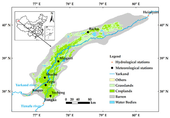
Figure 1.
Map of the Yarkand Oasis. The land cover type is from the data from 2017.
2.3. Data
The data used in this study included LAI, land cover, meteorological data (including precipitation, temperature, and relative humidity), runoff, and CO2 concentration, ranging from 2001 to 2017 (Table 1).

Table 1.
Summary of datasets for the research.
The moderate resolution imaging spectroradiometer (MODIS) LAI Collection 6 product MOD12A2H.006 [41] from 2001 to 2017 are used to quantitatively analyze the changes in vegetation LAI in the study area. Its spatial resolution is 500 m and temporal resolution is 8 days. The data of the MODIS land cover product MCD12Q2.006_LC_Type1 [42] from 2001 to 2017 are used to quantitatively analyze the land cover changes in the study area, which are classified according to the classification criteria of the International Geosphere–Biosphere Program (IGBP), with a temporal resolution of 1 year and a spatial resolution of 500 m. The precipitation, temperature, relative humidity, and wind speed data are from the China Meteorological Data Network (https://data.cma.cn), and they are the daily data from 2001 to 2017. The study area has a total of five meteorological stations, their locations were shown in Figure 1. The oasis is recharged by the Yarkand River and the Tiznafu River. The inflow stations are the Kaqun and Jiangka stations, and the downstream outflow is controlled by the Heiniyazi station (see Figure 1).
2.4. Data Processing
Regarding land cover, the ratio of the number of pixels representing vegetation types (i.e., open shrublands, grassland, croplands, and cropland/natural vegetation mosaics) to the total number of pixels in the region is denoted as Fveg. It is assumed that there is no seasonal change in land cover. Table 2 lists the average ratio of various land cover types in the region from 2001 to 2017.
Table 2.
The ratio of various land cover types in Yarkand Oasis from 2001 to 2017.
The regional average LAI (Lregion) could be estimated as the accumulated LAI value of vegetation pixels dividing by the total pixels number covering the study area. Then, the growing season was defined as the period from April to October [43], and the growing season mean LAI was calculated using the arithmetic average method according to MOD12A2H.006.
The vapor pressure deficit (v) was calculated using the following Equation [44]:
where AT (°C) is the atmospheric temperature at 2 m and RH (1%) is the relative humidity at 2 m. The Thiessen polygon method [45], which is a simple method to reflect the spatial variability, was used to calculate the regional average daily value from the daily v of each station in the Yarkand Oasis, and the arithmetic average method was used to calculate the growing season mean v according to daily v.
The total vegetation transpiration in vegetation area T (mm/year) could be calculated as:
where W (mm/year) represents the total water consumption in vegetation area and R ((mm/year)/(mm/year)) is the ratio of transpiration to evapotranspiration. In the study, the inter-annual variation of surface water storage is ignored since there is no over-year regulation reservoir in the Yarkand Oasis. The inter-annual variation of soil moisture was also ignored. Therefore, W was calculated as follows:
where I (mm/year) is the upstream surface inflow into the oasis, O (mm/year) is the downstream surface outflow from the oasis. I and O are obtained by dividing inflow and outflow runoff (m3/year), respectively, by vegetation area (m2) every year with an assumption that runoff is only consumed in vegetation region. P (mm/year) is the precipitation and ΔG (mm/year) is the groundwater variation. According to the research report [46], net ground flow only accounted for ~0.24% of the surface flow in the Yarkand Oasis. Therefore, net ground flow can be ignored in this analysis. The monthly precipitation, surface inflow, and surface outflow from 2001 to 2017 are given in Figure A1 in the Appendix A. Thus, the last part of W is groundwater variation (ΔG), which is calculated as follows:
where (mm/mm) represents the specific yield of groundwater, and as the study area is mainly covered by sandy soil, 0.1 m/m is used [47]. (mm/year) represents the variation in groundwater depth. Chen et al. [48] estimated a -18 m/year change in groundwater level from 1993 to 2011 based on 55 gauges across the oasis. Therefore, the value of is set to be 0.18 m/year for this study. The ratio R in Equation (12) is calculated based on Wei et al. [49] and Wang et al. [50]. According to Wei et al. [49],
where Rcrops and Rsg represent the T/ET of crops and shrubs/grasses, respectively, and then Lcrops and Lsg represent the LAI of crops and shrubs/grasses, respectively. According to Wang et al. [50]:
where Ras, Rns, and Rans represent the T/ET of the agricultural systems, natural system, and overall systems, respectively, and Las, Lns, and Lans represent the LAI of the agricultural system, natural system, and overall system, respectively. In the Yarkand Oasis, the vegetation types can be categorized into crops and shrubs/grasses, and they also can be categorized into agricultural system and natural system. Therefore, we took a simple way to estimate R during every growing season, i.e., calculating the five different ratios by using Equations (15)–(19) and replacing Lcrops, Lsg, Las, Lns, and Lans by L during every growing season, and then taking the arithmetic average of the five ratios as R. In addition, maximum and minimum of the five ratios are used to calculate maximum and minimum of T, which constitute the error limit of T.
The CO2 concentration (Ca) in this study area is assumed to be represented by that measured at the Waliguan Observatory, since both the Waliguan Observatory and Yarkand Oasis are located in the arid region of the Eurasian continent, and the distance between them is only approximately 2000 km. We could not obtain Ca of 2017, so it was obtained by interpolation using the Ca of the Hawaii Observatory, since there was a high correlation of Ca at the Waliguan Observatory and Hawaii Observatory, with the R2 of the linear regression up to 0.989 from 2001 to 2016 (Figure A2). Then, the growing season mean Ca were calculated as the arithmetic mean of the daily CO2 concentration during the growing season.
2.5. Calculation of Change Rate
To estimate the changes of variables, the Mann–Kendall method was used to test the trend of a given time series [51,52], and then the linear regression method was used to obtain the trend line of the time series [53]. Finally, the interannual change of variables was calculated as:
where represents the interannual change of a variable (%/year), , , and represent the end value, initial value, and average value, respectively, of the trend line, and n represents the time series length. Finally, , , , , and were calculated using Equation (20).
3. Results
3.1. Changes in Vegetation and Environmental Variables
Figure 2 shows the changes in LAI, mean vapor pressure deficit, mean CO2 concentration, cumulative transpiration per vegetation area, and mean wind speed during the growing season, together with the ratio of vegetation area from 2001 to 2017 in the Yarkand Oasis. The growing season mean LAI of the oasis increased significantly (p < 0.001), from 0.268 m2/m2 in 2001 to 0.370 m2/m2 in 2017, with an annual growth rate of 2.31%/year. The growing season accumulative vegetation transpiration changed with a low significant level (p = 0.3252), and could be considered constant, which was consistent with the assumption of Donohue et al. [10]. The growing season mean vapor pressure deficit had a significant increasing trend from 2001 to 2017 (p < 0.05), with an annual growth rate of 0.80%/year. Fveg also increased significantly (p < 0.001), from 41.9% in 2001 to 47.9% in 2017, with an annual growth rate of 1.06%/year. According to the data from the Waliguan Observatory, the growing season mean CO2 concentration increased significantly (p < 0.001), from 370 ppm in 2001 to 407 ppm in 2017, with an annual growth rate of 0.56%/year.
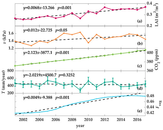
Figure 2.
Interannual changes in (a) the oasis-averaged growing season leaf area index (Lregion, m2/m2), (b) growing season mean vapor pressure deficit (v, kPa), (c) growing season mean atmospheric carbon dioxide concentration (Ca, ppm), (d) growing season accumulative transpiration (T, mm/year), and (e) the ratio of vegetation area to oasis area (Fveg) over the period 2001–2017 for Yarkand Oasis. T was estimated from water consumption per vegetation area by multiplying the ratio of vegetation transpiration to regional evaporation, which was calculated according to Equations (15)–(19) and the maximum and minimum of estimated T were shown as the error bars in subplot (d).
3.2. Attribution of Vegetation Change
Table 3 shows the annual average rate of change in variables in the Yarkand Oasis. The simulated LAI change by using Equation (10) was 1.20%/year. The relative contribution rate of each factor is shown in Figure 3. Among all the factors, change in vegetation cover ratio due to LULCC had the largest contribution (88.33%). The unchanged transpiration had no impact on vegetation change (0.0%), which indirectly reflects the impact of water availability per vegetation area. In addition, the contributions from enhancing CO2 concentration and increasing vapor pressure deficit were 40.0% and -28.3%, respectively. They had approximate values in magnitude but opposite signs. From the perspective of vegetation WUE, the facilitation of elevated-CO2 was greater than the inhibition of elevated-v, thus improving the WUE.
Table 3.
The observed and simulated leaf area index (LAI) in Yarkand Oasis and its causes, together with the relative contribution rate of each cause. is the change rate of LAI, together with the observed and simulated indicating the observed from moderate resolution imaging spectroradiometer (MODIS) and the simulated using the improved Donohue13 model, respectively. , , , and denote the impacts from changes in transpiration, CO2 concentration, vapor pressure deficit, and land use and land cover, respectively.
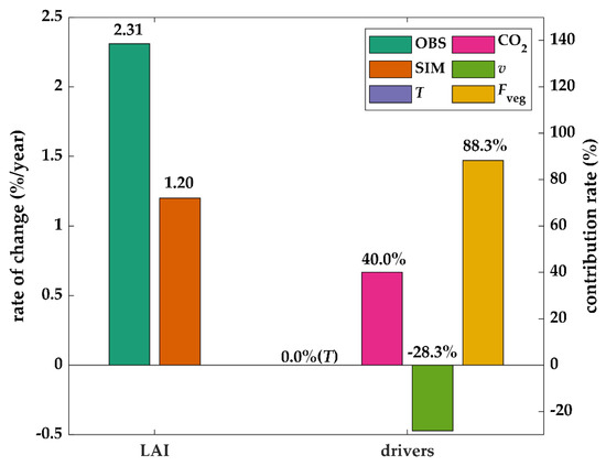
Figure 3.
The change rates of satellite-observed LAI (OBS) and simulated LAI (SIM) and the contributions from changes in transpiration (T), carbon dioxide concentration (CO2), water vapor pressure difference (v), and the ratio of vegetation area to oasis area (Fveg) over the period 2001–2017 for Yarkand Oasis.
4. Discussion
4.1. Applicability of the Improved Donohue13 Model
This study detected a 2.31%/year greening trend in the growing-season of the Yarkand Oasis from 2001 to 2017, which was consistent with the previous studies [24,54,55]. However, the simulated greening trend was 1.21%/year and approximately accounted for half of the observed trend. The difference between the simulated and observed trend might be caused by the following two reasons:
- 1)
- Data error: According to the evaluation of Yan et al. [56], MODIS LAI Product Collection 6 was underestimated in grassland and cropland, which causes an overestimation of trend by Equation (22) due to underestimation of and constant of in Equation (22). Furthermore, the change in vapor pressure deficit (v) might be overestimated. On one hand, these meteorological stations are located in urban areas, resulting in a stronger upward trend than vegetation areas in v [57]. On the other hand, Bachu and Yecheng, which are closed to the desert and represent inadequate water supply condition, had weaker upward trends of v than regional mean v. While Maigaiti, Shache, and Zepu, located inside the oasis with an abundant water supply condition, had stronger increase trends of v (Table 4). Actually, Yarkand Oasis is located on the edge of Taklimakan Desert, and vegetation might be under inadequate water supply condition. Therefore, change in v of Bachu and Yecheng might be closer to represent the actual change in v of Yarkand Oasis. In a word, the change in v might be overestimated, which amplifies the inhibition of v on vegetation growth.
Table 4. Changes in v and their significant level in five meteorological stations of Yarkand oasis.
- 2)
- Seed optimization: Cropland was one of the main land cover type in Yarkand Oasis, accounting for 20.4% of the total oasis area in 2001–2017 (Table 2). As agricultural science advances, crop seeds were continuously improved. Optimized seeds may increase water use efficiency (WUE) by themselves, which causes a lower Ci/Ca and furthermore a greater d(1 − Ci/Ca)/(1 − Ci/Ca) [58]. Removing the simplification that (1 − Ci/Ca) was proportional to , Equation (12) can be rewritten as:
Therefore, a greater d(1 − Ci/Ca)/(1 − Ci/Ca) due to seed optimization might cause a greater value of simulated .
In Equation (10), the transpiration T implies the effect of water availability in the vegetation area, which had no impact on vegetation change in the Yarkand Oasis (0.0%). To calculate the vegetation transpiration per vegetation area (T), five empirical formulas, i.e., Equations (15)–(19), were used in this study. As shown in Table 5, the significance levels of change in T based on different T estimated Equations (15)–(19) were greater than 0.2, which indicates unchanged T. Therefore, it means that the uncertainty due to different formula for T could be acceptable. Moreover, Equations (15)–(19) focus on the partition of evapotranspiration between soil evaporation and transpiration. Besides, the water consumption includes water surface evaporation. However, in the Yarkand Oasis, water surface covers ~0.6% area, which possibly led to a relatively small error in the calculated T. In addition, the impacts of anthropogenic activities, such as the optimization of irrigation methods, were not considered in our study. The optimization irrigation methods might decrease soil evaporation (E) of cropland and increase estimated transpiration (T). The increase in the T of cultivated land might affect the change of total T of the oasis, which needs further studying in the future.
Table 5.
The significant levels of change in transpiration (T) based on different T estimated Equations (15)–(19).
The results show that the facilitation of the increase in WUE to LAI was 11.7% (0.14%/year), as calculated as = 40.0% (0.48%/year) − 28.3% (0.34%/year). It was similar to the FACE experiments, which show that an elevated CO2 concentration may increase the WUE of vegetation and further promotes vegetation [59,60,61,62]. In addition, coefficient of k in Equation (11) was assumed to relate to species and was assigned 0.5 by default. In order to analyze the impact of different species, the values of 0.4, 0.5, and 0.6 were set, which reflected the effectiveness of different species on resource availability. As shown in Table 6, there were small differences in the contribution analysis caused by different coefficients of k. It indicates that the results were not sensitive to species.
Table 6.
The contribution analysis based on a different coefficient of k in Equation (11). , , and denote the contribution rate of CO2 concentration, vapor pressure deficit, and the difference between the two, respectively.
Furthermore, to evaluate the applicability of the improved model to different land cover type, the results in grassland and cropland, respectively, were presented with the assumption that transpiration per grassland or cropland area was constant. As shown in Table 7, there were small differences between observed and simulated changes in Lgrass, indicating a good performance in grassland. In contrast, as shown in Table 8, the result in cropland was relatively poor with a difference of 0.97%/year between observed and simulated Lcrop, which might be caused by data error and seed optimization.
Table 7.
The observed and simulated LAI in the grassland of Yarkand Oasis and its causes (unit: %/year). is the change rate of LAI in grassland, together with the observed and simulated indicating the observed from MODIS and the simulated using the improved Donohue13 model, respectively. , , , and denote the impacts from changes in transpiration, CO2 concentration, vapor pressure deficit, and ratio of grassland area, respectively.
Table 8.
The observed and simulated LAI in cropland of Yarkand Oasis and its causes (unit: %/year). is the change rate of LAI in cropland, together with the observed and simulated indicating the observed from MODIS and the simulated using the improved Donohue13 model, respectively. , , , and denote the impacts from changes in transpiration, CO2 concentration, vapor pressure deficit, and ratio of cropland area, respectively.
4.2. Impact of Water Availability
The observed unchanged transpiration in vegetation area verifies the assumption that water consumption per vegetation area is constant in arid regions [12]. For a specific species, transpiration consumption for growth could be considered constant. In such arid regions, the water availability per vegetation area almost only makes up for the lack of vegetation transpiration for growth and accompanying soil evaporation during the growing season, and does not have too much excess during the growing season or water storage in the non-growing season. Therefore, water determines vegetation, but vegetation does not determine how much water to consume.
Although the water availability per vegetation area was constant, the total water availability was actually increasing. As shown in results, the vegetation area ratio (Fveg) was increasing, which was probably driven by increased total water availability. In other words, more Fveg could be fed by more total water availability with constant transpiration consumption per vegetation area. Furthermore, the water availability mainly originated from local precipitation and inflow from outside. In the region that precipitation dominates the water availability, precipitation has a determining influence on vegetation [63,64,65]. In the region that most water availability comes from outside, such as the Yarkand Oasis, the water is mainly supplied by the streamflow from glacier and snow melting and plays a dominant role in vegetation change, and this pattern of water supply and consumption is widespread in Central Asia [66,67]. Due to global warming, the water from glaciers and snowmelt in Central Asia has increased significantly [68,69,70,71], and it increases the total water availability in the region [72,73]. Thus it plays an important role in the regional vegetation greening [74]. However, a decrease in total water availability may be expected by the end of the twenty-first century as a result of depleted glaciers without refreezing [75,76], which means that the vegetation greening due to Fveg driven by increased total water availability is unsustainable.
4.3. Impact of LULCC Change
Using the improved Donohue13 model, we found that the change of LULCC contributes the most (88.3%) to the LAI change in the Yarkand Oasis, which is consistent with the results of Wang et al. [17] in the arid region of the Heihe River basin. Similarly, a number of studies on vegetation change in the Sahel region showed that LULCC plays an important role [28,29,77]. In recent years, some large-scale studies on the attribution analysis of vegetation change have begun to consider the impact of LULCC after recognizing its possible important role [9,10]. However, due to factors such as the uncertainty of the model and coarse spatial resolution, those studies may have large uncertainty in assessing the role of LULCC. For example, Zhu et al. [10] estimated the contribution of LULCC to global greening (4%) but the results from different ecological models had significant differences in magnitude and even in signs ranging from -11% to 18.4%. Furthermore, in their study, the spatial resolution was coarse (0.5°), which made it difficult to fully reflect the change in LULCC. Therefore, it is possible that they underestimated the contribution of LULCC to global greening. The improved Donohue13 model provides a simple but feasible tool to re-evaluate the impact role of LULCC on global greening based on finer land use map.
4.4. Implication of Improved Donohue13 Model
It is a hot topic to study the vegetation response to changing environments, including climate change, elevated atmospheric CO2 concentration, and anthropogenic activities. In previous studies, the commonly used methods are statistical analysis [54,78,79] and process-based model simulation [9,10,21,80]. Generally speaking, the statistical analysis is difficult to quantify; while the process-based model has uncertainties in input data, structure, and parameters, and at the same time, it cannot provide an intuitive way to reveal the relationship of vegetation change with environmental factors. The improved Donohue13 model is physical-based and its variable relationship is explicit, which may be used to explore the relationship of vegetation change with environmental factors.
The interaction of vegetation and hydrology forms a coupled vegetation-hydrological system, changed by climate change, elevated CO2 concentration, and anthropogenic activities, which causes changes in regional hydrological processes and water resource [5,81]. In previous studies, the watershed coupled water-energy balance equation (i.e., Budyko framework) relates evapotranspiration (E) with precipitation (P) and potential evapotranspiration (E0) [82], and the equation includes a unique empirical parameter (n) related to vegetation [83]. Under the Budyko framework, many studies have analyzed the response of runoff to changing environment [84,85], yet based on the assumption that n is constant. In fact, the parameter n is changing with changing environment, and one of its main drivers is vegetation for a particular catchment [86], with a relationship of between n and LAI [87]. Moreover, the improved Donohue13 model can explicitly express the relationship between vegetation change and environmental variables on the catchment scale and provide a method to estimate the change in n. Therefore, it is a possible way for investigating the response of coupled vegetation-hydrology systems under environment change to couple the improved Donohue13 model and the Budyko framework.
5. Conclusions
Vegetation shows a greening trend on the global scale in the past decades, which has an important effect on hydrological cycle. At the same time, many studies have shown that LULCC plays an important role in vegetation change. To quantitatively interpret causes for vegetation greening, this study improved the Donohue13 model by taking into account the change in ratio of vegetation coverage area to total regional area due to LULCC, furthermore applies this model to the Yarkand Oasis in the arid region of northwest China. The results show that the regional mean LAI during the growing season significantly increased at a rate of 2.31%/year from 2001 to 2017. Due to data error and seed optimization, there is not good performance of the improved Donohue13 model with a 1.20%/yr upward trend. On the vegetation greening in the Yarkand Oasis, the contributions of: (1) LULCC; (2) atmospheric CO2 concentration; and (3) vapor pressure deficit were: (1) 88.3%; (2) 40.0%; and (3) -28.3%. It means that the greatest contribution was from LULCC, which is probably driven by increased total water availability in the whole oasis with constant transpiration in the vegetation area. The improved Donohue13 model, a simple but physics-based model, can help explain the impact of climate change and anthropogenic activity variables on vegetation change in arid regions. It can be further combined with the Budyko hypothesis to establish a framework for quantifying the changes in coupled response of vegetation and hydrological processes to environment changes.
Author Contributions
Conceptualization, X.Y. and H.Y.; Data curation, X.Y. and H.Y.; Formal analysis, X.Y.; Funding acquisition, H.Y.; Investigation, X.Y.; Methodology, X.Y. and H.Y.; Resources, H.Y. and D.Y.; Supervision, H.Y.; Validation, X.Y., H.Y. and S.L.; Writing—original draft, X.Y.; Writing—review & editing, X.Y. and H.Y.
Funding
This research was partially supported by funding from the National Natural Science Foundation of China (Grant Nos. 51622903, 51622907, and 51979140), the National Program for Support of Top-notch Young Professionals, and the Program from the State Key Laboratory of Hydro-Science and Engineering of China (Grant No. 2017-KY-01). And the APC was funding by the National Natural Science Foundation of China (Grant No. 51622903).
Acknowledgments
We would like to thank the three anonymous reviewers for their constructive comments and language editing.
Conflicts of Interest
The authors declare no conflict of interest.
Appendix A
Figure A1 shows that the monthly precipitation (P), surface inflow (I), and surface outflow (O) in vegetation area of Yarkand Oasis from 2001 to 2017. The monthly P can be estimated as the sum of the daily P, which is calculated from daily P of meteorological stations in the Yarkand Oasis using the Thiessen polygon method, during each month. The monthly I and O are obtained by the monthly inflow at the Kaqun and Jiangka stations and the monthly outflow at the Heiniyazi station, respectively.

Figure A1.
The monthly precipitation (P), surface inflow (I), and surface outflow (O) in vegetation area of Yarkand Oasis from 2001 to 2017.
Figure A2 shows that the square of correlation coefficient (R2) of the linear regression of growing season mean atmospheric CO2 concentration (Ca) between the Hawaii Observatory and Wanliguan Observatory from 2001 to 2016.

Figure A2.
The correlation of the growing season mean CO2 concentrations at the Hawaii and Waliguan Observatories from 2001 to 2016.
References
- Wang, X.; Piao, S.; Ciais, P.; Li, J.; Friedlingstein, P.; Koven, C.; Chen, A. Spring temperature change and its implication in the change of vegetation growth in North America from 1982 to 2006. Proc. Natl. Acad. Sci. USA 2011, 108, 1240–1245. [Google Scholar] [CrossRef] [PubMed]
- Nemani, R.R.; Keeling, C.D.; Hashimoto, H.; Jolly, W.M.; Piper, S.C.; Tucker, C.J.; Myneni, R.B.; Running, S.W. Climate-driven increases in global terrestrial net primary production from 1982 to 1999. Science 2003, 300, 1560–1563. [Google Scholar] [CrossRef] [PubMed]
- Parmesan, C.; Yohe, G. A globally coherent fingerprint of climate change impacts across natural systems. Nature 2003, 421, 37–42. [Google Scholar] [CrossRef] [PubMed]
- Xu, L.; Myneni, R.B.; Chapin, F.S., III; Callaghan, T.V.; Pinzon, J.E.; Tucker, C.J.; Zhu, Z.; Bi, J.; Ciais, P.; Tømmervik, H.; et al. Temperature and vegetation seasonality diminishment over northern lands. Nat. Clim. Chang. 2013, 3, 581–586. [Google Scholar] [CrossRef]
- Yang, D.; Lei, H.; Cong, Z. Overview of the research status in interaction between hydrological processes and vegetation in catchment (in Chinese). Shuili Xuebao(J. Hydraul. Eng.) 2010, 41, 1142–1149. [Google Scholar]
- Piao, S.; Friedlingstein, P.; Ciais, P.; Zhou, L.; Chen, A. Effect of climate and CO2 changes on the greening of the Northern Hemisphere over the past two decades. Geophys. Res. Lett. 2006, 33. [Google Scholar] [CrossRef]
- Los, S.O. Analysis of trends in fused AVHRR and MODIS NDVI data for 1982-2006: Indication for a CO2 fertilization effect in global vegetation. Glob. Biogeochem. Cycle 2013, 27, 318–330. [Google Scholar] [CrossRef]
- Lucht, W.; Prentice, I.C.; Myneni, R.B.; Sitch, S.; Friedlingstein, P.; Cramer, W.; Bousquet, P.; Buermann, W.; Smith, B. Climatic control of the high-latitude vegetation greening trend and Pinatubo effect. Science 2002, 296, 1687–1689. [Google Scholar] [CrossRef]
- Mao, J.; Shi, X.; Thornton, P.; Hoffman, F.; Zhu, Z.; Myneni, R. Global Latitudinal-Asymmetric Vegetation Growth Trends and Their Driving Mechanisms: 1982–2009. Remote Sens. Basel. 2013, 5, 1484–1497. [Google Scholar] [CrossRef]
- Zhu, Z.; Piao, S.; Myneni, R.B.; Huang, M.; Zeng, Z.; Canadell, J.G.; Ciais, P.; Sitch, S.; Friedlingstein, P.; Arneth, A.; et al. Greening of the Earth and its drivers. Nat. Clim. Chang. 2016, 6, 791–795. [Google Scholar] [CrossRef]
- Beck, H.E.; McVicar, T.R.; van Dijk, A.I.J.M.; Schellekens, J.; de Jeu, R.A.M.; Bruijnzeel, L.A. Global evaluation of four AVHRR–NDVI data sets: Intercomparison and assessment against Landsat imagery. Remote Sens. Environ. 2011, 115, 2547–2563. [Google Scholar] [CrossRef]
- Donohue, R.J.; Roderick, M.L.; McVicar, T.R.; Farquhar, G.D. Impact of CO2 fertilization on maximum foliage cover across the globe’s warm, arid environments. Geophys. Res. Lett. 2013, 40, 3031–3035. [Google Scholar] [CrossRef]
- Donohue, R.J.; Mcvicar, T.R.; Roderick, M.L. Climate-related trends in Australian vegetation cover as inferred from satellite observations, 1981–2006. Glob. Chang. Biol. 2009, 15, 1025–1039. [Google Scholar] [CrossRef]
- Goetz, S.J.; Bunn, A.G.; Fiske, G.J.; Houghton, R.A.; Woodwell, G.M. Satellite-Observed Photosynthetic Trends across Boreal North America Associated with Climate and Fire Disturbance. Proc. Natl. Acad. Sci. USA 2005, 102, 13521–13525. [Google Scholar] [CrossRef] [PubMed]
- Shen, Q.; Gao, G.; Han, F.; Xiao, F.; Ma, Y.; Wang, S.; Fu, B. Quantifying the effects of human activities and climate variability on vegetation cover change in a hyper-arid endorheic basin. Land Degrad. Dev. 2018, 29, 3294–3304. [Google Scholar] [CrossRef]
- Malhi, Y.; Roberts, J.T.; Betts, R.A.; Killeen, T.J.; Li, W.; Nobre, C.A. Climate change, deforestation, and the fate of the Amazon. Science 2008, 319, 169–172. [Google Scholar] [CrossRef] [PubMed]
- Wang, Y.; Roderick, M.L.; Shen, Y.; Sun, F. Attribution of satellite-observed vegetation trends in a hyper-arid region of the Heihe River basin, Western China. Hydrol. Earth Syst. Sci. 2014, 18, 3499–3509. [Google Scholar] [CrossRef]
- Reich, P.B.; Hobbie, S.E.; Lee, T.D. Plant growth enhancement by elevated CO2 eliminated by joint water and nitrogen limitation. Nat. Geosci. 2014, 7, 920–924. [Google Scholar] [CrossRef]
- Lu, X.; Wang, L.; McCabe, M.F. Elevated CO2 as a driver of global dryland greening. Sci. Rep.-UK 2016, 6, 2045–2322. [Google Scholar] [CrossRef] [PubMed]
- Reich, P.B.; Hobbie, S.E. Decade-long soil nitrogen constraint on the CO2 fertilization of plant biomass. Nat. Clim. Chang. 2013, 3, 278–282. [Google Scholar] [CrossRef]
- Piao, S.; Yin, G.; Tan, J.; Cheng, L.; Huang, M.; Li, Y.; Liu, R.; Mao, J.; Myneni, R.B.; Peng, S.; et al. Detection and attribution of vegetation greening trend in China over the last 30 years. Glob. Change Biol. 2015, 21, 1601–1609. [Google Scholar] [CrossRef] [PubMed]
- Zeng, B.; Yang, T. Impacts of climate warming on vegetation in Qaidam Area from 1990 to 2003. Environ. Monit. Assess. 2008, 144, 403–417. [Google Scholar] [CrossRef] [PubMed]
- Roerink, G.J.; Menenti, M.; Soepboer, W.; Su, Z. Assessment of climate impact on vegetation dynamics by using remote sensing. Phys. Chem. Earth Parts A/B/C 2003, 28, 103–109. [Google Scholar] [CrossRef]
- Wang, Y.; Shen, Y.; Chen, Y.; Guo, Y. Vegetation dynamics and their response to hydroclimatic factors in the Tarim River Basin, China. Ecohydrology 2013, 6, 927–936. [Google Scholar] [CrossRef]
- Zhang, X.; Goldberg, M.; Tarpley, D.; Friedl, M.A.; Morisette, J.; Kogan, F.; Yu, Y. Drought-induced vegetation stress in southwestern North America. Environ. Res. Lett. 2010, 5, 24008. [Google Scholar] [CrossRef]
- Fensholt, R.; Langanke, T.; Rasmussen, K.; Reenberg, A.; Prince, S.D.; Tucker, C.; Scholes, R.J.; Le, Q.B.; Bondeau, A.; Eastman, R.; et al. Greenness in semi-arid areas across the globe 1981–2007—An Earth Observing Satellite based analysis of trends and drivers. Remote Sens. Environ. 2012, 121, 144–158. [Google Scholar] [CrossRef]
- Dardel, C.; Kergoat, L.; Hiernaux, P.; Mougin, E.; Grippa, M.; Tucker, C.J. Re-greening Sahel: 30years of remote sensing data and field observations (Mali, Niger). Remote Sens. Environ. 2014, 140, 350–364. [Google Scholar] [CrossRef]
- Bégué, A.; Vintrou, E.; Ruelland, D.; Claden, M.; Dessay, N. Can a 25-year trend in Soudano-Sahelian vegetation dynamics be interpreted in terms of land use change? A remote sensing approach. Glob. Environ. Chang. 2011, 21, 413–420. [Google Scholar] [CrossRef]
- Brandt, M.; Verger, A.; Diouf, A.; Baret, F.; Samimi, C. Local Vegetation Trends in the Sahel of Mali and Senegal Using Long Time Series FAPAR Satellite Products and Field Measurement (1982–2010). Remote Sens.-Basel 2014, 6, 2408–2434. [Google Scholar] [CrossRef]
- Wong, S.C.; Cowan, I.R.; Farquhar, G.D. Stomatal conductance correlates with photosynthetic capacity. Nature 1979, 282, 424–426. [Google Scholar] [CrossRef]
- Wong, S.; Dunin, F. Photosynthesis and Transpiration of Trees in a Eucalypt Forest Stand: C02, Light and Humidity Responses. Funct. Plant Biol. 1987, 14, 619–632. [Google Scholar] [CrossRef]
- Farquhar, G.D.; Lloyd, J.; Taylor, J.A.; Flanagan, L.B.; Syvertsen, J.P.; Hubick, K.T.; Wong, S.C.; Ehleringer, J.R. Vegetation effects on the isotope composition of oxygen in atmospheric C02. Nature 1993, 363, 439–443. [Google Scholar] [CrossRef]
- Medlyn, B.E.; Duursma, R.A.; Eamus, D.; Ellsworth, D.S.; Prentice, I.C.; Barton, C.V.M.; Crous, K.Y.; De Angelis, P.; Freeman, M.; Wingate, L. Reconciling the optimal and empirical approaches to modelling stomatal conductance. Glob. Chang. Biol. 2011, 17, 2134–2144. [Google Scholar] [CrossRef]
- Lu, H. Decomposition of vegetation cover into woody and herbaceous components using AVHRR NDVI time series. Remote Sens. Environ. 2003, 86, 1–18. [Google Scholar] [CrossRef]
- Donohue, R.J.; Roderick, M.L.; McVicar, T.R.; Yang, Y. A simple hypothesis of how leaf and canopy-level transpiration and assimilation respond to elevated CO2 reveals distinct response patterns between disturbed and undisturbed vegetation. J. Geophys. Res. Biogeosci. 2017, 122, 168–184. [Google Scholar] [CrossRef]
- Friedlingstein, P.; Joel, G.; Field, C.B.; Fung, I.Y. Toward an allocation scheme for global terrestrial carbon models. Glob. Chang. Biol. 1999, 5, 755–770. [Google Scholar] [CrossRef]
- Dilbar, A.; Hamit, Y.; WANG, Z. The Relationship Between Oases and Water Resources in Tarim Basin. J. Xinjiang Univ. (Nat. Sci. Ed.) (Chin.) 2006, 23, 216–218. [Google Scholar]
- Ren, J.; Wu, Q. Study on Dynamic Variation of Water-salt in Salinized Irrigation Area of Xinjiang Yerqiang River. J. Shandong Univ. Sci. Technol. (Chin.) 2009, 28, 8–12. [Google Scholar]
- Li, X.; Yang, K.; Zhou, Y. Progress in the study of oasis-desert interactions. Agric. For. Meteorol. 2016, 230–231, 1–7. [Google Scholar] [CrossRef]
- Xu, J.; Chen, Y.; Li, W.; Nie, Q.; Hong, Y.; Yang, Y. The nonlinear hydro-climatic process in the Yarkand River, northwestern China. Stoch. Environ. Res. Risk Assess. 2013, 27, 389–399. [Google Scholar] [CrossRef]
- Myneni, R.; Knyazikhin, Y.; T, P. MOD15A2H MODIS/Terra Leaf Area Index/FPAR 8-Day L4 Global 500m SIN Grid V006 [Data set]; NASA EOSDIS Land Processes DAAC: Sioux Falls, SD, USA, 2015. [Google Scholar]
- Friedl, M.; Gray, J.; Sulla-Menashe, D. MCD12Q2 MODIS/Terra+Aqua Land Cover Dynamics Yearly L3 Global 500m SIN Grid V006 [Data set]; NASA EOSDIS Land Processes DAAC: Sioux Falls, SD, USA, 2019. [Google Scholar]
- Piao, S.; Mohammat, A.; Fang, J.; Cai, Q.; Feng, J. NDVI-based increase in growth of temperate grasslands and its responses to climate changes in China. Global Environ. Chang. 2006, 16, 340–348. [Google Scholar] [CrossRef]
- Allen, R.G.; Pereira, L.S.; Raes, D.; Smith, M. Crop Evapotranspiration—Guidelines for Computing Crop Water Requirements-FAO Irrigation and Drainage Paper 56; FAO: Rome, Italy, 1998; p. 300. [Google Scholar]
- Rhynsburger, D. Analytic delineation of Thiessen polygons. Geogr. Anal. 1973, 5, 133–144. [Google Scholar] [CrossRef]
- Lei, Z.; Yang, S.; Cong, Z.; Ni, G.; Yang, H.; Huang, Y.; Liu, Z.; Yang, H.; Li, P.; Li, Z.; et al. Research Report on Water Consumption in Yarkand Oasis (in Chinese); Department of Hydraulic Engineering, Tsinghua University: Beijing, China, 2006. [Google Scholar]
- Johnson, A.I. Specific yield: Compilation of specific yields for various materials. In Water Supply Paper; US Government Printing Office: Washington, DC, USA, 1967. [Google Scholar]
- Chen, Z.; Yang, H.; Chen, D. Analysis of groundwater table depth changes in Yarkant plain oasis in recent 20 years and their causes. J. Hydroelectr. Eng. (Chin.) 2016, 35, 58–66. [Google Scholar]
- Wei, Z.; Yoshimura, K.; Wang, L.; Miralles, D.G.; Jasechko, S.; Lee, X. Revisiting the contribution of transpiration to global terrestrial evapotranspiration. Geophys. Res. Lett. 2017, 44, 2792–2801. [Google Scholar] [CrossRef]
- Wang, L.; Good, S.P.; Caylor, K.K. Global synthesis of vegetation control on evapotranspiration partitioning. Geophys. Res. Lett. 2014, 41, 6753–6757. [Google Scholar] [CrossRef]
- Kendall, M.G. Rank Correlation Methods; Griffin: London, UK, 1975. [Google Scholar]
- Mann, H. Nonparametric tests against trend. Econometr. J. Econometr. Soc. 1945, 13, 245–259. [Google Scholar] [CrossRef]
- Seber, G.A.; Lee, A.J. Linear Regression Analysis; John Wiley & Sons: Hoboken, NJ, USA, 2012; Volume 329. [Google Scholar]
- Guli, J.; Liang, S.; Yi, Q.; Liu, J. Vegetation dynamics and responses to recent climate change in Xinjiang using leaf area index as an indicator. Ecol. Indic. 2015, 58, 64–76. [Google Scholar]
- Zhao, X.; Tan, K.; Zhao, S.; Fang, J. Changing climate affects vegetation growth in the arid region of the northwestern China. J. Arid Environ. 2011, 75, 946–952. [Google Scholar] [CrossRef]
- Yan, K.; Park, T.; Yan, G.; Liu, Z.; Yang, B.; Chen, C.; Nemani, R.; Knyazikhin, Y.; Myneni, R. Evaluation of MODIS LAI/FPAR Product Collection 6. Part 2: Validation and Intercomparison. Remote Sens.-Basel 2016, 8, 460. [Google Scholar] [CrossRef]
- Luo, M.; Lau, N.C. Urban expansion and drying climate in an urban agglomeration of east China. Geophys. Res. Lett. 2019. [Google Scholar] [CrossRef]
- Tong, X.; Li, J.; Yu, Q.; Qin, Z. Ecosystem water use efficiency in an irrigated cropland in the North China Plain. J. Hydrol. 2009, 374, 329–337. [Google Scholar] [CrossRef]
- Norby, R.J.; DeLucia, E.H.; Gielen, B.; Calfapietra, C.; Giardina, C.P.; King, J.S.; Ledford, J.; McCarthy, H.R.; David, J.P.M.; Ceulemans, R.; et al. Forest response to elevated CO2 is conserved across a broad range of productivity. Proc. Natl. Acad. Sci. USA 2005, 102, 18052–18056. [Google Scholar] [CrossRef]
- Norby, R.J.; Zak, D.R. Ecological Lessons from Free-Air CO2 Enrichment (FACE) Experiments. Annu. Rev. Ecol. Evol. Syst. 2011, 42, 181–203. [Google Scholar] [CrossRef]
- O’Leary, G.J.; Christy, B.; Nuttall, J.; Huth, N.; Cammarano, D.; Stöckle, C.; Basso, B.; Shcherbak, I.; Fitzgerald, G.; Luo, Q.; et al. Response of wheat growth, grain yield and water use to elevated CO2 under a Free-Air CO2 Enrichment (FACE) experiment and modelling in a semi-arid environment. Global Chang. Biol. 2015, 21, 2670–2686. [Google Scholar] [CrossRef] [PubMed]
- Yoshimoto, M.; Oue, H.; Kobayashi, K. Energy balance and water use efficiency of rice canopies under free-air CO2 enrichment. Agric. For. Meteorol. 2005, 133, 226–246. [Google Scholar] [CrossRef]
- Shen, M.; Piao, S.; Cong, N.; Zhang, G.; Jassens, I.A. Precipitation impacts on vegetation spring phenology on the Tibetan Plateau. Glob. Chang. Biol. 2015, 21, 3647–3656. [Google Scholar] [CrossRef]
- Mariano, D.A.; Santos, C.A.C.D.; Wardlow, B.D.; Anderson, M.C.; Schiltmeyer, A.V.; Tadesse, T.; Svoboda, M.D. Use of remote sensing indicators to assess effects of drought and human-induced land degradation on ecosystem health in Northeastern Brazil. Remote Sens. Environ. 2018, 213, 129–143. [Google Scholar] [CrossRef]
- Xu, L.; Samanta, A.; Costa, M.H.; Ganguly, S.; Nemani, R.R.; Myneni, R.B. Widespread decline in greenness of Amazonian vegetation due to the 2010 drought. Geophys. Res. Lett. 2011, 38, 581–586. [Google Scholar] [CrossRef]
- Olsson, O.; Gassmann, M.; Wegerich, K.; Bauer, M. Identification of the effective water availability from streamflows in the Zerafshan river basin, Central Asia. J. Hydrol. 2010, 390, 190–197. [Google Scholar] [CrossRef]
- Duethmann, D.; Bolch, T.; Farinotti, D.; Kriegel, D.; Vorogushyn, S.; Merz, B.; Pieczonka, T.; Jiang, T.; Su, B.; Güntner, A. Attribution of streamflow trends in snow and glacier melt-dominated catchments of the Tarim River, Central Asia. Water Resour. Res. 2015, 51, 4727–4750. [Google Scholar] [CrossRef]
- Wang, X.; Luo, Y.; Sun, L.; He, C.; Zhang, Y.; Liu, S. Attribution of Runoff Decline in the Amu Darya River in Central Asia during 1951–2007. J. Hydrometeorol. 2016, 17, 1543–1560. [Google Scholar] [CrossRef]
- Casassa, G.; López, P.; Pouyaud, B.; Escobar, F. Detection of changes in glacial run-off in alpine basins: examples from North America, the Alps, central Asia and the Andes. Hydrol. Process. 2009, 23, 31–41. [Google Scholar] [CrossRef]
- Gan, R.; Luo, Y.; Zuo, Q.; Sun, L. Effects of projected climate change on the glacier and runoff generation in the Naryn River Basin, Central Asia. J. Hydrol. 2015, 523, 240–251. [Google Scholar] [CrossRef]
- Ye, B.; Yang, D.; Jiao, K.; Han, T.; Jin, Z.; Yang, H.; Li, Z. The Urumqi River source Glacier No. 1, Tianshan, China: Changes over the past 45 years. Geophys. Res. Lett. 2005, 32. [Google Scholar] [CrossRef]
- Gries, D.; Foetzki, A.; Arndt, S.K.; Bruelheide, H.; Thomas, F.M.; Zhang, X.; Runge, M. Production of Perennial Vegetation in an Oasis-desert Transition Zone in NW China - Allometric Estimation, and Assessment of Flooding and Use Effects. Plant. Ecol. 2005, 181, 23–43. [Google Scholar] [CrossRef]
- Lei, Z.D.; Hu, H.P.; Yang, S.X.; Tian, F.Q. Analysis on water consumption in oases of the Tarim Basin. J. Hydraul. Eng. (Chin.) 2006, 37, 1470–1475. [Google Scholar]
- Zhang, R.; Ouyang, Z.; Xie, X.; Guo, H.; Tan, D.; Xiao, X.; Qi, J.; Zhao, B. Impact of Climate Change on Vegetation Growth in Arid Northwest of China from 1982 to 2011. Remote Sens.-Basel 2016, 8, 364. [Google Scholar] [CrossRef]
- Bliss, A.; Hock, R.; Radić, V. Global response of glacier runoff to twenty-first century climate change. J. Geophys.l Res. Earth Surf. 2014, 119, 717–730. [Google Scholar] [CrossRef]
- Sorg, A.; Bolch, T.; Stoffel, M.; Solomina, O.; Beniston, M. Climate change impacts on glaciers and runoff in Tien Shan (Central Asia). Nat. Clim. Chang. 2012, 2, 725–731. [Google Scholar] [CrossRef]
- Wessels, K.J.; Prince, S.D.; Malherbe, J.; Small, J.; Frost, P.E.; VanZyl, D. Can human-induced land degradation be distinguished from the effects of rainfall variability? A case study in South Africa. J. Arid. Environ. 2007, 68, 271–297. [Google Scholar] [CrossRef]
- Mohammat, A.; Wang, X.; Xu, X.; Peng, L.; Yang, Y.; Zhang, X.; Myneni, R.B.; Piao, S. Drought and spring cooling induced recent decrease in vegetation growth in Inner Asia. Agric. For. Meteorol. 2013, 178–179, 21–30. [Google Scholar] [CrossRef]
- Ahlbeck, J.R. Comment on “Variations in northern vegetation activity inferred from satellite data of vegetation index during 1981-1999” by L. Zhou et al. J. Geophys. Res. Atmos. 2002, 107, 1–9. [Google Scholar] [CrossRef]
- Fatichi, S.; Leuzinger, S.; Paschalis, A.; Langley, J.A.; Donnellan Barraclough, A.; Hovenden, M.J. Partitioning direct and indirect effects reveals the response of water-limited ecosystems to elevated CO2. Proc. Natl. Acad. Sci. USA 2016, 113, 12757–12762. [Google Scholar] [CrossRef] [PubMed]
- Rodriguez-Iturbe, I.; Porporato, A.; Laio, F.; Ridolfi, L. Plants in water-controlled ecosystems: active role in hydrologic processes and response to water stress: I. Scope and general outline. Adv. Water Resour. 2001, 24, 695–705. [Google Scholar] [CrossRef]
- Budyko, M.I.; Miller, D.H.; Miller, D.H. Climate and Life; Academic Press: New York, NY, USA, 1974; Volume 508. [Google Scholar]
- Yang, H.; Yang, D.; Lei, Z.; Sun, F. New analytical derivation of the mean annual water-energy balance equation. Water Resour. Res. 2008, 44. [Google Scholar] [CrossRef]
- Yang, H.; Yang, D. Derivation of climate elasticity of runoff to assess the effects of climate change on annual runoff. Water Resour. Res. 2011, 47. [Google Scholar] [CrossRef]
- Chen, Z.; Lei, H.; Yang, H.; Yang, D.; Cao, Y. Historical and future trends in wetting and drying in 291 catchments across China. Hydrol. Earth Syst. Sci. 2017, 21, 2233–2248. [Google Scholar] [CrossRef]
- Zhang, S.; Yang, H.; Yang, D.; Jayawardena, A.W. Quantifying the effect of vegetation change on the regional water balance within the Budyko framework. Geophys. Res. Lett. 2016, 43, 1140–1148. [Google Scholar] [CrossRef]
- Zhang, S.; Yang, Y.; McVicar, T.R.; Yang, D. An Analytical Solution for the Impact of Vegetation Changes on Hydrological Partitioning Within the Budyko Framework. Water Resour. Res. 2018, 54, 519–537. [Google Scholar] [CrossRef]
© 2019 by the authors. Licensee MDPI, Basel, Switzerland. This article is an open access article distributed under the terms and conditions of the Creative Commons Attribution (CC BY) license (http://creativecommons.org/licenses/by/4.0/).