Ground Deformation Revealed by Sentinel-1 MSBAS-InSAR Time-Series over Karamay Oilfield, China
by
Chengsheng Yang
1, 
Dongxiao Zhang
1,*,
Chaoying Zhao
1,
Bingquan Han
1,
Ruiqi Sun
2,
Jiantao Du
1 and
Liquan Chen
1 1
College of Geology Engineering and Geomatics, Chang’an University, Xi’an 710054, China
2
Heilongjiang Institute of Geomatics Engineering, Harbin 150086, China
*
Author to whom correspondence should be addressed.
Remote Sens. 2019, 11(17), 2027; https://doi.org/10.3390/rs11172027
Submission received: 4 July 2019
/
Revised: 23 August 2019
/
Accepted: 24 August 2019
/
Published: 28 August 2019
(This article belongs to the Special Issue Applications of Sentinel Satellite for Geohazards Prevention)
Abstract
:Fluid extraction or injection into underground reservoirs may cause ground deformation, manifested as subsidence or uplift. Excessive deformation may threaten the infrastructure of the oilfield and its surroundings and may even induce earthquakes. Therefore, the monitoring of surface deformation caused by oil production activities is important for the safe production of oilfields and safety assessments of surrounding infrastructure. Karamay oilfield is one of the major oil and gas fields in China. In this study, we take the Karamay oilfield in Xinjiang as a case study to detect surface deformation caused by subsurface fluid injection. Sentinel-1A images of 32 ascending (Path 114) and 34 descending (Path 165) tracks spanning March 2017 to August 2018, were used to derive vertical and horizontal deformation over Karamay oilfield using the MSBAS-InSAR method. The observed two-dimensional deformation exhibited significant vertical and east-west deformation in this region. The maximum uplift and horizontal velocity was approximately 160 mm/year and 65 mm/year, respectively. We also modeled one of the typical deformation zones using a dislocation model in a homogenous elastic half-space.

1. Introduction
Oilfield fluid injection is an important means of oil extraction, which mainly uses professional equipment to inject fluid into an oil layer to improve the speed of extraction and oil recovery efficiency [1,2]. However, fluid extraction or injection cause changes in reservoir pressure, which can cause deformation of the earth surface, manifested as subsidence or uplift [3]. The deformation may damage the environment and infrastructure of the oilfield, including oil and gas pipelines, roads, railways and buildings [4]. In addition, the injection of fluid may also induce earthquakes [5]. Therefore, monitoring of oilfield surface deformation is indispensable for understanding the underground oil extraction or fluid injection process [6]. Interferometric synthetic aperture radar (InSAR) is a geospatial observation technology with advantages of large spatial coverage and high spatial resolution, having centimeter level, or higher, monitoring accuracy [7]. Due to these advantages and characteristics, InSAR technology has been successfully applied to the monitoring of volcanic motion [8,9], seismic activity [10,11], landslides [12,13], glacial drift [14,15], regional ground sink [16,17], and anthropogenic activity like tunneling or infrastructure monitoring [18,19,20]. In addition, InSAR technology has also been successfully used to monitor ground deformation over oil and geothermal fields, such as the Helliishdi geothermal field [21], the West Texas oilfield [22], and the Cushing oilfield in East Central Oklahoma [23].
Karamay oilfield, as one of the major oil and gas fields in China, started using underground water injection to improve oil recovery rate in 1985 [1], and horizontal well drilling technology is used to further improve single well production [24]. The Karamay conglomerate reservoir was discovered in 1955. In 1960, oil production was 1.64 million tons, followed by steady-state growth. In 2002, oil production exceeded 10 million tons [25]. Several studies have examined ground deformation characteristics caused by oil and gas exploitation before 2010 in this area, by using Envisat ASAR and ALOS PALSAR images [6,26]. These studies revealed that there was significant deformation in this area, with maximum accumulated uplift of 200 mm between 2006 and 2011. However, there have been few studies on surface deformation characteristics of this area in recent years. Therefore, monitoring recent surface deformations over the Karamay oilfield area is of great significance for guiding the continued exploitation for oil and gas. Liquid injection may cause local stress changes, which can lead to earthquakes [21,23,27]. Are the low-magnitude earthquakes within and around the oilfield related to oil and gas exploration in this area? In this paper, surface deformation characteristics of the Karamay oilfield during the period March 2017 to August 2018 were monitored with 32 ascending and 34 descending images from Sentinel-1 A/B. The two-dimensional deformation field of the Karamay region was obtained following application of the multi-dimensional small baseline subset technique (MSBAS) [28,29,30]. Detailed surface deformation processes were analyzed and discussed. This paper is organized as follows. First, background information on the oilfield is introduced in Section 2. Then, the stacking and MSBAS methods and SAR image processing are presented in Section 3. The InSAR results are presented in Section 4. Analysis and discussion of the results are implemented in Section 5. Finally, some conclusions are drawn in Section 6.
2. Study Area
Karamay region in which the oilfield is located covers an area of 9500 and consists of four administrative districts, including Karamay, Baijiantan, Urho and Dushanzi. The altitude is high to the northwest and low to the southeast. The central and eastern part of field are flat, with an average elevation of 265 m (Figure 1). Karamay oilfield is located in the central and eastern parts of the region [26]. The climate is temperate continental, with an average annual precipitation of 110 mm and an annual evaporation of 2690 mm. Karamay oilfield is a typical oil and gas accumulation zone in the piedmont thrust zone of the foreland basin. Its reservoir type is a structural lithologic monoclinic reservoir with fault occlusion [31], and the depth range is 300 to 3000 m [32]. As a typical glutenite reservoir, Karamay oilfield has obvious geological features. First, the reservoir is a sandstone body deposited by alluvial fans, and the rock types are diverse, including conglomerate, sandstone, siltstone, and mudstone. Second, the sedimentary environment is mainly the interbedded deposition of sand, gravel and mudstone. The pores formed by the conglomerate skeleton are partially or completely filled with gravel or clay. Conglomerate reservoirs have low porosity and permeability and are highly heterogeneous [33,34].
3. Methods and Data
3.1. Stacking Method
A stacking method was proposed by Sandwell et al. in [35]. The mathematical model is shown in Equation (1). The assumption in this method is that the atmospheric signal is random in time, and ground deformation changes linearly. By averaging the unwrapped phase sets, the atmospheric delay phase is weakened and the linear deformation rate is extracted. According to the law of error propagation, when stacking N unwrapped interferograms, the linear deformation signal is increased N times, and the atmospheric phase error is only increased times. When the weighted average of the unwrapped phases of the N interferograms is calculated, the atmospheric influence weakens the original value of 1/√N, thereby increasing the signal-to-noise ratio [36,37]. Consequently, the random part of the atmospheric phase is greatly weakened [38]. As a result, the stacking method represents a better choice to obtain the average rate of the ground deformation. If the selected interferograms are connected end-to-end with the master-slave image, the phase noise of the slave image in the previous interferogram and the master image of the latter interferogram can be counteracted when using Equation (1) to stack. However, we must ensure the quality of the first and last interferograms.
where is the average deformation rate, is the number of interferograms involved in the stack processing, is time interval between master and slave pair, and is the unwrapped phase value of the interferogram.
3.2. Multidimensional Small Baseline Subset Method
The combination of ascending and descending track images not only can improve the time density of surface observations, but can also generate a two-dimensional deformation field of the target points [39,40]. In this paper, the multidimensional small baseline subset (MSBAS) method was used to process the interferometric displacement results of the ascending and descending images [28,30]. The precondition for solving two-dimensional time series deformation is that the SAR images from different orbits have the same imaging time and time span; these conditions are not met for SAR images from different satellites or orbits. However, studies from Samsonov and co-workers have shown that SAR satellites with different orbits can solve the east–west and vertical time series well, if the time span has good consistency [28,30]. They have also achieved good results in monitoring the surface deformation possibly caused by CO2 storage with MSBAS [41]. Compared with the one-dimensional deformation model, the unknown number of the solution is multiplied in the two-dimensional deformation model, which leads to the need for more observations to solve the rank defect of the equation. Here we use the regularization procedure to add the identity matrix to alleviate the ill-posed problem of the equation and to bring the equation to the full rank condition. The two-dimensional mathematical model was calculated with the MSBAS method:
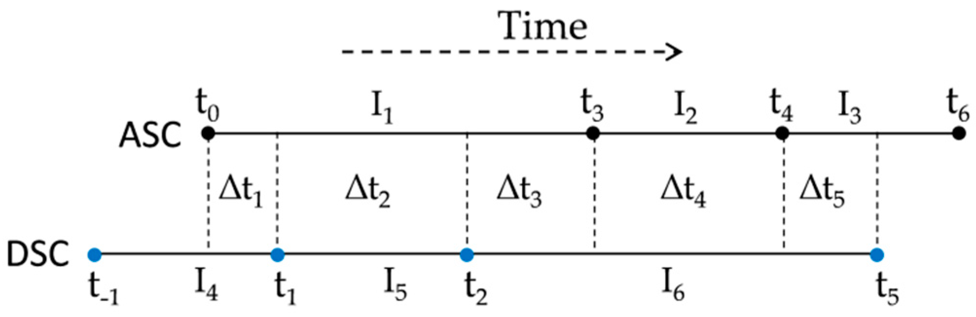
where is the radar azimuth angle, 14.2 (ascending) and 165.2 (descending) in our case, and is the average incidence angle, 33.5 (ascending) and 33.7 (descending) in our case. ∆t is the time interval between the two images of the interferogram and is a regularization parameter, is an identity matrix. The regularization parameter is used to regularize the solution. The larger the value, the smoother the solution. The L-curve method can be used to select the optimal value [42]. and are the average deformation rates in the vertical and east-west direction, D is the observed (unwrapped) interferometric displacement. As shown in Figure 2, the first image from the descending path is acquired earlier than that of the ascending image, and we compensate the first descending interferogram by a factor of ; similarly the last ascending interferogram is compensated by a factor of . After applying boundary correction, the first and last image acquisition dates are assumed to be at and for the ascending and descending images [29]. Then, we can obtain more detailed ground surface deformation caused by fluid extraction or injection by MSBAS method.
3.3. Data and Processing
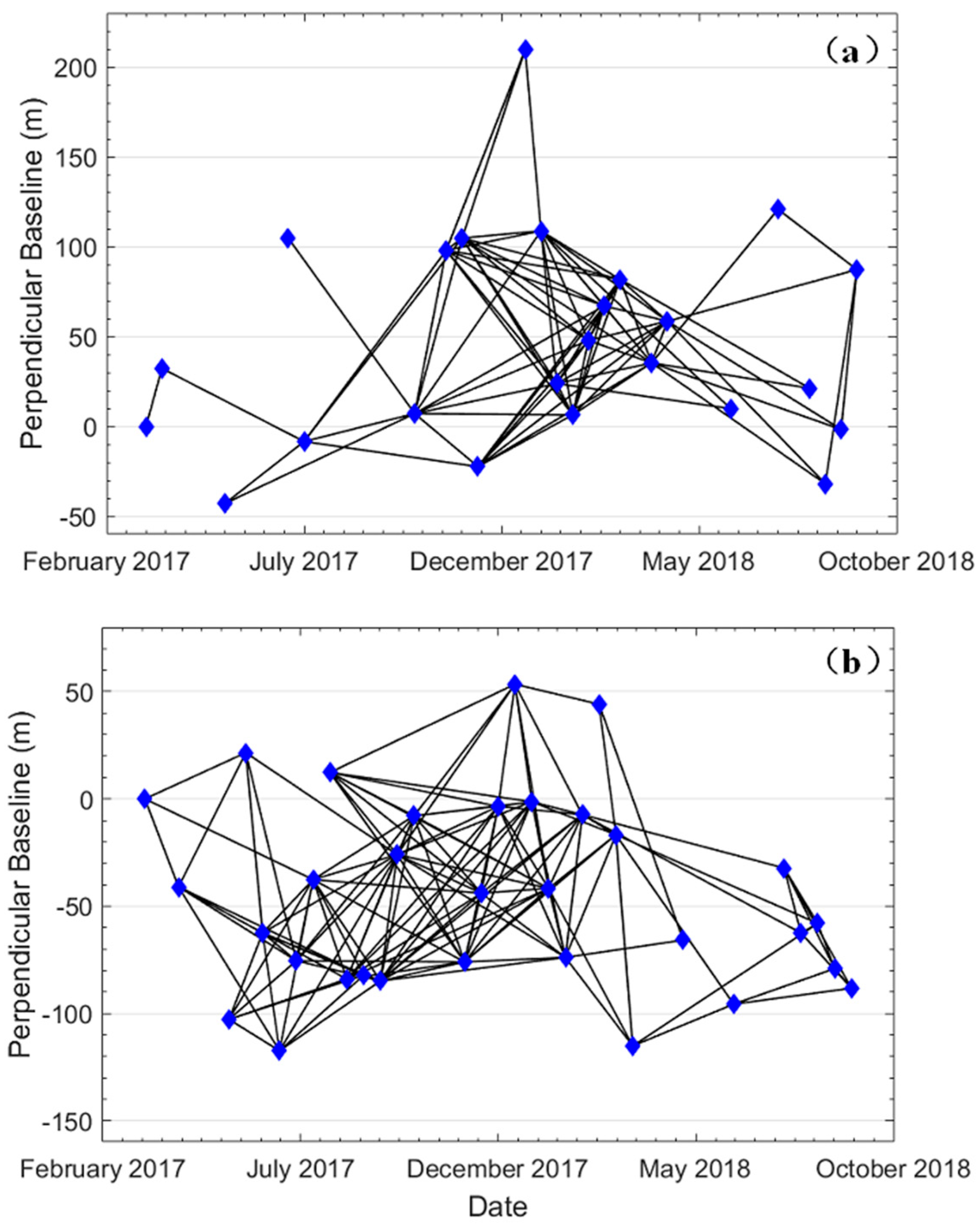
SAR images covering the study area were acquired by C-band (5.6 cm wavelength and 5.4 GHz) radar on board the European Space Agency (ESA) Sentinel-1 A/B satellites. Sentinel A and Sentinel B are the latest generation of C-band satellites launched by ESA in 2014 and 2016, respectively; the coherence between images is increased compared with previous ESA satellites, because of a reduced revisit time (12 days for Sentinel A, and 6 days for the combination of Sentinel A and B) [43]. The image in wide swath mode provides a wide coverage of about 250 km with a slant range resolution of 5 m and an azimuth resolution of 20 m. In this study, we used GAMMA software to process 32 ascending (Figure 3a) and 34 descending (Figure 3b) datasets, gathered between March 2017 and August 2018 [44]. There are two kinds of orbital data files provided by ESA, including correctional orbital parameters with accuracy within 10 cm and precise orbital ephemeris parameters with accuracy within 5 cm [45]. The latter were used to improve the accuracy of the satellite position and decrease the perpendicular baseline error. We chose spatial perpendicular baselines smaller than 100 m and temporal baselines smaller than 100 days as the thresholds of the interferograms. Interferograms with good coherence and small atmospheric errors were selected for further processing. As a result, we obtained 82 ascending (Figure 3a) and 131 descending (Figure 3b) interferograms. A digital elevation model (DEM) with 1 arc-second (about 30 m resolution) from the Shuttle Radar Topography Mission (SRTM) (http://srtm.csi.cgiar.org) was used to remove topographic effects from the interferograms. Adaptive filtering was used to filter the interferograms [46], and the minimum cost flow (MCF) algorithm was used to unwrap them [47].
4. Results
4.1. Deformation Velocity
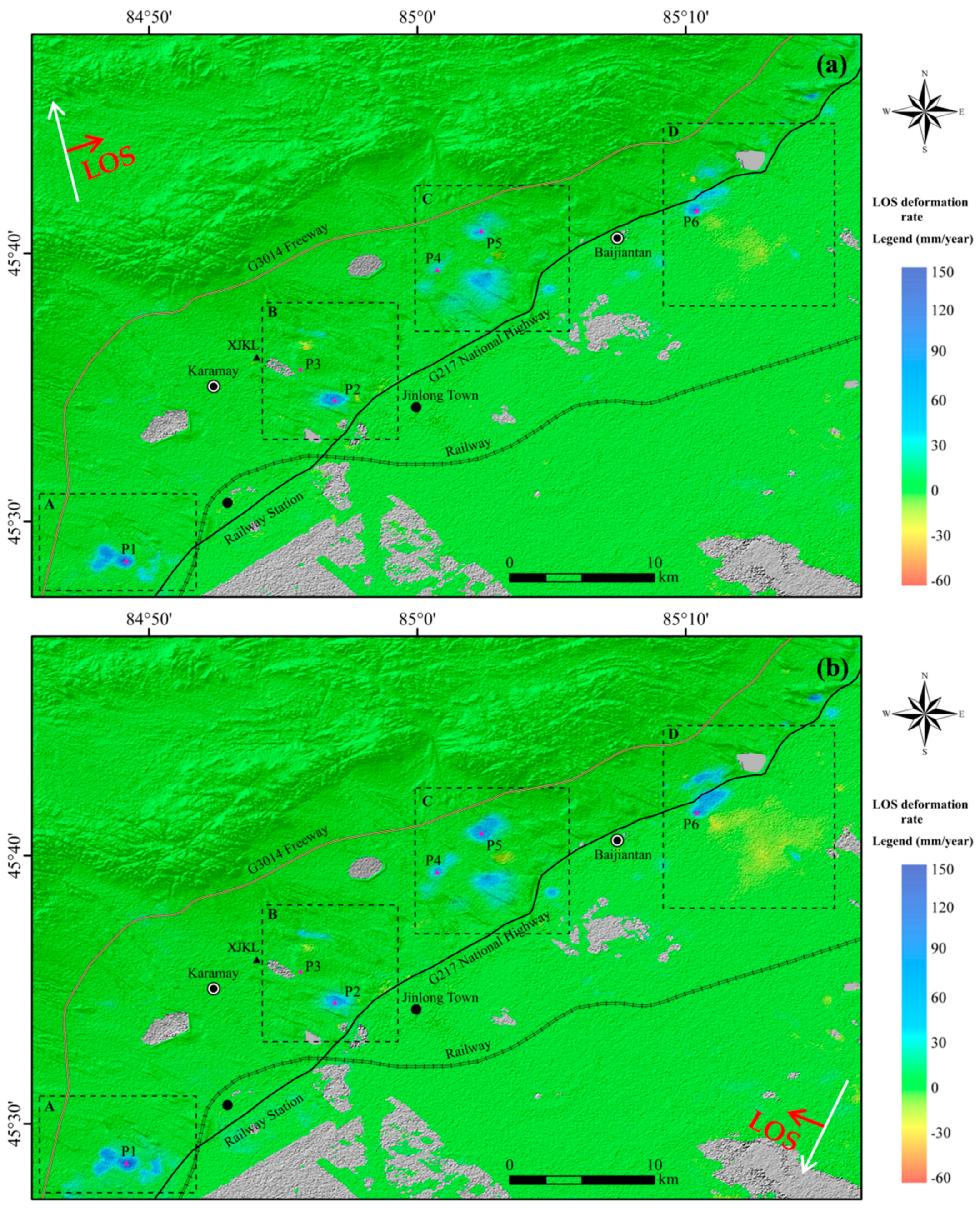
The annual average deformation rate (Figure 4) in the line of sight (LOS) over the Karamay oilfield area was obtained using the stacking method (Equation (1)). The deformation rates from ascending and descending orbits exhibited a good consistency in magnitude. There were four obvious uplift areas (marked as A, B, C and D in Figure 4) and one subsidence center. The maximum rate of subsidence was about 32 mm/year. The maximum rate of uplift, exceeding 100 mm/year, appeared in area A.
Compared with previous research results [6,25], the uplift deformation rate changed from 30 mm/year between 2003 and 2010 to 150 mm/year from 2017 to 2018. The region with the largest deformation rate occurred in Zone B from 2003 to 2010, while the region with the largest deformation rate occurred in Zone A from 2017 to 2018. We suspect that these phenomenon may be caused by the transfer of main oil exploration area from Zone B to Zone A, which needs to be confirmed by the oilfield mining company.
4.2. Two-Dimensional Time Series Deformation
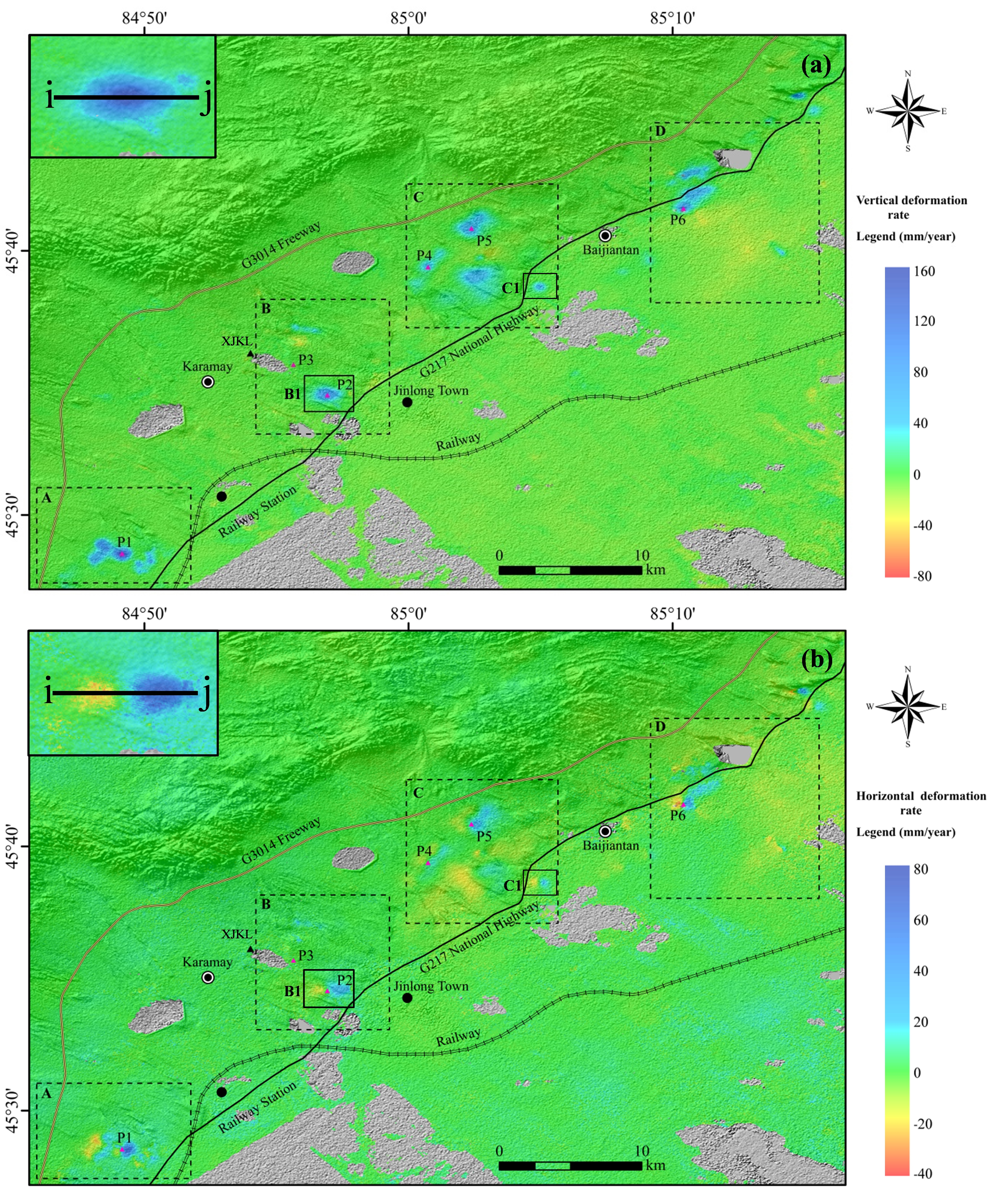
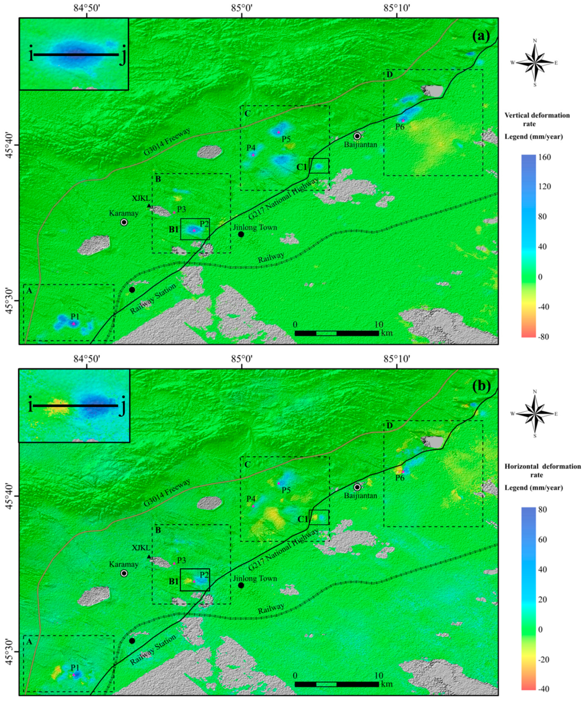
In order to derive the vertical and horizontal components of deformation of the ground surface, we applied the MSBAS method (Equation (2)) to obtain the two-dimensional time series deformation field (east–west and vertical) of the study area [40,48]. The vertical and the east–west deformation rates are presented in Figure 5a,b, respectively. Both vertical and east–west displacements occurred in the four deformation zones and are marked in Figure 5 (A, B, C and D).
The maximum uplift rate was up to 160 mm/year, and the maximum eastward movement rate was 65 mm/year in area A (Figure 5). Area B was also a typical uplift area with horizontal motion. The magnitude of the uplift was about 110 mm/year, and the east flank of the uplifted center moved eastward at a rate of 30 mm/year, and the west side of the uplifted center moved westward at a rate of 15 mm/year. The uplift rate at area C was approximately 80 mm/year and there was also a small area with subsidence rate of 16 mm/year. Area D exhibited both uplift and obvious subsidence; uplift was at a rate of approximately 110 mm/year and the subsidence rate was approximately 25 mm/year. Although there were varying degrees of east–west and vertical deformation in the four study areas, the vertical displacement was dominant.
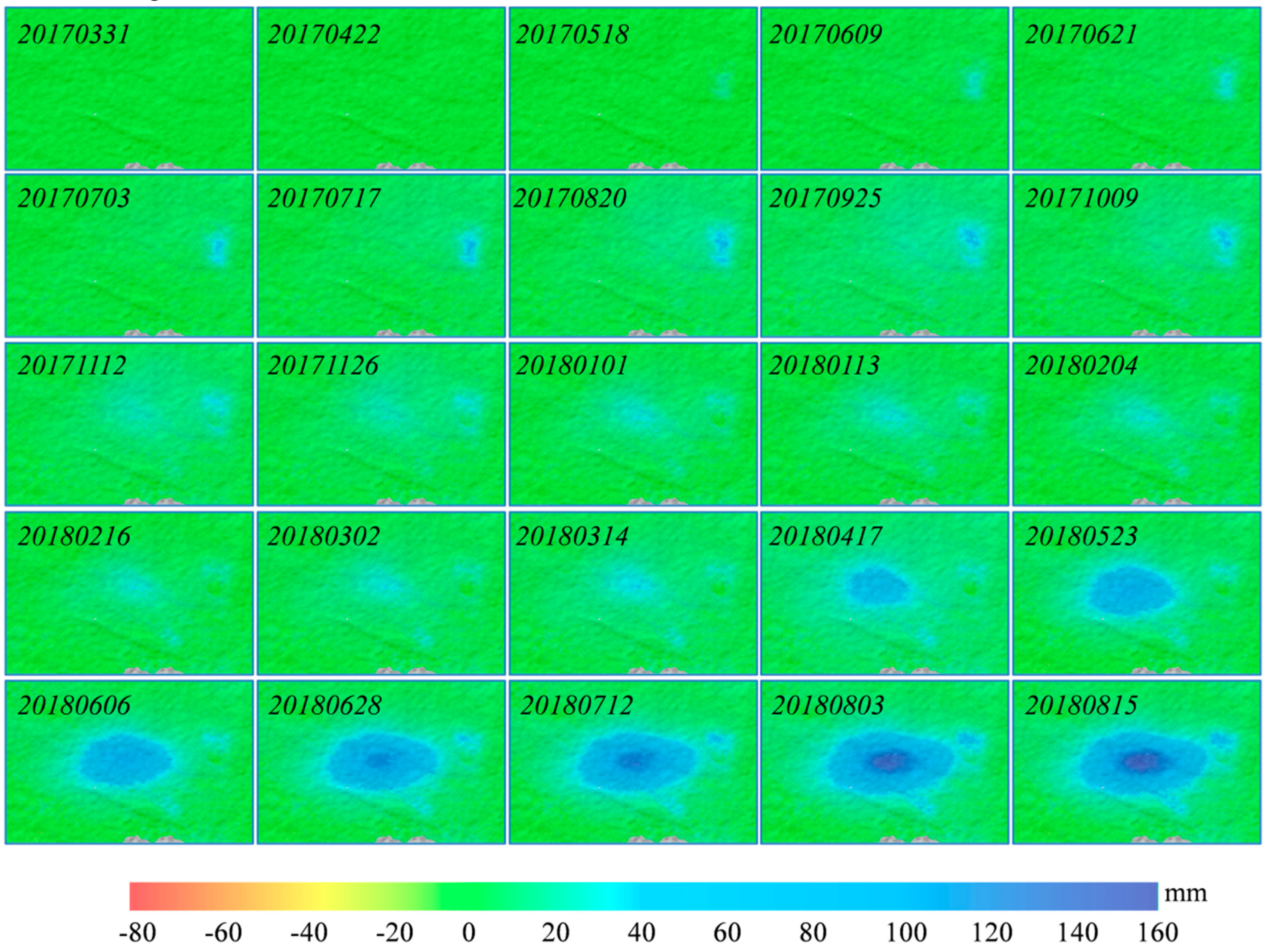
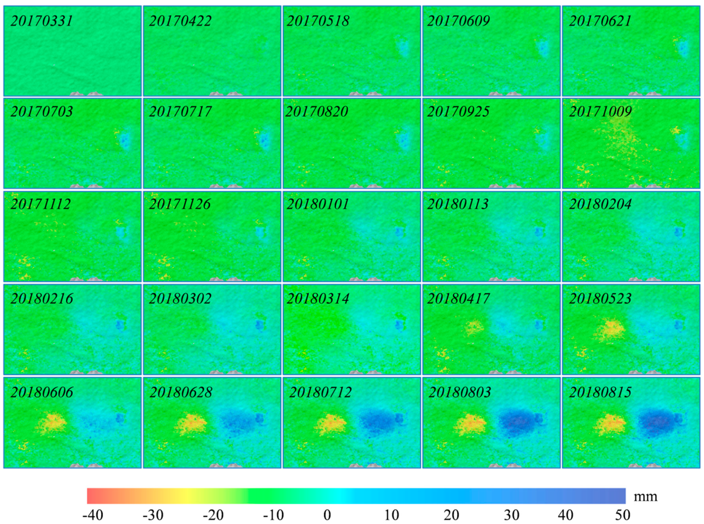
In order to study the deformation process of the uplift zone, area B1 (Figure 5) was selected for examination of its two-dimensional time series deformation in the vertical (Figure 6) and east–west directions (Figure 7).
The vertical deformation rate of the area increased slowly with time before March 2018, but significantly accelerated thereafter (Figure 6). The magnitude of the uplift reached approximately 160 mm by 15 August 2018. Similarly, the east–west deformation rate was also slow before March 2018 and the horizontal motion intensified after March 2018 (Figure 7). The amounts of westward displacement on the western flank of the uplift reached 30 mm, and eastward movement on the other side was closed to 60 mm. Several previous studies have shown that fluid injection, a commonly used method in oil and gas production, can lead to ground uplift [6,26]. This may be related to enhanced water injection and production activities. The increase of pore pressure with fluid injection leads to a decrease of the effective stress of the reservoir, which leads to uplift of the ground surface [27]. Therefore, we speculated that the deformation in this area was likely to be related to liquid injection activities during oil and gas production. Rapid ground deformation may pose a threat to underground pipeline facilities and surface constructions [49]. Therefore, oil and gas production managers should pay attention to it.
5. Analysis and Discussion
5.1. Deformation Analysis
GPS measurements at station XJKL (triangle in Figure 5) were obtained from (ftp://ftp.cgps.ac.cn/products/position/gamit/XJKL.ios_gamit_detrend.neu) (Global Navigation Satellite System Data Products of China Earthquake Administration). They were used to evaluate the reliability of the InSAR results (Figure 8). This comparison shows that the InSAR and GPS observations are in good agreement. Keeping in mind that the GPS station XJKL is a station from China Mainland Tectonic Environment Monitoring Network Project. The horizontal displacement of XJKL refers to the International GNSS Service (IGS) station information of neighboring countries or regions [50]. Therefore, the horizontal displacement on the XJKL station represents the tectonic movement over a large area. However, the horizontal displacement from InSAR is very local. This may result in the horizontal displacements from InSAR being less than that in XJKL.
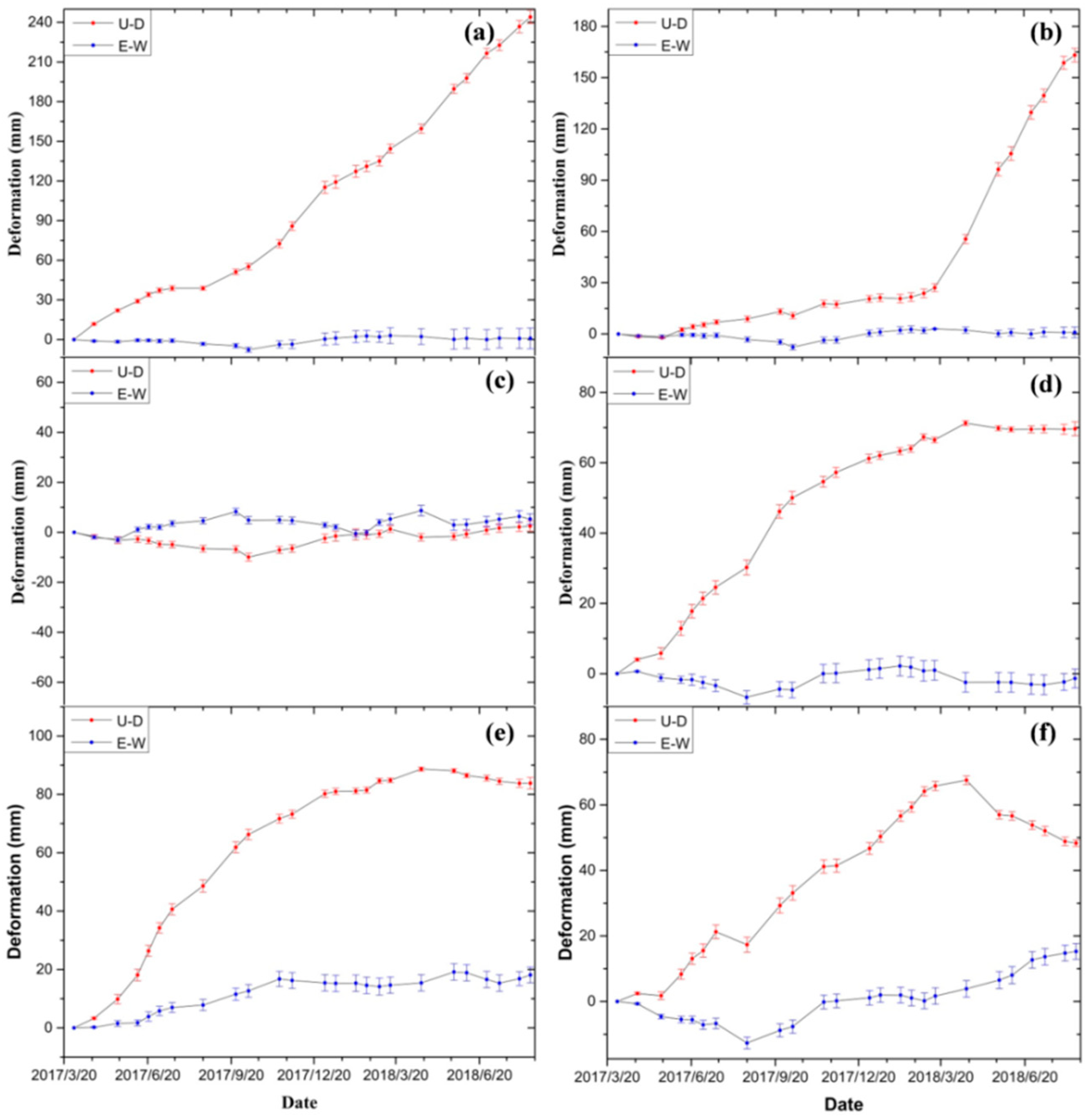
In order to study the time-varying characteristics of surface deformation, time series InSAR results at six points were extracted (Figure 5). In order to avoid the influence of inconsistent precision at individual pixels, the average value of 5 × 5 pixels, i.e., 150 m × 150 m around each point was used to plot the time series results (Figure 9).
Point P3 (in Figure 5) located at Jinlong Town is away from the obvious deformation zone, and the other selected points are near the center of uplifting of each deformation zone. The horizontal and vertical displacements at point P3 (Figure 9c) oscillated slightly around 0 with time, indicating that the results we obtained were reliable. The uplift center P1 (Figure 9a), located 6 km southwest of the railway station, showed close to a linear rate of uplift with time. By August 2018, the relative uplift was about 240 mm. The maximum deformation rate reached 160 mm/year from 2017 to 2018. This result is different from a previously reported maximum deformation rate of 50 mm/year from 2006 to 2010 [6,26]. According to the report, the oil reservoirs in the Karamay oilfield area generally entered a high moisture cut period after 2015. In order to ensure oil production, increasing water injection was taken after 2015 [51]. Therefore, continuous fluid injection activity may be a factor that caused continued uplift. Unlike P1, P2 in area B (Figure 5), located to the west of Jinlong Town, exhibited a slow uplift before March 2018, reaching approximately 30 mm (Figure 9b). However, the magnitude of the uplift increased to 130 mm from March 2018 to August 2018, which may have been related to enhanced injection and production activities in this area.
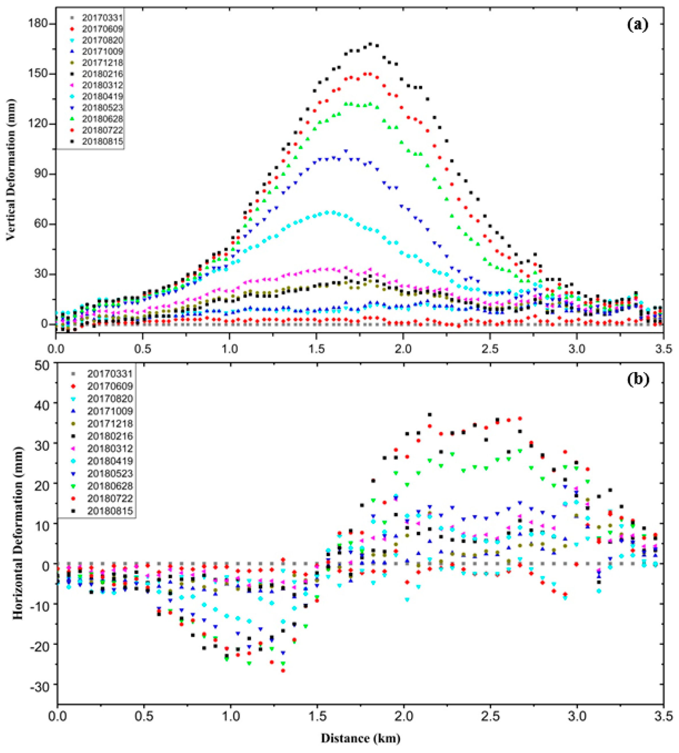
We selected images from Figure 5a,b at regular time intervals to make time series profiles of uplift deformation and east–west displacement. Deformation time series along profile i–j in Figure 5 highlight the spatiotemporal progress of uplift and east–west movement (Figure 10) in the vertical (a) and east–west (b) directions. Similar deformation modes were apparent points P4 and P5 on the west side of the Baijiantan (Figure 9d,e). The displacement of P4 and P5 increased with time, and the deformation was relatively small after March 2018. Uplift in the early stage and a tendency to subsidence in the later stage was apparent at point P6, located to the east of Baijiantan (Figure 9f). This phenomenon may be due to the injection of liquid in the early stage, leading to the uplift. The oil exploitation caused the later subsidence. Deformation in area D occurred near the national highway G217 (Figure 5) and has potential to threaten road stability and the nearby oil/gas pipelines.
5.2. Inversion Modeling
Geophysical inversion in our study is based on monitoring data and applying a corresponding physical model to explore model parameters and reservoir characteristics. Because the ground uplift was induced by reservoir expansion, it provides valuable information allowing us to evaluate the dynamic changes in reservoir properties [52]. Using the deformation information acquired by InSAR and the corresponding geophysical model, reservoir parameter values can be inverted to better understand the underground fluid injection and surface dynamics [3]. Compared to other existing models, only physical models from Mogi [53] and Sill [54] are commonly used to explain ground surface deformation caused by changes in underground filling. Therefore, both models were selected to perform parameter inversion for uplift areas B1 and C1 (see Figure 5), in order to explain surface uplift behavior in this study.
5.2.1. Mogi Modeling
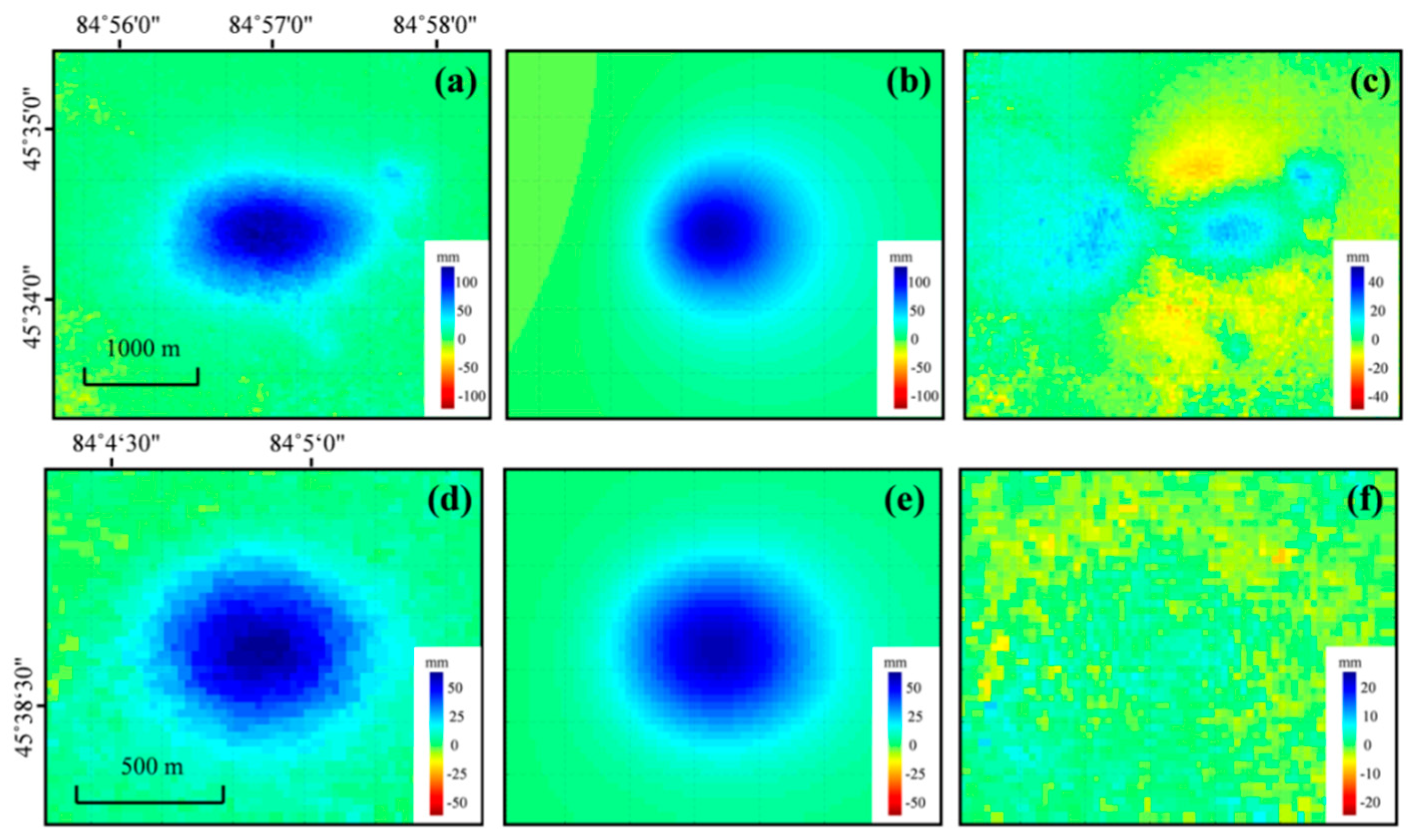
The Mogi model is a simple and effective inversion model of surface deformation arising from pressure changes of underground reservoirs [53]. The simulated parameters include point source center position (X, Y), reservoir depth and volume change. The vertical cumulative deformation maps (Figure 7) were used to invert the reservoir parameters. The root mean square error (RMSE) between the observed and modeled values was used as inversion criterion. Table 1 shows the best fitting parameters obtained by the Mogi model. Volume changes in areas B1 and C1 are 1.97 × 10⁵ m3 and 3.87 × 10⁴ m3, respectively. Most of the residuals were smaller than 10 mm (Figure 11c,f). However, a relatively large residual occurred on the long axis of the elliptical deformation for B1. This observation indicates that the point source Mogi model is suitable for circular surface deformation, but when the deformation of the surface approximates an ellipse, it does not perform well anymore. For area C1, the deformation characteristics are close to circular, so the Mogi model performs adequately.
5.2.2. Sill Modeling
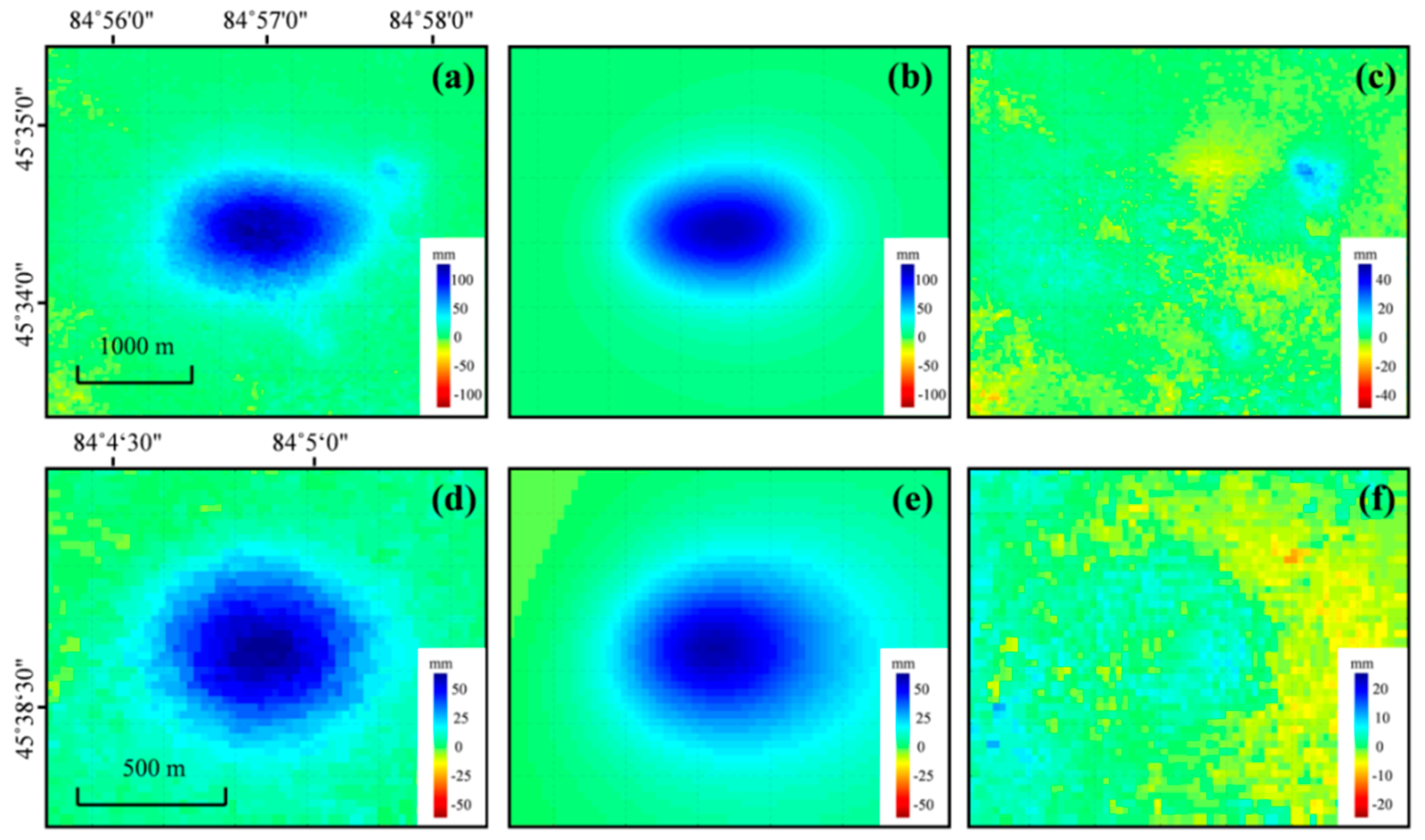
We also modeled oilfield deformation to explain the subsurface processes and explain the integral uplift pattern of the ground with the Sill model [54]. The Sill model, embedded in an elastic half-space, is defined by seven parameters: Location (X, Y), depth, strike, length, width, and opening. The RMSE between the observed and modeled values was used as inversion criterion. The optimal parameters of the Sill simulation are shown in Table 2. The calculated reservoir depth in areas B1 and C1 were 606 m and 422 m, respectively. One source with a rectangular sill of size 996 × 230 m, below the deformation area B1, was directed toward 270° from the north (anticlockwise). Another source with a rectangular sill 289 × 256 m, below area C1, was directed 189° from the north (anticlockwise). The residuals (Figure 12c,f) were mostly concentrated between 15 mm and 15 mm. Although we used a uniform elastic half-space model [54], the geology of the study area has some heterogeneities, which may affect the inversion results to some extent.
Comparing the results from the two models (Table 1 and Table 2), the depths were close and were consistent with the depth of the oil well in this area [55]. In area B1, the maximum volume changes from the Mogi model and the minimum volume change from the Sill model (2.08 × 10⁵ and 2.15 × 10⁵ m3, respectively) were very similar to each other. Similar to the C1 area, the volume changes (3.2 × 10⁴ to 4.4 × 10⁴ m3) from Mogi model were also close to the volume changes (2.2 × 10⁴ to 3.5 × 10⁴ m3) from Sill model. Unfortunately, we cannot compare our modeled volumes with the actual volume mined, because it is not available in the published data.
5.3. Deformation and Seismicity
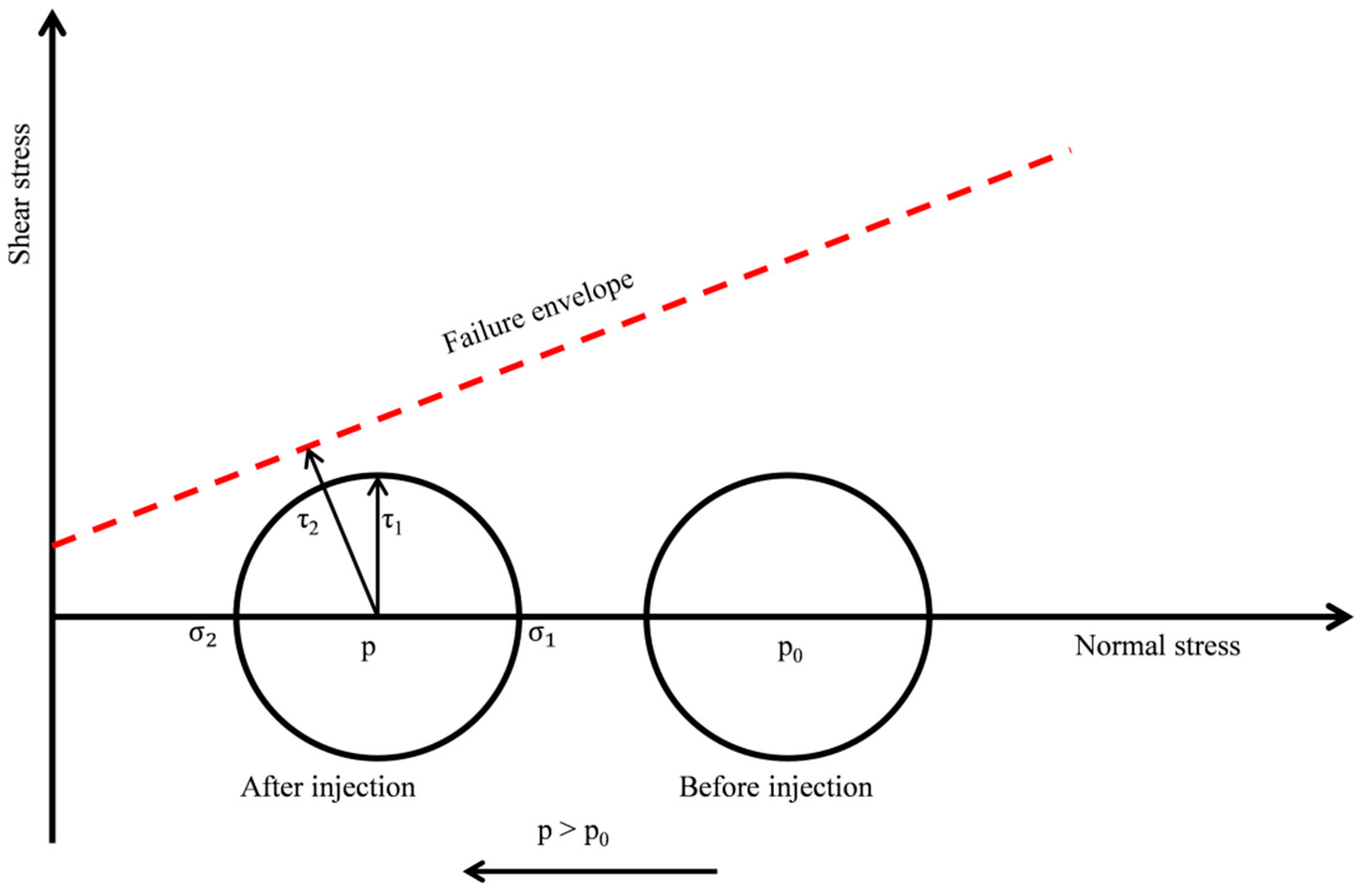
Prior to liquid injection, the stress state is determined by local tectonic stress, which may cause new geomechanical processes after liquid injection [27]. Increased pore pressure due to fluid injection reduces the effective stress, which causes the reservoir to expand and act on the surface to cause ground uplift. This mechanism is easier to understand with the Mohr–Coulomb circles (Figure 13), which is modified from Teatini [26]. According to Terzaghi’s principle, when a fluid is injected into the tiny pores of the rock, the pore pressure will increase, resulting in a decrease in the effective stress of the rock. The Mohr circle shifts to the left as effective stress decreases. There are maybe two outcomes when the Mohr circle continues to move left: (1) A shear failure may happen if the circle is tangent to the envelope; and (2) a tensile damage may occur when the circle intersects the envelope [27]. The new stress is closer to the failure envelope than before the injection because of the injection of fluid, which may induce seismicity [56].
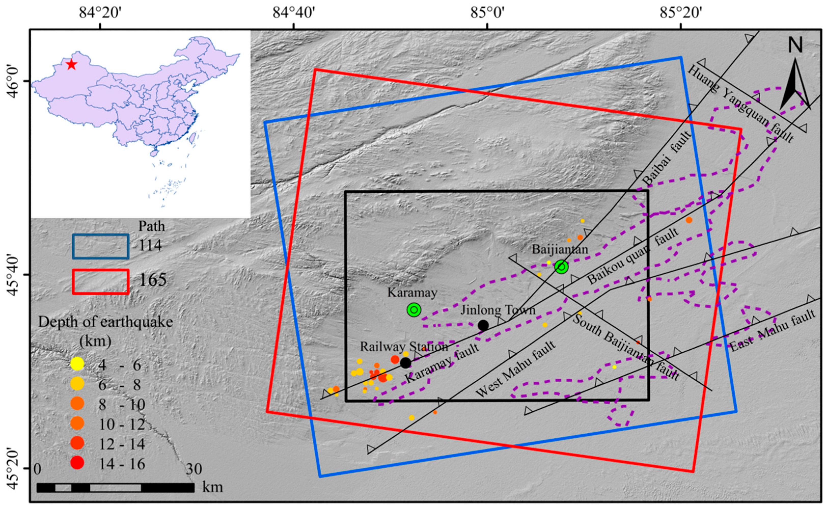
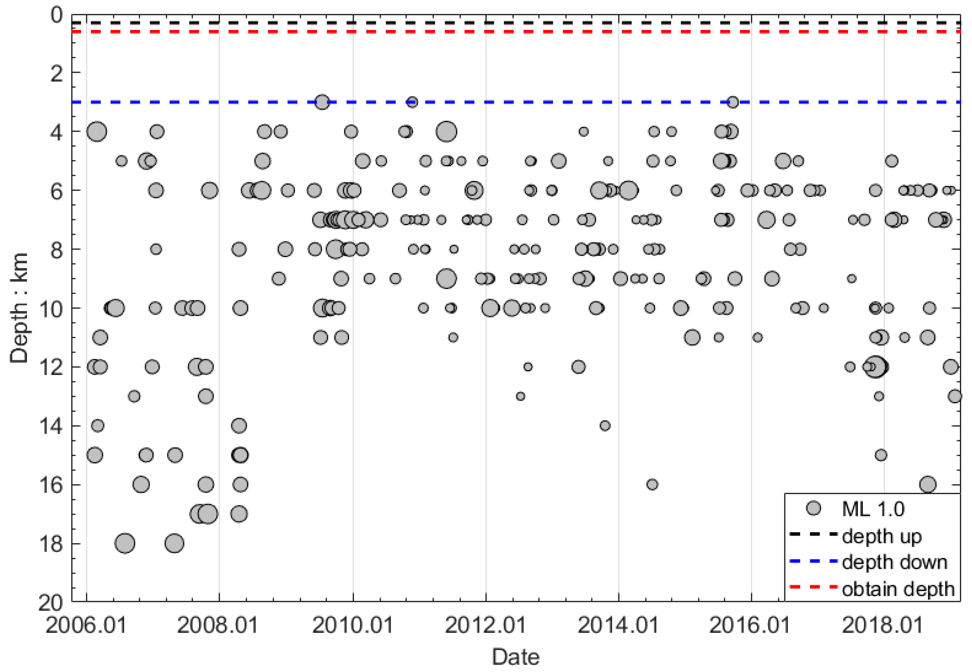
We used seismic data of magnitude 1.0 or higher within 70 km of the oilfield from March 2017 to August 2018 from the China Earthquake Data Center (http://data.earthquake.cn). These data are plotted in Figure 1 and Figure 14. The locations of seismicity are mainly distributed near faults, especially near the Karamay fault (Figure 1). The earthquake epicenters mainly occur near the Baibai fault, West Mahu fault, and the Baiquankou fault. In Figure 14, the depth of the inversion reservoir is about 600 m (red line), and as mentioned earlier, the depth of the reservoir is from 300 (black line) to 3000 meters (blue line). However, the depth of the earthquakes are greater than 3000 m. So based on the location and depth of earthquakes in study area, we suggest that the occurrence of the earthquakes in this region is not related to the activities associated with oil production.
6. Conclusions
In this study, we monitored deformation induced by processes associated with oil production at the Karamay oilfield by analyzing Sentinel images acquired from March 2017 to August 2018. We have reached the following main conclusions:
1. The surface deformation caused by oil mining was still significant between 2017 and 2018. Four uplift zones and one settling zone were found in the oilfield. The maximum lifting deformation rate exceeded 160 mm/year, and the maximum subsidence was approximately 32 mm/year. Time series deformation results show that enhanced injection and production activities may cause nonlinear surface deformation.
2. Two-dimensional (vertical and east–west) time series deformation maps were derived by the MSBAS. The results show that the east–west deformation induced by oil mining cannot be ignored in the Karamay oilfield.
3. There was no direct relationship between the occurrence of earthquakes near the oilfield and the activities associated with oil production in Karamay oilfield from 2017 to 2018.
4. If combined with liquid injection data and oil extraction data, time series InSAR results could play a significant role in evaluating future uplift hazards and alerting oil companies of the possible risks.
Unfortunately, the liquid injection data and oil extraction data are not available at this time because of their proprietary. It should be noted that these data should be collected for future research.
Author Contributions
Conceptualization, C.Y., D.Z. and C.Z.; methodology, D.Z. and C.Y.; software, D.Z. and B.H.; validation, C.Y. and C.Z.; investigation, L.C. and D.Z.; data analysis, D.Z., R.S. and J.D.; writing—original draft preparation, D.Z.; writing—review and editing, all the authors; funding acquisition, C.Y. and C.Z.
Funding
This research was funded jointly by the National Natural Science Foundation of China (NSFC) (Nos. 41731066, 41628401, 41790445, 41604015, and 41604001), the China Geological Disaster Investigation Project (DD20190637), the State’s Key Project of Research and Development Plan (2018YFC1504805), the Fundamental Research Funds for the Central Universities (CHD,300102269204), and the Shanxi Provincial Natural Science Basic Research Project (2019JM-245).
Acknowledgments
We acknowledge the European Space Agency (ESA) for freely making available the Sentinel-1A/B data. Thanks to the excellent software MSBAS, which can be freely downloaded from the following website, https://insar.ca/software/msbasv3.
Conflicts of Interest
The authors declare no conflict of interest.
References
- Li, X.; Li, W.; Gao, B.; Yang, D. Study on subsurface water injection in Qizhong area of Karamay oilfield. Xinjiang Oil Gas. 2012, 3, 57–59. [Google Scholar]
- Pan, S. Discussion on oil exploitation technology and oil field water Injection. Chem. Intermed. 2018, 7, 70–71. [Google Scholar]
- Khakim, M.Y.N.; Tsuji, T.; Matsuoka, T. Geomechanical modeling for InSAR-derived surface deformation at steam-injection oil sand fields. J. Pet. Sci. Eng. 2012, 96, 152–161. [Google Scholar] [CrossRef]
- Guéguen, Y.; Deffontaines, B.; Fruneau, B.; Al Heib, M.; de Michele, M.; Raucoules, D.; Planchenault, J.; Guise, Y. Monitoring residual mining subsidence of Nord/Pas-de-Calais coal basin from differential and Persistent Scatterer Interferometry (Northern France). J. Appl. Geophys. 2009, 69, 24–34. [Google Scholar] [CrossRef]
- Martínez-Garzón, P.; Kwiatek, G.; Bohnhoff, M.; Dresen, G. Volumetric components in the earthquake source related to fluid injection and stress state. Geophys. Res. Lett. 2017, 44, 800–809. [Google Scholar] [CrossRef] [Green Version]
- Ji, L.; Zhang, Y.; Wang, Q.; Xin, Y.; Li, J. Detecting land uplift associated with enhanced oil recovery using InSAR in the Karamay oil field, Xinjiang, China. Int. J. Remote Sens. 2016, 37, 1527–1540. [Google Scholar] [CrossRef]
- Lu, Z.; Dzurisin, D. InSAR imaging of Aleutian volcanoes. In InSAR Imaging of Aleutian Volcanoes; Springer: Berlin/Heidelberg, Germany, 2014; pp. 87–345. [Google Scholar]
- Massonnet, D.; Briole, P.; Arnaud, A. Deflation of Mount Etna monitored by spaceborne radar interferometry. Nature 1995, 6532, 567–570. [Google Scholar] [CrossRef]
- Lu, Z.; Mann, D.; Freymueller, J.T.; Meyer, D.J. Synthetic aperture radar interferometry of Okmok volcano, Alaska: Radar observations. J. Geophys. Res. Solid Earth 2000, B5, 10791–10806. [Google Scholar] [CrossRef]
- Massonnet, D.; Rossi, M.; Carmona, C.; Adragna, F.; Peltzer, G.; Feigl, K.; Rabaute, T. The displacement field of the landers earthquake mapped by radar interferometry. Nature 1933, 64, 138–142. [Google Scholar] [CrossRef]
- Zebker, H.A.; Rosen, P.A.; Goldstein, R.M.; Gabriel, A.; Werner, C.L. On the derivation of coseismic displacement fields using differential radar interferometry: The landers earthquake. J. Geophys. Res. Solid Earth 1994, 99, 19617–19634. [Google Scholar] [CrossRef]
- Tantianuparp, P.; Shi, X.; Zhang, L.; Balz, T.; Liao, M. Characterization of landslide deformations in three Gorges area using Multiple InSAR Data Stacks. Remote Sens. 2013, 5, 2704–2719. [Google Scholar] [CrossRef]
- Zhao, C.; Lu, Z.; Zhang, Q.; Fuente, J.D.L. Large-area landslide detection and monitoring with ALOS/PALSAR imagery data over Northern California and Southern Oregon, USA. Remote Sens. Environ. 2012, 124, 348–359. [Google Scholar] [CrossRef]
- Goldstein, R.M.; Engelhardt, H.; Kamb, B.; Frolich, R.M. Satellite radar interferometry for monitoring ice sheet motion: Application to an Antarctic ice stream. Science 1993, 262, 1525–1530. [Google Scholar] [CrossRef] [PubMed]
- Michel, R.; Rignot, E. Flow of Glaciar Moreno, Argentina, from repeat-pass Shuttle Imaging Radar images: Comparison of the phase correlation method with radar interferometry. J. Glaciol. 1999, 45, 93–100. [Google Scholar] [CrossRef]
- Lubis, A.M.; Sato, T.; Tomiyama, N.; Isezaki, N.; Yamanokuchi, T. Ground subsidence in Semarang-Indonesia investigated by ALOS–PALSAR satellite SAR interferometry. J. Asian Earth Sci. 2011, 40, 1079–1088. [Google Scholar] [CrossRef]
- Zhao, C.; Zhang, Q.; Ding, X.; Peng, J. Research on the characteristics of land subsidence and ground fissure development in Xi’an based on InSAR. J. Eng. Geol. 2009, 5, 1214–1222. [Google Scholar]
- Milillo, P.; Giardina, G.; DeJong, M.J.; Perissin, D.; Milillo, G. Multi-Temporal InSAR structural damage assessment: The London crossrail case study. Remote Sens. 2018, 10, 287. [Google Scholar] [CrossRef]
- Giardina, G.; Milillo, P.; DeJong, M.; Perissin, D.; Milillo, G. Evaluation of InSAR monitoring data for post-tunnelling settlement damage assessment. Struct. Control Health Monit. 2019, 26, e2285. [Google Scholar] [CrossRef]
- Roccheggiani, M.; Piacentini, D.; Tirincanti, E.; Perissin, D.; Menichetti, M. Detection and monitoring of tunneling induced ground movements using Sentinel-1 SAR interferometry. Remote Sens. 2019, 11, 639. [Google Scholar] [CrossRef]
- Juncu, D.; Árnadóttir, T.; Geirsson, H.; Guðmundsson, G.B.; Lund, B.; Gunnarsson, G.; Michalczewska, K. Injection-induced surface deformation and seismicity at the Hellisheidi geothermal field, Iceland. J. Volcanol. Geotherm. Res. 2018. [Google Scholar] [CrossRef]
- Yang, Q.; Zhao, W.; Dixon, T.H.; Amelung, F.; Han, W.S.; Li, P. InSAR monitoring of ground deformation due to CO2 injection at an enhanced oil recovery site, West Texas. Int. J. Greenh. Gas Control 2015, 41, 20–28. [Google Scholar] [CrossRef] [Green Version]
- Loesch, E.; Sagan, V. SBAS analysis of induced ground surface deformation from wastewater injection in east central Oklahoma, USA. Remote Sens. 2018, 10, 283–299. [Google Scholar] [CrossRef]
- Zhu, Z.; Du, M.; Han, H. New technology for shallow super heavy oil exploitation in Karamay oilfield. J. Oil Gas Technol. 2007, 3, 441–443. [Google Scholar]
- Pang, P. Karamay oilfield—the first large oilfield in New China. J. Univ. Pet. China 2001, 4, 29–32. [Google Scholar]
- Aimaiti, Y.; Yamazaki, F.; Liu, W.; Kasimu, A. Monitoring of land-surface deformation in the Karamay oilfield, Xinjiang, China, Using SAR Interferometry. Appl. Sci. 2017, 7, 772–787. [Google Scholar] [CrossRef]
- Teatini, P.; Gambolati, G.; Ferronato, M.; Settari, A.; Walters, D. Land uplift due to subsurface fluid injection. J. Geodyn. 2011, 51, 1–16. [Google Scholar] [CrossRef] [Green Version]
- Samsonov, S.; d’Oreye, N. Multidimensional time-series analysis of ground deformation from multiple InSAR data sets applied to Virunga volcanic province. Geophys. J. Int. 2012, 191, 1095–1108. [Google Scholar]
- Samsonov, S.V.; Feng, W.; Peltier, A. Multidimensional Small Baseline Subset (MSBAS) for volcano monitoring in two dimensions: Opportunities and challenges. Case study Piton de la Fournaise volcano. J. Volcanol. Geotherm. Res. 2017, 344, 121–138. [Google Scholar] [CrossRef]
- Samsonov, S.V.; D’oreye, N. Multidimensional Small Baseline Subset (MSBAS) for two-dimensional deformation analysis: Case study Mexico City. Can. J. Remote Sens. 2017, 18, 318–329. [Google Scholar] [CrossRef]
- Song, Z.Q.; Tan, C.Q.; Liu, S.S.; Wu, S.B.; Gao, X.J.; Qin, J.H.; Luo, Z.X. Study on reserve distribution and recovery percent of Heterogenerous conglomerate oil pools—an example front Upper Karamay formation reservoir in Karamay oilfield. Xinjiang Pet. Geol. 2001, 22, 335–337. [Google Scholar]
- Zi-qi, S.; Hong, W.; Jun-feng, Y.; Wei, H.; Ting, P.; Kun-Peng, C. The research of reservoir tectonic feature of Karamay group in Qizhong and Qidong area in Karamay oilfield. West China Pet. Geosci. 2006, 4, 46–49. [Google Scholar]
- Wang, Y. Glutenite Reservoir Heterogeneity Study of Upper Karamay Formation in Wu2dong Area of Karamay Oilfield; China University of Petroleum: Beijing, China, 2016. [Google Scholar]
- Yin, S.; Chen, G.; Chen, Y.; Wu, X. Control effect of pore structure modality on remaining oil in glutenite reservoir: A case from lower Karamay Formation in block Qidong 1 of Karamay oilfield. Lithhologic Reserv. 2018, 30, 91–102. [Google Scholar]
- Sandwell, D.T.; Price, E.J. Phase gradient approach to stacking interferograms. J. Geophys. Res. Solid Earth 1998, 103, 30183–30204. [Google Scholar] [CrossRef] [Green Version]
- Sandwell, D.T.; Sichoix, L. Topographic phase recovery from stacked ERS interferometry and a low-resolution digital elevation model. J. Geophys. Res. Solid Earth 2000, 105, 28211–28222. [Google Scholar] [CrossRef]
- Ali, S.T.; Feigl, K.L. A new strategy for estimating geophysical parameters from InSAR data: Application to the Krafla central volcano in Iceland. Geochem. Geophys. Geosystems 2012, 13. [Google Scholar] [CrossRef] [Green Version]
- Liu, C. Research on Time Series InSAR Technology for Structural Deformation Monitoring; Chang’an University: Xi’an, China, 2017. [Google Scholar]
- Wright, T.J. Toward mapping surface deformation in three dimensions using InSAR. Geophys. Res. Lett. 2004, 31, 169–178. [Google Scholar] [CrossRef]
- Jin-Woo, K.; Zhong, L.; Kimberly, D. Ongoing deformation of sinkholes in Wink, Texas, observed by time-series Sentinel-1A SAR interferometry. Remote Sens. 2016, 4, 313–324. [Google Scholar]
- Samsonov, S.; Czarnogorska, M.; White, D. Satellite interferometry for high-precision detection of ground deformation at a carbon dioxide storage site. Int. J. Greenh. Gas Control 2015, 42, 188–199. [Google Scholar] [CrossRef]
- Hansen, P.C.; O’Leary, D.P. The use of the L-Curve in the regularization of discrete ill-posed problems. SIAM J. Sci. Comput. 1993, 6, 1487–1505. [Google Scholar] [CrossRef]
- Ouyang, L.; Li, X.; Hui, F.; Zhang, B.; Cheng, X. Sentinel-1A data products’ characters and the potential applications. Chin. J. Polar Res. 2017, 29, 286–295. [Google Scholar]
- Werner, C.; Wegmüller, U.; Strozzi, T.; Wiesmann, A. Gamma SAR and interferometric processing software. In Proceedings of the Ers-Envisat Symposium, Gothenburg, Sweden, 16–20 October 2000; pp. 1620–1629. [Google Scholar]
- Zhang, Y.; Wang, P.; Luo, X.; Zhang, Q.; Chen, H. Monitoring Xi’an land subsidence using Sentinel-1 images and SBAS-InSAR technology. Bull. Surv. Mapp. 2017, 29, 100–104. [Google Scholar]
- Goldstein, R.M.; Werner, C.L. Radar interferogram filtering for geophysical applications. Geophys. Res. Lett. 1998, 25, 4035–4038. [Google Scholar] [CrossRef] [Green Version]
- Costantini, M. A novel phase unwrapping method based on network programming. IEEE Trans. Geosci. Remote Sens. 1998, 3, 813–821. [Google Scholar] [CrossRef]
- Dong, S.; Samsonov, S.; Yin, H.; Hang, L. Two-dimensional ground deformation monitoring in Shanghai based on SBAS and MSBAS InSAR methods. J. Earth Sci. 2018, 29, 960–968. [Google Scholar] [CrossRef]
- Grzovic, M.; Ghulam, A. Evaluation of land subsidence from underground coal mining using time SAR (SBAS and PSI) in Springfield, Illinois, USA. Nat. Hazards 2015, 79, 1739–1751. [Google Scholar] [CrossRef]
- Liu, G.; Tang, Y.; Wu, F.; Qin, X.; Zeng, A. Coordinates and velocities of crustal movement observation network in China. J. Geod. Geodyn. 2012, 32, 53–56. [Google Scholar]
- Yi, C. Study on Distribution Regularities about the Remaining Oil of the Upper Karamay Reservoir in Wu2Dong Area of Karamay Oil Field; China University of Petroleum: Beijing, China, 2016. [Google Scholar]
- Liu, Y. Correlation Analysis between InSAR Technology Monitoring and Subsurface Fluid Mining in the Yellow River Delta; Chang’an University: Xi’an, China, 2016. [Google Scholar]
- Mogi, K. Relations between the eruptions of various volcanoes and the deformations of the ground surfaces around them. In Bulletin of the Earthquake Research Institute; University of Tokyo: Tokyo, Japan, 1958; Volume 36, pp. 99–134. [Google Scholar]
- Okada, Y. Surface deformation due to shear and tensile faults in a half space. Bull. Seismol. Soc. Am. 1992, 82, 1018–1040. [Google Scholar]
- Zheng, Z.; Wang, W.; Chen, H.; Zhang, F. Alluvial Fan Conglomerate Reservoir Sedimentary Characteristics of Lower Karemary Formation in the 6th District of Karemary Oilfield. Sci. Technol. Rev. 2009, 27, 52–56. [Google Scholar]
- Suckale, J. Moderate-to-large seismicity induced by hydrocarbon production. Lead. Edge 2010, 29, 310–319. [Google Scholar] [CrossRef]
Figure 1.
Study area and the SAR image coverage. Top left inset displays the location of our study area in China. Blue solid line and red solid line indicate the coverage of the ascending (Path 114) and descending images (Path 165) from Sentinel-1, respectively. Black solid marked the specific region of interest and the black lines are faults. Earthquakes (1.0 ≤ Mw) occurring between March 2017 and August 2018 are shown with color circles. Size and color of circles represent earthquake magnitude and depth, respectively. Purple dashed curve shows the locations of reservoirs. Green circles show two administrative districts (Karamay and Baijiantan). Black circles show the Jinlong town and a railway station located near the oilfield.

Figure 2.
Simplified schematics of two-dimensional time series. Ascending and descending SAR acquisitions at time t−1 to t6 are marked with small black circles and blue circles, respectively. The horizontal solid lines between two dots represent interferograms, which are marked with I1 to I6. ∆t1 to ∆t5 represent the time intervals between acquired adjacent images (modified from Samsonov [29]).

Figure 3.
Networks of InSAR pairs. (a) Ascending (Path 114), and (b) descending (Path 165). Blue diamond symbols and black lines represent images and interferograms, respectively.
Figure 3.
Networks of InSAR pairs. (a) Ascending (Path 114), and (b) descending (Path 165). Blue diamond symbols and black lines represent images and interferograms, respectively.

Figure 4.
Stacking-derived deformation velocity of the Karamay oilfield from March, 2017 to August, 2018. Deformation rate map derived from (a) ascending (Path 114), and (b) descending (Path 165) tracks. The black triangle on the left of area B represents the location of GPS station XJKL. White arrows represent the orbit direction (ascending and descending) and the red arrows indicate the look vectors of images.

Figure 5.
Vertical and horizontal deformation rate maps. (a) Positive and negative values represent uplift and subsidence, respectively. (b) Positive and negative values represent eastward and westward movement, respectively. P1–P6 are the points at which the time-series deformation in horizontal and vertical planes is plotted in Figure 9. The triangle denotes the location of a GPS station, XJKL, and rectangles outlined with a dashed line mark four areas, A to D. The smaller rectangles outlined with a solid line mark sub-areas B1 and C1. The upper left insert is an expanded view of the black rectangular frame in region B and the line i–j are the time series profiles of cumulative deformation.

Figure 6.
Time series of vertical deformation in area B, estimated by MSBAS in the period 31 March 2017 to 15 August 2018.
Figure 6.
Time series of vertical deformation in area B, estimated by MSBAS in the period 31 March 2017 to 15 August 2018.

Figure 7.
Time series of horizontal deformation in area B, estimated by MSBAS in the period 31 March 2017 to 15 August 2018.
Figure 7.
Time series of horizontal deformation in area B, estimated by MSBAS in the period 31 March 2017 to 15 August 2018.

Figure 8.
(a) Vertical and (b) horizontal deformation time series from InSAR and GPS at station XJKL.
Figure 8.
(a) Vertical and (b) horizontal deformation time series from InSAR and GPS at station XJKL.

Figure 9.
Vertical and east–west deformation time series selected points (a–f) at points P1–P6, respectively. Triangles and diamond symbols represent the vertical (U–D) and horizontal (E–W) time series deformations, respectively. The red error bars indicate the standard deviation of the average of 5 × 5 pixels in the vertical deformation and the blue error bars show the errors for the horizontal deformation.

Figure 10.
Deformation time series along line i–j in Figure 5, in the (a) vertical and (b) east–west directions.
Figure 10.
Deformation time series along line i–j in Figure 5, in the (a) vertical and (b) east–west directions.

Figure 11.
Results from the Mogi model for areas B1 and C1. (a,d) Cumulative deformation map for B1 and C1 (Figure 5a); (b,e) best-fitting model result from the Mogi model for B1 and C1; and (c,f) maps of residuals between observed and modeled values for B1 and C1.
Figure 11.
Results from the Mogi model for areas B1 and C1. (a,d) Cumulative deformation map for B1 and C1 (Figure 5a); (b,e) best-fitting model result from the Mogi model for B1 and C1; and (c,f) maps of residuals between observed and modeled values for B1 and C1.

Figure 12.
Result from the Sill model for B1 and C1. (a,d) Cumulative deformation map for B1 and C1 (Figure 5a); (b,e) best-fitting model result from the Sill model for B1 and C1; and (c,f) maps of residuals between observed and modeled values for B1 and C1.
Figure 12.
Result from the Sill model for B1 and C1. (a,d) Cumulative deformation map for B1 and C1 (Figure 5a); (b,e) best-fitting model result from the Sill model for B1 and C1; and (c,f) maps of residuals between observed and modeled values for B1 and C1.

Figure 13.
Mohr–Coulomb circles. τ1 an τ2 are the current and maximum allowable shear stress, respectively. and are the maximum and minimum principal stress, respectively. The Mohr–Coulomb circles move to the left when pore pressure (p0) increases (modified from Teatini [27]).
Figure 13.
Mohr–Coulomb circles. τ1 an τ2 are the current and maximum allowable shear stress, respectively. and are the maximum and minimum principal stress, respectively. The Mohr–Coulomb circles move to the left when pore pressure (p0) increases (modified from Teatini [27]).

Figure 14.
Earthquake hypocenters within 70 km of the Karamay oilfield region between 2006 and 2008. Circle size represents earthquake magnitude, black and blue dashed lines mark the upper (300 m) and lower (3000 m) boundaries of the reservoir, and red dotted line marks the depth obtained from the inversion (600 m).


Table 1.
Optimized parameters estimated with the Mogi model.
| Parameter | Optimization (B1) | Optimization (C1) |
|---|---|---|
| X (km) | 1.61 ± 0.02 | 0.57 ± 0.01 |
| Y (km) | 1.60 ± 0.03 | 0.67 ± 0.02 |
| Depth (m) | 580 ± 30 | 370 ± 20 |
| Volume change (, m3) | 1.97 ± 1.1 | 3.87 ± 5.9 |
Table 2.
Optimized parameters estimated with the Sill model.
| Parameter | Optimization (B1) | Optimization (C1) |
|---|---|---|
| X (km) | 1.68 ± 0.02 | 0.61 ± 0.01 |
| Y (km) | 1.63 ± 0.02 | 0.67 ± 0.01 |
| Depth (m) | 606 ± 30 | 422 ± 30 |
| Strike (°) | 270° ± 3° | 189° ± 2° |
| Length (km) | 1.00 ± 0.07 | 0.29 ± 0.03 |
| Width (km) | 0.23 ± 0.03 | 0.26 ± 0.01 |
| Opening (m) | 1.26 ± 0.2 | 0.39 ± 0.05 |
© 2019 by the authors. Licensee MDPI, Basel, Switzerland. This article is an open access article distributed under the terms and conditions of the Creative Commons Attribution (CC BY) license (http://creativecommons.org/licenses/by/4.0/).
Share and Cite
MDPI and ACS Style
Yang, C.; Zhang, D.; Zhao, C.; Han, B.; Sun, R.; Du, J.; Chen, L. Ground Deformation Revealed by Sentinel-1 MSBAS-InSAR Time-Series over Karamay Oilfield, China. Remote Sens. 2019, 11, 2027. https://doi.org/10.3390/rs11172027
AMA Style
Yang C, Zhang D, Zhao C, Han B, Sun R, Du J, Chen L. Ground Deformation Revealed by Sentinel-1 MSBAS-InSAR Time-Series over Karamay Oilfield, China. Remote Sensing. 2019; 11(17):2027. https://doi.org/10.3390/rs11172027
Chicago/Turabian StyleYang, Chengsheng, Dongxiao Zhang, Chaoying Zhao, Bingquan Han, Ruiqi Sun, Jiantao Du, and Liquan Chen. 2019. "Ground Deformation Revealed by Sentinel-1 MSBAS-InSAR Time-Series over Karamay Oilfield, China" Remote Sensing 11, no. 17: 2027. https://doi.org/10.3390/rs11172027
Note that from the first issue of 2016, this journal uses article numbers instead of page numbers. See further details here.