Estimating Aboveground Biomass and Its Spatial Distribution in Coastal Wetlands Utilizing Planet Multispectral Imagery


1
School of the Earth, Ocean, and Environment, University of South Carolina, Columbia, SC 29208, USA
2
Belle Baruch Institute for Marine & Coastal Sciences, University of South Carolina, Columbia, SC 29208, USA
3
Department of Geography, University of South Carolina, Columbia, SC 29208, USA
*
Author to whom correspondence should be addressed.
Remote Sens. 2019, 11(17), 2020; https://doi.org/10.3390/rs11172020
Submission received: 25 June 2019
/
Revised: 20 August 2019
/
Accepted: 24 August 2019
/
Published: 28 August 2019
(This article belongs to the Special Issue Satellite-Based Wetland Observation)
Abstract
:Coastal salt marshes are biologically productive ecosystems that generate and sequester significant quantities of organic matter. Plant biomass varies spatially within a salt marsh and it is tedious and often logistically impractical to quantify biomass from field measurements across an entire landscape. Satellite data are useful for estimating aboveground biomass, however, high-resolution data are needed to resolve the spatial details within a salt marsh. This study used 3-m resolution multispectral data provided by Planet to estimate aboveground biomass within two salt marshes, North Inlet-Winyah Bay (North Inlet) National Estuary Research Reserve, and Plum Island Ecosystems (PIE) Long-Term Ecological Research site. The Akaike information criterion analysis was performed to test the fidelity of several alternative models. A combination of the modified soil vegetation index 2 (MSAVI2) and the visible difference vegetation index (VDVI) gave the best fit to the square root-normalized biomass data collected in the field at North Inlet (Willmott’s index of agreement d = 0.74, RMSE = 223.38 g/m2, AICw = 0.3848). An acceptable model was not found among all models tested for PIE data, possibly because the sample size at PIE was too small, samples were collected over a limited vertical range, in a different season, and from areas with variable canopy architecture. For North Inlet, a model-derived landscape scale biomass map showed differences in biomass density among sites, years, and showed a robust relationship between elevation and biomass. The growth curve established in this study is particularly useful as an input for biogeomorphic models of marsh development. This study showed that, used in an appropriate model with calibration, Planet data are suitable for computing and mapping aboveground biomass at high resolution on a landscape scale, which is needed to better understand spatial and temporal trends in salt marsh primary production.
1. Introduction
Coastal salt marshes are biologically diverse ecosystems that improve water quality, provide protection from hurricanes and storm surges, and are important habitat for wildlife [1,2,3]. Furthermore, as carbon is released from long-term storage through burning of fossil fuels to the atmosphere, understanding how carbon is stored within coastal or marine environment is becoming more important. This form of carbon storage is referred to as “blue carbon” and salt marshes are a large blue carbon reservoir with carbon stored both in above and belowground biomass [4,5]. Biomass data are also used in models predicting elevation change within marshes. One such model is the marsh equilibrium model (MEM), which estimates elevation changes within salt marshes in relation to sea-level rise [6]. A fundamental feature of this model is the dependence of biomass production as a function of relative elevation.
Biomass density in a salt marsh is spatially variable and difficult to quantify at the landscape scale. Elevation above sea level is one of the major determinants of primary production and plant health within salt marshes, but other variables such as grazing activity, nutrient availability, and tidal flushing are important as well [6,7,8,9,10,11,12]. Landscape-scale field analysis of biomass is impractical due to labor-intensive methods and difficulty accessing the entire marsh area. However, remote sensing technologies are well-suited for studies at the landscape scale. Spectral data extracted from satellites allow researchers to estimate aboveground biomass [13,14] over large areas at a variety of spatial resolutions. Many of the satellite platforms continuously collect images, making remote sensing data useful for time-series analysis and retrieval of past events.
Many earlier studies about multispectral analyses of salt marsh biomass utilize data from NASA’s Landsat satellite series [13,15,16,17]. These satellites only have a 30-m resolution and 16-day revisit cycle. The 30-m pixel size limits its capacity to resolve fine-scale variations in a marsh. Landsat imagery is often unusable or only partly usable on cloudy days, which further reduces the image availability. Lastly, satellite images need to be captured during low tide when the salt marsh vegetation is not submerged. Therefore, satellites with higher spatial resolution and shorter repeat times are more desirable.
A company in the United States, Planet, has launched its PlanetScope satellites since 2009. Currently, it has over 100 PlanetScope nanosatellites in orbit, collecting multispectral imagery in blue, green, red, and near-infrared bands. It established a data-sharing program for students and researchers providing them with near-daily, 3-m PlanetScope data [18], allowing for high spatial and temporal analysis of landscapes. The goal of this study was to test the efficacy of Planet data to accurately predict aboveground biomass within salt marshes in North Inlet-Winyah Bay (North Inlet) National Estuarine Research Reserve and Plum Island Ecosystems (PIE) Long-Term Ecological Research site and its ability to resolve spatial pattern across the marsh landscape. Results from this study will give a better understanding of aboveground biomass within salt marshes, which is useful for a variety of purposes including modeling studies, trends analysis, assessment of marsh health, and potential carbon sequestration.
2. Materials and Methods
2.1. Study Area
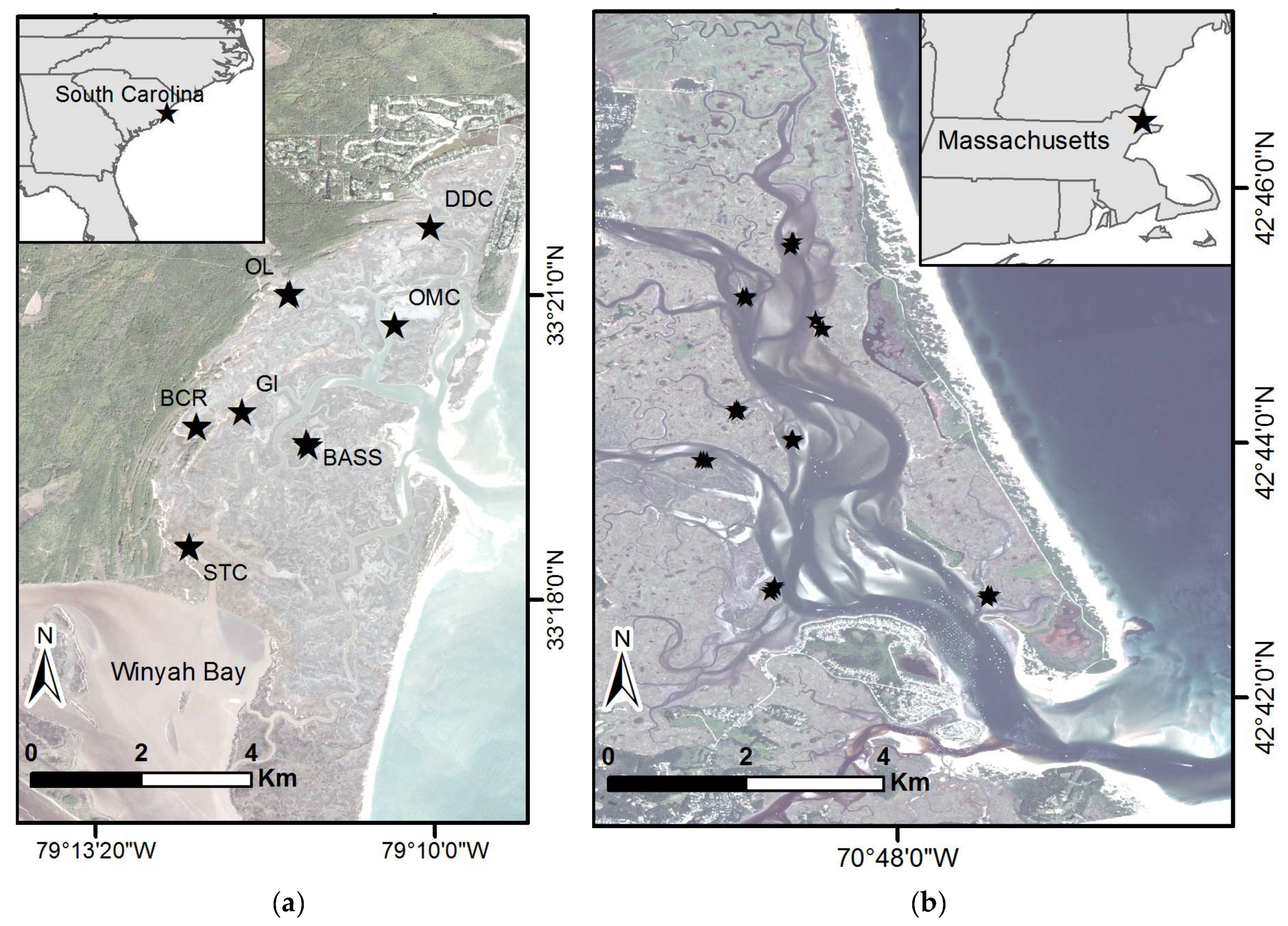
The main study area was North Inlet, in Georgetown, South Carolina (Figure 1a). North Inlet has been the site of multidisciplinary ecological research for about 50 years. The intertidal marshes here consist of 29 km2 of monospecific stands of Spartina alterniflora punctuated by about 121 km of creeks. S. alterniflora possesses long-lived, perennial rhizomes that produce a new crop of stems annually. The mild winters allow for year-round growth, though growth of the newly emergent crop of stems is greatly reduced until milder, brighter conditions prevail in springtime and summer.
Studies of primary production that begun in 1984 at North Inlet documented that interannual anomalies in mean sea level (MSL) on the order of 5 to 10 cm positively affected the productivity of S. alterniflora [19,20]. The effect on plant growth is thought to be due to variations in the duration (hydroperiod) and frequency of tidal flooding, which are determined largely by the marsh elevation relative to mean high water level (MHW). Primary production in the upper quadrant of the tidal frame (roughly the highest 25% of the intertidal zone) is greater in years of high sea level. This is key to the survival of marshes, because the vegetation traps more sediment and generates greater biovolume when greater flood frequency and duration enhance vegetative growth [6].
A smaller study was conducted at the PIE, located in northeastern Massachusetts (Figure 1b). PIE consists of a linked watershed–marsh–estuarine system located within the Boston metropolitan area of northeastern Massachusetts. The brackish and saline tidal wetlands of the PIE site form the major portion of the “Great Marsh”, the largest intact marsh left on the northeast coast of the United States. The coastal ecosystems of PIE are in an area that is changing rapidly. Over the last 30 years, surface sea water temperatures in the Gulf of Maine have risen at 3 times the global average; over the last decade warming has increased 7-fold to 0.23 °C per year, making the Gulf of Maine one of the fastest warming regions in the global ocean [21]. The warming is also associated with a shift in the Gulf Stream that affects local sea level. This area is experiencing high rates of sea-level rise that appear to have accelerated over the last 15 years to nearly 4 mm/year compared to the long-term average of 2.8 mm/year over the last century [22]. PIE is dominated by Spartina patens at high elevations within the tidal frame and S. alterniflora growing at the lower elevations, especially along the creek banks. The cold winters lead to a short growing season, roughly May–August. For this study, only S. alterniflora areas were examined at both North Inlet and PIE.
In addition to climate, major differences between the two sites include tide range and soils. PIE marshes are built on a low-grade peat, while North Inlet marshes rest on mineral sediment. Tide range averages 2.7 m at PIE and 1.4 m at North Inlet [9,23]. The relative elevation of the marsh within the tidal frame, meaning the vertical position between the low- and high-tide levels, is critically important to the resilience of these ecosystems, because it determines their ability to maintain elevation relative to sea level within a favorable vertical range. Spartina marshes exist approximately between mean high water (MHW) and MSL [24], and the biomass of the vegetation is dependent on relative elevation [6]. Thus, theory predicts that biomass should vary across a marsh landscape as a function of elevation. Our analysis of high-resolution data from Planet provided a test of this theory.
2.2. Field Data Collection
For North Inlet, biomass samples were collected at seven sites in each of two years, September 2017 and September 2018. At each site, four sample locations were randomly selected; in total, 54 biomass samples were collected (Figure 1a). These sites were selected because they are accessible and have nearby established sediment elevation tables (SET). A SET is a portable, mechanical leveling device designed to attach to a stable benchmark pipe for the purpose of measuring change in marsh surface elevation [25,26]. Established site names are: DDC—Debidue Creek, OL—Oyster Landing, GI—Goat Island, BASS—Sixty Bass Creek, OMC—Old Man Creek, BCR—Bly Creek, and STC—South Town Creek. For PIE, biomass samples were collected at nine sites during July 2018. Similarly, three to four sample locations were randomly selected and a total of 36 biomass samples were collected. Only areas with monocultures of S. alterniflora were sampled (Figure 1b). At both North Inlet and PIE, a 25 cm × 25 cm quadrat was placed over the plants and plant matter was clipped to the soil surface, excluding fallen litter. The plants were bagged and returned to the laboratory where samples were washed and dried in an oven at 60 °C for 72 h, or until a constant weight was reached. GPS measurements were taken over mudflat locations in North Inlet (12 locations) and PIE (7 locations) to better establish the zero biomass records.
For validation, biomass data collected at North Inlet during monthly surveys at established survey locations were used. This independent dataset is part of a long-term study of biomass production within North Inlet, and is described by Morris and Haskin [19]. Standing biomass was estimated nondestructively by measuring stem heights, and calculating stem weights based on an established empirical relationship [19,27]. Only biomass data from locations that were far enough from the creek edge were used, to avoid interference from water with the spectral data. Biomass values were averaged if multiple sample locations fell within the same pixel, which resulted in a collection of 26 pixel-wise points for model validation in this study.
2.3. Satellite Data
The downloaded PlanetScope images data were acquired on dates close to field sample dates subject to cloud-free and low-tide conditions. For North Inlet, those were 30 October 2017 and 20 September 2018. For PIE, data were collected on 20 July 2018. Planet provided atmospherically corrected multispectral data using the second simulation of a satellite signal in the solar spectrum (6S) radiative transfer model, as has been used successfully in other wetland studies [28,29,30]. The atmospheric correction process uses information from moderate-resolution imaging spectroradiometer (MODIS) for ozone, water vapor, and aerosol inputs [31]. Greater detail about Planet’s sensor specifications is given in Table 1.
2.4. Vegetation Indicies
For each Planet image, the vegetation indices (VI) shown in Table 2 were calculated. The normalized difference vegetation index (NDVI) is a commonly used index measuring plant greenness, with larger values closer to 1.0 indicating the maximum amount of vegetation [32]. Its first salt marsh application was possibly by Hardisky et al. [33] who used a handheld sensor in a Delaware marsh. Background absorption (and reflectance) from soil can have a significant effect on the reflected light, and to account for soil influencing the VI, an adjustment factor (L) is sometimes incorporated into the NDVI calculation resulting the soil adjusted vegetation index (SAVI). Factor L can range from 0 to 1 where 0 indicates complete vegetation coverage and no background effects from soil [34]. An L value of 0.5 minimizes soil brightness variations and is commonly used, but L is based on the amount of vegetation coverage within the study area. Building upon SAVI, the modified soil adjusted vegetation index 2 (MSAVI2) uses a functional L factor that eliminates the need to estimate vegetation density [35]. The renormalized difference vegetation index (RDVI) is an index that reduces oversaturation issues that can be associated with densely vegetated areas [36]. Next, the visible difference vegetation index (VDVI) was originally developed for unmanned aerial systems to highlight plant greenness and uses only values in the visible spectrum [37], and the green normalized vegetation index (GNDVI) can be more sensitive to chlorophyll than NDVI [38]. At each of the field sample locations, we extracted the VI values and surface reflectance from each of the four individual bands and fitted each of these models to square-root normalized biomass.
2.5. Statistical Analysis
The R statistical program was used to run a stepwise method of multiple regression models and determine the best-fit model [39]. The model was initially built using the following formula or a subset of it:
where β0 is the intercept and each subsequent β of 1–10 is the fitted coefficient related to the input variables. Symbols blue, green, red, and NIR represent surface reflectance in each corresponding spectral band. Within R, only models that passed the assumption of non-collinearity were considered.
To normalize the data, the biomass in Equation (1) was input as the square root of field-measured biomass (g/m2). Furthermore, biomass was regressed against the original VIs as well as the logged VIs; the indices can saturate at higher biomass values following a logged shaped curve. We created and compared models with all combinations of vegetation indices and individual spectral bands against each other and selected the best-fit regressions.
This study adopted the Akaike information criterion (AIC) analysis for model comparison. AIC estimates the quality of a model relative to the other models within an analysis, with the smallest AIC model being the best. This allowed us to compare each model against each other by assessing their AIC values and AIC weights (AICw). The AICw calculates the weight of evidence for one model over another model and is calculated based on the entire series of linear regressions in the analysis. The summation of AICw values is 1, which makes for easier model comparison [40]. The AIC values and AIC weights (AICw) can be calculated as [40,41]:
where K is the number of parameters in the model, L is the maximum likelihood function of the model, and is the AIC value for the model minus the AIC value of the smallest model. The model with the lowest AIC and highest AICw is the best model at predicting aboveground biomass.
Three evaluation metrics were examined for performance assessment of the regression model, which was computed using back-transformed output values (biomass g/m2). Its accuracy was quantified using Willmott’s index of agreement (d) [42], which was calculated using the hydroGOF package in R [43]. The index of agreement ranges from 0 to 1, with 1 indicating a perfect fit, and has been used in several remote sensing studies for accuracy assessment [44,45,46,47]. Squared Willmott’s index of agreement (d2) was also included since its values are more similar to the frequently used coefficient of determination (R2) values [48]. Lastly, root mean square error (RMSE) was calculated as:
where n is the number of validation samples, Bobs is the observed biomass (g/m2), and Bmod is the modeled biomass (g/m2).
3. Results
3.1. North Inlet
The regression model that best predicted aboveground biomass (AICw = 0.3848, d = 0.74) was:
In AIC analysis, more dependent variables are counted against the model fit, as shown in Equation (2), and some of the variables such as MSAVI2 and SAVI were autocorrelated, violating the assumption of non-multicollinearity. Therefore, within our analysis, only models with one or two variables were the best-supported models. In Table 3, we include models that showed the most support from our analysis as indicated by an AICw greater than 0.
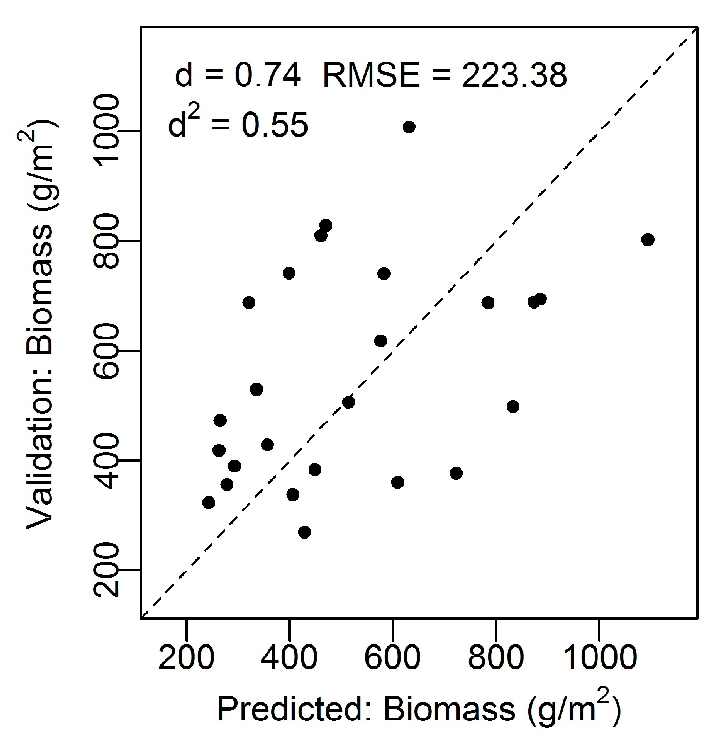
The model accuracy was tested using the independent biomass dataset and there was a good model fit; d = 0.74, d2 = 0.55, n = 26, RMSE = 223.38 g/m2 (Figure 2). The modeled (predicted) values versus the actual values from the validation dataset followed a linear trend that did not significantly deviate from the 1:1 line. Furthermore, the index of agreement was not far from 1 (d = 0.74), indicating a good model fit. The root mean square error (RMSE) of the validation dataset was 223.38 g/m2.
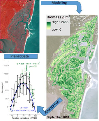
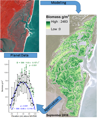
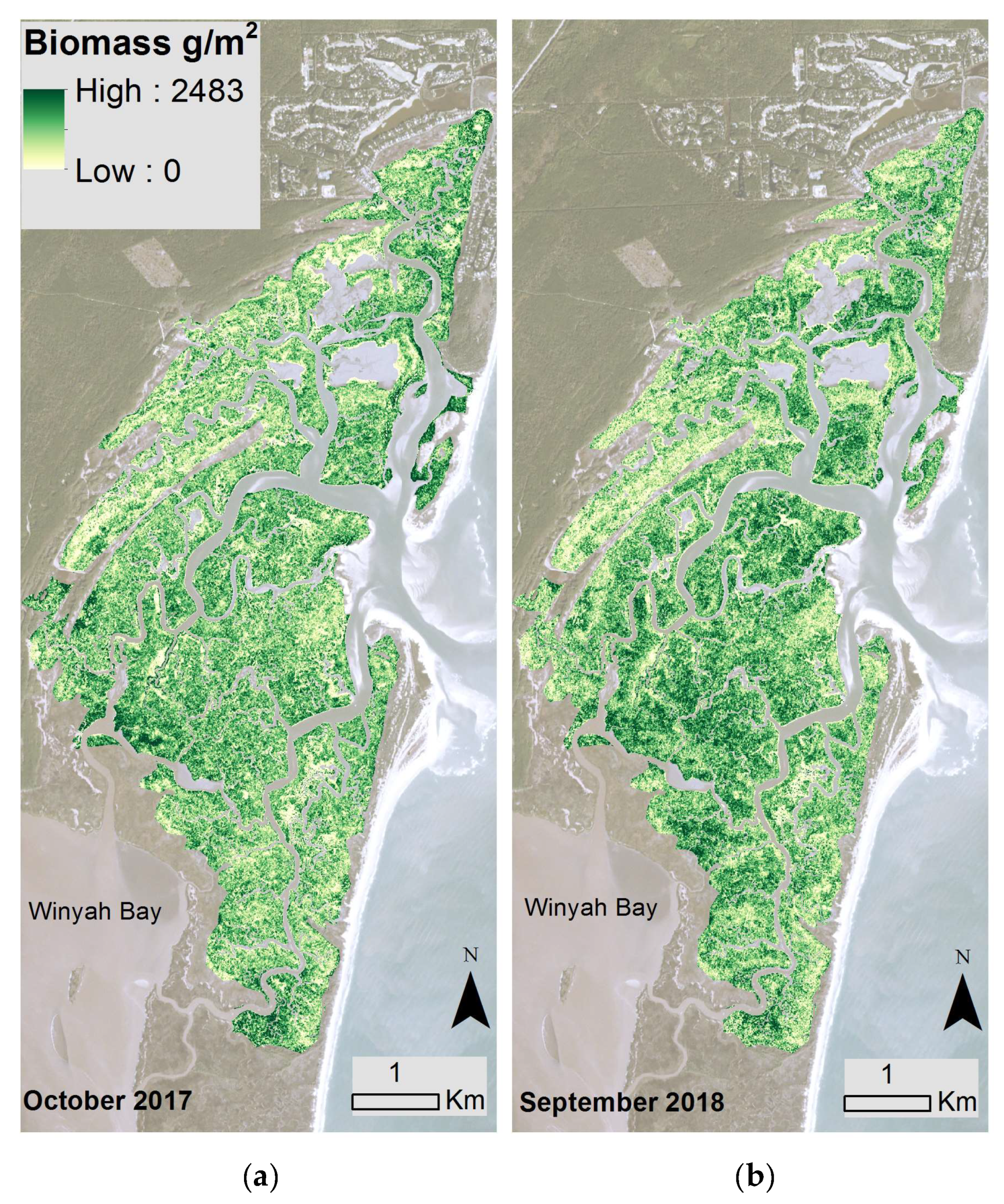
Using the best-fitting model and Planet spectral 3-m data, North Inlet biomass maps were created for 2017 (Figure 3a) and 2018 (Figure 3b). Total aboveground, S. alterniflora biomass across the entire marsh landscape in North Inlet was estimated to be 3423 Mg in 2017 and 2655 Mg in 2018. The maximum area-specific aboveground biomass was 2483 g/m2 and 1823 g/m2 in 2017 and 2018, respectively (Figure 4). The locations of biomass maxima differed between 2017 and 2018. Thus, in addition to interannual temporal variability in the standing crop, there was interannual spatial variability as well, most likely due to varying environmental conditions. To further investigate how biomass differed between the seven locations, modeled biomass values were extracted from 100-m buffers around the sample locations. Most locations had a wide range of biomass, with DDC having a relatively small range. In 2017, BASS had the largest mean biomass and BCR had the lowest (Figure 4). In 2018, DDC had the largest mean biomass and GI had the lowest (Figure 4).
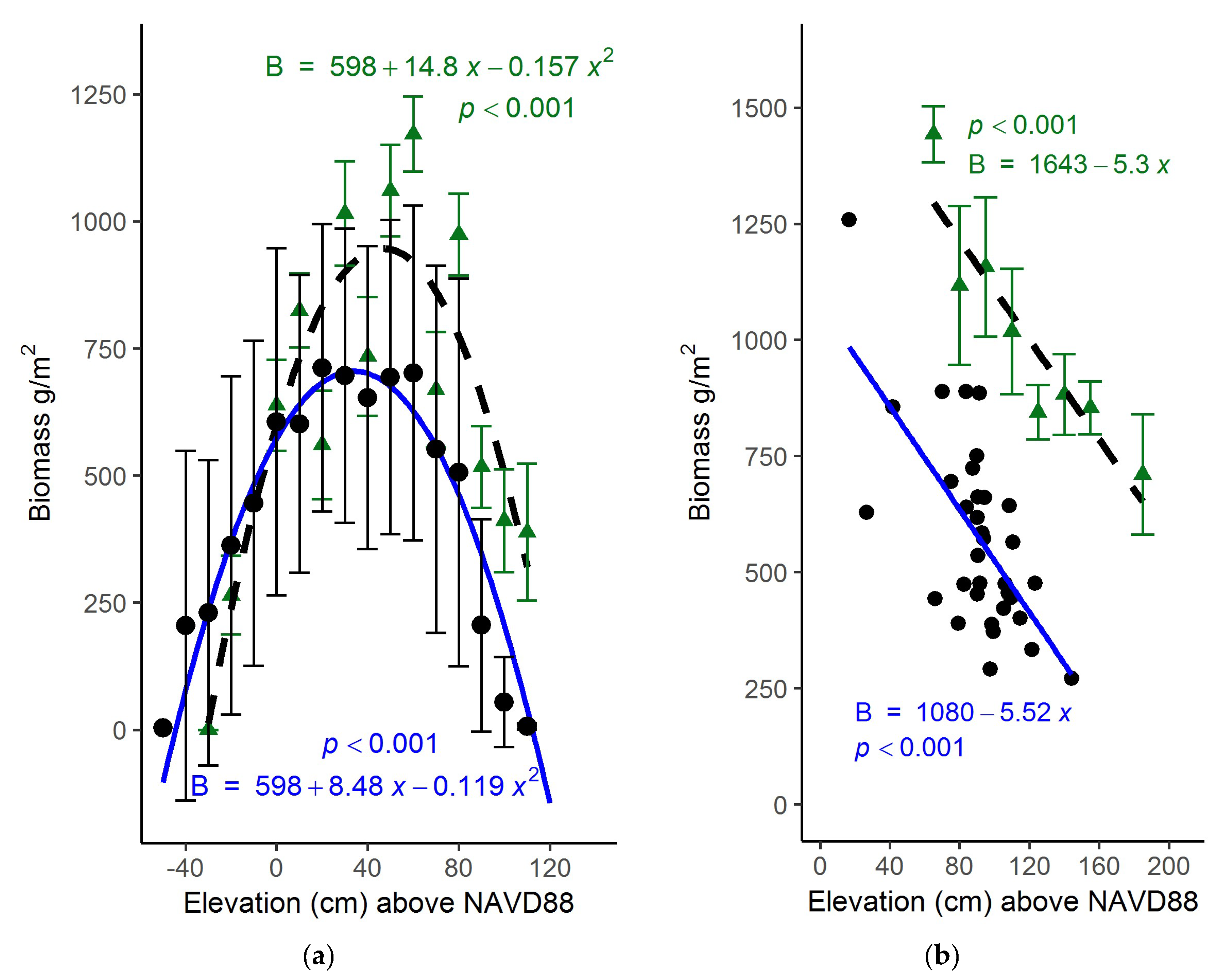
The dependence of biomass on elevation was examined using the model-derived aboveground biomass data (Figure 4) and a 2007 bare-earth lidar-derived digital elevation model. Across the entire marsh landscape, 3000 points were randomly sampled from both the 2017 and 2018 datasets. Using the geolocation of each point, the georeferenced elevation and modeled biomass data were matched. Modelled biomass demonstrated a highly significant parabolic relationship to elevation, with peak biomass near 36 cm above NAVD88 (Figure 5a; p < 0.001). This relationship to elevation was very close to that observed earlier (Figure 5a) in a bioassay experiment in North Inlet [9].
3.2. Plum Island
Harvested aboveground biomass at PIE, like North Inlet, was dependent on elevation (Figure 5b). However, the relationship was linear, which was the case both with the harvest data from this study and a bioassay conducted earlier [9]. The decline in biomass with elevation suggests that the S. alterniflora marshes at PIE occupy the upper half of their possible growth range, at least among the sites we sampled. Unlike PIE, at North Inlet we found S. alterniflora across its entire growth range.
The application of multispectral data in this study for biomass predictions at PIE was less than satisfactory. For example, model Equation (5) fitted to the PIE data showed low model performance d = 0.22 and d2 = 0.05, indicating that Equation (5) might be site-specific and cannot be applied across dissimilar sites. None of the other models were satisfactory either. Additionally, the two vegetation indices MSAVI2 and VDVI, which were used in Equation (5), did not show a relationship with normalized biomass (Figure 6).
4. Discussion
Planet data were applied successfully to estimate aboveground biomass at North Inlet. A good model fit (d = 0.74, d2 = 0.55, RMSE = 223.38 g/m2) was obtained using the model developed within this study to estimate biomass at the validation sites. The extracted biomass map provided interesting insights about this marsh’s growth dynamics that correlated well with data from marsh organ studies, including correspondence with the vertical growth ranges.
Within North Inlet we found that mean biomass varied by sample location. As indicated in Figure 4, differences in biomass density were significant due to variable growth conditions within the estuary. STC had the largest biomass concentration and is also the location closest to Winyah Bay. Winyah Bay is an estuary adjacent to North Inlet (Figure 3) with a large freshwater discharge, and its adjacent marshes are less saline than the majority of North Inlet estuary. The water from Winyah Bay only influences the southern region of North Inlet, due to a tidal node that limits the intrusion of brackish water further into North Inlet [23]. STC was the only site we sampled that was influenced by Winyah Bay, and the freshwater influence presumably provided for more favorable growth conditions, allowing for larger biomass growth.
There are other sources of variation that have not been fully explained. For instance, total biomass in 2017 was greater than in 2018, however it is unclear what led to this change. The images used in 2017 and 2018 both were taken at low tide (−0.5 m and −0.42 m relative to NAVD, respectively) and in the same season, so influences of tide and time-of-year were minimal. However, it is possible that atmospheric conditions differed between images and were not perfectly or uniformly corrected using atmospheric correction. Alternatively, rainfall may have been a factor [19,30]. Based on the Palmer drought severity index for the northeast region in South Carolina, 2017 experienced more “incipient wet spells during the growing season than in 2018, which should have been more favorable for growth. Then in February/March of 2018 there was a period of “mild drought” (Figure 7) [49,50], which likely depressed growth. Although there was no notable prolonged drought in 2018, the average summer temperature was slightly cooler in 2017 and springtime wetter than 2018, both of which may have resulted in somewhat more favorable 2017 growing conditions (Figure 8). Other factors that influence aboveground biomass include herbivory, interannual variation in sea level, and storms [19,30,51,52,53]. Thus, the remote imagery has opened up future work on the possible drivers of these inter-annual differences in marsh primary production.
Elevation also played a role in biomass growth, and similar to other studies, biomass followed a parabolic relationship with elevation [6,9,54]. Furthermore, the biomass curve closely follows the curve found in a marsh organ experiment conducted at North Inlet and PIE [9]. The comparison of results from this study and that of the marsh organ study (shown in Figure 5a,b) demonstrates that PlanetScope data are useful in deriving biomass growth curves, and can be an alternative to labor-intensive, in situ bioassay experiments. Though the overall harvested biomass at PIE was lower than what was found in a PIE marsh organ experiment, perhaps due to time of harvest, the slope of the two growth curves were similar. For North Inlet, the peak biomass is at mid elevations within its vertical range. As noted earlier, the optimal elevation for S. alterniflora growth is approximately midway between mean sea level and the level of mean higher high water [9], which is presumably the least stressful elevation [6]. This is consistent with our biomass model and supports that Planet data or alternative remote imagery can be utilized to derive a relationship between elevation and biomass production based on vegetation indices and a DEM. This would expand the utility of predictive models such as MEM and allow for better predictions of marsh survival and migration in the face of rising sea level.
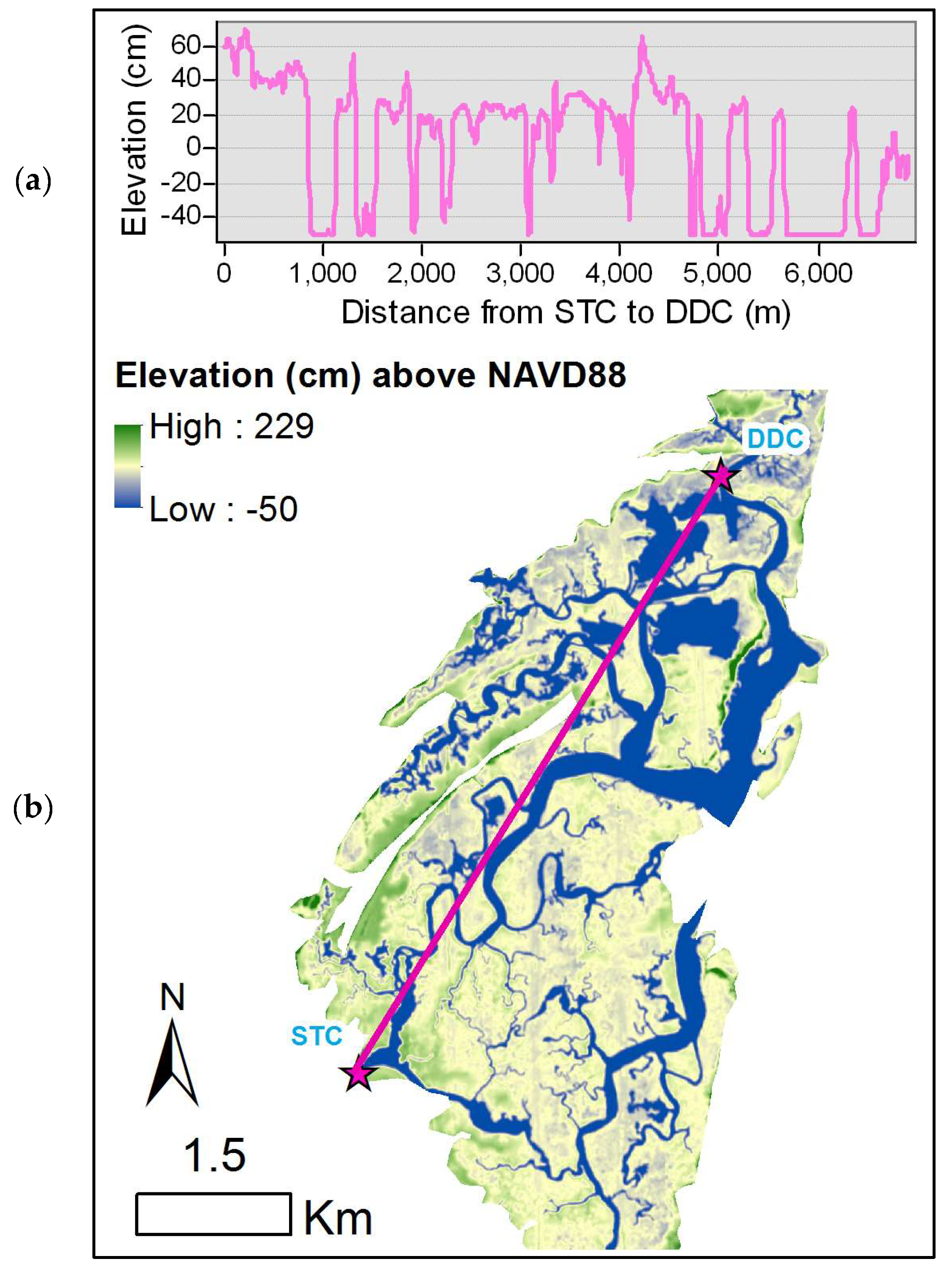
There is a north-south elevation gradient within North Inlet (Figure 9a,b) that may also influence the biomass. As noted above, there are differences in biomass among sample sites, and the mosaic of biomass (Figure 3) clearly shows a preponderance of high biomass at the south end of North Inlet. The elevation at that end of the estuary (Figure 9) is close to the optimum (Figure 5), while elevations at the north end are suboptimal. Consequently, marsh areas at the north end are at greater risk of drowning due to sea-level rise.
The sample size for PIE was possibly too small to realize a significant correlation between the spectral data and aboveground biomass. Another factor may have been the dark organic-rich soils that are characteristic of PIE marshes. Further, based on field observations, biomass, plant form, and stem density at PIE are extremely variable. For instance, biomass was over 160 cm tall at one site and under 20 cm at another. The issues of large biomass variance and possible spectral saturation with tall dense vegetation at PIE could potentially have been overcome using a larger sample size. In addition, a better correlation between satellite data and biomass may have been established if S. patens samples had been included, but the architecture of the two species is radically different. To maintain consistency across sites, only S. alterniflora was included. Future work should be conducted at PIE to include more plant species, larger sample size, and a wider growth range.
The biomass density observed at PIE in this study was lower than what was found in a marsh organ study (Figure 5b), although the trends with elevation were the same, confirming that growth of S. alterniflora varies with elevation. However, the growth curves for North Inlet and PIE were different (Figure 5). Within PIE, S. alterniflora growth is largely confined to the higher end of its growth range. Moreover, as noted earlier, the tide range at PIE is greater than at North Inlet. Consequently, the potential or fundamental vertical growth range of S. alterniflora is greater at PIE than at North Inlet. However, S. alterniflora’s realized growth range in North Inlet spans the entirety of its fundamental range, which our data fully captured, which is possibly another reason for the model’s success at North Inlet and failure at PIE.
Biomass and satellite data from PIE were collected earlier in the annual growth cycle than at North Inlet, which also may have affected the fidelity of the models because the spectral signature of S. alterniflora varies throughout the year [55,56]. Satellite and field data for PIE were collected in July while samples were collected in North Inlet during early autumn. The growing season also differs between the two sites, as discussed above. Therefore, the spectral signatures of PIE and North Inlet plants were likely very different, which would lead to differences in vegetation indices values. To better determine if a universal biomass model using Planet or other spectral data could be used, future work should match field and satellite data during peak VI values at each sample site.
This study supports the use of small satellites as a reliable platform to provide data that may be used to compute and map marsh biomass. The commonly applied medium-resolution data such as Landsat is less helpful since the fine-scale spatial variability of marsh biomass is smoothed in those images. As one example of the rapidly developing small satellite technologies, PlanetScope have data originating in 2009. However, their target for near-daily data was reached in 2017. Planet continues to launch their PlanetScope satellites several times a year ridesharing with other missions. These low-cost small satellites have a lifespan of about three years, which allows the company to update the satellite’s hardware. The low cost and frequent launch of new satellites also reduces the cost risk of a failed mission. An added benefit of PlanetScope data is that the satellites are always in operation, while other high-resolution satellites are often task-based. This feature provides PlanetScope users with high spatial and temporal coverage of data. Data accessibility is an issue. Since Planet is a commercial company, its data are not as easily accessible as NASA’s frequently used Landsat data. In addition, taken with frame cameras, the radiometric accuracy of Planet data may not be as high as that of Landsat. However, this has not yet been widely studied. Despite these drawbacks, the high spatial resolution and temporal frequency of PlanetScope makes it especially useful within heterogeneous wetland systems that are influenced by tides and summer cloud covers.
5. Conclusions
This study successfully utilized Planet multispectral data to create 3-m spatial scale resolution maps within the North Inlet Winyah Bay National Estuarine Research Reserve. The derived model cannot universally be applied to all wetlands, such as the Plum Island Ecosystems Long-Term Ecological Research site, however this may have been due to differences in season and small sample size, among other possibilities. The advantage of using Planet’s data is its high spatial resolution and repeat time, which allows for analysis of biomass distribution and temporal change on a finer scale. The finer scale analysis is particularly useful for land and coastal managers interested in assessing marsh health. Furthermore, the frequent repeat time of Planet’s satellite series provides more usable coastal data; analysis within a salt marsh requires imagery collected during low tide, and clouds often cover the coast during the summer making it difficult to find suitable data.
Pairing the model-derived landscape scale map with elevation data, a robust biomass curve with elevation was established. This is important for establishing a better understanding of factors that control biomass growth and is an important input to biogeomorphic models of marsh response to rising sea level. This study not only highlights the usefulness of a newer satellite sensor, but also shows how high-resolution satellite-derived products help answer questions about spatial variability within a marsh and overall marsh condition.
Author Contributions
Conceptualization, G.J.M. and J.T.M.; methodology, G.J.M. and C.W.; software, G.J.M.; validation, G.J.M.; formal analysis, G.J.M.; investigation, G.J.M., J.T.M., and C.W.; resources, J.T.M.; data curation, G.J.M.; writing—original draft preparation, G.J.M.; writing—review and editing, J.T.M. and C.W.; visualization, G.J.M.; supervision, J.T.M.; project administration, G.J.M.; funding acquisition, J.T.M. and G.J.M.
Funding
This research was funded by NSF grants LTREB-654853 and OCE-1637630, the Slocum-Lunz Foundation, and the F. John Vernberg Bicentennial Fellowship.
Acknowledgments
We would like to thank Karen Sundberg for help with fieldwork.
Conflicts of Interest
The authors declare no conflict of interest.
References
- Möller, I.; Kudella, M.; Rupprecht, F.; Spencer, T.; Paul, M.; van Wesenbeeck, B.K.; Wolters, G.; Jensen, K.; Bouma, T.J.; Miranda-Lange, M.; et al. Wave attenuation over coastal salt marshes under storm surge conditions. Nat. Geosci. 2014, 7, 727–731. [Google Scholar] [CrossRef] [Green Version]
- Narayan, S.; Beck, M.W.; Wilson, P.; Thomas, C.J.; Guerrero, A.; Shepard, C.C.; Reguero, B.G.; Franco, G.; Ingram, J.C.; Trespalacios, D. The Value of Coastal Wetlands for Flood Damage Reduction in the Northeastern USA. Sci. Rep. 2017, 7, 9463. [Google Scholar] [CrossRef] [PubMed]
- Fisher, J.; Acreman, M. Wetland nutrient removal: a review of the evidence. Hydrol. Earth Syst. Sci. 2004, 8, 673–685. [Google Scholar] [CrossRef] [Green Version]
- Nellemann, C.; Corcoran, E.; Duarte, C.M.; Valdés, L.; De Young, C.; Fonseca, L.; Grimsditch, G. Blue Carbon—The Role of Healthy Oceans in Binding Carbon; United Nations Environment Programme, GRID-Arendal: Nairobi, Kenya, 2009; ISBN 9788277010601. [Google Scholar]
- Mcleod, E.; Chmura, G.L.; Bouillon, S.; Salm, R.; Björk, M.; Duarte, C.M.; Lovelock, C.E.; Schlesinger, W.H.; Silliman, B.R. A blueprint for blue carbon: toward an improved understanding of the role of vegetated coastal habitats in sequestering CO2. Front. Ecol. Environ. 2011, 9, 552–560. [Google Scholar] [CrossRef]
- Morris, J.T.; Sundareshwar, P.V.; Nietch, C.T.; Kjerfve, B. Responses of Coastal Wetlands to Rising Sea Level. Ecol. Soc. Am. 2002, 83, 2869–2877. [Google Scholar] [CrossRef]
- DeLaune, R.D.; Smith, C.J.; Patrick, W.H. Relationship of Marsh Elevation, Redox Potential, and Sulfide to Spartina alterniflora Productivity1. Soil Sci. Soc. Am. J. 1983, 47, 930. [Google Scholar] [CrossRef]
- Miller, G.J.; Morris, J.T.; Wang, C. Mapping salt marsh dieback and condition in South Carolina’s North Inlet-Winyah Bay National Estuarine Research Reserve using remote sensing. AIMS Environ. Sci. 2017, 4, 677–689. [Google Scholar] [CrossRef]
- Morris, J.T.; Sundberg, K.; Hopkinson, C.S. Salt Marsh Primary Production and Its Response to Relative Sea Level and Nutrients in Estuaries at Plum Island, Massachusets, and North Inlet, South Carolina, USA. Oceanography 2013, 26, 78–84. [Google Scholar] [CrossRef]
- Silliman, B.R.; Bertness, M.D. A trophic cascade regulates salt marsh primary production. Proc. Natl. Acad. Sci. USA 2002, 99, 10500–10505. [Google Scholar] [CrossRef] [Green Version]
- Mendelssohn, I.A. Nitrogen Metabolism in the Height Forms of Spartina Alterniflora in North Carolina. Ecology 1979, 60, 574–584. [Google Scholar] [CrossRef]
- Mendelssohn, I.A.; Seneca, E.D. The influence of soil drainage on the growth of salt marsh cordgrass Spartina alterniflora in North Carolina. Estuar. Coast. Mar. Sci. 1980. [Google Scholar] [CrossRef]
- Gross, M.F.; Klemas, V.; Hardisky, M.A. Long-term remote monitoring of salt marsh biomass. Remote Sens. Biosph. 1990, 1300, 59–70. [Google Scholar]
- Lumbierres, M.; Méndez, P.; Bustamante, J.; Soriguer, R.; Santamaría, L. Modeling Biomass Production in Seasonal Wetlands Using MODIS NDVI Land Surface Phenology. Remote Sens. 2017, 9, 392. [Google Scholar] [CrossRef]
- Gross, M.F.; Hardisky, M.A.; Klemas, V.; Wolf, P.L. Quantification of Biomass of the Marsh Grass Spartina altfernifara Loisel Using Landsat Thematic Mapper Imagery. Photogramm. Eng. Remote Sens. 1987, 53, 1577–1583. [Google Scholar]
- Mo, Y.; Kearney, M.S.; Riter, J.C.A. Post-deepwater horizon oil spill monitoring of Louisiana salt marshes using landsat imagery. Remote Sens. 2017, 9, 547. [Google Scholar] [CrossRef]
- Lopes, C.L.; Mendes, R.; Caçador, I.; Dias, J.M. Evaluation of long-term estuarine vegetation changes through Landsat imagery. Sci. Total Environ. 2019, 653, 512–522. [Google Scholar] [CrossRef] [PubMed]
- Planet Team Planet Application Program Interface: In Space for Life on Earth. Available online: https://api.planet.com/ (accessed on 2 December 2018).
- Morris, J.T.; Haskin, B. A 5-yr Record of Aerial Primary Production and Stand Characteristics of Spartina Alterniflora. Ecology 1990, 71, 2209. [Google Scholar] [CrossRef]
- Morris, J.T. Effects of sea-level anomalies on estuarine processes. In Estuarine Science: A Synthetic Approach to Research and Practice; Hobbie, J.E., Ed.; Island Press: Washington, DC, USA, 2000; pp. 107–127. [Google Scholar]
- Pershing, A.J.; Alexander, M.A.; Hernandez, C.M.; Kerr, L.A.; Le Bris, A.; Mills, K.E.; Nye, J.A.; Record, N.R.; Scannell, H.A.; Scott, J.D.; et al. Slow adaptation in the face of rapid warming leads to collapse of the Gulf of Maine cod fishery. Science 2015, 350, 809–812. [Google Scholar] [CrossRef] [Green Version]
- NOAA Boston Tide Gage, Tides & Currents. Available online: https://tidesandcurrents.noaa.gov/stationhome.html?id=8443970 (accessed on 30 July 2019).
- Schwing, F.B.; Kjerfve, B.; Kjerfve, B. Longitudinal Characterization of a Tidal Marsh Creek Separating Two Hydrographically Distinct Estuaries. Estuaries 1980, 3, 236. [Google Scholar] [CrossRef]
- McKee, K.L.; Patrick, W.H. The Relationship of Smooth Cordgrass (Spartina alterniflora) to Tidal Datums: A Review. Estuaries 1988, 11, 143. [Google Scholar] [CrossRef]
- Cahoon, D.R.; Lynch, J.C.; Hensel, P.; Boumans, R.; Perez, B.C.; Segura, B.; Day, J.W. High-Precision Measurements of Wetland Sediment Elevation: I. Recent Improvements to the Sedimentation-Erosion Table. J. Sediment. Res. 2002, 72, 730–733. [Google Scholar] [CrossRef]
- Boumans, R.M.J.; Day, J.W. High Precision Measurements of Sediment Elevation in Shallow Coastal Areas Using a Sedimentation-Erosion Table. Estuaries 1993, 16, 375. [Google Scholar] [CrossRef]
- Davis, J.; Currin, C.; Morris, J.T. Impacts of Fertilization and Tidal Inundation on Elevation Change in Microtidal, Low Relief Salt Marshes. Estuaries and Coasts 2017, 40, 1677–1687. [Google Scholar] [CrossRef]
- Byrd, K.B.; O’Connell, J.L.; Di Tommaso, S.; Kelly, M. Evaluation of sensor types and environmental controls on mapping biomass of coastal marsh emergent vegetation. Remote Sens. Environ. 2014, 149, 166–180. [Google Scholar] [CrossRef]
- Li, W.; Gong, P. Continuous monitoring of coastline dynamics in western Florida with a 30-year time series of Landsat imagery. Remote Sens. Environ. 2016, 179, 196–209. [Google Scholar] [CrossRef]
- O’Donnell, J.; Schalles, J.; O’Donnell, J.P.R.; Schalles, J.F. Examination of Abiotic Drivers and Their Influence on Spartina alterniflora Biomass over a Twenty-Eight Year Period Using Landsat 5 TM Satellite Imagery of the Central Georgia Coast. Remote Sens. 2016, 8, 477. [Google Scholar] [CrossRef]
- Planet Team Planet Imagery Product Specification. Available online: https://assets.planet.com/docs/combined-imagery-product-spec-final-may-2019.pdf (accessed on 20 May 2019).
- Rouse, J.W.; Hass, R.H.; Schell, J.A.; Deering, D.W. Monitoring vegetation systems in the great plains with ERTS. In Proceedings of the Third Earth Resources Technology Satellite (ERTS) symposium, Washington, DC, USA, 10–14 December; pp. 309–317.
- Hardisky, M.A.; Smart, R.M.; Klemas, V. Seasonal Spectral Characteristics and aboveground Biomass of the Tidal Marsh Plant, Spartina alterniflora. Photogramm. Eng. Remote Sens. 1983, 49, 85–92. [Google Scholar]
- Huete, A. A soil-adjusted vegetation index (SAVI). Remote Sens. Environ. 1988, 25, 295–309. [Google Scholar] [CrossRef]
- Qi, J.; Chehbouni, A.; Huete, A.R.; Kerr, Y.H.; Sorooshian, S. A Modified Soil Adjusted Vegetation Index. Remote Sens. Environ. 1994, 48, 119–126. [Google Scholar] [CrossRef]
- Roujean, J.-L.; Breon, F.-M. Estimating PAR absorbed by vegetation from bidirectional reflectance measurements. Remote Sens. Environ. 1995, 51, 375–384. [Google Scholar] [CrossRef]
- Wang, X.; Wang, M.; Wang, S.; Wu, Y. Extraction of vegetation information from visible unmanned aerial vehicle images. Trans. Chinese Soc. Agric. Eng. 2015, 31, 152–159. [Google Scholar]
- Gitelson, A.A.; Merzlyak, M.N. Remote sensing of chlorophyll concentration in higher plant leaves. Adv. Space Res. 1998, 22, 689–692. [Google Scholar] [CrossRef]
- R Core Team R. A Language and Environment for Statistical Computing; R Foundation for Statistical Computing: Vienna, Austria, 2017. [Google Scholar]
- Burnham, K.P.; Anderson, D.R. Model Selection and Multimodel Inference: A Practical Information-Theoretic Approach; Springer Science & Business Media: Berlin/Heidelberg, Germany, 2002; ISBN 0387953647. [Google Scholar]
- Akaike, H. A new look at the statistical model identification. IEEE Trans. Automat. Contr. 1974, 19, 716–723. [Google Scholar] [CrossRef]
- Willmott, C.J. Some Comments on the Evaluation of Model Performance. Bull. Am. Meteorol. Soc. 1982, 63, 1309–1313. [Google Scholar] [CrossRef] [Green Version]
- Zambrano-Bigiarini, M. hydroGOF: Goodness-of-fit functions for comparison of simulated and observed hydrological time series. Available online: http://hzambran.github.io/hydroGOF/ (accessed on 21 June 2019).
- Hardisky, M.A.; Daiber, F.C.; Roman, C.T.; Klemas, V. Remote sensing of biomass and annual net aerial primary productivity of a salt marsh. Remote Sens. Environ. 1984, 16, 91–106. [Google Scholar] [CrossRef]
- Yebra, M.; Chuvieco, E. Linking ecological information and radiative transfer models to estimate fuel moisture content in the Mediterranean region of Spain: Solving the ill-posed inverse problem. Remote Sens. Environ. 2009, 113, 2403–2411. [Google Scholar] [CrossRef]
- García, M.; Riaño, D.; Chuvieco, E.; Danson, F.M. Estimating biomass carbon stocks for a Mediterranean forest in central Spain using LiDAR height and intensity data. Remote Sens. Environ. 2010, 114, 816–830. [Google Scholar] [CrossRef]
- de Almeida, D.R.A.; Nelson, B.W.; Schietti, J.; Gorgens, E.B.; Resende, A.F.; Stark, S.C.; Valbuena, R. Contrasting fire damage and fire susceptibility between seasonally flooded forest and upland forest in the Central Amazon using portable profiling LiDAR. Remote Sens. Environ. 2016, 184, 153–160. [Google Scholar] [CrossRef]
- Valbuena, R.; Hernando, A.; Manzanera, J.A.; Görgens, E.B.; Almeida, D.R.A.; Silva, C.A.; García-Abril, A. Evaluating observed versus predicted forest biomass: R-squared, index of agreement or maximal information coefficient? Eur. J. Remote Sens. 2019, 52, 1–14. [Google Scholar] [CrossRef]
- Palmer, W.C. Meteorological drought. Res. Pap. 1965, 45, 58. [Google Scholar]
- NOAA National Climatic Data Center. Available online: https://www7.ncdc.noaa.gov/CDO/CDODivisionalSelect.jsp# (accessed on 26 May 2019).
- Dame, R.F.; Kenny, P.D. Variability of Spartina alterniflora primary production in the euhaline North Inlet estuary. Mar. Ecol. Prog. Ser. 1986, 32, 71–80. [Google Scholar] [CrossRef]
- Tyler, A.C.; Zieman, J.C. Patterns of development in the creekbank region of a barrier island Spartina alterniflora marsh. Mar. Ecol. Prog. Ser. 1999, 180, 161–177. [Google Scholar] [CrossRef] [Green Version]
- Li, S.; Pennings, S.C. Timing of disturbance affects biomass and flowering of a saltmarsh plant and attack by stem-boring herbivores. Ecosphere 2017, 8, e01675. [Google Scholar] [CrossRef]
- Walters, D.C.; Kirwan, M.L. Optimal hurricane overwash thickness for maximizing marsh resilience to sea level rise. Ecol. Evol. 2016, 6, 2948–2956. [Google Scholar] [CrossRef] [PubMed] [Green Version]
- Ouyang, Z.-T.; Gao, Y.; Xie, X.; Guo, H.-Q.; Zhang, T.-T.; Zhao, B. Spectral Discrimination of the Invasive Plant Spartina alterniflora at Multiple Phenological Stages in a Saltmarsh Wetland. PLoS ONE 2013, 8, e67315. [Google Scholar] [CrossRef] [PubMed]
- Jialin, L.; Hanbing, Z.; Xiaoping, Y. Study on the seasonal dynamics of zonal vegetation of NDVI/EVI of costal zonal vegetation based on MODIS data: A case study of Spartina alterniflora salt marsh on Jiangsu Coast, China. Afr. J. Agric. Res. 2011, 6, 4019–4024. [Google Scholar]
Figure 1.
Study areas and sample sites, with stars indicating sample locations. (a) North Inlet-Winyah Bay National Estuarine Research Reserve within South Carolina. Established sample locations names are: DDC—Debidue Creek, OL—Oyster Landing, GI—Goat Island, BASS—Sixty Bass Creek, OMC—Old Man Creek, BCR—Bly Creek, STC—South Town Creek. (b) Study site at the Plum Island Ecosystems Long-Term Ecological Research site within Massachusetts. Basemap images courtesy of Planet Labs, Inc. (San Francisco, CA, USA).

Figure 2.
Modeled biomass (g/m2) from the combined modified soil vegetation index 2 (MSAVI2) and visible difference vegetation index (VDVI) versus the validation biomass (g/m2) data. Dashed line corresponds to the 1:1 line indicating a perfect match between the measured and predicted values. Root mean square error (RMSE) = 223.38 g/m2, Willmott’s index of agreement (d) = 0.74, and squared Willmott’s index of agreement (d2) = 0.55.

Figure 3.
Modeled biomass from the back-transformation of Equation (2) across the marsh landscape at North Inlet from Planet satellite data acquired in (a) October 2017 and (b) September 2018. Basemap images courtesy of Planet Labs, Inc.
Figure 3.
Modeled biomass from the back-transformation of Equation (2) across the marsh landscape at North Inlet from Planet satellite data acquired in (a) October 2017 and (b) September 2018. Basemap images courtesy of Planet Labs, Inc.

Figure 4.
Whisker and box plot of field-collected biomass samples within North Inlet. Top and bottom of the boxes indicate the third and first quartile, respectively. Horizontal line within the box indicates the median value and the whiskers indicate the maximum and minimum.
Figure 4.
Whisker and box plot of field-collected biomass samples within North Inlet. Top and bottom of the boxes indicate the third and first quartile, respectively. Horizontal line within the box indicates the median value and the whiskers indicate the maximum and minimum.
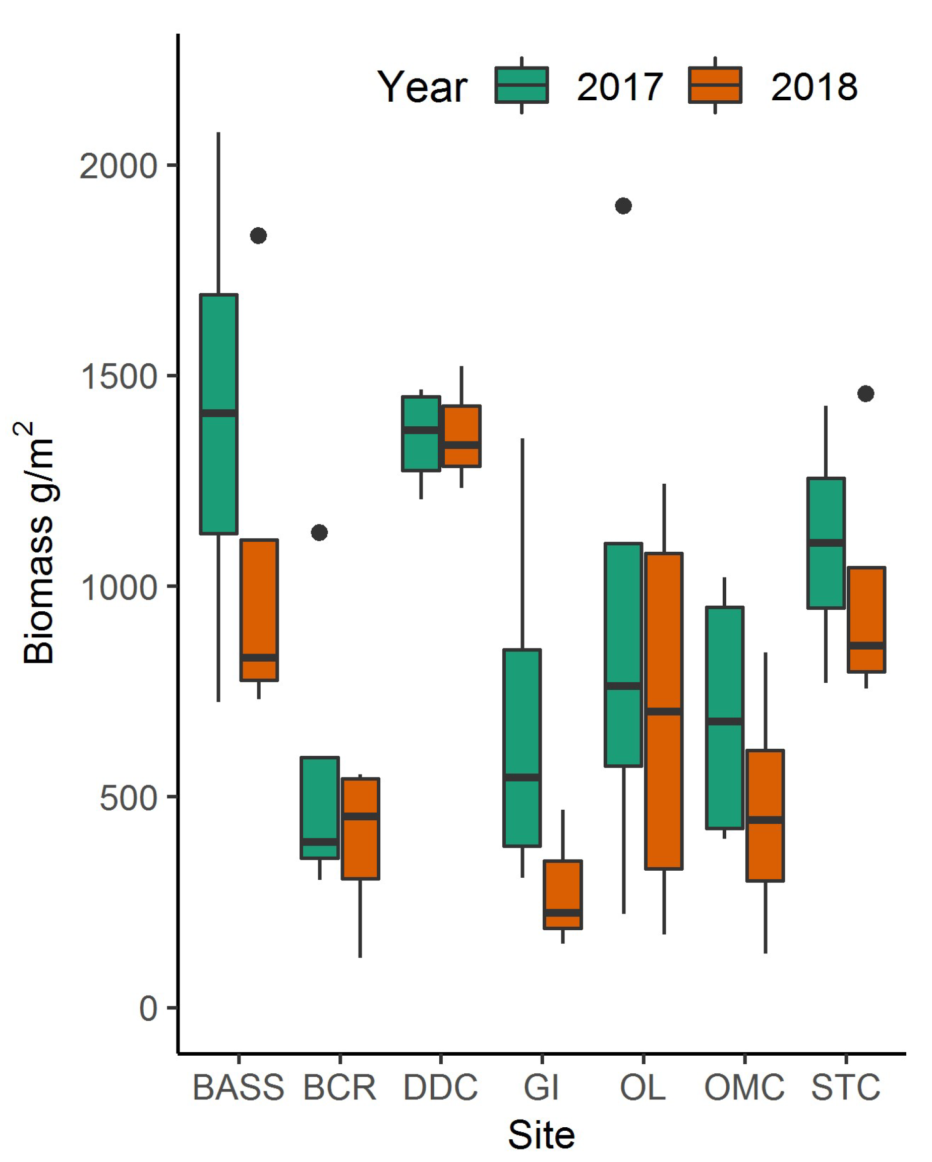
Figure 5.
Aboveground biomass (g/m2) versus plot elevation (cm) above NAVD88 within North Inlet and PIE. (a) North Inlet—shown in black are the means (±1 SD) of calculated biomass found at North Inlet across a range of elevations modelled using Equation (2). Biomass predictions shown here were back-transformed by squaring the model calculation. The blue line is a least-squares fit of a parabola (p < 0.001) to these data. Shown in green are the means (±1 SE) from a North Inlet marsh-organ experiment [9] and the least-squares best fit of a parabola. (b) PIE—black circles are (June) harvested biomass samples from this study collected in salt marshes dominated by Spartina alterniflora. The blue regression line indicates dependence of field collected biomass (g/m2) on elevation (cm). Green triangles are means (±1 SE) of end-of-season biomass from in PIE marsh organ experiment [9] with dashed linear regression line.

Figure 6.
Square-root biomass g/m2 plotted against vegetation indexes within PIE. (a) Visible differences vegetation index (VDVI); (b) modified soil vegetation index 2 (MSAVI2).
Figure 6.
Square-root biomass g/m2 plotted against vegetation indexes within PIE. (a) Visible differences vegetation index (VDVI); (b) modified soil vegetation index 2 (MSAVI2).
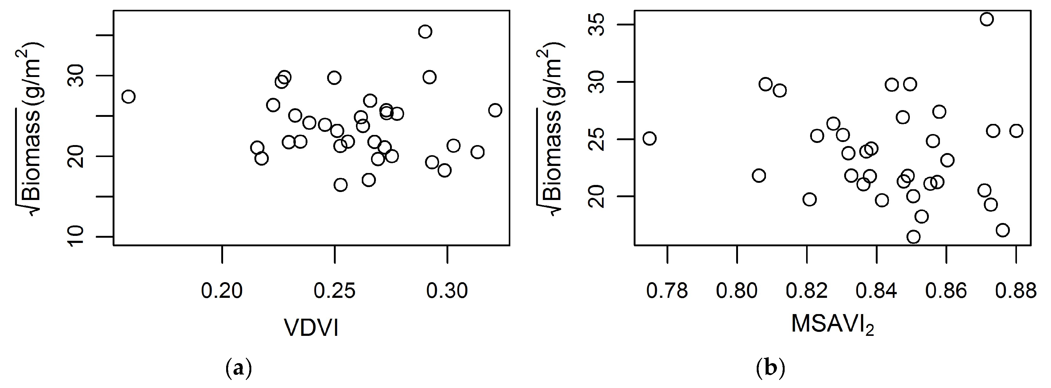
Figure 7.
Palmer drought severity index for the Northeast South Carolina region. This region encompasses North Inlet. Negative values indicate drought and positive values indicate wet periods. Values between 0.5 and 1 indicate “inceptive wet periods,” values between 1 and 2 indicate slightly wet, values between −0.5 and −1 indicate incipit dry spells, and values between −1 and −2 indicate mild drought.
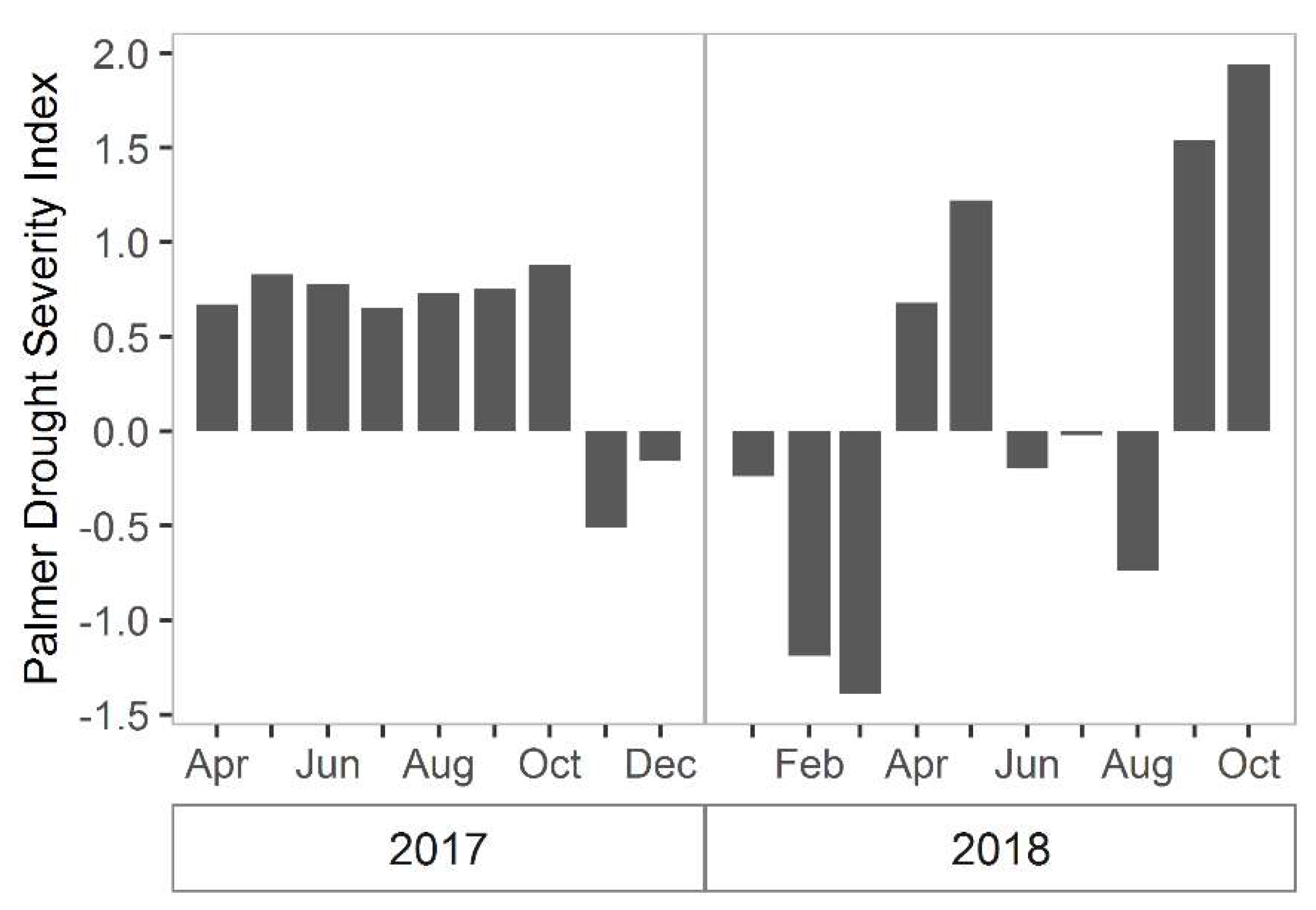
Figure 8.
Average monthly temperature (°C) and cumulative monthly precipitation during the growing season within North Inlet for 2017 and 2018. The bar graph indicates precipitation and line graph indicates temperature. Data are from a weather station at North Inlet.
Figure 8.
Average monthly temperature (°C) and cumulative monthly precipitation during the growing season within North Inlet for 2017 and 2018. The bar graph indicates precipitation and line graph indicates temperature. Data are from a weather station at North Inlet.
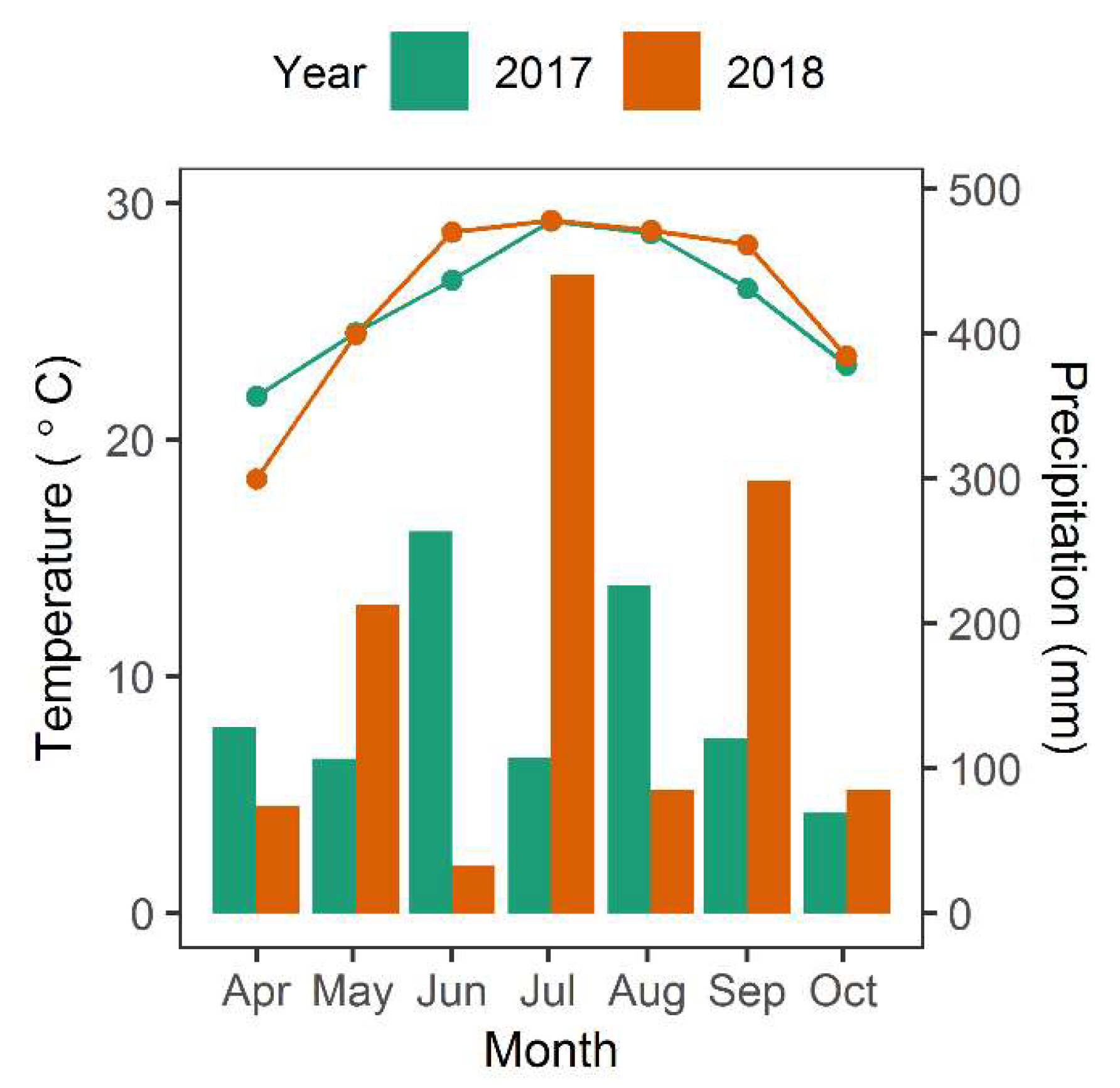
Figure 9.
Elevation within North Inlet: (a) Elevation profile across the estuary from the southernmost sample site (STC) to the northernmost site (DDC) and (b) elevation (cm) above NAVD88 with a pink line representing the transect shown in (a).
Figure 9.
Elevation within North Inlet: (a) Elevation profile across the estuary from the southernmost sample site (STC) to the northernmost site (DDC) and (b) elevation (cm) above NAVD88 with a pink line representing the transect shown in (a).


Table 1.
Summary of PlanetScope sensor characteristics.
| Characteristic | Value |
|---|---|
| Blue wavelength (nm) | 455–415 |
| Green wavelength (nm) | 500–590 |
| Red wavelength (nm) | 590–670 |
| NIR wavelength (nm) | 780–860 |
| Spatial Resolution (m) | 3 × 3 |
| Temporal Resolution | Near daily |
| Image size (km) | 24 × 7 |
Table 2.
Vegetation indices and the associated formulas used in the analysis.
| Vegetation Index | Equation | Reference |
|---|---|---|
| NDVI | [32] | |
| SAVI 1 | [34] | |
| MSAVI2 | [35] | |
| RDVI | [36] | |
| VDVI | [37] | |
| GNDVI | [38] |
1 L is a soil adjustment factor ranging from 0 to 1, with 0 indicating no background effect from soil. A frequently used value is 0.5, which was adopted in this study.
Table 3.
All models were fitted to square-root normalized aboveground biomass. The model with the highest Akaike information criterion (AIC) weight (AICw) is the best model. The table only included models that had an AICw larger than 0.
Table 3.
All models were fitted to square-root normalized aboveground biomass. The model with the highest Akaike information criterion (AIC) weight (AICw) is the best model. The table only included models that had an AICw larger than 0.
| Model | AIC | AICw |
|---|---|---|
| (MSAVI2) + (VDVI) | 364.4 | 0.3848 |
| MSAVI2 + VDVI | 365.2 | 0.2636 |
| SAVI + VDVI | 365.6 | 0.2122 |
| VDVI + GNDVI | 367.3 | 0.0856 |
| VDVI | 370.4 | 0.0231 |
| (B3) + (VDVI) | 371.8 | 0.0096 |
| B3 + (VDVI) | 372.3 | 0.0073 |
| MSAVI2 + B3 | 372.6 | 0.0064 |
| (MSAVI2) + (B3) | 373.3 | 0.0045 |
| SAVI + NDVI | 374.5 | 0.0025 |
| MSAVI2 | 382.4 | 0.0001 |
© 2019 by the authors. Licensee MDPI, Basel, Switzerland. This article is an open access article distributed under the terms and conditions of the Creative Commons Attribution (CC BY) license (http://creativecommons.org/licenses/by/4.0/).
Share and Cite
MDPI and ACS Style
Miller, G.J.; Morris, J.T.; Wang, C. Estimating Aboveground Biomass and Its Spatial Distribution in Coastal Wetlands Utilizing Planet Multispectral Imagery. Remote Sens. 2019, 11, 2020. https://doi.org/10.3390/rs11172020
AMA Style
Miller GJ, Morris JT, Wang C. Estimating Aboveground Biomass and Its Spatial Distribution in Coastal Wetlands Utilizing Planet Multispectral Imagery. Remote Sensing. 2019; 11(17):2020. https://doi.org/10.3390/rs11172020
Chicago/Turabian StyleMiller, Gwen J., James T. Morris, and Cuizhen Wang. 2019. "Estimating Aboveground Biomass and Its Spatial Distribution in Coastal Wetlands Utilizing Planet Multispectral Imagery" Remote Sensing 11, no. 17: 2020. https://doi.org/10.3390/rs11172020
Note that from the first issue of 2016, this journal uses article numbers instead of page numbers. See further details here.