The Impacts of Growth and Environmental Parameters on Solar-Induced Chlorophyll Fluorescence at Seasonal and Diurnal Scales

Abstract

Solar-induced chlorophyll fluorescence (SIF) is considered to be a potential indicator of photosynthesis. However, the impact of growth and environmental parameters on SIF at different time-scales remains unclear, which has greatly restricted the application of SIF in detecting photosynthesis variations. Thus, in this study, the impact of growth and environmental parameters on SIF was thoroughly clarified. Here, continuous time series of canopy SIF (760 nm, F760) over wheat and maize was measured based on an automated spectroscopy system. Meanwhile, field measurements of growth and environmental parameters were also collected using commercial-grade devices. Relationships of these parameters with F760, apparent SIF (F760/solar radiance, AF760), and SIF yield (F760/canopy radiance of 685 nm, Fy760) were analyzed using principal component analysis (PCA) and Pearson correlation to reveal their impacts on SIF. Results showed that F760 at seasonal and diurnal scales were mainly driven by solar radiation (SWR), leaf area index (LAI), chlorophyll content (Chl), mean leaf inclination angle (MTA), and relative water content (RWC). Other environmental parameters, including air temperature (Ta), relative humidity (Rh), vapor pressure deficit (VPD), and soil moisture (SM), contribute less to the variation of seasonal or diurnal F760. AF760 and Fy760 are likely to be less dependent on Ta, Rh, and VPD due to the removal of the impact from SWR, but an enhanced relationship of AF760 (and Fy760) with SM was observed, particularly under water stress. Compared with F760, wheat AF760 was better correlated to LAI and RWC as expected, while maize AF760 did not show an enhanced relationship with all growth parameters, probably due to its complicated canopy structure. The relationship of wheat Fy760 with canopy structure parameters was further reduced, except for maize measurements. Furthermore, SM-induced water stress and phenological stages should be taken into consideration when we interpret the seasonal and diurnal patterns of SIF since they were closely related to photosynthesis and plant growth (e.g., LAI in our study). To our knowledge, this is the first exploration of the impacts of growth and environmental parameters on SIF based on continuous ground measurements, not only at a seasonal scale but also at a diurnal scale. Our results could provide deep insight into the variation of SIF signals and also promote the further application of SIF in the health assessments of terrestrial ecosystems.

1. Introduction

Solar-induced chlorophyll fluorescence (SIF) is an optical signal that is emitted by chlorophyll a molecules when absorbed solar energy exceeds the requirements of the photochemical reaction [1]. It has attracted the attention of botanists, ecologists, and agricultural scientists since SIF gives an insight into the photosynthetic machinery of terrestrial vegetation [2]. However, it is difficult to decouple SIF from reflected solar flux, which is mainly due to the much lower contribution of SIF emission to the reflected signal (1–5% in the near-infrared) [3]. In order to overcome this problem, the in-filling method using two dark bands in telluric oxygen (O₂) absorption lines (O₂-A, 760 nm and O₂-B, 687 nm) has commonly been used for SIF retrieval because of the more comparable signal of SIF relative to reflected flux in these two O₂ bands [3,4]. These two O₂ bands are also close to the terrestrial SIF spectrum peaks centered at ≈685 and ≈740 nm, known as red and far-red fluorescence [5]. While the O₂-B band coincides almost entirely with the red fluorescence, its depth is much lower and width is much smaller than that of the O₂-A band [6]. Therefore, the O₂-A band has largely been used to estimate SIF from tower [7,8,9], aircraft [10,11], and satellite platforms [12,13,14,15].

It has been demonstrated that SIF can be considered as a potential indicator of photosynthesis at different scales. It was reported that, at the leaf and canopy level of crops, relative SIF (the ratio of SIF and radiance at O₂ band) is inversely related to photosynthetic light-use efficiency (LUE), and the correlation of SIF with LUE is better at 760 nm than that at 687 nm [16]. At regional scales, the apparent SIF yield (SIF is divided by incident photosynthetically active radiation) also correlates well with the maximum carboxylation rate (Vcmax), a key parameter of leaf biological traits [17]. These results provide us with further understanding about global photosynthesis, which drives the global carbon cycle and fixes carbon dioxide (CO₂) as organic compounds [18]. This carbon flux at the ecosystem level is known as gross primary production (GPP) [19], which plays an important role in the global food security and carbon budgets [20]. In recent studies, a strong linear relationship was found between SIF and GPP in specific ecosystem types [21,22,23], suggesting that SIF could serve as a good proxy for GPP estimation. Moreover, early information of stress-induced changes in photosynthesis could also be detected by the measurements of SIF on the ground [7,10] or from space [12,14,15]. Therefore, it might be concluded that SIF could provide accurate and more direct information for functional status of vegetation, carbon assimilation estimate, and stress detection over large scales [24].

Although the feasibility of SIF in these above aspects has been widely discussed, it remains challenging to use SIF as a direct indicator of photosynthesis due to the fact that some growth and environmental parameters could also affect SIF emissions at different time scales. For example, solar radiation is a critical environmental parameter that drives the variation of SIF at seasonal and diurnal scales [9,25]. Air temperature and vapor pressure deficit (VPD) also affect the seasonal patterns of SIF over different land covers [9,12,26] and exhibit different relationships with SIF under the influence of water stress [10]. SIF also shows a great sensitivity to growth parameters, such as chlorophyll content, leaf area index, and leaf inclination angles, because these parameters could affect the absorption of solar energy and ultimately result in the variation of LUE in the end [10,27,28]. Different plant types and phenological stages could also induce the variation of growth parameters and thus cause the difference of SIF emissions [27,29,30]. Most of these findings were separately explored at different spatio-temporal scales over different vegetation types and commonly based on simulated results [31]. Few studies were conducted to simultaneously assess their impacts on SIF, especially based on the continuous ground measurements over various types of plant. Meanwhile, the relationship of SIF yield (and apparent SIF yield), a more direct signal of photosynthesis than SIF, with these parameters has never been reported using ground measurements. Thus, further work needs to be carried out to bridge the gap toward the correct interpretation of the SIF signal in the sequential application for the health assessment of a terrestrial ecosystem.

In order to compare and analyze the impacts of growth and environmental parameters on SIF (including SIF, SIF yield, and apparent SIF yield), high-frequency time series of canopy SIF over four plots of wheat and maize were collected in 2017 (from 28 March to 19 May for wheat and 29 July to 28 September for maize) with an automated observation system. Environmental parameters including solar radiation, air temperature, and relative humidity were collected from a nearby micro-meteorological station. Canopy structure (leaf area index and mean leaf inclination angle) and leaf physiological parameters (chlorophyll content and leaf water content) were also collected during the field campaign. With these measurements, we aimed to address the following questions: (1) How does the SIF of wheat and maize change at seasonal and diurnal scales? (2) What is the detailed relationship between SIF and each environmental or biophysical parameter? Answers to these questions can provide deep understanding about the effect of environmental and biophysical parameters on SIF variations, both at seasonal and diurnal scales. This paper is structured as follows: Section 2 describes the experimental design, the measurements of environmental and growth parameters, the spectrum collection method, and data processing. The results and discussions are detailed in Section 3 and Section 4, respectively. Finally, Section 5 provides the conclusions.

2. Materials and Methods

Experimental design over wheat and maize are described in Section 2.1, including field plot design, planting and harvest time, irrigation strategy, and precipitation during the filed campaigns. The methods used for the collection of growth and environmental parameters are then described in Section 2.2. Then, the details of the methods for spectrum collection and SIF retrieval are introduced in Section 2.3. Finally, the data processing for normalizing SIF is provided in Section 2.4. All measurements over wheat have been previously described in detail [32,33].

2.1. Experimental Design

Winter wheat and summer maize were planted on 20 October 2016 and 20 June 2017 in four 4 m × 4 m plots (Figure 1b,c) at the Fangshan Comprehensive Experimental Station (39°35’N, 115°42.5’E), Beijing Normal University. Field campaigns were separately conducted from March 28 to May 19 of 2017 for wheat and from July 29 to September 29 of 2017 for maize. An irrigation amount of 60 mm was applied to each plot before winter (7 November 2016) to ensure the winter wheat could endure the freezing cold in the winter (the monthly average temperature between November in 2016 and February in 2017 was 1.3 °C). From mid-October of 2016 to late-March in 2017, about 55 mm accumulated precipitations were recorded by a micro-weather station adjacent to the experimental plots (Figure 2a). Without the influence of precipitation on wheat growth after green up (March 28 to May 19 of 2017), different irrigation treatments were applied over four plots of wheat to generate a drought gradient. For plot 4, no irrigation was applied to simulate an extreme drought condition. For the other three plots, different irrigation treatments were conducted four times, separately on 28 March, 22 April, 2 May, and 12 May 2017 (Figure 2b). More in detail, the same volume of irrigation with 60 mm was applied on 28 March over the three plots, while the irrigation amounts in the subsequent three practices were 60, 40, and 25 mm, applied separately to plot 1, plot 2, and plot 3, respectively. For plot 1, the accumulated irrigation was about 300 mm, which could largely satisfy the demand of evapotranspiration during the whole growth season of winter wheat [34,35]. Thus, the wheat in plot 1 was unstressed, while the other three plots were subjected to water stress since their accumulated irrigation was much lower than 300 mm. Furthermore, the intensity of water stress was in an increasing order for plot 2, plot 3, and plot 4. Besides, no irrigation was applied over maize due to the rich precipitation after sowing. As shown in Figure 2a, the accumulated precipitation during the maize growth season was ≈360 mm, which is in the range of the water requirement of summer maize (350–400 mm) [36]. Therefore, maize in our field experiment did not suffer from water stress.

2.2. The Measurements of Environmental and Growth Parameters

Environmental parameters, including solar radiation (SWR, W $·$ m⁻²), air temperature (Ta, °C), relative humid (Rh, recorded as a fraction), and soil moisture (SM, m³/m³), were continuously collected using commercial devices. A data logger (HOBO U30, Onset Computer Corporation, Bourne, MA, USA) in the micro-meteorological station nearby our experimental plots was used to record the real-time values of SWR (300–1100 nm, S-LIB-M003, Onset Computer Corporation), as well as Ta and Rh (S-THB-M002, for Ta and Rh collection, Onset Computer Corporation), with a time interval of 5 min (Figure 1b,c). VPD was further calculated using Ta and Rh according to Equation (1). The values of SM in the soil layer at 20 cm were also collected by soil moisture sensors (S-SMC-M005, Onset Computer Corporation). To obtain high quality measurements of SM, two sensors were equipped in each plot (Figure 1b). Daily means of SM in each plot were averaged from the records of two sensors.

$$\mathrm{VPD}=0.611\times e^{\frac{17.27\times {\mathrm{T}}_{\mathrm{a}}}{{\mathrm{T}}_{\mathrm{a}}+237}}\times \left(1-\mathrm{Rh}\right)$$

(1)

Weekly measurements of growth parameters were conducted over four plots of wheat and maize to analyze their influence on the variation of seasonal and diurnal SIF. These parameters included leaf area index (LAI), mean leaf inclination angle (MTA), chlorophyll content (Chl), and relative leaf water content (RWC). Both LAI and MTA were measured using the LAI-2200c Plant Canopy Analyzer (LI-COR Inc., Lincoln, NE, USA) under low solar irradiance (about 17:00–18:30 for each measurement). Daily LAI (MTA) in each plot was calculated as the average values of three continuous LAI (MTA) measurements over the same plot. Chl values were indicated as SPAD readings, which were collected at noon (12:00–12:30) using a hand-held absorbance-based dualwavelength chlorophyll meter (SPAD-502, Minolta Corporation, Ltd., Osaka, Japan). About 20 leaves were selected as samples for each plot and the averaged value was saved to represent the concentration of Chl. The daily mean of RWC for each plot was averaged from six leaf samples excised at midday (12:30 to 13:30) every time. The excised leaf was weighed immediately and recorded as the fresh weight (FW). Then, the fresh leaf was soaked in distilled water in a test tube for eight hours in darkness. After that, the turgid weight (TW) was obtained by weighting the water-saturated leaves. The leaves were then dried overnight at 80 °C and re-weighed as the dry weight (DW). RWC was calculated according to Equation (2) [37,38]:

$$\mathrm{RWC}=\frac{\mathrm{F}-\mathrm{DW}}{\mathrm{TW}-\mathrm{DW}}$$

(2)

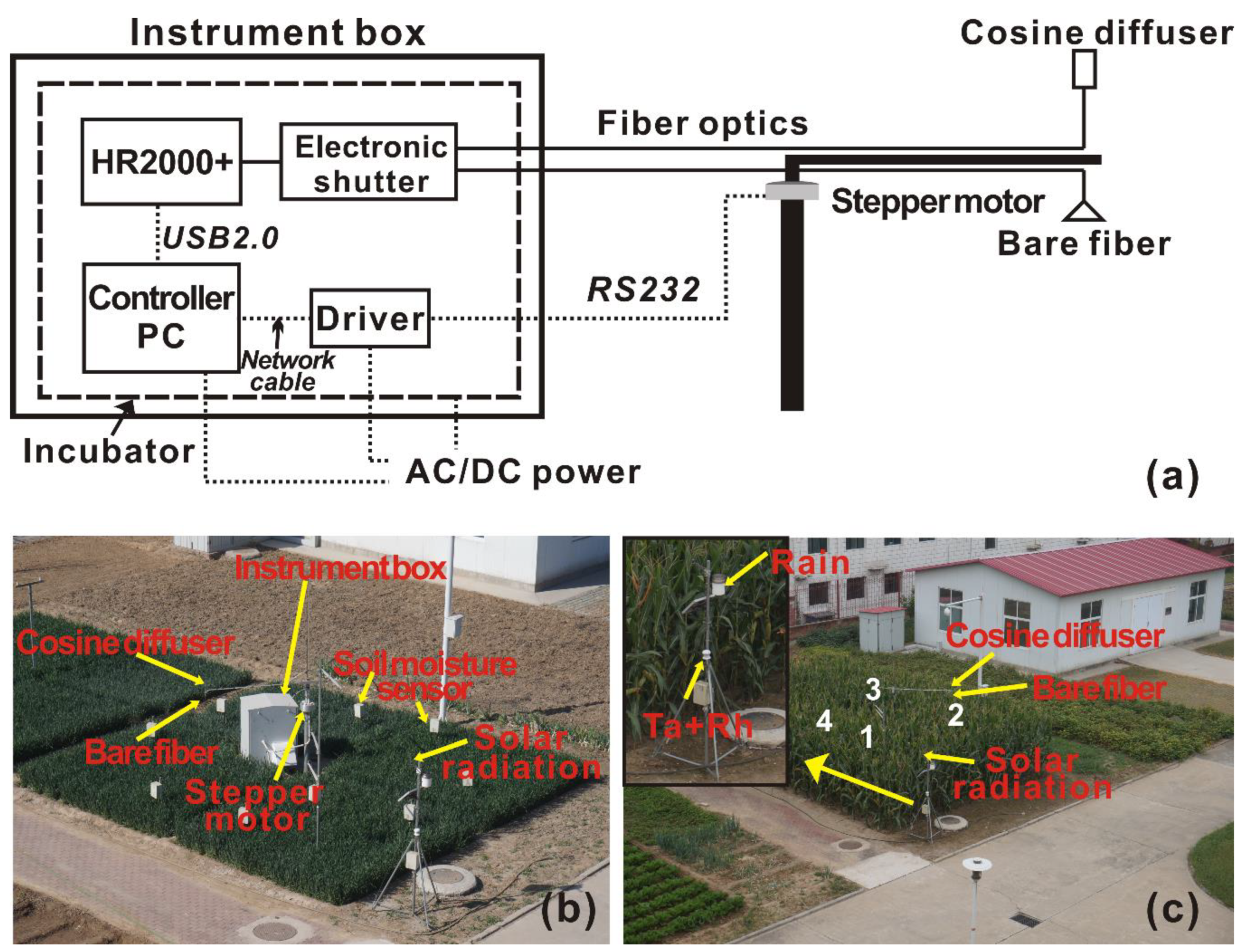
2.3. Automated Field Spectroscopy System and the Measurements of SIF

An automated field spectroscopy system was designed using commercial-grade optoelectronic devices for continuous and simultaneous collection of canopy SIF over the four plots. This platform has been extensively described in Liu et al. [32,33]. The automated system consisted of four key components: one key component is a high-resolution spectrometer HR2000+ (Ocean Optics Inc., Largo, FL, USA), covering the spectral range of 680–775 nm with a spectral resolution of ≈0.13 nm (full width at half maximum, FWHM); the second one is an electronic shutter (FOS-2 x 2-TTL, Ocean Optics Inc.) to connect the spectrometer with a splitter fiber (Ocean Optics Inc.); the third one is two fiber optics that were fixed on a mechanical arm and attached with the electronic shutter; and the fourth key component was a step motor, which was used to drive a mechanical arm from one plot to another one. All devices embedded in the system were connected to a PC through the connection of Universal Serial Bus 2.0 (USB 2.0) or Recommended Standard 232 (RS232). The system was placed in an incubator, where the temperature was kept at 23 °C to reduce the influence of temperature on the dark current of the spectrometer. An instrument box was used to protect these devices from rain.

Solar irradiance and canopy radiance were collected by a custom-developed software. This software was compiled into an executable file in Microsoft Visual Studio 2015 (Microsoft, Redmond, WA, USA) and run under the Microsoft Windows operating system (Windows 7). The Software Development Kit (SDK) in the driver OOIWinIP (OOIDrv32.lib, Ocean Optics Inc.) was used to control HR2000+ and the electronic shutter. Solar irradiance was collected by the up-looking fiber with a cc-3 cosine diffuser (Ocean Optics Inc.) with a field of view (FOV) of 180${}^{°}$, while the up-welling canopy flux was collected from nadir with a down-looking bare fiber with a FOV of 25${}^{°}$ (Figure 1a). The distance between the bare fiber and canopy was greater than 150 cm for wheat during the whole field campaign. However, such a distance for maize was greater than 100 cm before late August; after that, the distance became smaller. These two optical paths could be switched by the electronic shutter that allows only one signal enter the spectrometer at a one time.

In our field campaigns, all the measurements of spectrum were collected during 6:00 to 19:00. In each plot, solar irradiance was first collected through the up-looking fiber, then canopy radiance was collected using the down-looking bare fiber. Solar irradiance and canopy radiance in each plot were collected in five minutes to reduce the impact of short-term changes in illumination conditions.

The dark current with the same integration time as spectra collection (i.e., 2 s, 3 s, or 5 s in our study) was also collected as a digital number (DN) before filed campaigns at the fixed temperature of 23 °C. Dark-current correction was performed according to the method of “raw spectra (DN) – dark current (DN)” to eliminate the impact of the dark current on raw spectra. After that, a second degree polynomial Savitzky-Golay filtering method with a filter of 30 × 30 spectral bands was used to reduce the noise of the raw spectra. We also performed radiometric and wavelength calibrations before filed campaigns two times in the platform of SpectraSuite (Ocean Optics Inc.) by using a radiometric calibration light source (HL-2000-CAL, Ocean Optics Inc.) and a wavelength calibration light source (HG-1, Ocean Optics Inc.). The radiance correction factor and absolute irradiance correction factor were collected using the field calibration. Based on the correction factors, the output raw data were then converted to irradiance (E, mW∙m⁻²∙nm⁻²) and radiance (L, mW∙m⁻²∙nm⁻²∙sr⁻¹).

Before SIF retrieval, data quality was checked to further reject the data affected by short-term changes in illumination conditions, which was similar to the quality evaluation in Cogliati, et al. [25]. First, those data between 8:00 and 17:00 (sun zenith angle was smaller than ≈${60}^{°}$) were selected to conduct the next process. Second, quick-changing solar light was considered as the fraction of variation between the corrected irradiance in one plot (E1) and the irradiance in the next plot (E2), i.e., |E2 − E1|/E1. Those acquired data were rejected when their |E2 − E1|/E1 value was above 0.2. Third, the raw data greater than 15,000 DN were also rejected because of the saturation that occurred in HR2000+. The rapid increase in illumination was also assessed using the ratio of canopy radiance (L) and the corresponding solar irradiance (E/π). The data was also rejected when L/(E/π) was greater than 1. Only those data that satisfied all these quality indicators were used to estimate SIF values at 760 nm (F760). The bands covering the range of 755.6–765.6 nm (242 bands) were used to retrieve SIF by means of spectral fitting methods (SFM) [3]. Both reflectance and SIF were assumed to be linear functions of wavelength. Those SIF data were selected only when the fitting algorithm achieved R² > 0.99.

2.4. Data Processing and Analysis

Apparent SIF yield and SIF yield were always used in most previous relevant literatures to indicate the dynamics of photosynthesis. Their relationships with growth and environmental parameters were also considered in our study. Apparent SIF yield is generally calculated as SIF/PAR, where PAR is the incident photosynthetically active radiation. However, in our study, PAR values were only collected during wheat growth season by using a radiance sensor (S-LIA-M003, Onset Computer Corporation), and unfortunately the records of PAR during maize growth season were missing due to damage to the sensor. Therefore, the ratio of F760/SWR (referred to as AF760 hereafter) was used to represent apparent SIF yield due to the fact that PAR was about 47% of the total incoming solar radiation [26]. For the SIF yield, it could not be calculated according to the commonly used method of SIF/APAR (APAR is the PAR absorbed by canopy), since APAR was not directly collected in our study as well. An alternative method that is expressed as the ratio of F760 to canopy radiance flux at 685 nm (F760/L685, Fy760) was used to represent SIF yield. This method is developed based on the assumption that L685 (radiance near the O₂-B absorption band) is mainly linked to the variation of APAR [39].

Pearson correlation analysis and principal component analysis (PCA) were employed to explore the relationships of F760, AF760, and Fy760 with growth and environmental parameters. Pearson correlation is often used and easily understood, while the PCA method in our study is not easy to understand because the utilized PCA method is mainly used in numerical ecology to indicate the relationship among variables [40,41]. In its application, PCA generally reduces a multidimensional sample space into fewer dimensions (i.e., principal components) by assuming a linear relationship between each dimension with all variables [42]. Results of PCA, including the samples and variables, can be plotted on a two-dimensional PCA projection: a biplot [41]. The biplot not only groups the samples, but also determines relationships between samples and variables. Relationships among variables were indicated by vector angles: if the vector angle between two variables is acute, they are positively correlated; else if the angel is obtuse, these two variables were negatively correlated (the right angle represents uncorrelated) [41]. From the biplot, we can sort out a pattern of variables among the samples and provide relational information about the variables [43]. In our study, we only analyzed relationships between variables. Furthermore, all averaged hourly and daily measurements were used in the analysis of the Pearson correlation and PCA for separately indicating the relationship of SIF with growth and environmental parameters at diurnal and seasonal scales. PCA was performed using the package “vegan” (version 2.5-5, https://mirrors.tuna.tsinghua.edu.cn/CRAN/) of R software (version 3.4.0, https://www.r-project.org/) [44], and the Pearson correlation coefficients (r) were calculated using the R software built-in package “stats”.

3. Results

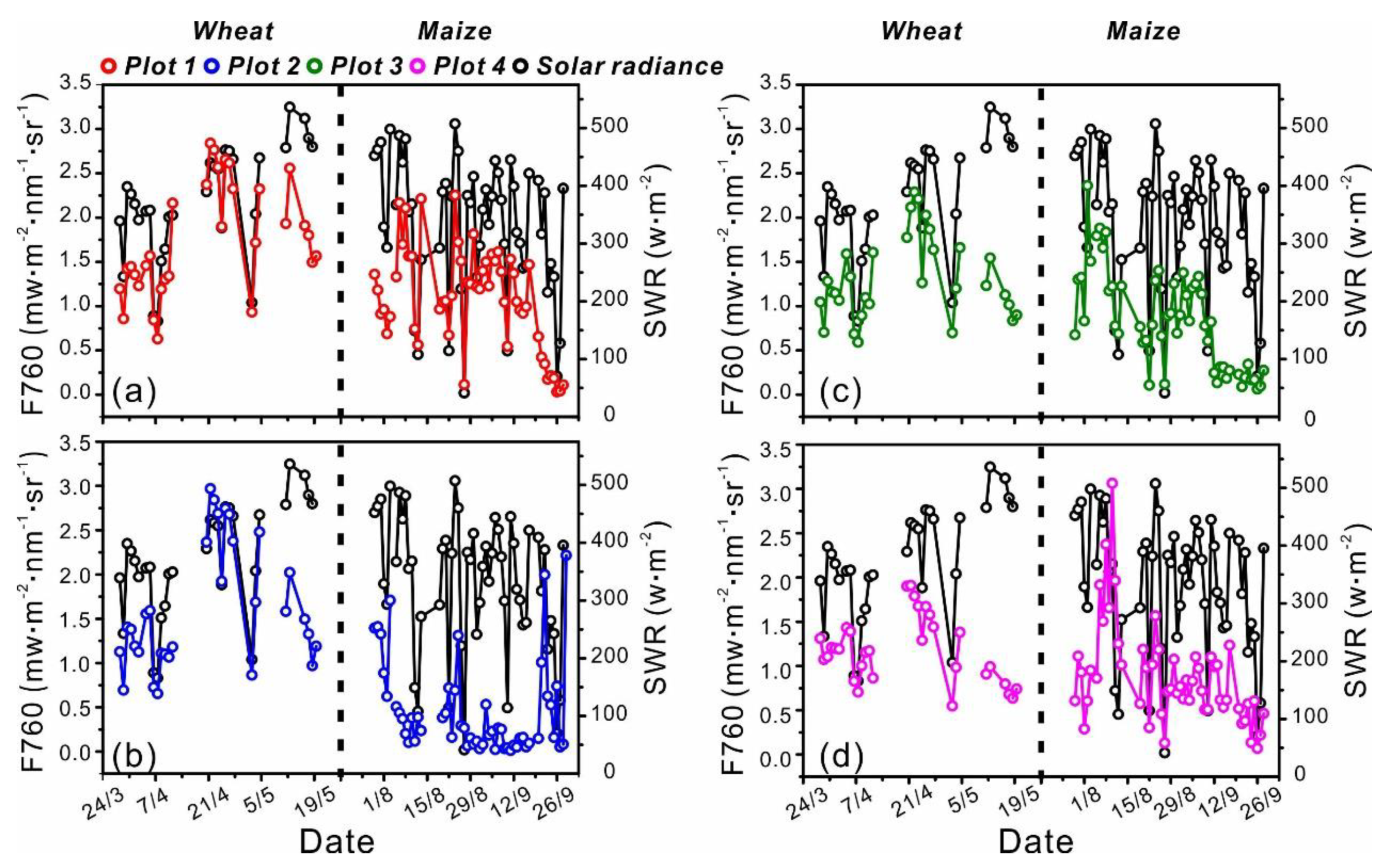
3.1. Seasonal Patterns of SIF

According to the seasonal patterns shown in Figure 3, the F760 of wheat and maize showed large day-to-day variations, which agreed well with the daily variation of SWR, except plot 2 for maize. This indicated that SWR might be a main driver for the seasonal patterns of F760, which was consistent with the findings in a temperate deciduous forest [9]. We also found that F760 in the late period (particularly after May for wheat and after September for maize) could not reach the same magnitude as the early growth stage, even as the concurrent SWR was at similar or higher levels (Figure 3). This result implied that seasonal patterns of F760 might also be related to plant phenological stages. Based on the observations of wheat in Figure 3 (can also be seen in Figure S1), gradient values of F760 were also observed after 22 April 2017, during which, wheat was suffering from gradient irrigation treatments (Figure 2b). These gradient F760 over the four plots showed similar daily variations but with a decreasing trend in the order plot 1 > plot 2 > plot 3 > plot 4 (Figure 3 and Figure S1), corresponding to the decreasing order of irrigation amounts in the four plots (Figure 2b). The consistent decreasing trend of F760 with gradient irrigation treatments suggested that water stress may yield lower F760 values and thus suggested that soil moisture was another factor affecting the emission of SIF. It was expected that the seasonal patterns of maize F760 in the four plots should show little differences since rain was applied over the maize during its whole growth season. As expected, F760 in plot 1, plot 3, and plot 4 differed slightly between each other (Figure 3). However, maize F760 in plot 2 showed much lower values than that of the other three plots, particularly in the period between 25 August and 17 September 2017. This abnormal phenomenon may be attributed to the unsuitable spectra collection position that led to a close distance between the bare fiber and the top leaves, which thereby lowered the canopy radiance received by the sensor.

Similar with F760, the seasonal patterns of AF760 and Fy760 also tracked the seasonal pattern of SWR (Figure 4). This means that SWR still played important roles in driving the seasonal patterns of AF760 and Fy760. However, the covariation of SWR with AF760 and Fy760 was not totally consistent: AF760 changed consistently with SWR during the whole periods, while Fy760 showed a similar situation before May for wheat and before middle September for maize, and a reversed situation after that time (Figure 4). This result also drew the conclusion that the role of plant phenological stages was also important for driving the seasonal patterns of AF760 and Fy760, which was similar with that of F760.

Furthermore, compared with F760, AF760 and Fy760 exhibited smaller daily fluctuations during the field campaigns (Figure 4 and Figure S1). These smaller fluctuations resulted from the partial removal of solar radiance impacts through the method of F760/PAR and F760/L685. In addition, the water-stress-induced difference of wheat Fy760 among the four plots could be distinguished from 22 April (the time that gradient irrigations were applied), which was obviously earlier than that of F760 and AF760 (gradients among the four plots were observed after May) (Figure 4 and Figure S1). On the contrary, relative to F760, rain-fed maize AF760 showed a smaller difference among plot 1, plot 3, and plot 4 and Fy760 in these three plots (Figure 4 and Figure S1). AF760 and Fy760 of maize in plot 2 still remained lower than that of the other three plots (Figure 4 and Figure S1).

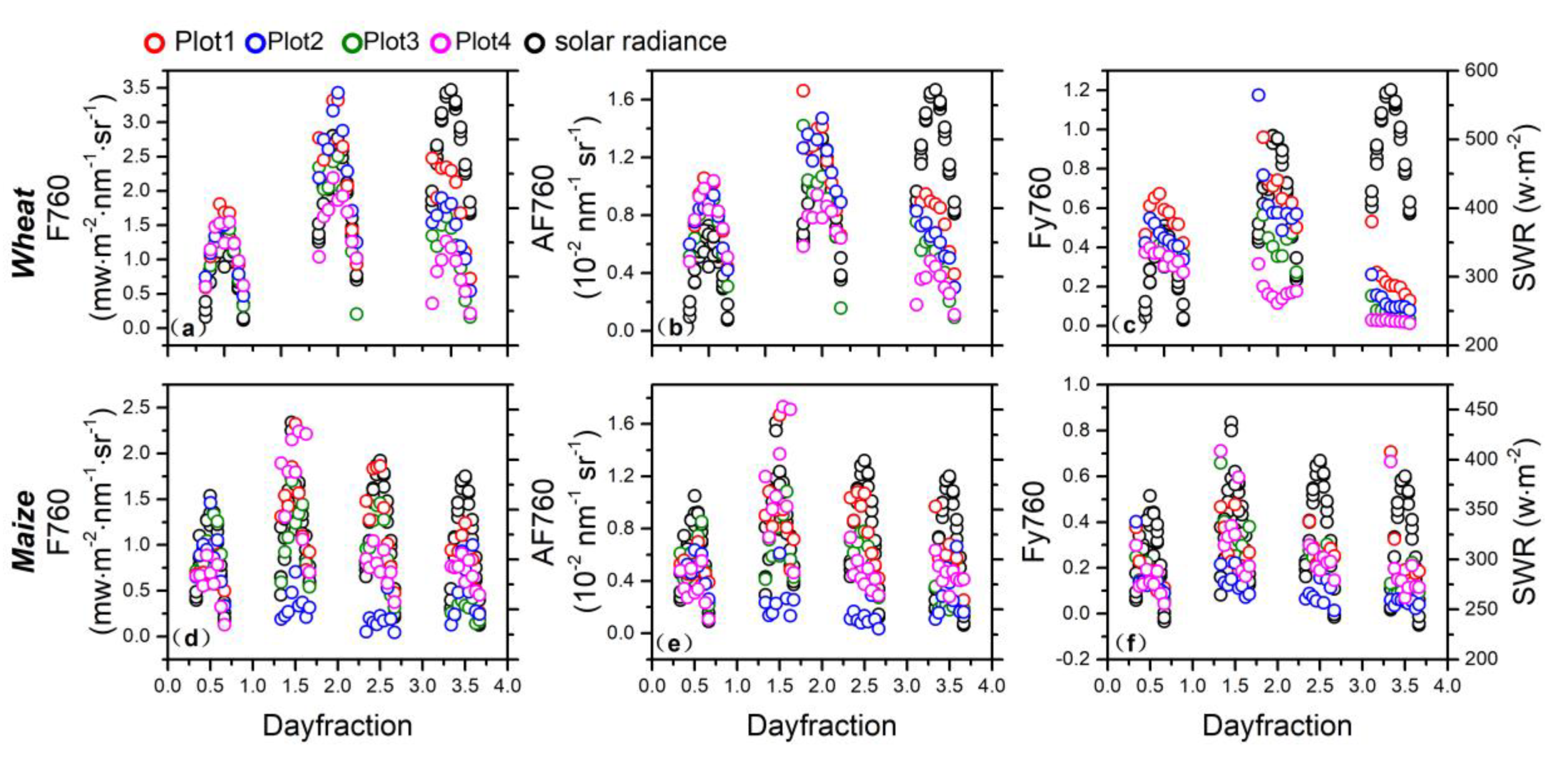
3.2. Diurnal Patterns of SIF

For the diurnal patterns, wheat F760 (one-hour interval) averaged for each of the 15 days showed a typical hump shape with a steady increase in the morning and decline in the afternoon (Figure 5a). Averaged one-hour values of maize F760 across 15 days also showed similar patterns as that of hourly F760 of wheat (Figure 5d). As observed with seasonal patterns, diurnal patterns of F760 similarly followed the diurnal variations of SWR (Figure 5a,d), suggesting that SWR was also a main driver for the diurnal variation of F760. A similar effect of SWR in driving diurnal patterns of AF760 was also found from wheat measurements (Figure 5b). Nevertheless, the effect of SWR was indistinct for diurnal patterns of wheat Fy760 (Figure 5c). Such an indistinct effect of SWR was more prominent for diurnal patterns of maize AF760 and Fy760 (Figure 5e,f).

Furthermore, the magnitude of diurnal F760, AF760, and Fy760 in each plot showed apparent fluctuations with the development of wheat and maize (Figure 5). Part of these fluctuations might have been due to the variation of SWR, such as the first two diurnal patterns (Figure 5). However, plant phenological stages might have also played an important role in driving the fluctuation because these values in the third diurnal patterns of wheat and fourth diurnal pattern of maize were much lower than that of previous patterns, even if homochronous SWR values were higher or approximate compared to SWR of previous patterns (Figure 5).

We also found that the differences of wheat F760 and AF760 between each plot were indistinct in the first diurnal pattern but were distinct in the last two patterns (Figure 5a,b). Furthermore, the difference in wheat Fy760 between each plot were distinct for all three diurnal patterns. The differences of these diurnal SIF patterns showed distinguishable and decreasing hourly values in the order plot 1 > plot 2 > plot 3 > plot 4, particularly in the third 15-day period (12 to 21 May 2017) of wheat (Figure 5a–c). The decreasing order of diurnal SIF (F760, AF760, and Fy760) was consistent with the irrigation gradient applied over the four plots, thus suggesting that water stress also affected the diurnal SIF patterns. Without the influence of water stress, the magnitude of peak values of maize SIF declined from the second diurnal pattern as the season progressed. This continuous decrease of peak values agrees well with the progress of the phenological stages. On one hand, this further confirmed that plant phenological stages are another important factor driving the diurnal patterns of SIF. On the other hand, this revealed that peak SIF values at noon might provide meaningful information for SIF diurnal patterns.

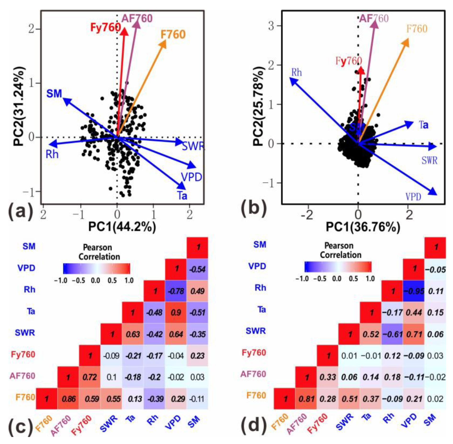
3.3. The Impacts of Growth and Environmental Parameters on Seasonal SIF

To elucidate the relationship of seasonal SIF patterns (including F760, AF760, and Fy760) with environmental and growth parameters, we applied principal component analysis (PCA) based on the daily measurements of wheat and maize, respectively (Figure 6). Two dominating factors were identified using PCA as PC1 and PC2, which were responsible for 37.07% and 31.68% for wheat and 34.12% and 26.94% for maize, respectively, of the variance in all parameter distributions (Figure 6).

As described in Figure 6a,b, non-right angles were found between F760 and all environmental parameters both for wheat and maize, showing that all these parameters played important roles in controlling seasonal patterns of F760. Their impacts on wheat seasonal F760 was in the order of Rh, SWR, VPD, SM, and Ta (r values: −0.55, 0.43, 0.35, 0.08, and 0.06, respectively), while their impacts on maize F760 was in the order of Ta, SWR, SM, Rh, and VPD (r values: 0.43, 0.14, −0.09, 0.03, and 0, respectively). Moreover, the correlation between Rh and wheat F760 and the correlation between Ta and maize F760 were significant (p < 0.05), indicating that Rh and Ta were vitally important environmental drivers for the seasonal variation of F760 from wheat and maize, respectively. Similarly, PCA outputs showed that all growth parameters (LAI, Chl, MTA, and RWC) are also important for driving the seasonal patterns of F760 due to their non-right angles with F760. However, LAI and MTA were believed to be more important drivers than other growth parameters for seasonal wheat F760 because of their significant correlations (0.63 and −0.63, respectively; p < 0.05). Unlike wheat, maize F760 only significantly and negatively correlated with MTA (−0.53, p < 0.05), which means that MTA was vitally important for the seasonal pattern of maize F760.

The effects of these environmental and growth parameters on AF760 and Fy760 were different from F760. Specifically, the impacts of SWR on AF760 and Fy760 became weaker according to the observation of their nearly right angles in the PCA coordinates (Figure 6a). Such weaker impacts were further confirmed by the lower correlations of SWR with AF760 and Fy760 (−0.2 and 0.01, Figure 6c). In addition, both VPD and Rh also showed weaker correlations with AF760 and Fy760 (VPD: −0.28 and −0.05; Rh: −0.06 and −0.05, respectively; Figure 6c), possibly due to the covariation of VPD and Rh with SWR (r values: 0.99 and −0.76, p < 0.05). Although Ta was also covariant with SWR (r value: 0.78, p < 0.01), it only showed a weaker correlation with Fy760 (0.11, Figure 6c). On the contrary, SM showed smaller acute angles with AF760 and Fy760, which indicated that SM was more important for seasonal AF760 and Fy760 relative to F760 (Figure 6a). Wheat AF760 and Fy760 were also affected by all growth parameters based on the PCA results (Figure 6a). Among these growth parameters, both LAI and RWC showed significantly correlations with AF760 (r values: 0.69 and 0.60, p < 0.01), indicating their most important roles in driving seasonal patterns of AF760. For maize seasonal patterns of AF760, the effects of all environmental parameters were insignificant except for Rh, which showed a significant relationship with AF760 (r value: 0.45, p < 0.05, Figure 6b). Similarly, in addition to SM, other environmental parameters, particularly Ta and SWR, were important for the seasonal pattern of Fy760 (Figure 6b,d). Obviously, growth parameters, such as LAI and Chl, were vitally important for the seasonal pattern of Fy760 (r values: 0.66 and 0.75, p < 0.05, Figure 6d). RWC and MTA were more important growth parameters than others in driving the seasonal patterns of AF760 since they showed higher correlations with AF760 than other growth parameters (Figure 6d).

3.4. The Impacts of Growth and Environmental Parameters on Diurnal SIF

To assess the diurnal SIF patterns using PCA, we only analyzed the relationship between hourly SIF and environmental parameters because growth parameters (e.g., LAI, Chl, or RWC) in a day could be considered as constant. Results of PCA showed that SWR was the most important environmental driver for the diurnal variation of F760, both in wheat and maize (r values: 0.55 and 0.51, p < 0.01, Figure 7). Other environmental parameters showed secondary impacts on diurnal F760 with the order of Rh, VPD, Ta, and SM for wheat (r values: 0.39, 0.29, 0.13, and 0.11, respectively) and the order of Ta, VPD, Rh, and SM for maize (r values: 0.37, 0.21, −0.09, and 0.02, respectively; Figure 7). By normalizing F760 with SWR and L685, the impacts of SWR on AF760 and Fy760 distinctly became weaker both for wheat and maize (r values: 0.1 and 0.09 for wheat, 0.06 and 0.01 for maize, respectively; Figure 7). The impacts of VPD and Rh on the variation of AF760 and Fy760 in wheat were also decreased, as well as the impact of VPD and Ta on maize AF760 and Fy760 (Figure 7). Nevertheless, the impacts of Ta on wheat AF760 and Fy760 were larger relative to F760, and similarly with the increased effect of Rh on maize AF760 and Fy760 (Figure 7). Furthermore, for wheat, the effect of SM on Fy760 became larger but vanished on AF760.

From the diurnal patterns of SIF, we found that SIF at noon time could further reflect the variation of diurnal SIF with the development of phenological stages (Figure 5). Thus, relationships between SIF at noon time and growth parameters were further analyzed through analyzing the Pearson correlation. Based on the analysis over wheat measurements, we found that F760, AF760, and Fy760 at noon time were mainly affected by LAI (r values: 0.56, 0.53, and 0.54, Figure 8a). The considerable impact of Chl on F760 and AF760, but negligible impact of Chl on Fy760, were observed (r values: 0.51, 0.5, and 0.13, respectively; Figure 8a). The impact of RWC was significant on AF760 and Fy760 but insignificant on F760 (r values: 0.64, 0.9, and 0.08, respectively; Figure 8a). However, based on maize measurements, we found that most growth parameters played negligible roles for driving diurnal variation of F760, AF760, and Fy760. Only Chl showed a significant correlation with Fy760 (r value: 0.27, p < 0.01; Figure 8b), and therefore played an important role in driving the diurnal pattern of Fy760.

4. Discussion

In this study, the impacts of growth and environmental parameters on SIF (F760, AF760, and Fy760) were systematically analyzed based on continuous ground measurements over wheat and maize. Different time scales, i.e., seasonal and diurnal scales, were also considered in our analysis. The above results suggested that both seasonal and diurnal SIF patterns were affected by growth and environmental parameters. In order to better understand those parameters’ impacts on SIF emissions at seasonal and diurnal scales, their impacts on F760 and AF760/Fy760 were further considered separately. The influence of water stress and phenology on the variations of F760, AF760, and Fy760 were also further investigated in this section.

4.1. Further Understanding about the Relationship of F760 with Growth and Environmental Parameters

Based on the results mentioned in the previous sections, we know that seasonal and diurnal F760 patterns were completely different (Figure 3 and Figure 5). However, both of them were mainly driven by the variation of SWR. We also noted that the impact of SWR on seasonal F760 was less important than other environmental parameter (i.e., Rh for wheat and Ta for maize) (Figure 6). This may be because measurements for analyzing seasonal F760 were only from part of the whole growth periods since SWR was believed to be a more important environmental parameter in driving the seasonal pattern of F760 in whole-field campaigns (Figure S2).

Ta, Rh, and VPD were three other important environmental parameters that could affect F760 variations at seasonal and diurnal scales. This could be explained by the fact that Ta, Rh, and VPD could affect air aridity, and therefore alter transpiration by regulating the water demand of air from vegetation and ultimately affect photosynthesis [45]. However, we should also note that relationships of F760 with Ta, Rh, and VPD were different between wheat and maize (Figure 6 and Figure 7). That is to say, the impact of these parameters on seasonal F760 variation was varied with different plant functional types. For diurnal scales, both of the relationships of F760 with wheat and maize were significant (Figure 7), which means that air aridity was a key factor in controlling diurnal F760 variation. Although SM-induced water stress lowered SIF magnitudes, both at seasonal and diurnal scales (Figure 3a and Figure 5a), SM did not show a considerable relationship with F760 (r values: 0.08 and 0.11 for wheat, −0.09 and 0.02 for maize, at seasonal and diurnal scales, respectively; Figure 6c,d and Figure 7c,d)

The seasonal and diurnal patterns of F760 were also affected by growth parameters, which included LAI, Chl, MTA, and RWC. Based on wheat measurements, both LAI, Chl, and MTA played crucial roles in regulating F760, not only at the seasonal scale, but also at the diurnal scale (Figure 6 and Figure 7). This was because LAI, Chl, and MTA were related to the canopy structure that determined light capture by the canopy. However, these three parameters, particularly LAI and Chl, did not show significant impacts on maize SIF at both the seasonal and diurnal scales. This large deviation from the results of wheat may be explained by the more complicated canopy structure of maize than that of wheat. Additionally, the short observation distance between the fiber and canopy may be another explanation for such results, since the short distance results in a small view area of the fiber, and therefore only a partial signal of canopy can be received by the sensor. RWC was also important for F760 variation at seasonal and diurnal scales, which was demonstrated by the relatively high correlation between RWC and SIF observed in maize (r values: 0.42 and 0.21, at seasonal and diurnal scales, respectively; Figure 6d and Figure 8b). The importance of RWC for SIF variation is attributed to the close relationship between RWC and photosynthesis: RWC directly indicates the plant water content, which influences the photosynthesis rate and light capture by leaf wilting and leaf angle adjustments [46]. The leaf angle adjustments by the variation of RWC was supported by high correlation between RWC and MTA based on the measurements of maize (−0.53 for seasonal scale, −0.58 for diurnal scale, Figure 6d and Figure 8b).

As mentioned above, it can be concluded that F760 was mainly driven by SWR for the environmental parameters and LAI, Chl, MTA, and RWC for the growth parameters, while being less driven by Ta, VPD, Rh, and SM. A similar result has been reported by Verrelst et al. with the simulated data of the Soil-Canopy Observation of Photosynthesis and Energy (SCOPE) balance model [47]. The contribution of each parameter to SIF is further affected by plant functional types, as revealed by the data from wheat and maize in our study. This has been partly explained by Rossini et al., who showed that LAI is not the main factor for driving F760 differences between species from different plant functional types [31]. In fact, biochemical properties may play an important role in driving F760 differences across plant functional types. The role of biochemical properties (e.g., fraction of functional reaction centers, maximum carboxylation capacity, and rate constant of sustained thermal dissipation) was more remarkable for SIF yield [47], which will be further discussed in Section 4.2 and Section 4.3.

4.2. Further Understanding about the Relationship of AF760 and Fy760 with Growth and Environmental Parameters

Compared with F760, the dependences of AF760 and Fy760 on SWR were much smaller, which was deduced from their weaker relationships, especially for both seasonal and diurnal patterns of wheat and the diurnal pattern of maize (Figure 6 and Figure 7). This was because of the removal of the SWR influence by means of F760/SWR and F760/L685. With less dependence of AF760 and Fy760 on SWR, both AF760 and Fy760 generally showed weaker relationships with VPD, Ta, and Rh relative to F760. This result is attributed to the fact that partial information of AF760 and Fy760 with Ta, Rh, and VPD were simultaneously removed by F760/SWR and F760/L685, since Ta, Rh, and VPD were covariant with SWR. When the impacts of air parameters (Ta, Rh, and VPD) on AF760 and Fy760 were partially removed, the influence of SM both on AF760 and Fy760 became larger, especially for wheat measurements, most of which may have suffered from water stress.

After removing the influence of SWR by using F760/SWR, it was expected that AF760 at seasonal and diurnal scales would show an enhanced relationship with growth parameters. However, this assumption was only established for wheat LAI and RWC at the seasonal scale, which showed an enhanced impact on AF760 (Figure 6). Other growth parameters (e.g., Chl and MTA) did not show obviously enhanced effects in affecting AF760, both at seasonal and diurnal scales for wheat and for maize (Figure 6 and Figure 8). This means that the impacts of LAI and RWC for AF760 at different time scales were more pronounced. Fy760 was more closely related to SIF yield than AF760 since it removed the partial influence of SWR on one hand and eliminates the canopy structure influence on the other hand [39]. Therefore, in the wheat plots, the influence of LAI, Chl, and MTA showed a reduced relationship with Fy760 compared with AF760. In maize plots, similar results were also found for the seasonal relationship of MTA and RWC in relating with Fy760. LAI and Chl in maize plots did not show consistent results, which might be attributed to the complicated canopy structure and close distance between the fiber and canopy.

In our study, the greater influence of structural variables (e.g., LAI) on AF760 than F760 was also observed, which was not consistent with the findings by Verrelst et al., who reported a lower sensitivity of SIF yield to structural variables. This was probably due to the SIF yield in Verrelst et al. being calculated by using hemispherically integrated flux, which is much less influenced by these structural variables than the fluorescence in a single observation in our study.

4.3. Insights from the Impacts of Water Stress and Phenological Stages

In order to further understand the influence of water stress, it should be considered that SIF at 760 nm was contributed by the combination of two photosystems (photosystems I and II) [1], which could be greatly affected by water stress. Specifically, water stress is known as a limiting environmental parameter that results in the down-regulation of photosynthesis through stomatal closure [48,49,50] or metabolic impairment [51,52]. Down-regulation of photosynthesis generally lowers the absorption of solar radiation, which thereby causes the decline of SIF emissions. This result was also confirmed by our wheat observations, which showed decreasing SIF (F760, AF760, and Fy760) values at seasonal and diurnal scales accompanied with intensifying water stress (Figure 3, Figure 4 and Figure 5a–c). Furthermore, the down-regulation of photosynthesis finally leads to the inhibition of plant growth [53]. This was also demonstrated in our study by the decreasing LAI values with the increasing of water stress over the four plots of wheat (Figure S3). This decreased LAI values under water stress would further lower the absorption of solar radiation due to the lower solar capture, and further lowered the SIF emission (Figure S4).

Additionally, water stress is often accompanied by high values of Ta (optimal Ta for plants normal growth is about 10–35 °C) and VPD (in general greater than 2 kPa, meaning low humidity), which could also affect the stomatal conductance of leaves and further decrease photosynthetic capacity [54,55]. In our study, high values of Ta and VPD were not observed at seasonal and diurnal scales; however, their impacts on SIF radiance cannot be ignored, particularly for Ta in wheat plots, some of which were suffering from water stress. This conclusion can be further confirmed by the relative high correlation between Ta and AF760 at the wheat seasonal scale (Figure 6c). This was because water stress could cause the increase of intercellular CO₂ level and the decrease of stomatal conductance, which would greatly sharpen the response of photosynthesis to the variation of temperature [52].

Phenological stages were also found to be an important factor in driving the variation of SIF, both on seasonal and diurnal scales. This was because phenological stages can determine the timing of plant development (e.g., LAI) and behavioral phases of organisms, such as bud burst, flowering, leaf coloration, and senescence [56,57,58]. That is to say, the impact of phenological stages on SIF may be integrated from the impact of LAI or leaf coloration (i.e., leaf greenness). Their synergistic effects may explain the drop of SIF after May for wheat and after September for maize, although concurrent SWRs were similar to before. (Figure 3 and Figure 5). Their mixed influence on SIF variation might bring much trouble in exploring the detailed relationships between phenological stages and SIF. Moreover, phenological phases of plants are mainly driven by air temperature, photoperiod length, and are less impacted by water availability, nutrients, and soil properties [56,57,58,59]. This makes it more complicated for understanding the impact of phenology on SIF emissions.

5. Conclusions

In this study, field campaigns were conducted over wheat and maize and continuous ground measurements of SIF (including F760, AF760, and Fy760) were collected based on an automated spectroscopy system. Growth parameters (including LAI, Chl, MTA, and RWC) and environmental parameters (including SWR, Ta, VPD, and SM) were also measured during the field campaigns. Based on this data set, the seasonal and diurnal patterns of SIF were described. Most importantly, we systematically assessed the impacts of both growth and environmental parameters on SIF variation at different time scales. Our results suggested that SIF was affected by both growth and environmental parameters.

Specifically, F760 was mainly driven by SWR for environmental parameters and LAI, Chl, MTA, and RWC for growth parameters, while being less driven by Ta, VPD, and Rh due to their covariation with SWR. SM also affected seasonal and diurnal patterns of F760 when SM was at a deficit. With the removal of influence from SWR, both AF760 and Fy760 were likely to be less dependent on Ta, Rh, and VPD, while an enhanced relationship of AF760 and Fy760 with SM was particularly observed under water stress. Wheat AF760 was more related to LAI and RWC than F760, as expected, while maize AF760 did not show an enhanced relationship with all growth parameters compared with F760, mostly due to its complicated canopy structure. Compared with AF760, the relationship of Fy760 with canopy structure parameters were further reduced, except for maize measurements. SM-induced water stress could lower the SIF radiance not only by limiting photosynthesis but also by inhibiting plant growth (e.g., LAI in our study); thus, much more attention should be paid when the relationship of SIF with each parameter is interpreted. The impacts of phenological stages on SIF were always present over both seasonal and diurnal scales. This suggests that SIF might be used as a potential indicator for exploring the phenological variation with the global climate change.

References

1. Porcar-Castell, A.; Tyystjärvi, E.; Atherton, J.; van der Tol, C.; Flexas, J.; Pfündel, E.E.; Moreno, J.; Frankenberg, C.; Berry, J.A. Linking chlorophyll a fluorescence to photosynthesis for remote sensing applications: Mechanisms and challenges. J. Exp. Bot. 2014, 65, 4065–4095. [Google Scholar] [CrossRef] [PubMed]
2. Sun, Y.; Frankenberg, C.; Wood, J.D.; Schimel, D.S.; Jung, M.; Guanter, L.; Drewry, D.T.; Verma, M.; Porcarcastell, A.; Griffis, T.J. OCO-2 advances photosynthesis observation from space via solar-induced chlorophyll fluorescence. Science 2017, 358, eaam5747. [Google Scholar] [CrossRef] [PubMed] [Green Version]
3. Meroni, M.; Busetto, L.; Colombo, R.; Guanter, L.; Moreno, J.; Verhoef, W. Performance of spectral fitting methods for vegetation fluorescence quantification. Remote Sens. Environ. 2010, 114, 363–374. [Google Scholar] [CrossRef]
4. Rossini, M.; Nedbal, L.; Guanter, L.; Ač, A.; Alonso, L.; Burkart, A.; Cogliati, S.; Colombo, R.; Damm, A.; Drusch, M. Red and far red Sun-induced chlorophyll fluorescence as a measure of plant photosynthesis. Geophys. Res. Lett. 2015, 42, 1632–1639. [Google Scholar] [CrossRef]
5. Meroni, M.; Rossini, M.; Guanter, L.; Alonso, L.; Rascher, U.; Colombo, R.; Moreno, J. Remote sensing of solar-induced chlorophyll fluorescence: Review of methods and applications. Remote Sens. Environ. 2009, 113, 2037–2051. [Google Scholar] [CrossRef]
6. Liu, L.; Zhang, Y.; Wang, J.; Zhao, C. Detecting solar-induced chlorophyll fluorescence from field radiance spectra based on the Fraunhofer line principle. IEEE Trans. Geosci. Remote Sens. 2005, 43, 827–832. [Google Scholar]
7. Pérez-Priego, O.; Zarco-Tejada, P.J.; Miller, J.R.; Sepulcre-Cantó, G.; Fereres, E. Detection of water stress in orchard trees with a high-resolution spectrometer through chlorophyll fluorescence in-filling of the O/sub 2/-A band. IEEE Trans. Geosci. Remote Sens. 2005, 43, 2860–2869. [Google Scholar] [CrossRef]
8. Daumard, F.; Goulas, Y.; Champagne, S.; Fournier, A.; Ounis, A.; Olioso, A.; Moya, I. Continuous monitoring of canopy level sun-induced chlorophyll fluorescence during the growth of a sorghum field. IEEE Trans. Geosci. Remote Sens. 2012, 50, 4292–4300. [Google Scholar] [CrossRef]
9. Yang, X.; Tang, J.; Mustard, J.F.; Lee, J.E.; Rossini, M.; Joiner, J.; Munger, J.W.; Kornfeld, A.; Richardson, A.D. Solar-induced chlorophyll fluorescence that correlates with canopy photosynthesis on diurnal and seasonal scales in a temperate deciduous forest. Geophys. Res. Lett. 2015, 42, 2977–2987. [Google Scholar] [CrossRef]
10. Zarco-Tejada, P.J.; Berni, J.A.; Suárez, L.; Sepulcre-Cantó, G.; Morales, F.; Miller, J. Imaging chlorophyll fluorescence with an airborne narrow-band multispectral camera for vegetation stress detection. Remote Sens. Environ. 2009, 113, 1262–1275. [Google Scholar] [CrossRef]
11. Zarco-Tejada, P.J.; Morales, A.; Testi, L.; Villalobos, F.J. Spatio-temporal patterns of chlorophyll fluorescence and physiological and structural indices acquired from hyperspectral imagery as compared with carbon fluxes measured with eddy covariance. Remote Sens. Environ. 2013, 133, 102–115. [Google Scholar] [CrossRef]
12. Lee, J.-E.; Frankenberg, C.; van der Tol, C.; Berry, J.A.; Guanter, L.; Boyce, C.K.; Fisher, J.B.; Morrow, E.; Worden, J.R.; Asefi, S. Forest productivity and water stress in Amazonia: Observations from GOSAT chlorophyll fluorescence. Proc. R. Soc. B Biol. Sci. 2013, 280, 20130171. [Google Scholar] [CrossRef]
13. Yoshida, Y.; Joiner, J.; Tucker, C.; Berry, J.; Lee, J.-E.; Walker, G.; Reichle, R.; Koster, R.; Lyapustin, A.; Wang, Y. The 2010 Russian drought impact on satellite measurements of solar-induced chlorophyll fluorescence: Insights from modeling and comparisons with parameters derived from satellite reflectances. Remote Sens. Environ. 2015, 166, 163–177. [Google Scholar] [CrossRef]
14. Sun, Y.; Fu, R.; Dickinson, R.; Joiner, J.; Frankenberg, C.; Gu, L.; Xia, Y.; Fernando, N. Drought onset mechanisms revealed by satellite solar-induced chlorophyll fluorescence: Insights from two contrasting extreme events. J. Geophys. Res. Biogeosci. 2016, 120, 2427–2440. [Google Scholar] [CrossRef]
15. Wang, S.; Huang, C.; Zhang, L.; Lin, Y.; Cen, Y.; Wu, T. Monitoring and Assessing the 2012 Drought in the Great Plains: Analyzing Satellite-Retrieved Solar-Induced Chlorophyll Fluorescence, Drought Indices, and Gross Primary Production. Remote Sens. 2016, 8, 61. [Google Scholar] [CrossRef]
16. Liu, L.; Cheng, Z. Detection of Vegetation Light-Use Efficiency Based on Solar-Induced Chlorophyll Fluorescence Separated From Canopy Radiance Spectrum. IEEE J. Sel. Top. Appl. Earth Obs. Remote Sens. 2010, 3, 306–312. [Google Scholar] [CrossRef]
17. Zhang, Y.; Guanter, L.; Berry, J.A.; Tol, C.V.D.; Joiner, J. Can we retrieve vegetation photosynthetic capacity paramter from solar-induced fluorescence? In Proceedings of the Geoscience and Remote Sensing Symposium, Beijing, China, 10–15 July 2016; pp. 1711–1713. [Google Scholar]
18. Joiner, J.; Yoshida, Y.; Vasilkov, A.P.; Yoshida, Y.; Corp, L.A.; Middleton, E.M. First observations of global and seasonal terrestrial chlorophyll fluorescence from space. Biogeosci. Discuss. 2011, 8, 637–651. [Google Scholar] [CrossRef] [Green Version]
19. Beer, C.; Reichstein, M.; Tomelleri, E.; Ciais, P.; Jung, M.; Carvalhais, N.; Rödenbeck, C.; Arain, M.A.; Baldocchi, D.; Bonan, G.B. Terrestrial Gross Carbon Dioxide Uptake: Global Distribution and Covariation with Climate. Science 2010, 329, 834–838. [Google Scholar] [CrossRef] [Green Version]
20. Peters, W.; Jacobson, A.R.; Sweeney, C.; Andrews, A.E.; Conway, T.J.; Masarie, K.; Miller, J.B.; Bruhwiler, L.M.P.; Gabrielle, P.; Hirsch, A.I. An atmospheric perspective on North American carbon dioxide exchange: CarbonTracker. Proc. Natl. Acad. Sci. USA 2007, 104, 18925–18930. [Google Scholar] [CrossRef] [Green Version]
21. Guanter, L.; Frankenberg, C.; Dudhia, A.; Lewis, P.E.; Gómez-Dans, J.; Kuze, A.; Suto, H.; Grainger, R.G. Retrieval and global assessment of terrestrial chlorophyll fluorescence from GOSAT space measurements. Remote Sens. Environ. 2012, 121, 236–251. [Google Scholar] [CrossRef]
22. Guanter, L.; Zhang, Y.; Jung, M.; Joiner, J.; Voigt, M.; Berry, J.A.; Frankenberg, C.; Huete, A.R.; Zarcotejada, P.; Lee, J.E. Global and time-resolved monitoring of crop photosynthesis with chlorophyll fluorescence. Proc. Natl. Acad. Sci. USA 2014, 111, 1327–1333. [Google Scholar] [CrossRef]
23. Frankenberg, C.; O’Dell, C.; Berry, J.; Guanter, L.; Joiner, J.; Köhler, P.; Pollock, R.; Taylor, T.E. Prospects for chlorophyll fluorescence remote sensing from the Orbiting Carbon Observatory-2. Remote Sens. Environ. 2014, 147, 1–12. [Google Scholar] [CrossRef] [Green Version]
24. Campbell, P.K.; Middleton, E.M.; Corp, L.A.; Kim, M.S. Contribution of chlorophyll fluorescence to the apparent vegetation reflectance. Sci. Total Environ. 2008, 404, 433. [Google Scholar] [CrossRef]
25. Cogliati, S.; Rossini, M.; Julitta, T.; Meroni, M.; Schickling, A.; Burkart, A.; Pinto, F.; Rascher, U.; Colombo, R. Continuous and long-term measurements of reflectance and sun-induced chlorophyll fluorescence by using novel automated field spectroscopy systems. Remote Sens. Environ. 2015, 164, 270–281. [Google Scholar] [CrossRef]
26. Verma, M.; Schimel, D.; Evans, B.; Frankenberg, C.; Beringer, J.; Drewry, D.T.; Magney, T.; Marang, I.; Hutley, L.; Moore, C. Effect of environmental conditions on the relationship between solar-induced fluorescence and gross primary productivity at an OzFlux grassland site. J. Geophys. Res. Biogeosci. 2017, 122, 716–733. [Google Scholar] [CrossRef]
27. Damm, A.; Guanter, L.; Paul-Limoges, E.; Tol, C.V.D.; Hueni, A.; Buchmann, N.; Eugster, W.; Ammann, C.; Schaepman, M.E. Far-red sun-induced chlorophyll fluorescence shows ecosystem-specific relationships to gross primary production: An assessment based on observational and modeling approaches. Remote Sens. Environ. 2015, 166, 91–105. [Google Scholar] [CrossRef]
28. Hernández-Clemente, R.; North, P.R.J.; Hornero, A.; Zarco-Tejada, P.J. Assessing the effects of forest health on sun-induced chlorophyll fluorescence using the FluorFLIGHT 3-D radiative transfer model to account for forest structure. Remote Sens. Environ. 2017, 193, 165–179. [Google Scholar] [CrossRef] [Green Version]
29. Liu, L.; Liu, X.; Guan, L. Uncertainties in linking solar-induced chlorophyll fluorescence to plant photosynthetic activities. In Proceedings of the Geoscience and Remote Sensing Symposium, Beijing, China, 10–15 July 2016; pp. 4414–4417. [Google Scholar]
30. Goulas, Y.; Fournier, A.; Daumard, F.; Champagne, S.; Ounis, A.; Marloie, O.; Moya, I. Gross Primary Production of a Wheat Canopy Relates Stronger to Far Red Than to Red Solar-Induced Chlorophyll Fluorescence. Remote Sens. 2017, 9, 97. [Google Scholar] [CrossRef]
31. Rossini, M.; Meroni, M.; Celesti, M.; Cogliati, S.; Julitta, T.; Panigada, C.; Rascher, U.; Tol, C.V.D.; Colombo, R. Analysis of Red and Far-Red Sun-Induced Chlorophyll Fluorescence and Their Ratio in Different Canopies Based on Observed and Modeled Data. Remote Sens. 2016, 8, 412. [Google Scholar] [CrossRef]
32. Liu, L.; Yang, X.; Zhou, H.; Liu, S.; Zhou, L.; Li, X.; Yang, J.; Han, X.; Wu, J. Evaluating the utility of solar-induced chlorophyll fluorescence for drought monitoring by comparison with NDVI derived from wheat canopy. Sci. Total Environ. 2018, 625, 1208–1217. [Google Scholar] [CrossRef]
33. Liu, L.; Yang, X.; Zhou, H.; Liu, S.; Zhou, L.; Li, X.; Yang, J.; Wu, J. Relationship of root zone soil moisture with solar-induced chlorophyll fluorescence and vegetation indices in winter wheat: A comparative study based on continuous ground-measurements. Ecol. Indic. 2018, 90, 9–17. [Google Scholar] [CrossRef]
34. Liu, C.; Zhang, X.; Zhang, Y. Determination of daily evaporation and evapotranspiration of winter wheat and maize by large-scale weighing lysimeter and micro-lysimeter. Agric. For. Meteorol. 2002, 111, 109–120. [Google Scholar] [CrossRef]
35. Sun, H.Y.; Liu, C.M.; Zhang, X.Y.; Shen, Y.J.; Zhang, Y.Q. Effects of irrigation on water balance, yield and WUE of winter wheat in the North China Plain. Agric. Water Manag. 2006, 85, 211–218. [Google Scholar] [CrossRef]
36. Xiao, J.F.; Liu, Z.D.; Chen, Y.M. Study on the Water Requirement and Water Requirement Regulation of Maize in China. J. Maize Sci. 2008, 16, 21–25. (In Chinese) [Google Scholar]
37. Peñuelas, J.; Filella, I.; Biel, C.; Serrano, L.; Save, R. The reflectance at the 950–970 nm region as an indicator of plant water status. Int. J. Remote Sens. 1993, 14, 1887–1905. [Google Scholar] [CrossRef]
38. Köksal, E.S. Hyperspectral reflectance data processing through cluster and principal component analysis for estimating irrigation and yield related indicators. Agric. Water Manag. 2011, 98, 1317–1328. [Google Scholar] [CrossRef]
39. Daumard, F.; Champagne, S.; Fournier, A.; Goulas, Y.; Ounis, A.; Hanocq, J.-F.; Moya, I. A field platform for continuous measurement of canopy fluorescence. IEEE Trans. Geosci. Remote Sens. 2010, 48, 3358–3368. [Google Scholar] [CrossRef]
40. Legendre, P.; Legendre, L.F.J. Numerical Ecology; Elsevier: Amsterdam, The Netherlands, 2012; Volume 24. [Google Scholar]
41. Borcard, D.; Gillet, F.; Legendre, P.X. Numerical Ecology with R; Springer: Berlin/Heidelberg, Germany, 2018. [Google Scholar]
42. Sleighter, R.L.; Liu, Z.; Xue, J.; Hatcher, P.G. Multivariate statistical approaches for the characterization of dissolved organic matter analyzed by ultrahigh resolution mass spectrometry. Environ. Sci. Technol. 2010, 44, 7576–7582. [Google Scholar] [CrossRef]
43. Xue, J.; Lee, C.; Wakeham, S.G.; Armstrong, R.A. Using principal components analysis (PCA) with cluster analysis to study the organic geochemistry of sinking particles in the ocean. Org. Geochem. 2011, 42, 356–367. [Google Scholar] [CrossRef]
44. Oksanen, J.; Blanchet, F.G.; Friendly, M.; Kindt, R.; Legendre, P.; McGlinn, D.; Minchin, P.R.; O’Hara, R.B.; Simpson, G.L.; Solymos, P.; et al. Community Ecology Package. Version 2.5-5. 2019. Available online: https://mirrors.tuna.tsinghua.edu.cn/CRAN/ (accessed on 23 August 2019).
45. Ding, J.; Yang, T.; Zhao, Y.; Liu, D.; Wang, X.; Yao, Y.; Peng, S.; Wang, T.; Piao, S. Increasingly important role of atmospheric aridity on Tibetan alpine grasslands. Geophys. Res. Lett. 2018, 45, 2852–2859. [Google Scholar] [CrossRef]
46. Kramer, P.J.; Boyer, J.S. Water Relations of Plants and Soils; Academic Press: Cambridge, MA, USA, 1995. [Google Scholar]
47. Verrelst, J.; Rivera, J.P.; van der Tol, C.; Magnani, F.; Mohammed, G.; Moreno, J. Global sensitivity analysis of the SCOPE model: What drives simulated canopy-leaving sun-induced fluorescence? Remote Sens. Environ. 2015, 166, 8–21. [Google Scholar] [CrossRef]
48. Flexas, J.; Bota, J.; Galmés, J.; Medrano, H.; Ribas-Carbó, M. Keeping a positive carbon balance under adverse conditions: Responses of photosynthesis and respiration to water stress. Physiol. Plant. 2006, 127, 343–352. [Google Scholar] [CrossRef]
49. Chaves, M.M. Effects of Water Deficits on Carbon Assimilation. J. Exp. Bot. 1991, 42, 1–16. [Google Scholar] [CrossRef]
50. Flexas, J.; Bota, J.; Cifre, J.; Mariano Escalona, J.; Galmés, J.; Gulías, J.; Lefi, E.K.; Teresa Moreno, M.; Ribas-Carbó, M. Understanding down-regulation of photosynthesis under water stress: Future prospects and searching for physiological tools for irrigation management. Ann. Appl. Biol. 2015, 144, 273–283. [Google Scholar] [CrossRef]
51. Boyer, J.S. Photosynthesis at Low Water Potentials. Philos. Trans. R. Soc. Lond. B 1976, 273, 501–512. [Google Scholar] [CrossRef]
52. Lawlor, D.W. Limitation to Photosynthesis in Water-stressed Leaves: Stomata vs. Metabolism and the Role of ATP. Ann. Bot. 2002, 89, 871–885. [Google Scholar] [CrossRef]
53. Chaves, M.M.; Maroco, J.P.; Pereira, J.S. Understanding plant responses to drought-from genes to the whole plant. Funct. Plant Biol. 2003, 30, 239–264. [Google Scholar] [CrossRef]
54. Berry, J.; Bjorkman, O. Photosynthetic response and adaptation to temperature in higher plants. Annu. Rev. Plant Physiol. 1980, 31, 491–543. [Google Scholar] [CrossRef]
55. Chaves, M.M.; Pereira, J.S.; Maroco, J.; Rodrigues, M.L.; Ricardo, C.P.P.; Osório, M.L.; Carvalho, I.; Faria, T.; Pinheiro, C. How plants cope with water stress in the field? Photosynthesis and growth. Ann. Bot. 2002, 89, 907–916. [Google Scholar] [CrossRef]
56. Bondeau, A.; Böttcher, K.; Doktor, D.; Lucht, W.; Schaber, J.; Sitch, S. Responses of Spring Phenology to Climate Change. New Phytol. 2004, 162, 295–309. [Google Scholar]
57. Körner, C.; Basler, D. Phenology under Global Warming. Science 2010, 327, 1461–1462. [Google Scholar] [CrossRef]
58. Morin, X.; Lechowicz, M.J.; Augspurger, C.; O’Keefe, J.; Viner, D.; Chuine, I. Leaf phenology in 22 North American tree species during the 21st century. Glob. Chang. Biol. 2010, 15, 961–975. [Google Scholar] [CrossRef]
59. Menzel, A. Trends in phenological phases in Europe between 1951 and 1996. Int. J. Biometeorol. 2000, 44, 76–81. [Google Scholar] [CrossRef]
Figure 1. The automated spectroscopy system and the field experimental design for wheat and maize. (a) Detailed device configuration for the system. (b,c) Description of the data collection and the location of each data acquisition equipment, respectively.
Remotesensing 11 02002 g001
Figure 2. (a) Precipitation during the period from 15 October 2016 to 29 September 2017, covering the time periods for the field campaigns for wheat and maize. (b) Gradient irrigation treatments applied over the four plots of wheat.
Remotesensing 11 02002 g002
Figure 3. Seasonal patterns of daily F760 from wheat (left of dashed line) and maize (right of dashed line) in the four plots compared with daily solar radiation (SWR). All measurements of wheat were collected from 28 March to 19 May 2017, while the measurements of maize were collected from July 29 to September 29 of 2017.
Remotesensing 11 02002 g003
Figure 4. Seasonal patterns of daily AF760 (first column) and Fy760 (second column) from wheat (left of dashed line in each sub-figure) and maize (right of dashed line in each sub-figure) in the four plots compared with the daily solar radiation (SWR). All measurements of wheat were collected from 28 March to 19 May 2017, while the measurements of maize were collected from July 29 to September 29 of 2017.
Remotesensing 11 02002 g004
Figure 5. Daily patterns of F760 (first column), AF760 (second column), and Fy760 (third column) from wheat (ac) and maize (df) compared with respective solar radiation (SWR). The circles in the figure represent the hourly values that were averaged from the 15-day measurements for wheat and maize. The detailed time periods of wheat were 28/3–11/4, 14/4–28/4 and 12/5–19/5, and the time periods of maize were 29/7–11/8, 12/8–26/8, 27/8–10/9, and 11/9–24/9. The fourth pattern of wheat was only calculated based on the measurements from a week because of the terminal of the field campaign.
Remotesensing 11 02002 g005
Figure 6. Relationships of environmental/growth parameters with F760, AF760, and Fy760 at the seasonal scale. Left column is wheat and right column is maize. (a,b) are PCA results and (c,d) are Pearson correlation results. The relationships between variables in PCA is indicated by vector angle: if the vector angle between two variables is acute, they were positively correlated; else if the angel is obtuse, these two variables were negatively correlated (right angle represents uncorrelated). The smaller the included angle was, the higher the correlation it showed. The significant correlation between each of the two variables (p-value < 0.05) in (c) and (d) is shown in italics/bold. Only the measurements synchronously collected with growth parameters were used for PCA and Pearson correlation analysis.
Remotesensing 11 02002 g006
Figure 7. Relationships of environmental/growth parameters with F760, AF760, and Fy760 at the diurnal scale. Left column is wheat and right column is maize. (a,b) are PCA results and (c,d) are Pearson correlation results. Relationship between variables in PCA is indicated by a vector angle: if vector angle between each two variables was acute, they were positively correlated; else if the angel is obtuse, these two variables were negatively correlated (right angle represents uncorrelated). The smaller the included angle was, the higher the correlation it showed. The significant correlation between each of the two variables (p-value < 0.05) in (c) and (d) was shown in italics/bold.
Remotesensing 11 02002 g007
Figure 8. Relationships of growth parameters with F760, AF760, and Fy760 at noon at the diurnal scale. Left is wheat (a), while right is maize (b). The significant correlation between each of the two variables (p-value < 0.05) is shown in italics/bold.
Remotesensing 11 02002 g008