1. Introduction
The annual occurrence of the Antarctic ozone hole has been well documented. For studying ozone recovery, many efforts have been made to understand the chemical and dynamical processes around the Antarctic [
1,
2,
3]. Occultation and limb sounding techniques have provided important ways to remotely observe the Earth’s middle atmosphere. These measurements have greatly improved our understanding of the chemical processes in the upper troposphere and stratosphere by providing profile information [
1,
2,
4,
5]. As compared to nadir-viewing measurements, occultation/limb sounding measurements have a higher vertical resolution, which can be used to derive the vertical distribution of atmospheric components. Furthermore, high-resolution atmospheric mid-infrared spectra are suitable for the detection of many trace species, since a wide variety of vibrational–rotational absorption bands are found within this spectral range. Recently, many occultation observation/limb sounding sensors have been developed and have provided abundant profiles of trace gases, such as O
3, CO, H
2O, NO, etc. [
4,
5,
6,
7,
8,
9].
AIUS (Atmospheric Infrared Ultraspectral Sounder) is one of six payloads onboard the Chinese GaoFen-5 (GF5) satellite that was launched successfully on May 9, 2018 (Beijing local time). AIUS is the first occultation spectrometer developed in China, with the aim of detecting the trace gases over the Antarctic. AIUS operates in a solar synchronous orbit, with a nominal height of 705 km. The instrument is a Fourier transform infrared spectrometer and its main objective is to measure O3 and other species in the stratosphere and upper troposphere in order to study the ozone temporal variations over the Antarctic.
The main objective of this paper is to introduce the trace gas retrieval algorithm developed for AIUS and to discuss the first results of O
3, H
2O, and HCl retrieval from AIUS. In
Section 2, the AIUS instrument and the corresponding measurement characteristics are presented.
Section 3 details the retrieval methodology, including the employed inversion algorithm, selection of fitting windows, and the integrated atmospheric profiles. In
Section 4, ACE-FTS (Atmospheric Chemistry Experiment—Fourier transform spectrometer) measurements are used to retrieve O
3 profiles to assess the retrieval algorithm. Then, O
3, H
2O, and HCl profiles retrieved from AIUS measurements are compared with the MLS (Microwave Limb Sounder) products.
2. AIUS Instrument and Measurements
2.1. Instrument
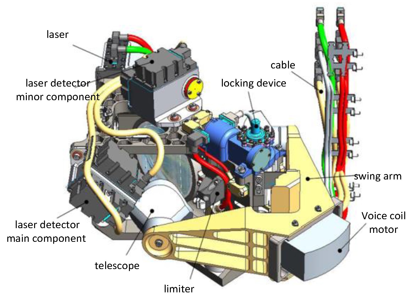
AIUS is a Michelson interferometer for measuring occultation transmittance spectra in the middle and upper atmosphere. Its interferometer model is depicted in
Figure 1. AIUS has the characteristics similar to those of ACE-FTS. Both instruments have a spectral resolution of 0.02 cm
−1. AIUS covers a spectral range from 750 cm
−1 to 4100 cm
−1, while ACE-FTS covers 750–4400 cm
−1. AIUS is a dual-band system composed of MCT (mercury cadmium telluride, 750–1850 cm
−1) and InSb (1850–4160 cm
−1). The instrument covers an altitude range from 8 to 100 km and has a field of view (FOV) of 1.25 mrad. A brief description of the two instruments is shown in
Table 1 [
4,
10].
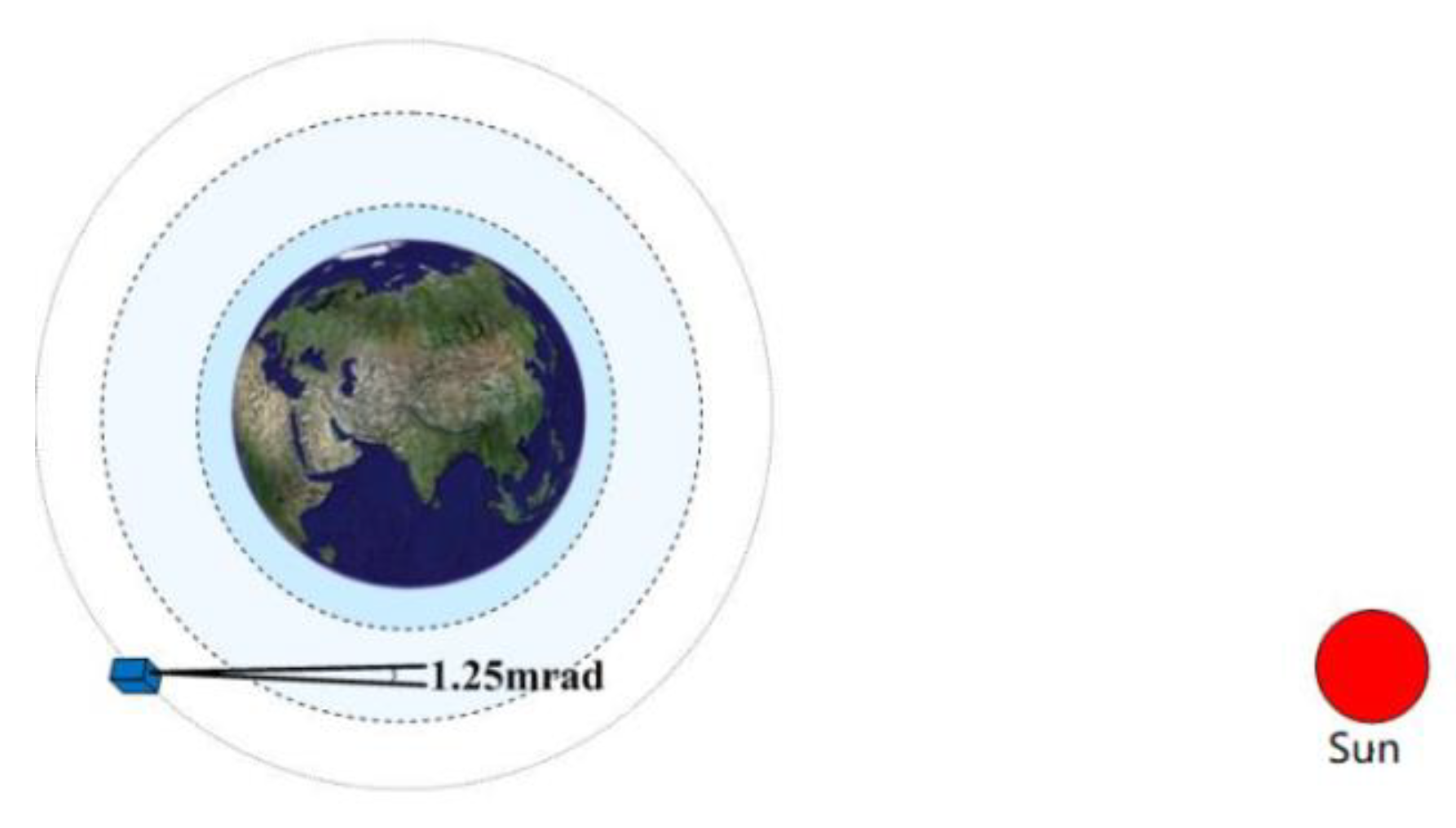
AIUS observes atmospheric parameters remotely by recording solar transmittance spectra as it tracks the Sun and scans through the atmosphere (see
Figure 2). The Sun tracking is carried out by a specific Sun-tracking camera. The position of the AIUS instrument is fixed. However, the center field of view of the AIUS can be adjusted using a two-dimensional pointing mechanism. The center position of the Sun is acquired using real-time processing of the Sun-tracking image, which is fed back to the two-dimensional pointing mechanism, and the pointing mechanism is adjusted so that the central field of view of the detector always points to the center position of the Sun. The uncertainty of the Sun-tracking is within 25 μrad [
10].
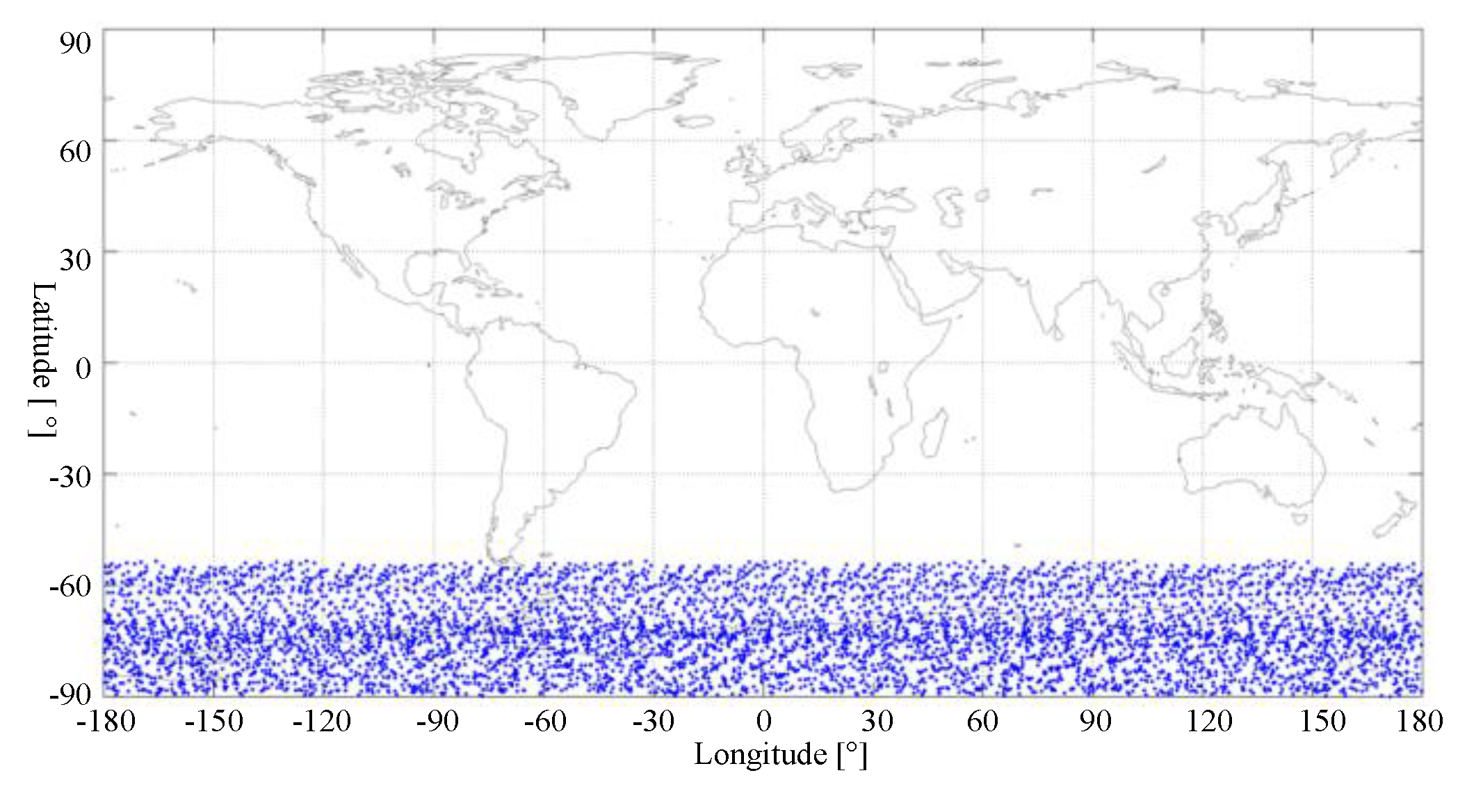
AIUS travels in a Sun-synchronous orbit and observes in a forward direction with a deviation angle from the along-track orbit. The deviation angle varies between 0 and 25°. The occultation spectra are scanned in an upward direction from the time of the Sun rising above the horizon to the time of the Sun moving out of the atmosphere. One orbit scan includes the measurements inside and outside of the atmosphere and the scan of deep space. It takes about two seconds in every scan at one tangent point. A scan sequence is acquired from the lowest altitude (about 8 km) to the highest altitude (about 100 km) in the atmosphere. Then, the sensor moves outside of the atmosphere and detects the solar spectra. Subsequently, the pointing mirror points to the deep space for producing the cold reference, which is used to calibrate the systematic errors. A complete orbit scan takes about three minutes. The measurements are repeated for each sunrise. AIUS measurements are mainly over the Antarctic.
Figure 3 shows the latitude coverage of AIUS that is between 55°S and 90°S.
2.2. Measurement Spectra
The GF5-AIUS level 0 data is the interferometric data in a binary format. The level 1 data is stored in HDF5 files and includes reconstructed spectra and processed auxiliary data. The AIUS level 0–1 processing includes four steps. The first step is the acquisition and processing of auxiliary data. By unpacking the auxiliary data package, information such as acquisition time, Sun position, and satellite position, is acquired. The geometric parameters, height and latitude and longitude coordinates, are calculated from the information of the Sun and satellite. The second step is to reconstruct the spectra from the original interferogram. However, the observed spectra can be contaminated by spikes that are related to the effect of energetic particles from space’s electromagnetic environment on orbits. The spike removal is considered in level 1 processing. Non-linear behavior of the detectors is expected and the corresponding correction is consolidated in-flight using data from the commissioning phase. After that, the FFT (fast Fourier transformation) is performed to compute the spectra. The third step is to evaluate the spectra’s quality using the standard deviation or mean value of the imaginary part of the calculated spectra by adding an additional quality flag. The wavelength calibration (750–4100 cm
−1) is carried out as well. First, the influence of the Doppler effect (the frequency shift) is removed, and a linear relationship between the sampling points of the Fourier transform spectrometer and the corresponding spectral coefficients is established. The subsequent spectral calibration is performed using a polynomial fitting method [
12,
13].
The last step of level 1 processing is to calculate the transmittance, which is directly obtained from DN (digital number) values. In addition to the observation of the Sun outside and inside the atmosphere, GF5-AIUS also observes deep space to remove the instrumental emission. Commonly, the transmittance
at tangent point
h can be calculated using the following equation:
where
,
, and
are the digital counts of the observation of the signal at tangent point
h, the solar radiation outside atmosphere, and the deep space signal, respectively.
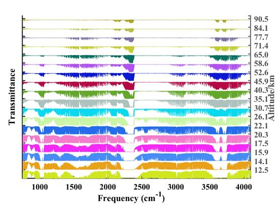
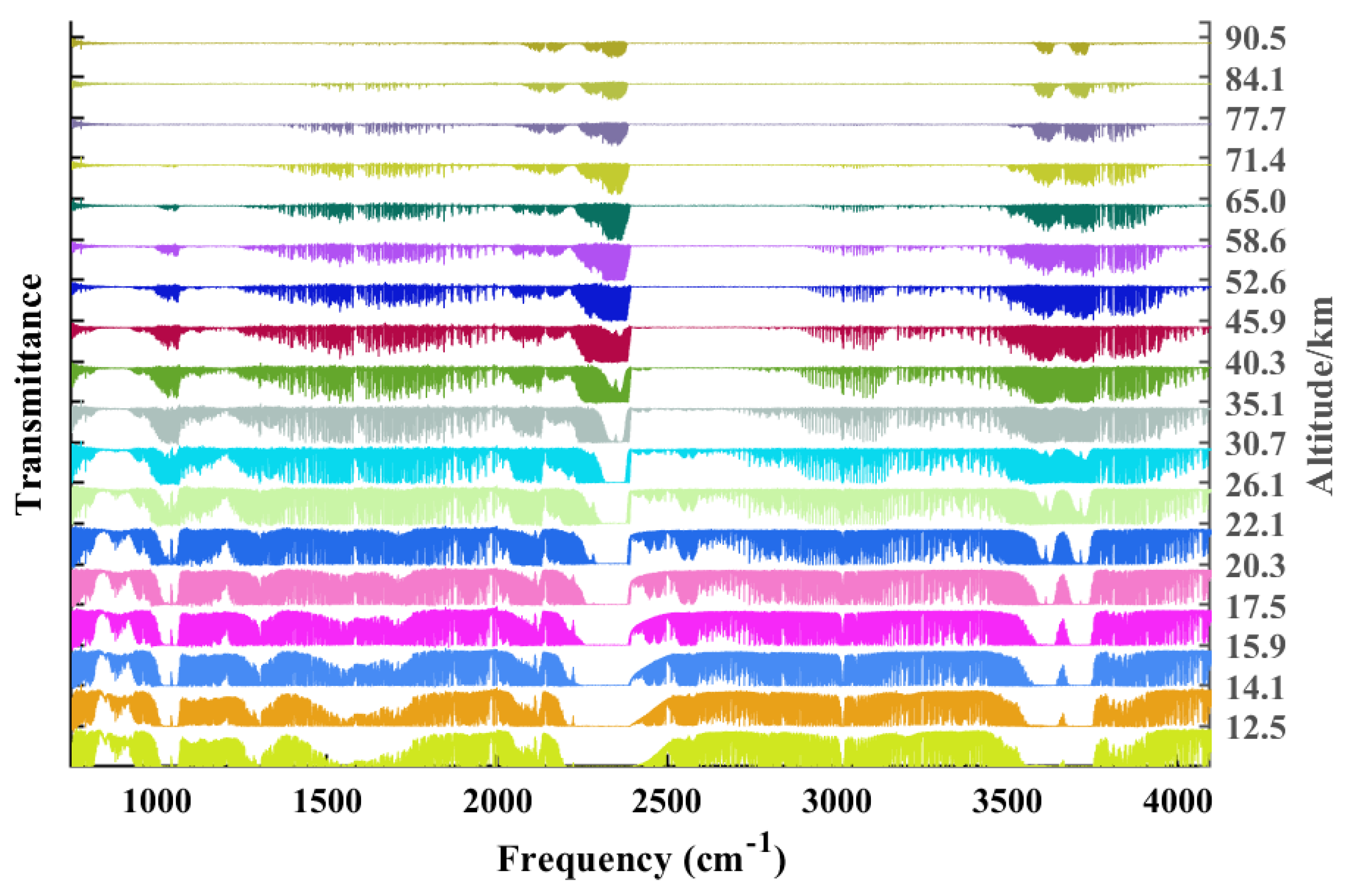
After about seven months of the in-orbit test, AIUS have been continuously providing measurement spectra.
Figure 4 shows AIUS spectra observed on 8 January 2019. To have a deeper understanding of the quality of the AIUS measurement spectra, the AIUS spectra are compared with the simulated spectra. The atmospheric profiles used in the simulation are adopted from the integrated atmospheric profiles, which will be described in
Section 3.3.
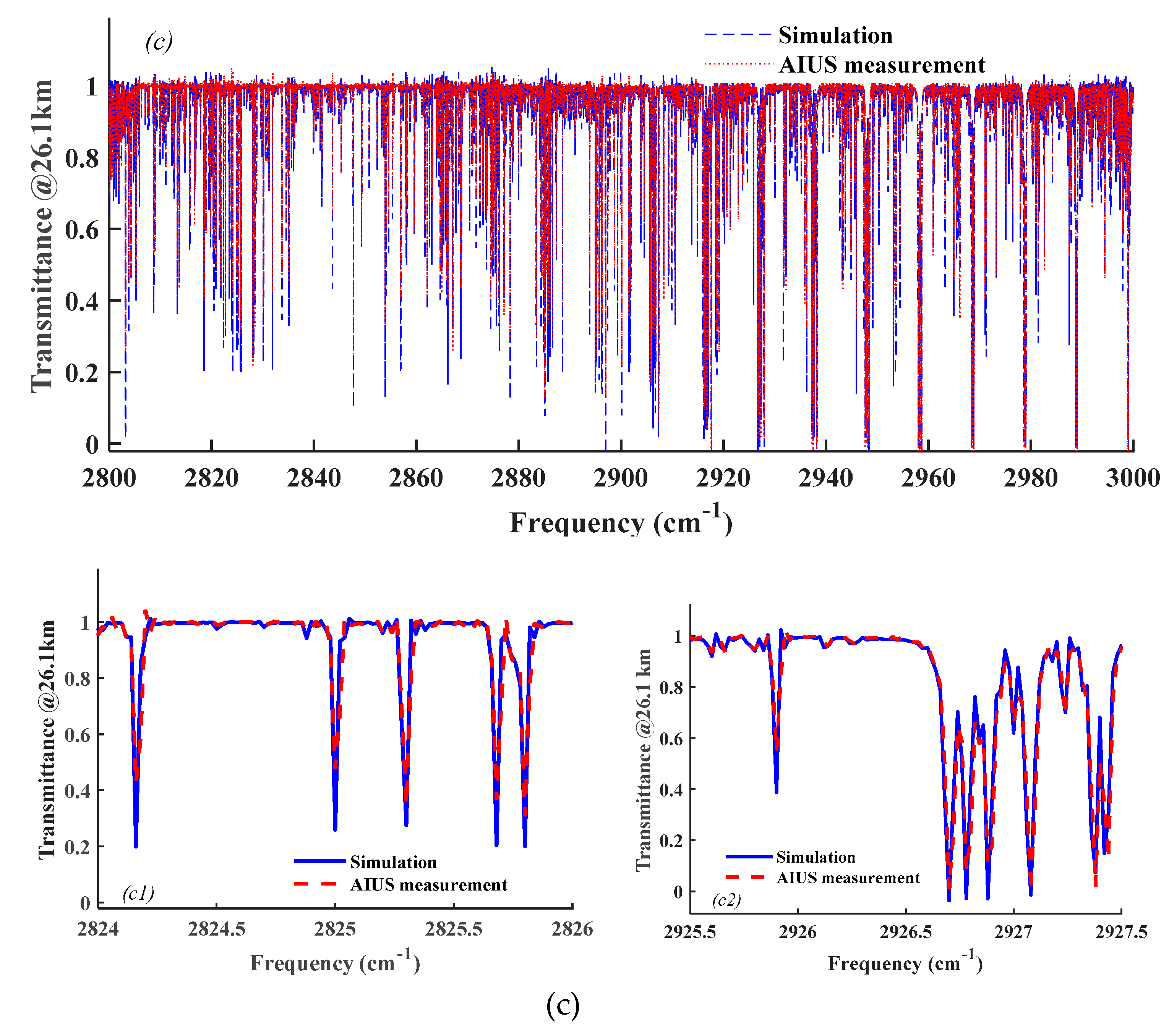
Figure 5 presents the comparison in the ranges of 1000–1200 cm
−1, 1400–1600 cm
−1, and 2800–3000 cm
−1, which are used for the retrieval of O
3, H
2O, and HCl, respectively.
Figure 5a shows the comparison between 1000 cm
−1 and 1200 cm
−1 at 33.4 km.
Figure 5b,c shows the spectra between 1400 cm
−1 and 1600 cm
−1 at 18.6 km and between 2800 cm
−1 and 3000 cm
−1 at 26.1 km, respectively. The zoom-in windows clearly illustrate that the AIUS measurement spectra agree well with the simulated spectra.
3. Retrieval Methodology of AIUS
Accurate knowledge of pointing and
p/
T (pressure/temperature) information is important for the high-precision quantitative retrieval of the abundances of atmospheric species from occultation-observed transmittances. The tangent height correction for AIUS is carried out by employing the triangular iteration with a tangential strides technique in a microwindow of N
2 continuum absorption. Details of the design and development of the tangent height correction algorithms are introduced in Zhu et al. [
14]. Details about the
p/
T retrieval will be introduced in a separate paper about a validation of
T profiles.
3.1. Spectral Microwindows of O3, H2O, and HCl
The spectral resolution of AIUS is about 0.02 cm−1. Because of this, the number of data points from each absorption band becomes unrealistic for an efficient inversion process. One should also avoid the effects from interfering chemical species for the retrieval of the target species to produce the best information from the retrieval. Thus, the retrieval is performed using a set of narrow spectral intervals (called “microwindows”) instead of an entire spectral band.
To select an appropriate set of microwindows, a sensitivity analysis with Jacobians is required. First of all, the spectral points that are sensitive to the target gas at each cutting height and are not sensitive to the interference gas according to the Jacobians of target and the interference species are selected. Then, the selected spectral points are increased on the basis of information entropy to generate a series of continuous window [
15]. Finally, all the selected spectral microwindows at every tangent height are combined.
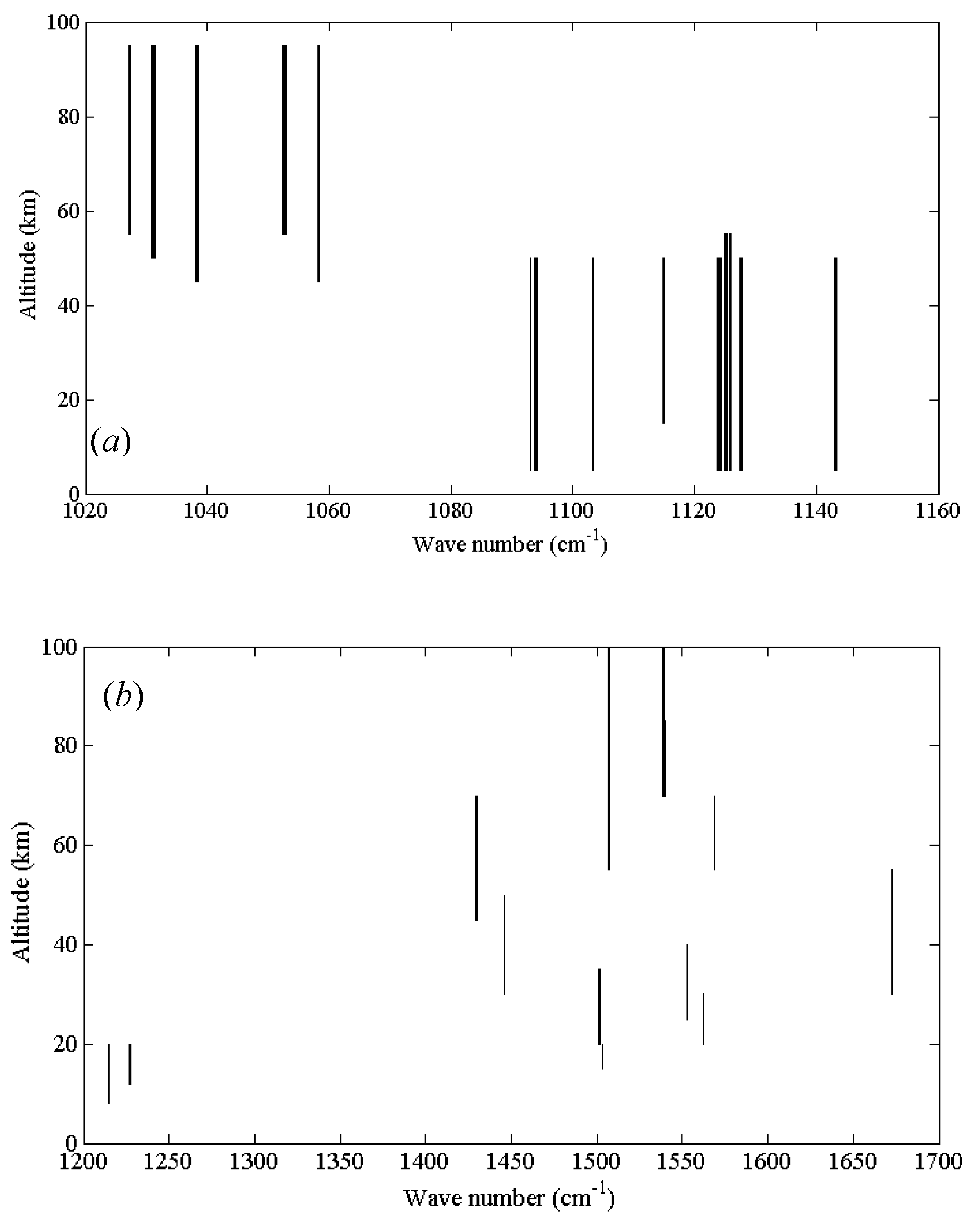
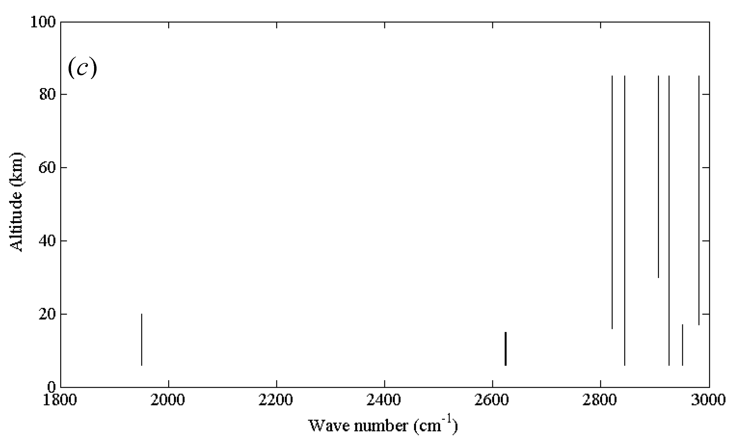
Figure 6 shows the selected microwindows for O
3, H
2O, and HCl retrievals, respectively. For O
3 retrieval, about 15 spectral microwindows are selected, covering from 5 to 95 km. The microwindows of 1020–1070 cm
−1 are more sensitive at higher altitudes, while others are more sensitive at lower altitudes. Thirteen spectral microwindows are selected for H
2O retrieval in the range of 1200–1700 cm
−1, covering about 8–100 km. Two spectral microwindows are found in 1200–1250 cm
−1 and 11 microwindows are found in 1400–1600 cm
−1. Eight spectral microwindows covering from 8 km to 85 km are selected for HCl, mainly in the range of 2800–3000 cm
−1. The microwindows for each retrieval target contains about 150–200 spectral points.
3.2. Inversion Model
Accurate modelling of the radiative transfer through the atmosphere plays an important role in the inversion. The forward model adopted in the retrieval algorithm of AIUS is the RFM (reference forward model) from Dudhia [
16], with the latest release being version v4.36 (
http://eodg.atm.ox.ac.uk/RFM/ index.html). Von Clarmann et al. [
17] have compared five forward models including the RFM. The inter-comparison experiment showed that an overall agreement between all models was reached, and RFM is proven to produce reliable simulations.
The inversion algorithm employed in this study is based on the OEM (optimal estimation method) proposed by Rodgers [
18]. The OEM retrieval framework has been widely applied to the inversion of atmospheric state parameters using infrared and microwave remote sensing measurements, with nadir, occultation, or limb viewing [
19,
20,
21,
22,
23,
24]. OEM stabilizes the inversion process by taking into account the statistical information about the atmospheric variability, which has been investigated by many studies [
25,
26,
27,
28,
29,
30,
31].
The inversion scheme uses the LM (Levenberg–Marquardt) method for solving the underlying least-squares fitting problem. By introducing a constraint factor γ, the next iteration is yielded using:
The inverse of the solution covariance in Equation (2) is given by:
The cost functions
is given by:
where
is the forward model,
is a vector of observations,
is the state of the atmosphere,
is the covariance matrix of the observation error, and
is the matrix of the weighting function. The
a priori state vector is denoted by
, with its covariance matrix
.
is the length of vector
.
In the AIUS retrieval scheme, the characteristics of AIUS have been fully taken into account when determining the factor γ and the covariance matrix
First, retrieval experiments are made based on many simulated spectra and AIUS observed spectra to decide an optimal
. After a statistical analysis, the factor of
is defined as a linear scaled function to the cost function and is updated at each iteration:
where
is a constant but changes for different atmospheric species.
The definition of the
a priori covariance matrix
follows Gaussian statistics and considers the correlation between different components of the state vector and the forward model vector [
31]. Different types of the correlation functions [
32] for computing the correlation have been tested based on the AIUS measurement spectra. In this study, we employed the linear correlation function:
where
i and
j are position indexes,
z is the position,
lc is the correlation length, and |*| signifies the absolute value. σ is the standard deviation calculated from the
a priori profiles.
3.3. Integrated Atmospheric Profiles
The forward model generates a numerical simulation of measurements based on the given atmospheric state. In other words, the accuracy of the simulated measurements depends on the reliability of the atmospheric parameters used in the forward model. In the retrieval scheme, a dataset of integrated atmospheric profiles based on MLS (Microwave Limb Sounder) level 2 products, ACE-FTS Climatology-Version 3.5 [
33], and the AFGL (Air Force Geophysics Laboratory) atmospheric models was generated.
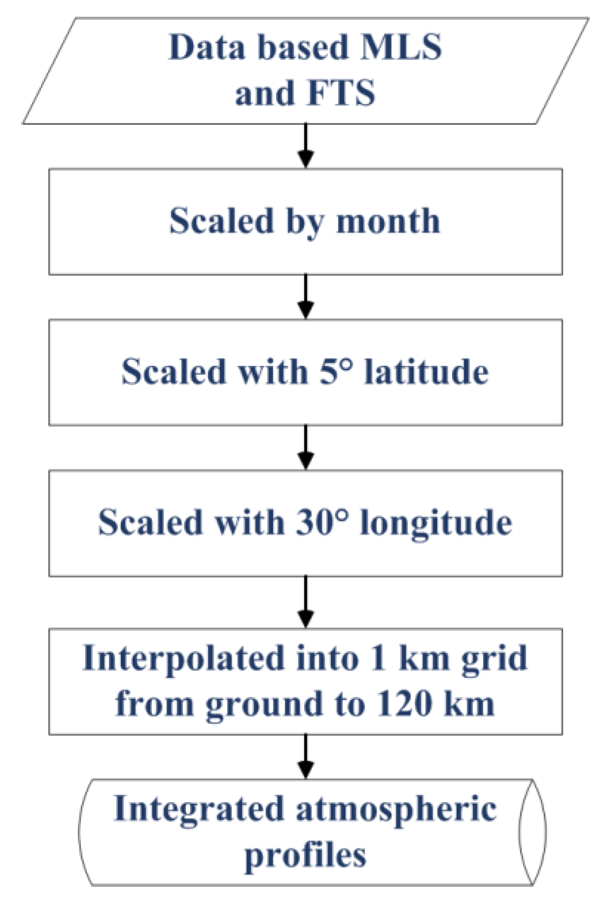
The MLS level 2 (v4.2) products between 2014 and 2016 were considered. The species profiles are classified and stored month by month for each set of products. Then, the monthly mean profiles are acquired and classified into different coordinate grids, which is discretized with a 5° latitude and 30° longitude spacing. That is, both of MLS and ACE-FTS datasets are classified by a monthly and geolocation grid. A diagram for constructing the integrated atmospheric profiles is shown in
Figure 7.
The next step was to combine the two sets of profiles. Since ACE-FTS and AIUS have similar instrument characteristics, the ACE-FTS product was chosen in the case that the profile of a particular species at the same geolocation and time can be found in both ACE-FTS and MLS datasets. Finally, the remaining species were read from the AFGL dataset. The profiles imported from the AFGL dataset include NH3, HBr, HI, PH3, H2S, F11, F12, F13, F21, F22, F114, F115, and HNO4. These species profiles from FASCOD (Fast Atmospheric Signature Code) Models 1–6 are resampled and integrated into the monthly geographic grids. In the end, the integrated atmospheric profiles dataset was produced.
4. Results
4.1. Assessment of the Retrieval Algorithm
Before performing the retrievals for the AIUS measurements, the retrieval experiments were carried out based on the simulated spectra and ACE-FTS measurements to test and verify our algorithm. We had no detailed parameters of ACE-FTS instrument, such as instrument line shape, the antenna response, etc. Thus, the parameters of AIUS were adopted to perform the retrieval experiments since the two instrument characteristics were similar. We adopted three ACE-FTS level 1 data sets to perform the O
3 retrieval experiments. Information of the ACE-FTS level-1 data used in this study is listed in
Table 2. All the
a priori profiles of O
3 and the other species were taken from the dataset of integrated atmospheric profiles described in
Section 3.3.
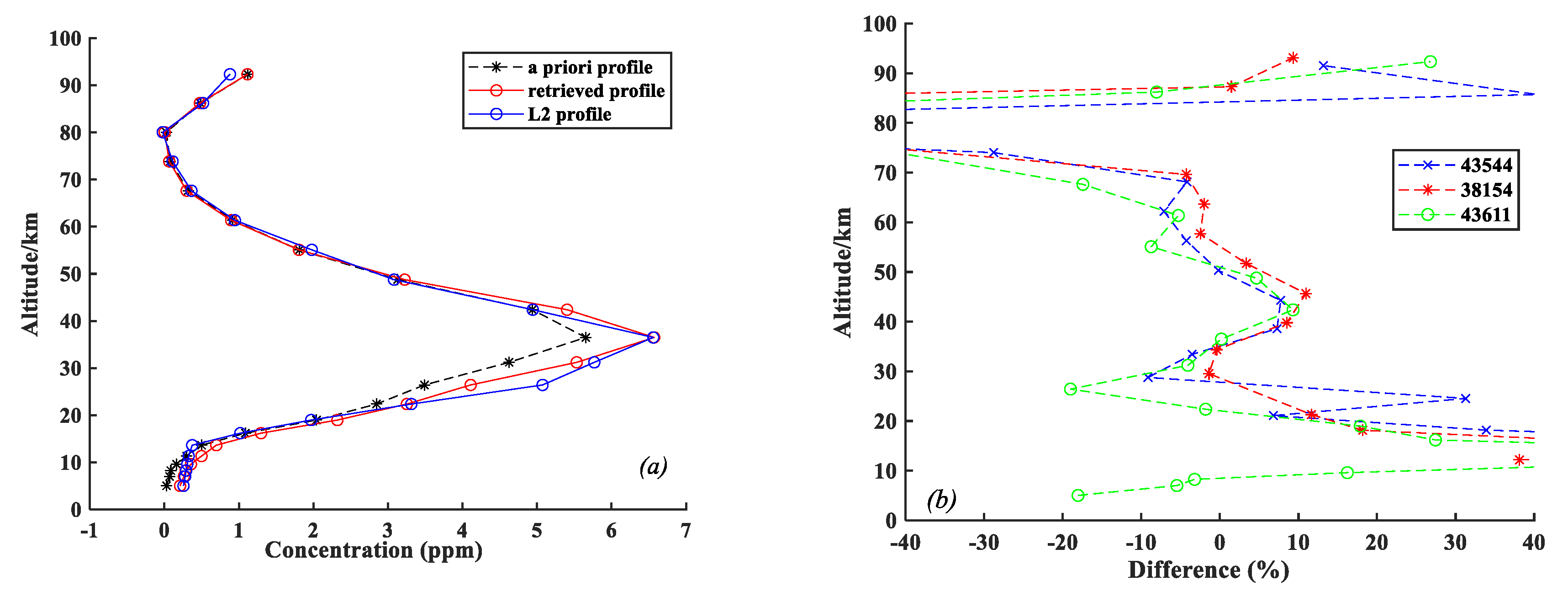
The retrieval profiles and the relative differences are shown in
Figure 8. The solid lines represent the O
3 profile retrieved by the AIUS retrieval algorithm and the dotted lines are ACE-FTS O
3 products, which were resampled to the retrieval grid. Only one pair of the retrieval and ACE-FTS official profiles is presented in
Figure 8a, indicating that the shape of the retrieval O
3 profiles agreed well with that of the ACE-FTS level 2 product. The relative difference in
Figure 8b illustrates that the relative difference between these three retrieval experiments was mostly within 10% between 20 km and 70 km for every pair of profiles, with some points reaching 15%–30%. The relative difference was larger below 20 km and over 70 km because of the uncertainties in the measurements. The bias of the ACE-FTS O
3 products was 1–8% in the stratosphere (16–44 km) and reached up to 40% (20% on average) above 45 km [
34,
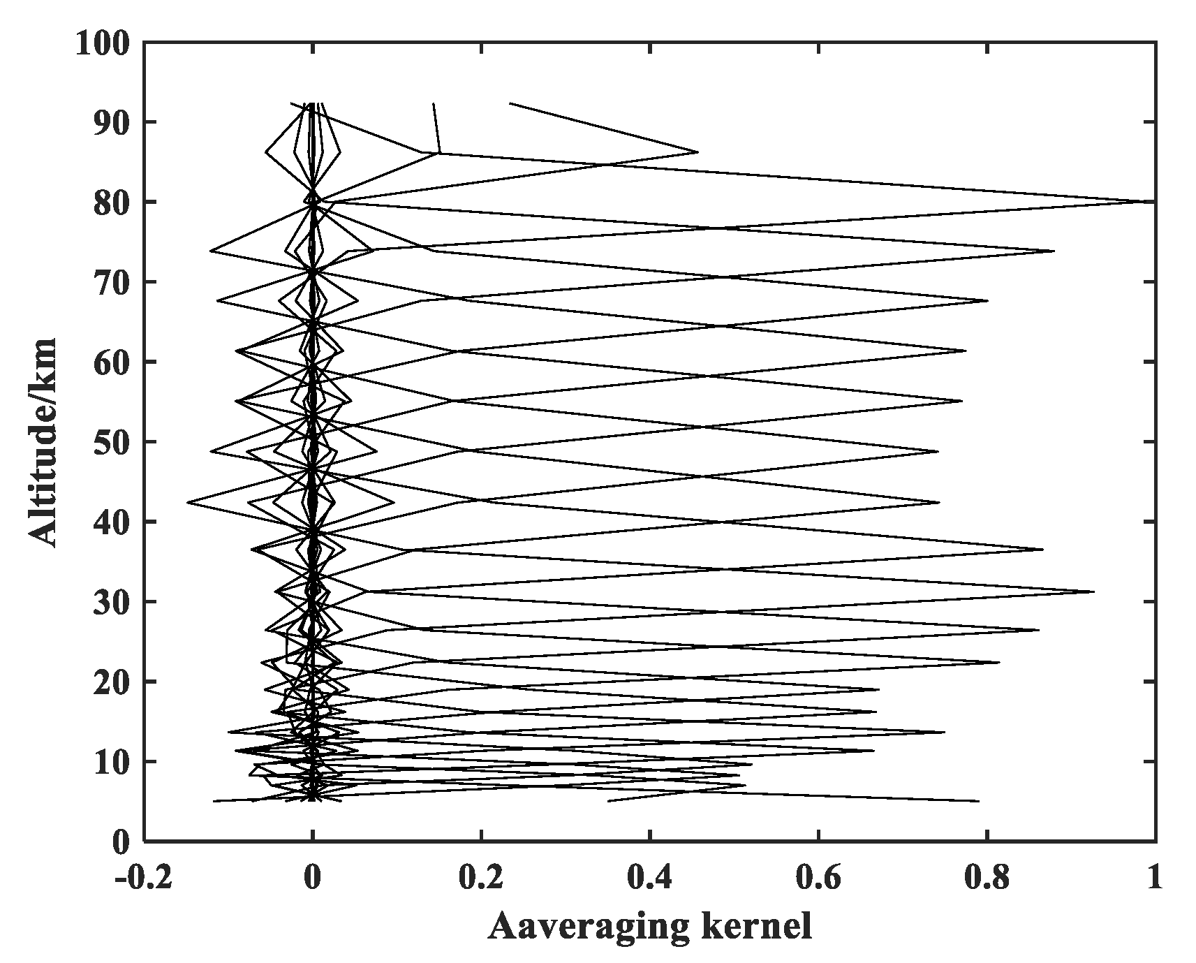
35]. The corresponding averaging kernels are plotted in
Figure 9, which reveal that the retrieval information mainly came from the measurements in the stratosphere. These retrieval experiments demonstrated that the performance of the retrieval algorithm was stable and delivered similar results compared to those official products using ACE-FTS data.
4.2. Retrieval from AIUS and Discussion
AIUS observes in a forward direction and scans one sequence (measurements from the lowest to the highest tangent altitudes) from one orbit. In this study, 24 orbital measurements were used to perform O
3, H
2O, and HCl retrievals. These 24 measurements were acquired during the period from 21 December 2018 to 8 January 2019. The orbit IDs of these measurements are 003301, 003331, 003337, 003341, 003344, 003366, 003367, 003370, 003372, 003385, 003387, 003399, 003403, 003416, 003424, 003429, 003435, 003458, 003479, 003480, 003487, 003489, 003504, and 003566. The latitudes of these measurements varied between 62.8°S and 65.5°S. The retrieval configurations are presented in
Table 3. The interfering molecules for O
3, H
2O, and HCl retrievals are also listed in
Table 3.
The retrieval profiles of AIUS are compared with the official AURA/MLS level-2 v4.2 profiles. All MLS profiles for comparisons were chosen according to their quality and convergence flags [
36]. In the AIUS retrieval configuration, the retrieval grid was identical to the tangent height grid, which means that the retrieval grid varied between these 24 measurements. So far, the effective altitudes of AIUS measurements are from about 12 to 90 km. For a comparison of the mean profiles, both retrieved AIUS and MLS profiles were resampled to the same altitude grids, from 12 km to 90 km with 2 km steps below 30 km and 3 km steps over 30 km. MLS products were represented as the mixing ratios versus pressure. The MLS altitudes were obtained from the geopotential height products.
4.2.1. O3 Retrieval Results and Comparisons
O
3 profiles were retrieved from the AIUS measurement spectra from 24 measurements and compared to the MLS O
3 profiles. Figure 11 shows a typical O
3 retrieval example based on AIUS measurements. According to the data quality document [
36] and validation of O
3 product version 2.2 [
41], the uncertainties of MLS O
3 profiles in the stratosphere are often about 5–10%, but over 20% when the atmospheric pressure is <0.1 hPa.
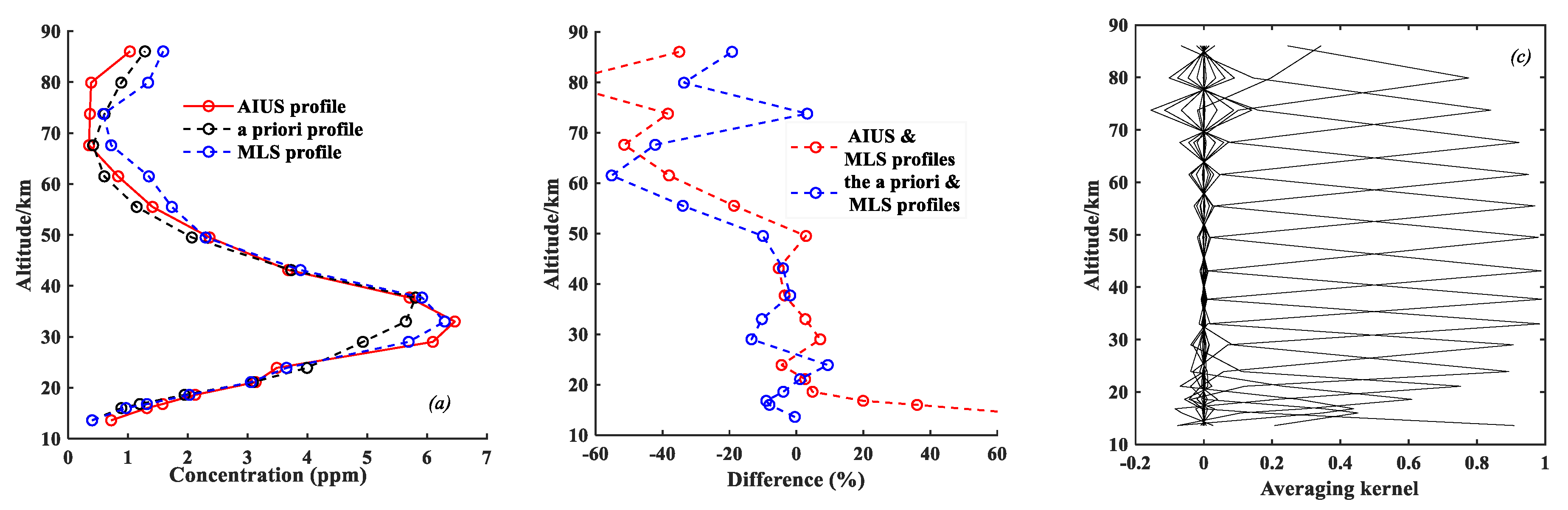
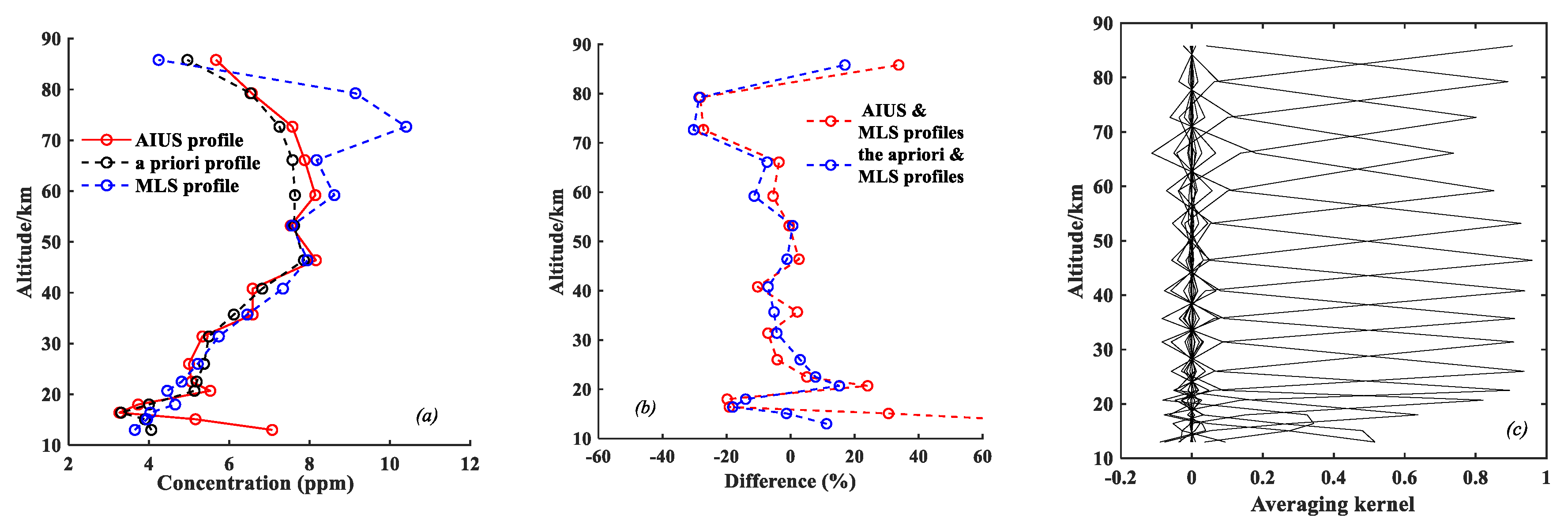
From the orbit 003301 measurement, the O
3 profile was retrieved between 12 km and 90 km. The retrieval of the AIUS O
3 profile is presented as a red line, the
a priori profile is shown as the black line, and the MLS profile is shown as the blue line, which was resampled to the retrieval grid.
Figure 10a shows that the retrieval AIUS O
3 profile was obviously different from the
a priori profile and agreed rather well with the MLS O
3 profile in the stratosphere. The relative difference between the retrieval and MLS O
3 products in
Figure 10b illustrates that the relative difference between the AIUS and MLS profiles was 3–8% between 18 and 50 km, 20–40% at 15–18 km, and mostly 20–40% from 55 km to 90 km, but occasionally greater than 40%. The relative difference between the
a priori and MLS profiles was within 15% below 50 km, and about 20–55% above 50 km.
Figure 10c is the retrieval averaging kernel for the orbit 003301 retrieval. The kernel reached about 0.8–1 at 20–80 km, which means that the retrieval information mainly came from the measurements.
O
3 profiles from 24 orbital AIUS measurements were retrieved. Since these measurements were all acquired near 65°S and over about 20 days, the comparison was made between the mean profile of the 24 pairs of AIUS and the equivalent MLS measurements.
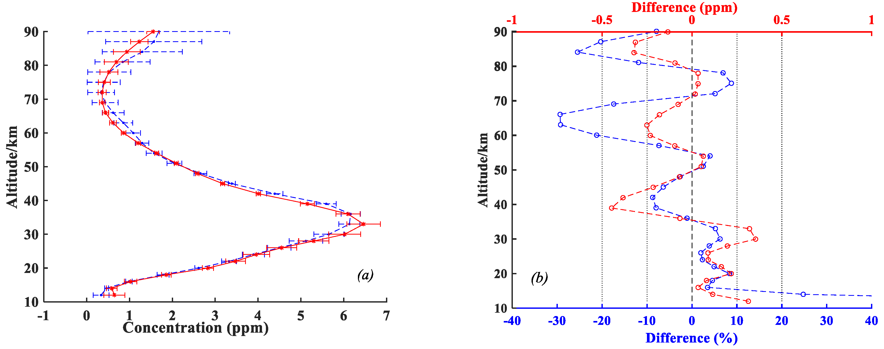
Figure 11a shows the mean profiles from AIUS and MLS with the corresponding standard deviations, which are shown as error bars. The standard deviations of the AIUS profiles were about 0.4 ppm between 30 and 40 km, which were bigger than those of the MLS profiles. This was because the two AIUS profiles retrieved from orbits 003504 and 003566 had lower peak values. The relative and absolute differences of the mean profiles of AIUS and MLS are presented in
Figure 11b. It indicates that the relative difference was within 10% (about 0.02–0.45 ppm) between 15 and 58 km, 20–30% for 60–70 km, and 80–90 km, respectively.
4.2.2. H2O Retrieval Results and Comparisons
The H
2O profiles were also retrieved from AIUS measurements and compared with MLS H
2O v4.2 profiles. For MLS H
2O v4.2 profiles, the accuracy was within 10% between 100 hPa and 0.1 hPa [
36]. An example of H
2O retrieval is presented in
Figure 12.
Figure 12a shows the AIUS H
2O,
a priori, and MLS H
2O profiles. The retrieval AIUS profile had a large deviation from the MLS profile between 70 and 80 km since the MLS profile had a sudden increase there. For this measurement pair, the relative difference between AIUS and MLS profile or between the
a priori and MLS profiles was mostly with 10% between 20 and 70 km, as can be seen from
Figure 12b. The averaging kernel in
Figure 12c indicates that the AIUS retrieval was mostly based on the measurement information, not the
a priori profile itself. The comparison of mean H
2O profiles between AIUS and MLS is shown in
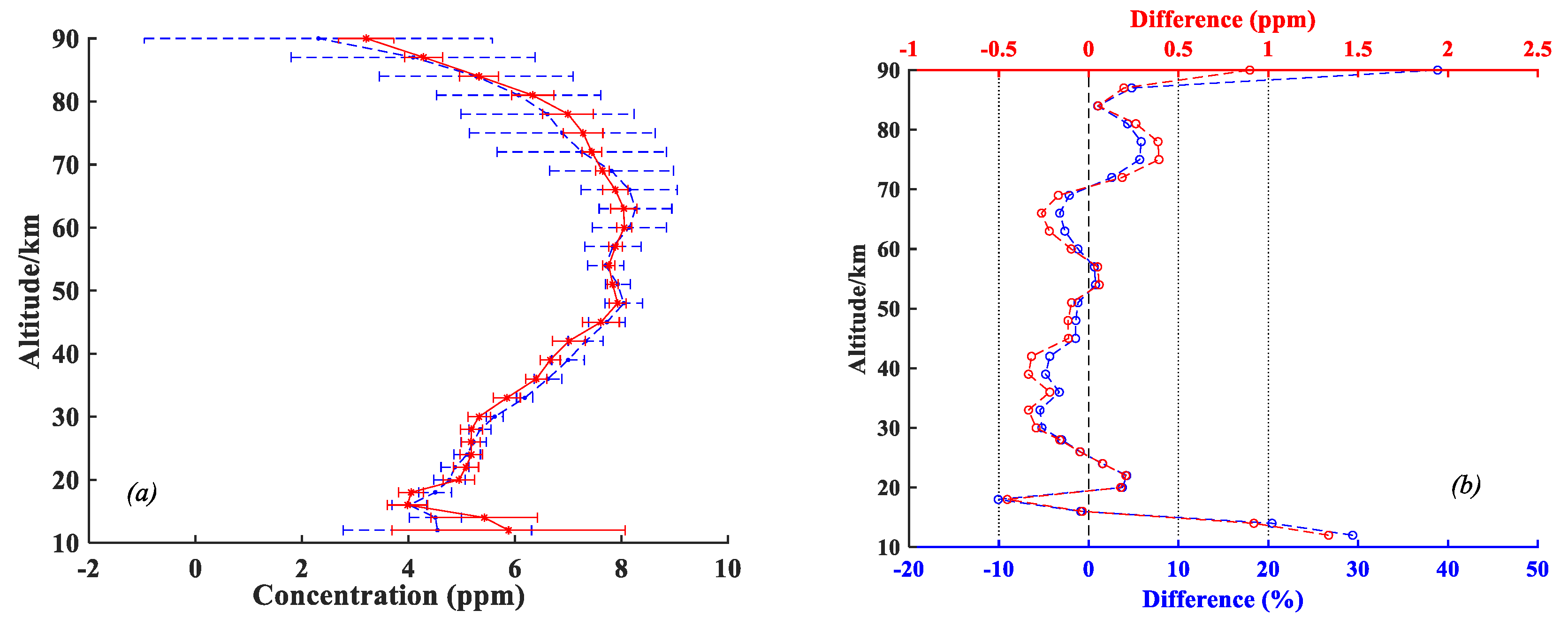
Figure 13. Only 23 pairs of AIUS and MLS profiles were used to make this comparison because the quality of the MLS profile from 8 January 2019, was below the required threshold. The mean AIUS H
2O profile had a good agreement with the mean MLS profile. The standard deviation of the AIUS profiles was greater than that of the MLS profiles below 20 km, while it was smaller between 70 and 90 km.
Figure 13b presents the absolute and relative differences between the AIUS and MLS profiles. The AIUS profiles mainly had a negative deviation from MLS profiles below 70 km. The relative difference was within 10% (0–0.5 ppm) between 15 and 80 km. However, the relative difference could reach 20–40% above 85 km and below 15 km.
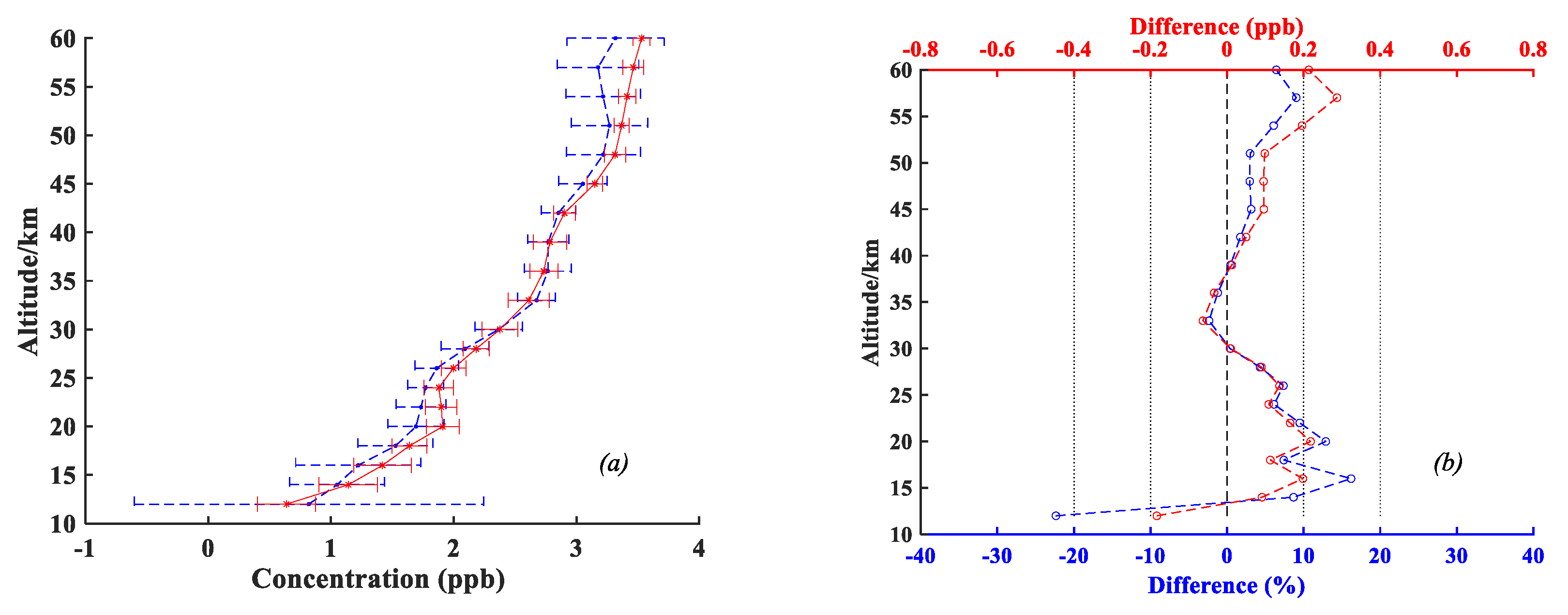
4.2.3. HCl Retrieval Results and Comparisons
Figure 14 and
Figure 15 present a typical HCl retrieval and the comparison of mean HCl profiles between AIUS and MLS. It has been reported that the accuracy of the MLS HCl v4.2 profiles is about 10% between 20 hPa and 0.32 hPa, and 10%–40% (occasionally more than 40%) between 100 hPa and 46 hPa [
36].
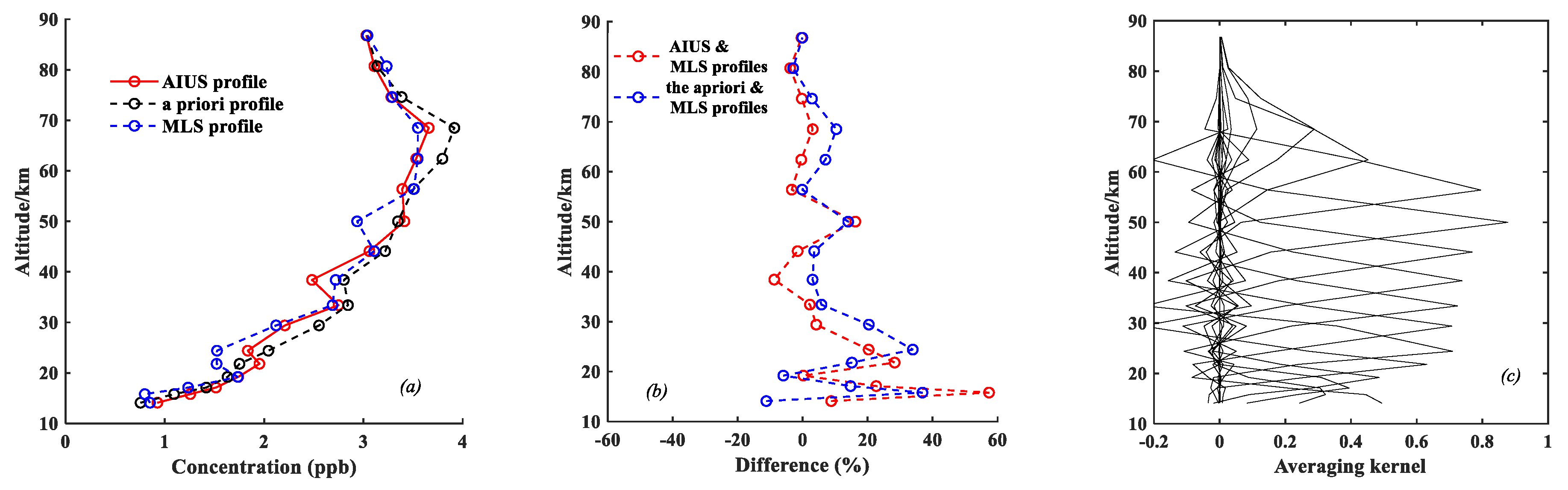
The AIUS and MLS HCl profiles in
Figure 14a capture a similar pattern.
Figure 14b illustrates that the difference between AIUS and MLS profiles was almost within 10% between 20 and 90 km, except for three altitude levels, which reached about 20%. The relative difference between the
a priori and MLS profiles was within 15% above 30 km and about 10–40% below 30 km. The averaging kernel below 60 km was about 0.5–0.8. However, it became wider above 60 km, which meant that the retrieval information mainly came from the
a priori profile. It is also reported by the official data quality document that MLS HCl profiles are unsuitable for scientific use over 0.32 hPa [
36]. Therefore, the comparison was made between 12 and 58 km (near 0.32 hPa).
Figure 15a shows the mean HCl profile and standard deviations of AIUS and MLS. The standard deviations are presented as error bars. The HCl profiles from the two instruments agreed quite well. The standard deviations of AIUS profiles (red solid line) became bigger below 20 km, while they were smaller at other altitudes.
Figure 15b indicates that the relative difference was within 10% (about 0–0.3 ppb) between 20 and 58 km, and was about 10–20% (about 0.2–0.35 ppb) between 10 and 20 km. AIUS HCl profiles mainly had a positive deviation from the MLS profiles between 15 and 58 km.
5. Discussion
ACE-FTS measurements were used for the assessment of the AIUS retrieval algorithm. The relative differences between the retrieval O3 profiles and the official ACE-FTS products were occasionally greater than 40% below 20 km and over 70 km. The main reason was that the bias of the official products at lower and higher altitudes was greater than those for the stratosphere. Another important reason is that the AIUS instrument parameters were used to retrieve the O3 profile from ACE-FTS measurements, and the uncertainty in the AIUS parameterization can affect the retrieval.
The profiles retrieved from the AIUS measurement were all above 10 km since the quality of the measurements below 10 km were unacceptable because of the large noise level. The comparisons between the AIUS and MLS retrievals showed that the AIUS O3 profiles agreed well with the MLS profiles between 15 km and 58 km, while larger differences could mostly be found above 60 km. One reason for the larger relative difference above 60 km may be the larger uncertainties of the MLS profile above 60 km. Another important reason is that the AIUS measurements had a large noise level above 60 km in the ozone fitting microwindows. AIUS observes the atmosphere during the sun rising. The local times of the 24 orbital AIUS observed spectra were about 2:00. However, some MLS profiles’ local times were about 0:40, while the others were about 15:00. Thus, one more possible reason for these uncertainties may be the diurnal variation of O3, since the acquisition local times of some pairs of AIUS and MLS were different.
The comparisons also revealed that the AIUS retrievals had larger uncertainties at lower altitudes for the O
3, H
2O, and HCl profiles. One possible factor would be that both retrievals were insensitive to the measurement information in the troposphere and mainly relied on the
a priori profile, which can be seen using the averaging kernel at lower altitudes in
Figure 10,
Figure 12, and
Figure 14. Another reason might be the uncertainties introduced by the interfering species profiles. One more reason might come from the tangent height correction, which had larger uncertainties below 15 km. Nevertheless, the quality of the AIUS observed spectra can still be improved as the level 1 processing is currently under an optimized level.
6. Conclusions
This study has introduced a retrieval algorithm developed for an infrared occultation spectrometer called AIUS, which is on board the Chinese GaoFen-5 satellite. For the first time, O3, H2O, and HCl profiles were retrieved from AIUS observed spectra, and the retrieved profiles were compared with the official AURA/MLS Level-2 products.
Before performing retrievals from real AIUS measurements, the retrieval experiments were carried out to assess the retrieval algorithm based on ACE-FTS measurements. The experiments demonstrate that the retrieval algorithm is reliable and works effectively.
O3, H2O, and HCl retrievals were performed using AIUS 24 orbital measurements. The comparisons between AIUS and MLS indicated that the relative difference was within 10% at 18–58 km for O3 profiles, within 10% at 15–80 km for H2O profiles, and within 10% at 30–60 km and 10–20% at 16–30 km for HCl profiles.
In future work, further studies are required to improve the data quality of the AIUS measurements at low altitudes. The retrieval algorithm will be improved as well and more trace gases, such as CH4, CO2, OCS, etc., will be retrieved. In addition, the influence of interfering species on the retrieval will be probed. An extensive retrieval error characterization will be analyzed. Further validations will be performed by comparing between MLS and other datasets using large amounts of measurement spectra over an extensive temporal and spatial range.
Author Contributions
Conceptualization, X.L. and T.C.; Formal analysis, H.W., S.Z., J.M., and Q.L.; Funding acquisition, X.L.; Investigation, J.X. and H.S.; Methodology, X.L.; Resources, X.Z. and S.G.; Writing—original draft, X.L.; Writing—review and editing, J.X.
Funding
This research was funded by National Natural Science Foundation of China under grant 41571345, the National Key Research and Development Program of China under grant 2016YFB0500705, and the Major Projects of High Resolution Earth Observation System under grant 32-Y20A18-9001-15-17-1.
Acknowledgments
Pengmei Xu and her research team provided the AIUS parameters and helped with the raw data of AIUS. The ACE-FTS data were provided by ACE-FTS team. ACE, also known as SCISAT, is a Canadian-led mission mainly supported by the Canadian Space Agency (CSA). Thanks are also given to Professor Anu Dudhia for providing the RFM source code and help.
Conflicts of Interest
The authors declare no conflict of interest.
References
- Manney, G.L.; Santee, M.L.; Livesey, N.J.; Froidevaux, L.; Read, W.G.; Pumphrey, H.C.; Waters, J.W.; Pawson, S. EOS Microwave Limb Sounder observation of the Antarctic polar vortex breakup in 2004. Geophys. Res. Lett. 2005, 32, 1–5. [Google Scholar] [CrossRef]
- Santee, M.L.; Manney, G.L.; Livesey, N.J.; Froidevaux, L.; MacKenzie, I.A.; Pumphrey, H.C.; Read, W.G.; Schwartz, M.J.; Waters, J.W.; Harwood, R.S. Polar processing and development of the 2004 Antarctic ozone hole: First results from MLS on Aura. Geophys. Res. Lett. 2005, 32, 1–4. [Google Scholar] [CrossRef]
- Gattinger, R.L.; McDade, I.C.; Alfaro Suzan, A.L.; Boone, C.D.; Walker, K.A.; Bernath, P.F.; Evans, W.F.J.; Degenstein, D.A.; Yee, J.H.; Sheese, P.; et al. NO2 air afterglow and O and NO densities from Odin-OSIRIS night and ACE-FTS sunset observations in the Antarctic MLT region. J. Geophys. Res. 2010, 115, 1256–1268. [Google Scholar] [CrossRef]
- Bernath, P.F.; McElroy, C.T.; Abrams, M.C.; Boone, C.D.; Butler, M.; Camy-Peyret, C.; Carleer, M.; Clerbaux, C.; Coheur, P.-F.; Colin, R.; et al. Atmospheric Chemistry Experiment (ACE): Mission overview. Geophys. Res. Lett. 2005, 32. [Google Scholar] [CrossRef]
- Fischer, H.; Birk, M.; Blom, C.; Carli, B.; Carlotti, M.; von Clarmann, T.; Delbouille, L.; Dudhia, A.; Ehhalt, D.; Endemann, M.; et al. MIPAS: An instrument for atmospheric and climate research. Atmos. Chem. Phys. 2008, 8, 2151–2188. [Google Scholar] [CrossRef]
- Russell, J.M.; Gordley, L.L.; Park, J.H.; Drayson, S.R.; Hesketh, W.D.; Cicerone, R.J.; Tuck, A.F.; Frederick, J.E.; Harries, J.E.; Crutzen, P.J. The Halogen Occultation Experiment. J. Geophys. Res. Atmos. 1993, 98, 10777–10797. [Google Scholar] [CrossRef]
- Gunson, M.R.; Abbas, M.M.; Abrams, M.C.; Allen, M.; Brown, L.R.; Brown, T.L.; Chang, A.Y.; Goldman, A.; Irion, F.W.; Lowes, L.L.; et al. The Atmospheric Trace Molecule Spectroscopy (ATMOS) experiment: Deployment on the ATLAS Space Shuttle missions. Geophys. Res. Lett. 1996, 23, 2333–2336. [Google Scholar] [CrossRef]
- Bovensmann, H.; Burrows, J.P.; Buehwitz, M.; Frerick, J.; Noel, S.; Rozanov, V.V. SCIAMACHY: Mission Objectives and Measurement Modes. J. Atmos. Sci. 1999, 56, 127–150. [Google Scholar] [CrossRef] [Green Version]
- Beer, R.; Glavich, T.A.; Rider, D.M. Tropospheric emission spectrometer for the Earth Observing System’s Aura Satellite. Appl. Opt. 2001, 40, 2356–2367. [Google Scholar] [CrossRef]
- Wang, H.; Li, X.; Xu, J.; Zhang, X.; Ge, S.; Chen, L.; Wang, Y.; Zhu, S.; Miao, J.; Si, Y. Assessment of Retrieved N2O, NO2, and HF Profiles from the Atmospheric Infrared Ultraspectral Sounder Based on Simulated Spectra. Sensors 2018, 18, 2209. [Google Scholar] [CrossRef]
- Dong, X.; Xu, P.M.; Hou, L.Z. Design and Implementation of Atmospheric Infrared Ultra-spectral Sounder. Spacecr. Recovery Remote Sens. 2018, 39, 29–37. [Google Scholar]
- Dutil, Y.; Lantagne, S.; Dubé, S.; Poulin, R. ACE-FTS Level 0 To 1 Data Processing, Earth Observing Systems VII. In Proceedings of the SPIE, Seattle, WA, USA, 24 September 2002; Volume 4814, pp. 102–110. [Google Scholar]
- Worden, H.; Beer, R.; Bowman, K.W.; Fisher, B.; Luo, M.Z.; Rider, D.; Sarkissian, E.; Tremblay, D.; Zong, J. TES level 1 algorithms: Interferogram processing, geolocation, radiometric, and spectral calibration. IEEE Trans. Geosci. Remote Sens. 2006, 44, 1288–1296. [Google Scholar] [CrossRef]
- Zhu, S.Y.; Li, X.Y.; Xu, J.; Cheng, T.H.; Zhang, X.Y.; Wang, H.M.; Wang, Y.P.; Miao, J. Neural network aided fast pointing information determination approach for occultation payloads from in-flight measurements: Algorithm design and assessment. Adv. Space Res. 2019, 63, 2323–2336. [Google Scholar] [CrossRef]
- Kuai, L.; Natraj, V.; Shia, R.L.; Miller, C.; Yung, Y.L. Channel selection using information content analysis: A case study of CO2 retrieval from near infrared measurements. J. Quant. Spectrosc. Radiat. Transf. 2010, 111, 1296–1304. [Google Scholar] [CrossRef]
- Dudhia, A. The Reference Forward Model (RFM). J. Quant. Spectrosc. Radiat. Transf. 2017, 186, 243–253. [Google Scholar] [CrossRef] [Green Version]
- Von Clarmann, T.; Hopfner, M.; Funke, B.; Lopez-Puertas, M.; Dudhia, A.; Jay, V.; Schreier, F.; Ridolfi, M.; Ceccherini, S.; Kerridge, B.J.; et al. Modelling of atmospheric mid-infrared radiative transfer: The AMIL2DA algorithm intercomparison experiment. J. Quant. Spectrosc. Radiat. Transf. 2003, 78, 381–407. [Google Scholar] [CrossRef]
- Rodgers, C.D. Retrieval of atmospheric temperature and composition from remote measurements of thermal radiation. Rev. Geophys. Space Phys. 1976, 14, 609–624. [Google Scholar] [CrossRef]
- Urban, J.; Baron, P.; Lautie, N.; Schneider, N.; Dassas, K.; Ricaud, P.; de la Noë, J. Moliere (v5): A versatile forward- and inversion model for the millimeter and sub-millimeter wavelength range. J. Quant. Spectrosc. Radiat. Transf. 2004, 83, 529–554. [Google Scholar] [CrossRef]
- Boone, C.D.; Nassar, R.; Walker, K.A.; Rochon, Y.; McLeod, S.D.; Rinsland, C.P.; Bernath, P.F. Retrievals for the atmospheric chemistry experiment Fourier-transform spectrometer. Appl. Opt. 2005, 44, 7218–7231. [Google Scholar] [CrossRef] [Green Version]
- Raspollini, P.; Belotti, C.; Burgess, A.; Carli1, B.; Carlotti, M.; Ceccherini, S.; Dinelli, B.M.; Dudhia, A.; Flaud, J.M.; Funke, B.; et al. MIPAS level 2 operational analysis. Atmos. Chem. Phys. 2006, 6, 5605–5630. [Google Scholar] [CrossRef] [Green Version]
- Livesey, N.J.; Snyder, W.V.; Read, W.G.; Wagner, P.A. Retrieval Algorithms for the EOS Microwave Limb Sounder (MLS). IEEE Trans. Geosci. Remote Sens. 2006, 44, 1144–1155. [Google Scholar] [CrossRef]
- Bowman, K.W.; Rodgers, C.D.; Kulawik, S.S.; Worden, J.; Sarkissian, E.; Osterman, G.; Steck, T.; Lou, M.; Eldering, A.; Shephard, M.; et al. Tropospheric Emission Spectrometer: Retrieval Method and Error Analysis. IEEE Trans. Geosci. Remote Sens. 2006, 44, 1297–1307. [Google Scholar] [CrossRef]
- Takahashi, C.; Ochiai, S.; Suzuki, M. Operational retrieval algorithms for JEM/SMILES level 2 data processing system. J. Quant. Spectrosc. Radiat. Transf. 2010, 111, 160–173. [Google Scholar] [CrossRef]
- Rodgers, C.D. Inverse Methods for Atmospheric Sounding: Theory and Practice, Series on Atmospheric Oceanic and Planetary Physics-Vol. 2; World Scientific Publishing Co. Pte. Ltd.: Farrer Road, Singapore, 2000; pp. 92–93. ISBN 981-02-2740-X. [Google Scholar]
- Eriksson, P. Analysis and comparison of two linear regularization methods for passive atmospheric observations. J. Geophys. Res. 2000, 105, 18157–18167. [Google Scholar] [CrossRef]
- Doicu, A.; Schreier, F.; Hess, M. Iteratively regularized Gauss—Newton method for atmospheric remote sensing. Comput. Phys. Commun. 2002, 148, 214–226. [Google Scholar] [CrossRef]
- Steck, T. Methods for determining regularization for atmospheric retrieval problems. Appl. Opt. 2002, 41, 1788–1797. [Google Scholar] [CrossRef] [PubMed]
- Jiang, D.M.; Dong, C.H. A review of optimal algorithm for physical retrieval of atmospheric profile. Adv. Earth Sci. 2010, 25, 133–139. [Google Scholar]
- Zou, M.M.; Chen, L.F.; Li, S.S.; Fan, M.; Tao, J.H.; Zhang, Y. An improved constraint method in optimal estimation of CO2 from GOSAT SWIR observations. Sci. China Earth Sci. 2016. [Google Scholar] [CrossRef]
- Xu, J.; Schreier, F.; Doicu, A.; Trautmann, T. Assessment of Tikhonov-type regularization methods for solving atmospheric inverse problems. J. Quant. Spectrosc. Radiat. Transf. 2016, 184, 274–286. [Google Scholar] [CrossRef] [Green Version]
- Eriksson, P.; Jimeneza, C.; Buehler, S.A. Qpack, a general tool for instrument simulation and retrieval work. J. Quant. Spectrosc. Radiat. Transf. 2005, 91, 47–64. [Google Scholar] [CrossRef]
- Koo, J.H.; Walker, K.A.; Jones, A.; Sheese, P.E.; Boone, C.D.; Bernath, P.F.; Manney, G.L. Global climatology based on the ACE-FTS version 3.5 data set: Addition of mesospheric levels and carbon-containing species in the UTLS. J. Quant. Spectrosc. Radiat. Transf. 2017, 12, 52–62. [Google Scholar] [CrossRef]
- Jones, A.; Walker, K.A.; Jin, J.J.; Taylor, J.R.; Boone, C.D.; Bernath, P.F.; Brohede, S.; Manney, G.L.; McLeod, S.; Hughes, R.; et al. Technical Note: A trace gas climatology derived from the Atmospheric Chemistry Experiment Fourier Transform Spectrometer (ACE-FTS) data set. Atmos. Chem. Phys. 2012, 12, 5207–5220. [Google Scholar] [CrossRef] [Green Version]
- Dupuy, E.; Walker, K.A.; Kar, J.; Boone, C.D.; McElroy, C.T.; Bernath, P.F.; Drummond, J.R.; Skelton, R.; McLeod, S.D.; Hughes, R.C.; et al. Validation of ozone measurements from the atmospheric Chemistry Experiment (ACE). Atmos. Chem. Phys. 2009, 9, 287–343. [Google Scholar] [CrossRef]
- Livesey, N.J.; Read, W.G.; Wagner, P.A.; Froidevaux, L.; Lambert, A.; Manney, G.L.; Mill´an Valle, L.F.; Pumphrey, H.C.; Santee, M.L.; Schwartz, M.J.; et al. Version 4.2x Level 2 Data Quality and Description Document. JPL D-33509 Rev. B; 2016. Available online: http://mls.jpl.nasa.gov/ (accessed on 21 February 2017).
- Gordon, I.E.; Rothman, L.S.; Hill, C.; Kochanov, R.V.; Tan, Y.; Bernath, P.F.; Birk, M.; Boudon, V.; Campargue, A.; Chance, K.V.; et al. The HITRAN2016 Molecular Spectroscopic Database. J. Quant. Spectrosc. Radiat. Transf. 2017, 203, 3–69. [Google Scholar] [CrossRef]
- Mlawer, E.J.; Payne, V.H.; Moncet, J.L.; Delamere, J.S.; Alvarado, M.J.; Tobin, D.C. Development and recent evaluation of the MT-CKD model of continuum absorption. Philos. Trans. R. Soc. A Math. Phys. Eng. Sci. 2012, 370, 2520–2556. [Google Scholar] [CrossRef] [PubMed]
- Thibault, F.; Menoux, V.; Le Doucen, R.; Rosenmann, L.; Hartmann, J.M.; Boulet, C. Infrared collision-induced absorption by O2 near 6.4 µm for atmospheric applications: Measurements and empirical modeling. Appl. Opt. 1997, 36, 563–567. [Google Scholar] [CrossRef]
- Lafferty, W.J.; Solodov, A.M.; Weber, A.; Olson, W.B.; Hartmann, J.M. Infrared collision-induced absorption by N2 near 4.3 µm for atmospheric applications: Measurements and empirical modeling. Appl. Opt. 1996, 35, 5911–5917. [Google Scholar] [CrossRef] [PubMed]
- Froidevaux, L.; Jiang, Y.B.; Lambert, A.; Livesey, N.J.; Read, W.G.; Waters, J.W.; Browell, E.V.; Hair, J.W.; Avery, M.A.; McGee, T.J.; et al. Validation of Aura Microwave Limb Sounder stratospheric ozone. measurements. J. Geophys. Res. Atmos. 2008, 113. [Google Scholar] [CrossRef]
Figure 1.
AIUS interferometer model [
11].
Figure 1.
AIUS interferometer model [
11].
Figure 2.
AIUS measurement geometry.
Figure 2.
AIUS measurement geometry.
Figure 3.
The coverage of AIUS measurements.
Figure 3.
The coverage of AIUS measurements.
Figure 4.
AIUS measurements spectra at 64.7°S, 142.5°W on 8 January 2019.
Figure 4.
AIUS measurements spectra at 64.7°S, 142.5°W on 8 January 2019.
Figure 5.
The comparison between AIUS measurement spectra and the simulated spectra. (a) Spectra (1000–1200 cm−1) at 63.5°S6.9°E on 1 January 2019; (b) Spectra (1400–1600 cm−1) at 63°S80°W on 21 December 2018; (c) Spectra (2800–3000 cm−1) at 64.7°S142.48°W on 1 January 2019.
Figure 5.
The comparison between AIUS measurement spectra and the simulated spectra. (a) Spectra (1000–1200 cm−1) at 63.5°S6.9°E on 1 January 2019; (b) Spectra (1400–1600 cm−1) at 63°S80°W on 21 December 2018; (c) Spectra (2800–3000 cm−1) at 64.7°S142.48°W on 1 January 2019.
Figure 6.
The spectral microwindows: (a) O3, (b) H2O, and (c) HCl.
Figure 6.
The spectral microwindows: (a) O3, (b) H2O, and (c) HCl.
Figure 7.
Process of constructing the integrated atmospheric profiles.
Figure 7.
Process of constructing the integrated atmospheric profiles.
Figure 8.
O3 retrieval experiment based on ACE-FTS spectra: (a) retrieval and ACE-FTS L2 profiles (ID 43611), and (b) relative difference between retrieval and FTS L2 products.
Figure 8.
O3 retrieval experiment based on ACE-FTS spectra: (a) retrieval and ACE-FTS L2 profiles (ID 43611), and (b) relative difference between retrieval and FTS L2 products.
Figure 9.
A typical averaging kernel for the O3 retrieval from ACE-FTS spectra.
Figure 9.
A typical averaging kernel for the O3 retrieval from ACE-FTS spectra.
Figure 10.
O3 retrieval from AIUS measurements on orbit 003301: (a) retrieval, a priori, and MLS L2 profiles; (b) relative difference between the retrieval and MLS L2 profiles, and the a priori and MLS L2 profiles; and (c) the averaging kernel.
Figure 10.
O3 retrieval from AIUS measurements on orbit 003301: (a) retrieval, a priori, and MLS L2 profiles; (b) relative difference between the retrieval and MLS L2 profiles, and the a priori and MLS L2 profiles; and (c) the averaging kernel.
Figure 11.
A comparison of O3 profiles between AIUS and MLS: (a) mean O3 profiles and standard deviations of AIUS (red) and MLS profiles (blue); and (b) relative and absolute difference of mean O3 profiles between AIUS and MLS, with red for absolute difference and blue for relative difference.
Figure 11.
A comparison of O3 profiles between AIUS and MLS: (a) mean O3 profiles and standard deviations of AIUS (red) and MLS profiles (blue); and (b) relative and absolute difference of mean O3 profiles between AIUS and MLS, with red for absolute difference and blue for relative difference.
Figure 12.
H2O retrieval from AIUS measurement of orbit 003367: (a) AIUS, a priori, and MLS L2 profiles; (b) relative difference between retrieval and MLS L2 products, and the a priori and MLS L2 profiles; and (c) the averaging kernel.
Figure 12.
H2O retrieval from AIUS measurement of orbit 003367: (a) AIUS, a priori, and MLS L2 profiles; (b) relative difference between retrieval and MLS L2 products, and the a priori and MLS L2 profiles; and (c) the averaging kernel.
Figure 13.
A comparison of H2O profiles between AIUS and MLS: (a) mean H2O profiles and standard deviations of AIUS (red) and MLS (blue); and (b) relative and absolute difference of mean H2O profiles between AIUS and MLS, with red for absolute difference and blue for relative difference.
Figure 13.
A comparison of H2O profiles between AIUS and MLS: (a) mean H2O profiles and standard deviations of AIUS (red) and MLS (blue); and (b) relative and absolute difference of mean H2O profiles between AIUS and MLS, with red for absolute difference and blue for relative difference.
Figure 14.
HCl retrieval from AIUS measurement for orbit 003458: (a) AIUS, a priori, and MLS L2 profiles; (b) relative difference between the retrieval and MLS L2 products, and the a priori and MLS L2 profiles; and (c) the averaging kernel.
Figure 14.
HCl retrieval from AIUS measurement for orbit 003458: (a) AIUS, a priori, and MLS L2 profiles; (b) relative difference between the retrieval and MLS L2 products, and the a priori and MLS L2 profiles; and (c) the averaging kernel.
Figure 15.
A comparison of HCl profiles between AIUS and MLS: (a) mean HCl profiles and standard deviations of AIUS (red) and MLS (blue); and (b) relative and absolute difference of mean HCl profiles between AIUS and MLS, with red for absolute difference and blue for relative difference.
Figure 15.
A comparison of HCl profiles between AIUS and MLS: (a) mean HCl profiles and standard deviations of AIUS (red) and MLS (blue); and (b) relative and absolute difference of mean HCl profiles between AIUS and MLS, with red for absolute difference and blue for relative difference.
Table 1.
Instrument characteristics of GaoFen5-AIUS and ACE-FTS.
Table 1.
Instrument characteristics of GaoFen5-AIUS and ACE-FTS.
| Parameters | AIUS | ACE-FTS |
|---|
| Orbit inclination | 98.218° | 74° |
| Orbit altitude | 705 km | 650 km |
| Observation mode | Solar occultation | Solar occultation |
| Spectra range | 750–4100 cm−1 | 750–4400 cm−1 |
| Spectral resolution | 0.02 cm−1 | 0.02 cm−1 |
| Field of view (FOV) | 1.25 mrad | 1.25 mrad |
| Signal to noise ratio (SNR) | 1000–2000 cm−1: 200–350
2000–3200 cm−1: >300
other spectral bands: 100–200 | >300 over most of the spectral band |
Table 2.
Information of ACE-FTS Level 1 products.
Table 2.
Information of ACE-FTS Level 1 products.
| Data ID | Latitude [°] | Longitude [°] | Date |
|---|
| 43544 | 63 | 75 | 14 September 2011 |
| 38154 | 63 | −73 | 13 September 2010 |
| 43611 | 70 | −119 | 18 September 2011 |
Table 3.
Retrieval configuration.
Table 3.
Retrieval configuration.
| Parameters | Retrieval Configuration |
|---|
| Spectroscopic database | Hitran 2016 [37] |
| Continua used | O2, H2O, N2 [38,39,40] |
| Retrieval altitude grids/km | Observation grids |
| Altitude grids in the forward model | 0–100 km with 1 km spacing |
| The a priori profile | Integrated atmospheric database |
| The interfering molecules for O3 | N2, O2, CO, CO2, NH3, OCS, O3, SO2, H2O, N2O, CH4, CH3Cl, H2O2, COF2, HNO3, CH3OH, F11, F12, F13, F22, F113, F114, F115 |
| The interfering molecules for H2O | N2, O2, CO, CO2, HNO3, H2O2, COF2, HCl, HOCl, NH3, OCS, O3, SO2, H2O, N2O, NO, C2H2, NO2, CH4, CH3Cl, HCN, CH3OH, F11, F12, F13, F22, F113, F114, F115, N2O5 |
| The interfering molecules for HCl | O3, H2O, CO2, COF2, N2O, NO, CH4, H2CO, HCl, NO2, OCS, CH3Cl, CH3OH |
© 2019 by the authors. Licensee MDPI, Basel, Switzerland. This article is an open access article distributed under the terms and conditions of the Creative Commons Attribution (CC BY) license (http://creativecommons.org/licenses/by/4.0/).


 ,
, 


