Spectral-Spatial Hyperspectral Image Classification with Superpixel Pattern and Extreme Learning Machine

Abstract

Spectral-spatial classification of hyperspectral images (HSIs) has recently attracted great attention in the research domain of remote sensing. It is well-known that, in remote sensing applications, spectral features are the fundamental information and spatial patterns provide the complementary information. With both spectral features and spatial patterns, hyperspectral image (HSI) applications can be fully explored and the classification performance can be greatly improved. In reality, spatial patterns can be extracted to represent a line, a clustering of points or image texture, which denote the local or global spatial characteristic of HSIs. In this paper, we propose a spectral-spatial HSI classification model based on superpixel pattern (SP) and kernel based extreme learning machine (KELM), called SP-KELM, to identify the land covers of pixels in HSIs. In the proposed SP-KELM model, superpixel pattern features are extracted by an advanced principal component analysis (PCA), which is based on superpixel segmentation in HSIs and used to denote spatial information. The KELM method is then employed to be a classifier in the proposed spectral-spatial model with both the original spectral features and the extracted spatial pattern features. Experimental results on three publicly available HSI datasets verify the effectiveness of the proposed SP-KELM model, with the performance improvement of 10% over the spectral approaches.

1. Introduction

Hyperspectral images (HSIs) are acquired from different spaceborne or airborne sensors, where each pixel contains hundreds of spectral channels from ultraviolet to infrared [1,2] and have been an important tool in many HSI applications [2,3]. In remote sensing applications, hyperspectral data provide abundant spectral information of the materials to differentiate the subtle differences in various ground covers (i.e., land covers). Apart from the spectral information, hyperspectral data also contain the rich spatial information, in which adjacent pixels have similar spectral characteristics and mostly share the same ground cover with a high probability [4,5]. However, the conventional HSI classification models, e.g., support vector machine (SVM) [6] and extreme leaning machine (ELM) [7], differentiate diverse ground covers only considering the spectral information while ignoring the potential spatial information. Therefore, in HSI analysis, the performance of these classification models may be compromised.

In the last decades, there has been great interest and enthusiasm in exploiting spatial features to enhance the HSI classification performance [8,9,10]. For instance, in [11], composite kernel (CK) machine, called SVM-CK, combines both the spectral and spatial information of HSIs into SVM by using multiple kernels. Afterwards, this framework is extended to ELM and kernel based ELM (KELM), named ELM-CK and KELM-CK, respectively [12]. In [13], local binary pattern (LBP) and KELM are incorporated into a spectral-spatial framework, called LBP-KELM, to exploit the texture spatial information (i.e., edges, corners and spots) for the classification of HSIs, which fully extract local image features. Gabor filtering [14] and multihypothesis (MH) prediction preprocessing [15] are utilized to characterize spatial features due to the homogeneous regions of HSIs, which can take full advantage of the spatial piecewise-continuous characteristic. In [16], Gabor filtering and MH processing are both integrated into KELM, where the proposed frameworks are named as Gabor-KELM and MH-KELM, respectively. In [17], Markov random field (MRF) is adopted as a postprocessing to capture the spatial contextual information, which refines the performance of a pixelwise based probabilistic SVM and is denoted as SVM-MRF. Similarly, MRF can be used to integrated with other machine learning method, e.g., Gaussian mixture model (GMM) and subspace multinomial logistic regression (SubMLR). The integrated models are called GMM-MRF [18] and SubMLR-MRF [19], respectively. Additionally, researchers also work with other spatial features in other manners.

Recently, superpixel segmentation gains its popularity in remote sensing applications [20,21,22]. For an HSI, multiple homogeneous regions are partitioned by superpixel segmentation, which can also be regarded as superpixels [23,24]. According to the characteristic of HSIs, pixels in an individual superpixel are mostly associated with the same ground cover. Therefore, the spatial information of HSIs can be exploited by using superpixel segmentation. In [25], the superpixel-based classification via multiple kernels (SC-MK) utilizes a superpixel segmentation algorithm to divide an HSI into many homogenous regions and adopts three kernels to employ both the spectral and spatial information of inter-superpixel and intra-superpixel. In [26], the superpixel-based discriminative sparse model (SBDSM) is presented to classify HSIs with the spectral-spatial information, where pixels among an individual superpixel are jointly learned by sparse representation. In [27], a superpixel-based Markov random field (MRF) model is a supervised superpixel-level classification method, where the well-designed weight coefficient is determined for the contextual relationship between superpixels. In [28], the multiscale superpixel-based sparse representation (MSSR) model utilizes a segmentation strategy to obtain different scale segmentations for an HSI, in which majority voting is used to jointly decide the labels of pixels under different scale superpixels. In [29], superpixel-level principal component analysis (SuperPCA) is presented as a spectral-spatial dimensionality reduction approach to extract the reduced features for HSIs, in which the spatial information are taken into consideration by superpixel segmentation. The approach of Jiang et al. [30] incorporates the superpixel based spatial information to remove the samples with noisy labels. The above-mentioned approaches demonstrate that superpixel segmentation is a useful method to refine the spatial information for HSI analysis.

In general, despite the difference in learning diverse spatial features, a basic classification approach is required in the HSI classification models. Being a simple and effective machine learning approach, ELM is used to train “generalized” single-hidden layer feedforward neural networks (SLFNs) [31,32]. Unlike traditional neural networks which adjust the network parameters iteratively, ELM is a tuning-free algorithm which learns much more effectively and efficiently than traditional gradient-based approaches such as the Back-Propagation algorithm and Levenberg–Marquardt algorithm. It has shown great potential for modeling the nonlinear relationship between features and their labels in complicated real-world applications [33]. In remote sensing applications, ELM is also well explored for various learning tasks. For synthetic aperture radar (SAR) image change detection, a unified framework is presented by integrating a difference correlation kernel (DCK) and a multistage ELM (MS-ELM), where any changes can be measured by the distance between pair-wise pixels [34]. For ship detection, the proposed model consists of compressed domain, a deep neural network (DNN) and an ELM, in which the ELM is employed to act as efficient feature pooling and decision making [35]. For transfer learning task, an advanced ELM with weighted least square is presented for the classification of HSIs, which utilizes different weighting strategies to determine historical and target training data [36]. For land-use scene classification, the multi-scale completed LBP descriptor is advocated to extract the spatial texture features, where KELM is equipped to predict the ground covers of the HSI datasets [37]. The existing literature presents the superior performance of ELM for the applications of HSI.

Motivated by these observations, in this paper, we present a simple and effective spectral-spatial HSI classification model with superpixel pattern (SP) and kernel based extreme learning machine (KELM), named SP-KELM. In the proposed model, superpixel pattern features (i.e., spatial features) are firstly learned by a superpixel based PCA, where a fast superpixel segmentation algorithm is adopted to generate homogeneous regions for HSI and a basic PCA model is performed on each homogeneous region. Then, spectral and spatial features are jointly investigated via KELM, and the ground covers can be effectively predicted to achieve a higher accuracy. In SP-KELM, the spatial information is fully exploited by superpixel segmentation and encoded into the learned spatial features. By doing so, the performance of the proposed spectral-spatial HSI classification model can be improved. Experiments on three publicly available HSI datasets demonstrated the superiority of the proposed SP-KELM model over the conventional spectral methods and other state-of-the-art spectral-spatial models. In addition, we also investigated the influence of different numbers of superpixel segmentations and different dimensions of spatial features to the classification of HSI for in-depth research.

The rest of this paper is structured as follows. Section 2 briefly surveys related work on superpixel segmentation method, principal component analysis and extreme learning machine. Section 3 introduces the proposed spectral-spatial HSI classification model. The experiments and comparisons are presented in Section 4. Finally, we conclude the paper in Section 5.

2. Related Work

2.1. Superpixel Segmentation Method

Superpixel segmentation is defined as the problem of localizing homogeneous regions of an image (e.g., image homogeneity). It is a powerful tool for image applications, which can accurately localize the boundaries of the potential objects in different complicated scenarios [38,39]. Recently, the concept of superpixel has also been introduced in the classification of HSIs. For an HSI, each superpixel is a homogeneous region adaptively segmented according to the intrinsic spatial structure. Therefore, the spatial information of HSIs can be effectively exploited and used to improve the performance of remote sensing applications. In reality, there are many effective superpixel segmentation methods fulfilled by different techniques [40]. Graph based segmentation methods are well-accepted in image processing [41,42,43]. A typical graph based segmentation technique is the normalized cuts (NCuts) [44], which needs to construct a large-scale connected graph and requires eigenvalue decomposition as solution. However, it is very time-consuming to perform eigenvalue decomposition for partitioning the segmentations. Another effective segmentation approach to achieve a similar regularity is TurboPixel [45], which sacrifices the detailed image information and leads to a low-level boundary recall.

Being a preprocessing process, superpixel segmentation should cling tightly to the object boundaries and be of low computational complexity. In remote sensing applications, the entropy rate superpixel (ERS) segmentation approach [46] is frequently adopted to preprocess HSIs for the flexibility and efficiency. Given a graph $\mathcal{G}$ $=(\mathbf{V},\mathbf{E})$ for an HSI, vertices (V) are pixels that needed to be partitioned and the edge set (E) records the similarities between pairwise pixels. ERS picks a subset of edges $\mathbf{A}\subset \mathbf{E}$ to partition the graph into smaller connected subgraphs, which forms the partitioned graph ${\mathcal{G}}^{\prime }$ $=(\mathbf{V},\mathbf{A})$. To generate the most suitable superpixel segmentation, the objective function of ERS is represented as:

$${\mathbf{A}}^{*}=\underset{\mathbf{A}}{argmax}\mathrm{Tr}\{H\left(\mathbf{A}\right)+\lambda B\left(\mathbf{A}\right)\},s.t.\mathbf{A}\subset \mathbf{E}.$$

(1)

In Equation (1), $H\left(\mathbf{A}\right)$ is the entropy rate term for generating homogeneous and compact clusters, while $B\left(\mathbf{A}\right)$ is the balancing term for encouraging the clusters with similar sizes. $\lambda$ is a trade-off parameter to balance the contributions of $H\left(\mathbf{A}\right)$ and $B\left(\mathbf{A}\right)$, and $\mathrm{Tr}(·)$ denotes the trace operation. To solve Equation (1), a greedy heuristic algorithm is adopted as solution. ERS has been proven to be a powerful superpixel segmentation method, which is also widely applied in other image applications.

2.2. Principal Component Analysis

Unsupervised dimensionality reduction techniques are of great significance to extract low-dimensional features for HSI analysis. To some extent, dimensionality reduction has become a fundamental step for HSI analysis. Recently, some manifold learning based methods nonlinearly determine the essential reduced features from original high-dimensional data, which may conquer the curse of dimensionality problem in the applications of HSI [47,48]. The representative methods are locally linear embedding (LLE) [49], locality preserving projection (LPP) [50], neighborhood preserving embedding (NPE) [51], etc. For these dimensionality reduction methods, their performance mainly relies on the construction of the similarity graph. Therefore, it is vital to design an appropriate similarity graph for the manifold learning based dimensionality reduction methods. However, for an HSI, the construction of the similarity graph is very time-consuming.

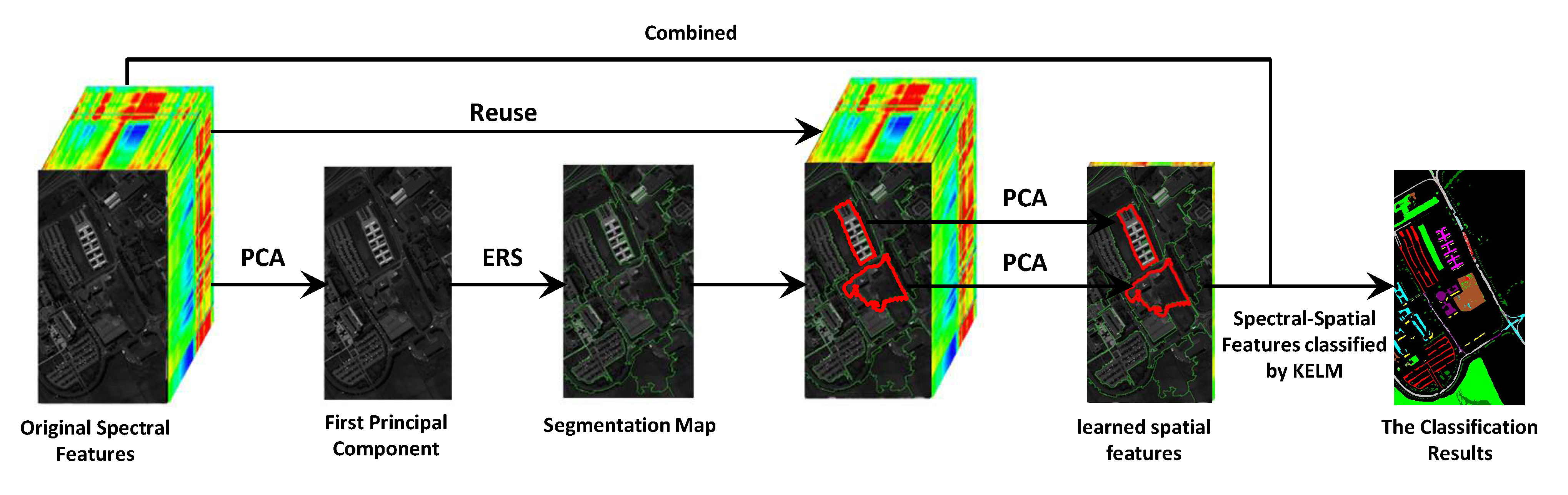
Being a simple yet effective preprocessing method, principal component analysis (PCA) [52] is one of the most widely used dimensionality reduction technique for the application of HSIs. PCA converts original possibly correlated variables into linearly uncorrelated variables (i.e., principal components) by using an orthogonal transformation. Given the input matrix $\mathbf{X}\in {\mathbb{R}}^{d\times N}$ with N input samples and d input features, PCA aims at finding a linear transformation relationship between the original d-dimensional space $\mathbf{X}$ and a low e-dimensional space ${\mathbf{X}}^{\prime }\in {\mathbb{R}}^{e\times N}$ by maximizing data variance in ${\mathbf{X}}^{\prime }$. Denote the transformation matrix as $\mathbf{W}\in {\mathbb{R}}^{d\times e}$, the linear transformation between $\mathbf{X}$ and ${\mathbf{X}}^{\prime }$ is represented as ${\mathbf{X}}^{\prime }={\mathbf{W}}^T\mathbf{X}$. An example of principal projection direction of PCA can be found in Figure 1a. Mathematically, the transformation matrix W can be determined by solving the following objective function,

$${\mathbf{W}}^{*}=\underset{{\mathbf{W}}^T\mathbf{W}=\mathbf{I}}{argmax}\mathrm{Tr}\left({\mathbf{W}}^T\mathrm{Cov}\left(\mathbf{X}\right)\mathbf{W}\right),$$

(2)

where $\mathrm{Cov}(·)$ measures the covariance matrix. Due to the effectiveness and efficiency, there are a variety of PCA variants proposed to address the dimensionality reduction problem for HSIs. In [53], a nonparametric mutual information (MI) measure is employed on the components obtained via PCA to form a new dimensionality reduction method (called MI-PCA) for HSI analysis. In [54], a fast iterative kernel principal component analysis (FIKPCA) centers on solving eigenvectors during iterative learning instead of performing eigen decomposition, which greatly reduces both the space and time complexities. In [55], a novel dimensionality reduction method via regression (DRR for short) is introduced to generalize PCA with curvilinear features, which falls into the family of invertible transforms. The above-mentioned approaches are typically proposed to overcome the limitations of PCA in HSI analysis. More detailed information of limitations of principal components analysis for HSI analysis can be found in the work of Prasad and Bruce [56].

2.3. Extreme Learning Machine

Extreme learning machine (ELM) is an emerging learning model for training “generalized” single hidden layer feedforward neural networks (SLFNs), which can achieve superior generalization performance with fast learning speed on complicated application problems [32,57]. ELM is composed of an input layer, a hidden layer and an output layer, where the input and hidden layers are connected by the input weights, while the output and hidden layers are connected by the output weights. The network structure of ELM is shown in Figure 1b. As opposed to conventional neural networks with iterative parameter tuning, ELM need not to iteratively adjust its network parameters. In general, the basic ELM is usually partitioned into two main steps: ELM feature mapping and ELM parameter solving [58]. In the first step, a latent representation is obtained from original input data via nonlinear feature mapping. According to ELM theory, various activation functions can be adopted in ELM feature mapping stage. Activation functions commonly used in the literature involve sigmoid function, Gaussian function, sine function, cosine function, etc. All activation functions adopted in ELM are infinitely differentiable [59]. In the second step, output weight parameters are then analytically solved by the Moore–Penrose (MP) generalized inverse and the minimum norm least-squares solution of a general linear system without any learning iteration. Given N distinct training samples, $\{\mathbf{X},\mathbf{Y}\}$ $={\left\{({\mathbf{x}}_i,{\mathbf{y}}_i)\right\}}_{i=1}^N$, where ${\mathbf{x}}_i\in {\mathbb{R}}^d$ is a d-dimensional input vector and ${\mathbf{y}}_i\in {\mathbb{R}}^c$ is a c-dimensional target vector. The ELM network with Q hidden nodes is represented as the following equation:

$${\mathbf{y}}_i=\sum _{j=1}^Q{\mathbf{\beta }}_j{h}_j({\mathbf{\varpi }}_j·{\mathbf{x}}_i+b_j),i=1,2,\dots ,N;$$

(3)

where ${\mathbf{\varpi }}_j\in {\mathbb{R}}^d$ is the input weight vector, $b_j$ is the hidden layer bias, and ${\mathbf{\beta }}_j\in {\mathbb{R}}^c$ is the output weight vector for the jth hidden node. $h_j(·)$ is the output value of the jth hidden node. For simplification, Equation (3) can be compactly represented as

$$\mathbf{H}\mathbf{\beta }=\mathbf{Y},$$

(4)

where $\mathbf{H}$ is the hidden layer output matrix and $\mathbf{\beta }$ is the output weight matrix.

Due to the remarkable advantages of ELM, numerous effective ELM variants are proposed to address the applications of remote sensing. The satisfactory performance of ELM on HSIs are supported by theoretical studies. In ELM theories, universal approximation capability [58] and classification capability [59] attract great attention and become research focuses. In [7], an ELM based method for HSI anlaysis is presented to automatically determine model parameters with the differential evolution (DE) optimization. In [60], a novel spatiotemporal fusion method using ELM is advocated to provide useful information in high resolution earth observation. In [61], two ensemble ELM methods with the idea of Bagging and AdaBoost are proposed to overcome the weakness of randomly generated parameters for HSI classfication. In [62], an advanced active learning ELM approach is presented as a query-by-Bagging algorithm, which selects the most informative pixels in a voting manner. In the literature, there are a good deal of ELM based methods to address the remote sensing application problems.

3. Proposed Spectral-Spatial Classification Model

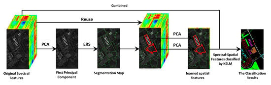
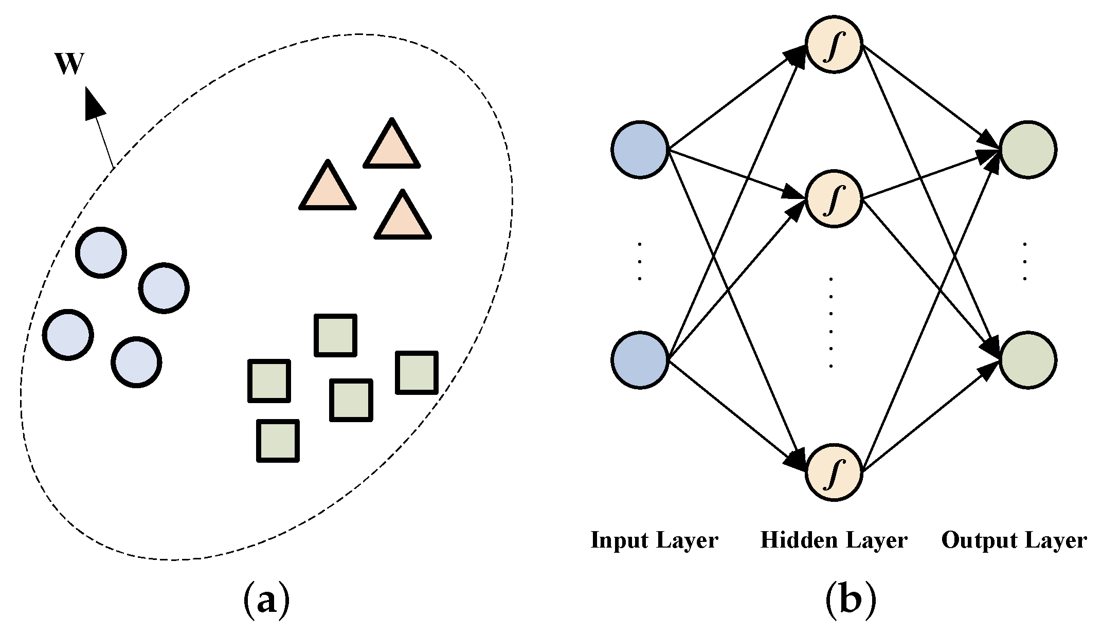
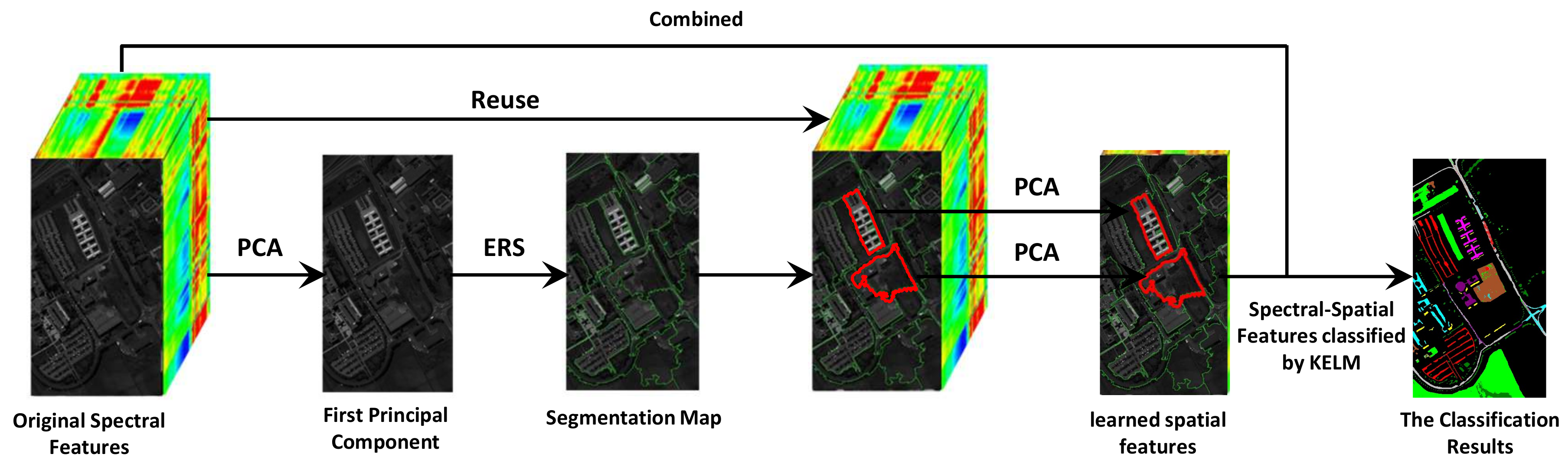
In this section, we elaborate the details of the proposed spectral-spatial classification model for HSI analysis. Figure 2 shows the schematic of the proposed model. The section begins by learning superpixel-based spatial features. The kernel based ELM used to be the classifier follows. Algorithm 1 presents the pseudocode of the proposed method.

Algorithm 1 Pseudocode. for SP-KELM

Input: HSI cube $\mathcal{X}$$\in {\mathbb{R}}^{M\times N\times L}$; Number of hidden nodes Q; Coefficient C; Number of superpixel segmentation $S_s$; Dimension of spatial features $S_f$;    Output: The predicted labels for each tesing pixel in HSI cube; 1: Reshape 3D HSI cube $\mathcal{X}$ to a 2D spectral matrix ${\mathbf{X}}^{spec}\in {\mathbb{R}}^{L\times P}$ $(P=MN)$; 2: Perform PCA on ${\mathbf{X}}^{spec}$ to obtain the first principal component $I_f$; 3: Perform ERS on $I_f$ to get the superpixel segmentation map and the segmented spectral matrices ${\mathbf{X}}^{spec}={\cup }_k^{S_s}{\mathbf{X}}_k^{spec}$; 4: Apply PCA on each segmented spectral matrice ${\mathbf{X}}_k^{spec}$ to obtain the reduced spatial features ${\mathbf{X}}_k^{spat}$ with the dimension of $S_f$; 5: Combine the reduced spatial features for HSI by ${\mathbf{X}}^{spat}={\cup }_k^{S_s}{\mathbf{X}}_k^{spat}$; 6: Combine ${\mathbf{X}}_k^{spec}$ and ${\mathbf{X}}^{spat}$ to get the spectral-spatial features ${\mathbf{X}}^{ss}=[{\mathbf{X}}^{spec};{\mathbf{X}}^{spat}]$ for HSI; 7: Apply the KELM on the spectral-spatial features ${\mathbf{X}}^{ss}$ by dividing it into the training and testing dataset; 8: Return the predicted labels for each testing pixel for HSI.

3.1. Superpixel Based Spatial Features

For HSIs, spatial features are learned from various perspectives in diverse studies. Dimensionality reduction approaches can be also employed to extract informative spatial features from HSIs. For example, in [63], a hierarchical PCA approach is presented to reduce the dimensionality of hyperspectral data, where an HSI is partitioned into different spatial domains (i.e., $2\times 2$ or $4\times 4$ parts of the image). The hierarchical PCA can exploit certain spatial information into the reduced feature space. However, the fixed size of each partitioned region cannot accurately reflect the spatial domains of HSIs. To effectively exploit the spatial information into the reduced feature space, in [29], the superpixel-based PCA approach is introduced for spatial feature extraction, which employs a superpixel segmentation method to obtain homogeneous regions instead of simply generating the same size of spatial regions. Motivated by this, we attempt to generate spatial features in this manner.

Superpixel segmentation approaches partition HSIs according to the intrinsic characteristics, which efficiently capture the spatial information. As in many superpixel segmentation-based approaches, ERS is adopted to generate homogeneous regions from HSIs for its efficiency and efficacy. Other effective and efficient superpixel segmentation method can be also employed to replace the ERS. Given an HSI cube $\mathcal{X}$ $\in {\mathbb{R}}^{M\times N\times L}$, M and N represent the length and width of an image and L denotes the number of sampled wavelengths. The 3D HSI cube can be reshaped to a 2D spectral matrix ${\mathbf{X}}^{spec}\in {\mathbb{R}}^{L\times P}$ $(P=MN)$, where a single column denotes one pixel in the HSI. Initially, the first principal component of the HSI, $I_f\in {\mathbb{R}}^P$ (i.e., $I_f\in {\mathbb{R}}^{M\times N}$), is obtained by PCA to capture the primary knowledge hidden in the image. This operator lessens the computational burden in the process of superpixel segmentation. During the superpixel segmentation process, we then perform ERS on the first principal component $I_f$ to generate superpixel segmentations,

$$I_f=\underset{k}{\overset{S_s}{\cup }}{\mathcal{H}}_k,s.t.{\mathcal{H}}_k\cap {\mathcal{H}}_g=⌀,(k\ne g),$$

(5)

where $\mathcal{H}$${}_k$ is the kth segmentation, and $S_s$ represents the number of segmentations.

By partitioning an HSI to superpixels, the abundant spatial information of land covers can be exploited. We then incorporate the spatial information into the reduced feature space with PCA. Specifically, according to the segmentation ${\left\{{\mathcal{H}}_k\right\}}_{k=1}^{S_s}$, the 2D HSI matrix is partitioned into multiple matrices ${\mathbf{X}}^{spec}={\cup }_k^{S_s}{\mathbf{X}}_k^{spec}$. PCA is then applied on the segmented matrices (i.e., superpixels) to obtain the reduced spatial features. These reduced spatial features can be combined to form a spatial HSI matrix, which is denoted as ${\mathbf{X}}^{spat}$. When the traditional PCA algorithm is applied on an entire image, the principal projection direction shows the uniqueness. For the superpixel based PCA method, it can find the intrinsic projection directions for all superpixel segmentations. Compared to the traditional PCA method, the superpixel based PCA method flexibly takes full advantage of the spatial information to extract spatial features.

3.2. Kernel Based Extreme Learning Machine

Kernel learning approaches are a type of machine learning algorithms to identify general relationships between features and labels. Compared to the general approaches, kernel learning methods do better in simulating the nonlinear relationships between features and labels. In general, nonlinear relationships between pixels and ground covers are prevalent in HSIs. Therefore, we adopt a kernel based ELM (KELM) method as the classifier in the proposed spectral-spatial classification model. The KELM method integrates kernel learning into ELM and extends the explicit activation function to an implicit mapping function, which avoids the randomly generated parameter issue and demonstrates the superior generalization capability. In diverse HSI learning models, KELM is widely used as the classifier to predict the ground covers for all pixels [13,34].

By combining the original spectral features ${\mathbf{X}}^{spec}$ and the learned spatial features ${\mathbf{X}}^{spat}$, we get the spectral-spatial features ${\mathbf{X}}^{ss}=[{\mathbf{X}}^{spec};{\mathbf{X}}^{spat}]$. To effectively solve Equation (4) for ELM, the output weight matrix can be calculated as

$$\mathbf{\beta }={\mathbf{H}}^{+}\mathbf{Y},$$

(6)

where ${\mathbf{H}}^{+}$ is the Moore–Penrose generalized inverse for $\mathbf{H}$. Actually, matrix ${\mathbf{H}}^{+}$ can be determined as ${\mathbf{H}}^{+}={\mathbf{H}}^T{\left(\mathbf{H}{\mathbf{H}}^T\right)}^{-1}$ [31], where ${\mathbf{H}}^T$ is the transpose of $\mathbf{H}$. To achieve better generalization, a positive value C is added to the diagonal elements of $\mathbf{H}{\mathbf{H}}^T$. Therefore, Equation (6) can be represented as $\mathbf{\beta }={\mathbf{H}}^T{(\frac{\mathbf{I}}{C}+\mathbf{H}{\mathbf{H}}^T)}^{-1}\mathbf{Y}$, which can achieve by the least squares estimation cost function to solve $\mathbf{\beta }$. Given input spectral-spatial data ${\mathit{x}}_i^{ss}$, the ELM classifier is then mathematically formulated as

$$f\left({\mathit{x}}_i^{ss}\right)=\mathbf{h}\left({\mathit{x}}_i^{ss}\right)\mathbf{\beta }=\mathbf{h}\left({\mathit{x}}_i^{ss}\right){\mathbf{H}}^T{\left(\frac{\mathbf{I}}{C}+\mathbf{H}{\mathbf{H}}^T\right)}^{-1}\mathbf{Y}.$$

(7)

In ELM, a feature mapping $\mathit{h}\left({\mathit{x}}_i^{ss}\right)$ is unknown to users. Therefore, we apply Mercer’s condition and define a kernel matrix for ELM as

$${\Omega }_{ELM}=\mathbf{H}{\mathbf{H}}^T,$$

(8)

where the ith row and rth column element is ${\Omega }_{EL{M}_{i,r}}=\mathit{h}\left({\mathit{x}}_i^{ss}\right)·\mathit{h}\left({\mathit{x}}_r^{ss}\right)=K({\mathit{x}}_i^{ss},{\mathit{x}}_r^{ss})$. For the ith row vector in ${\Omega }_{ELM}$, ${\Omega }_{EL{M}_i}=\mathit{h}\left({\mathit{x}}_i^{ss}\right){\mathbf{H}}^T=[K({\mathit{x}}_i^{ss},{\mathit{x}}_1^{ss});\cdots ;K({\mathit{x}}_i^{ss},{\mathit{x}}_N^{ss})]$. Thus, the formulation of KELM is denoted as

$$f\left({\mathit{x}}_i^{ss}\right)=\mathit{h}\left({\mathit{x}}_i^{ss}\right){\mathbf{H}}^T{\left(\frac{\mathbf{I}}{C}+\mathbf{H}{\mathbf{H}}^T\right)}^{-1}\mathbf{Y}={\left[\begin{array}{c}K({\mathit{x}}_i^{ss},{\mathit{x}}_1^{ss})\\ ⋮\\ K({\mathit{x}}_i^{ss},{\mathit{x}}_N^{ss})\end{array}\right]}^T{\left(\frac{\mathbf{I}}{C}+{\Omega }_{ELM}\right)}^{-1}\mathbf{Y}.$$

(9)

To further enhance the performance of the proposed spectral-spatial classification model, the cross-validation is used to determine suitable parameter C for KELM.

4. Experiments

We conducted experiments to verify the effectiveness and efficiency of the proposed SP-KELM method in hyperspectral image classification application.

4.1. Hyperspectral Datasets

To verify the performance of the proposed SP-KELM method, three publicly available HSI datasets (http://alweb.ehu.es/ccwintco/index.php?title=Hyperspectral_Remote_Sensing_Scenes), including Indian Pine, University of Pavia and Salinas Scene, were used in the experiments.

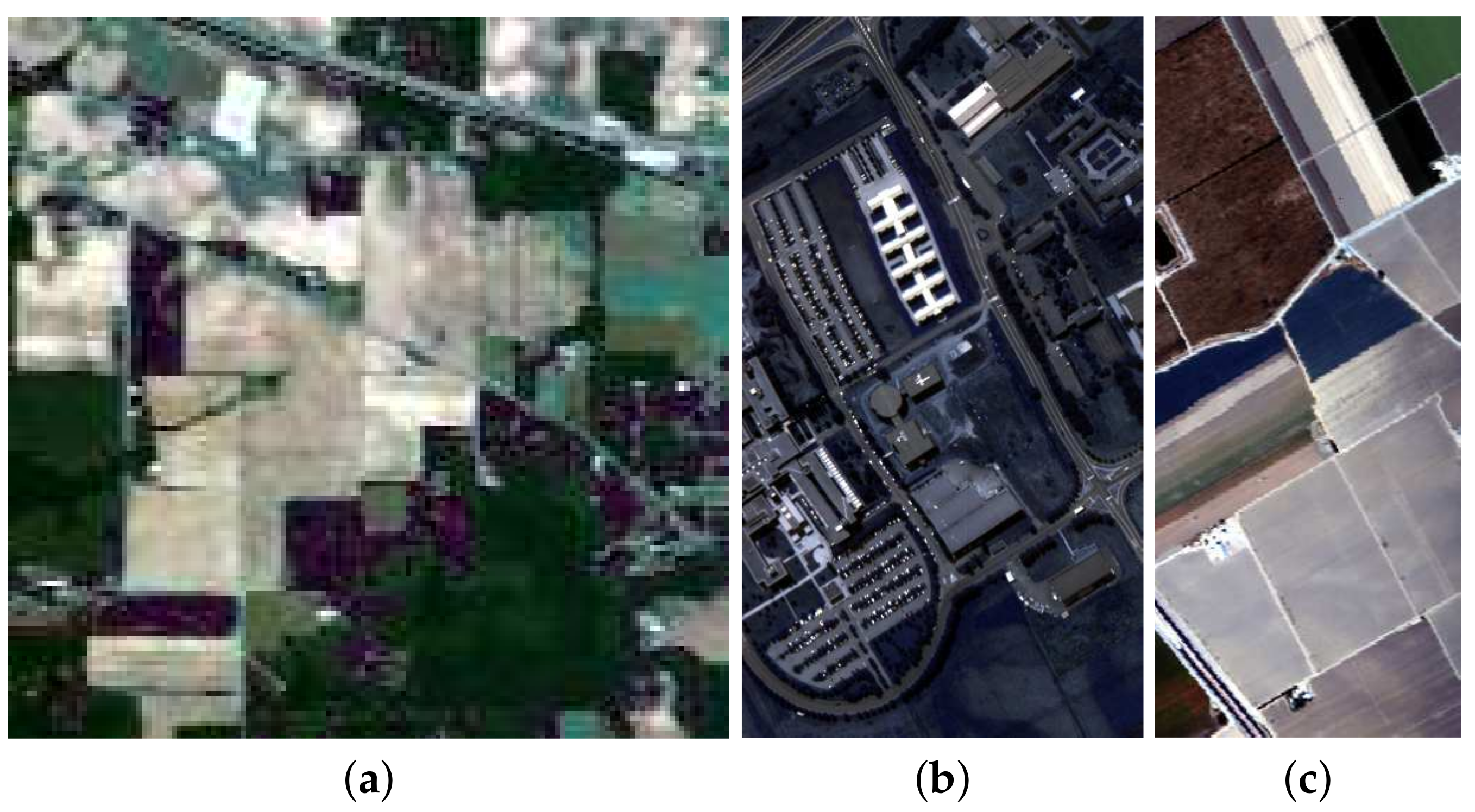
The Indian Pine dataset was captured by the Airborne Visible/Infrared Imaging Spectrometer (AVIRIS) sensor in 1992, and is a scene of Northwest Indiana. In this scene, there are $145\times 145$ pixels and 220 spectral bands with 20 m spatial resolution in the 0.4–2.45 m region. After removing 20 bands with low signal noise ratio, 200 bands were used for classification. The Indian Pine dataset records 16 different land covers of the agricultural fields with regular geometry. There are 10,249 labeled pixels contained in the ground-truth map, details of which are shown in

Table 1. Statistics of the hyperspectral image datasets.

Indian Pines		University of Pavia		Salinas Scene
Class Names	Numbers	Class Names	Numbers	Class Names	Numbers
1. Alfalfa	46	1. Asphalt	6631	1. Broccoli green weeds 1	2009
2. Corn-notill	1428	2. Bare soil	18,649	2. Broccoli green weeds 2	3726
3. Corn-mintill	830	3. Bitumen	2099	3. Fallow	1976
4. Corn	237	4. Bricks	3064	4. Fallow rough plow	1394
5. Grass-pasture	483	5. Gravel	1345	5. Fallow smooth	2678
6. Grass-trees	730	6. Meadows	5029	6. Stubble	3959
7. Grass-pasture-mowed	28	7. Metal sheets	1330	7. Celery	3579
8. Hay-windrowed	478	8. Shadows	3682	8. Grapes untrained	11,271
9. Oats	20	9. Trees	947	9. Soil vineyard develop	6203
10. Soybean-notill	972			10. Corn senesced green weeds	3278
11. Soybean-mintill	2455			11. Lettuce romaine 4 wk	1068
12. Soybean-clean	593			12. Lettuce romaine 5 wk	1927
13. Wheat	205			13. Lettuce romaine 6 wk	916
14. Woods	1265			14. Lettuce romaine 7 wk	1070
15. Buildings-Grass-Trees-Drives	286			15. Vineyard untrained	7268
16. Stone-Steel-Towers	93			16. Vineyard vertical trellis	1807
Total Number	10,249	Total Number	42,776	Total Number	54,129

. The false color composition of the Indian Pine data is shown in Figure 3a.

The University of Pavia dataset was collected by the Reflective Optics System Imaging Spectrometer (ROSIS-3) sensor in 2002, recording a scene from the University of Pavia, Italy. In this scene, there are $610\times 340$ pixels to present the spatial coverage, of which the spectral coverage is 0.43–0.86 $\mathsf{\mu }$m and the geometric resolution is 1.3 m. The scene contains 115 spectral bands, of which 12 noisy and uninformative bands were removed. There are 42,776 labeled pixels with 9 diverse land covers. For the University of Pavia data, the details of labeled pixels are represented in Table 1, and the false color composition is demonstrated in Figure 3b.

The Salinas Scene dataset was acquired by the AVIRIS sensor over Salinas Valley, California, USA in 1998. The scene contains $512\times 217$ pixels over 0.4–2.5 $\mathsf{\mu }$m with the geometric resolution of 3.7 m. It involves 204 spectral bands by removing 20 water absorption and atmospheric effects bands. There are 54,129 labeled pixels related to 16 different land covers in the documented dataset, the details of which are demonstrated in Table 1. The false color composition of the Salinas Scene data is represented in Figure 3c.

4.2. Competing Methods and Experimental Setting

In the experiments, we compared the proposed SP-KELM model with different competing methods. These compared methods can be divided into two parts: spectral approaches and spectral-spatial approaches. The spectral approaches are SVM [6], ELM [7] and KELM [12], which only use the spectral bands as input data. Another spectral approach used in the experiments is PCA-KELM, where the original spectral features and the low-dimensional spectral features extracted by the conventional PCA are combined to form a new feature space for the classification of KELM. The spectral-spatial approaches are KELM with composite kernels (CK-KELM) [12] and KELM with local binary patterns (LBP-KELM) [13]. Three widely used evaluation metrics, including overall accuracy (OA), average accuracy (AA) and kappa coefficient, were adopted to assess the testing classification performance of all compared methods on the three HSI datasets. The overall accuracy measures the percentage of correctly predicted testing pixels. The average accuracy averages the predicted classification accuracies of all pixels with different land covers. The kappa coefficient is a statistical measure to represent the degree of classification agreement. All experiments were performed on a computer with an Intel(R) Core(TM) 2.70 GHZ CPU and 8 GB RAM with Matlab R2016a. To avoid any bias, the presented experimental results were averaged from repeating the experiments 10 times.

The radial basis function (RBF) kernel parameter $\sigma$ and penalty parameter C involved in SVM were varied in the range of $\{2^{-4},2^{-3},\dots ,2^4\}$ and $\{2^{-6},2^{-4},\dots ,2^{12}\}$. In ELM, the sigmoid function was taken as the activation function and the number of hidden nodes defaulted to 1000 as in [12]. The parameter C ranged $\{2^{-6},2^{-4},\dots ,2^{12}\}$ and the input parameters in ELM were randomly selected from the uniform distribution of $[-1,1]$. For all methods related to KELM, the RBF kernel was adopted and the kernel parameter $\sigma$ ranged $\{2^{-4},2^{-3},\dots ,2^4\}$. Besides, parameter C was varied in $\{2^{-6},2^{-4},\dots ,2^{12}\}$. For PCA-KELM and SP-KELM, the dimension of the reduced spatial features was set as 30. In SP-KELM, the number of segmented superpixels defaulted as 100. The parameters in CK-KELM and LBP-KELM were tuned for specific HSI datasets. In the above methods, threefold cross-validation with a grid-search strategy was used to determine the optimal values for parameters $\sigma$ or C. Specifically, the original training set was divided into three equally-sized subsets at random. Two subsets were employed for model training and the remaining subset was utilized for validation. This process was repeated until each subset was consecutively used for validation. Finally, the parameters with the optimal performance were adopted for the subsequent testing process.

4.3. Experimental Comparison

We begin our discussion on comparison results between the proposed SP-KELM method and the competing methods. The discussions of the three HSI datasets are presented in the following descriptions.

(1) Experiments on the Indian Pine Dataset: For the Indian Pines dataset, the number of pixels with labeled land covers ranges from 20 to 2455. The classification on such unbalanced distribution dataset is a challenging problem. To study the performance of different algorithms on this challenging dataset, we randomly selected a fixed number of the labeled pixels from each land cover as training data. Specifically, 30 training pixels were arbitrarily chosen when the total number of the pixels for land covers was more than 60. Otherwise, half of the training pixels were selected at random. The remaining labeled pixels were employed for testing. By doing so, the unbalanced problem in exploring the Indian Pine data could be alleviated. The comparison results of the Indian Pines dataset are shown in

Table 2. Performance comparison of all compared methods on the Indian Pines dataset.

Class	#Samples		Spectral Approaches				Spectral-Spatial Approaches
	Train	Test	SVM	ELM	KELM	PCA-KELM	CK-KELM	LBP-KELM	SP-KELM
1	23	23	93.04	86.52	92.61	93.04	99.57	100.00	100.00
2	30	1398	52.63	45.89	56.09	54.59	85.94	83.63	89.11
3	30	800	62.99	39.05	60.40	60.16	89.11	93.51	92.42
4	30	207	77.05	63.62	78.84	80.19	99.37	99.52	95.56
5	30	453	87.99	83.91	87.81	85.87	90.49	97.68	97.09
6	30	700	91.19	92.27	91.76	91.97	99.34	99.40	98.30
7	14	14	88.57	90.71	91.43	90.71	100.00	100.00	97.14
8	30	448	93.24	83.39	94.33	92.28	99.78	99.98	99.64
9	10	10	82.00	66.00	95.00	87.00	100.00	100.00	100.00
10	30	942	63.54	57.01	64.10	63.66	87.98	84.58	89.82
11	30	2425	52.88	46.29	54.41	53.30	82.39	82.29	90.18
12	30	563	61.51	60.02	73.11	69.57	93.02	84.30	92.50
13	30	175	97.43	99.26	98.40	98.46	99.89	100.00	99.43
14	30	1235	85.96	80.08	85.21	80.13	93.45	99.70	98.95
15	30	356	57.39	57.78	66.07	62.53	99.47	98.79	98.82
16	30	63	95.87	91.90	91.90	92.70	99.84	100.00	99.05
OA (%)			67.46	60.62	69.19	67.53	89.84	90.14	93.43
AA (%)			77.70	71.48	80.09	78.51	94.98	95.21	96.13
Kappa			0.6335	0.5576	0.6531	0.6353	0.8844	0.8878	0.9250

.

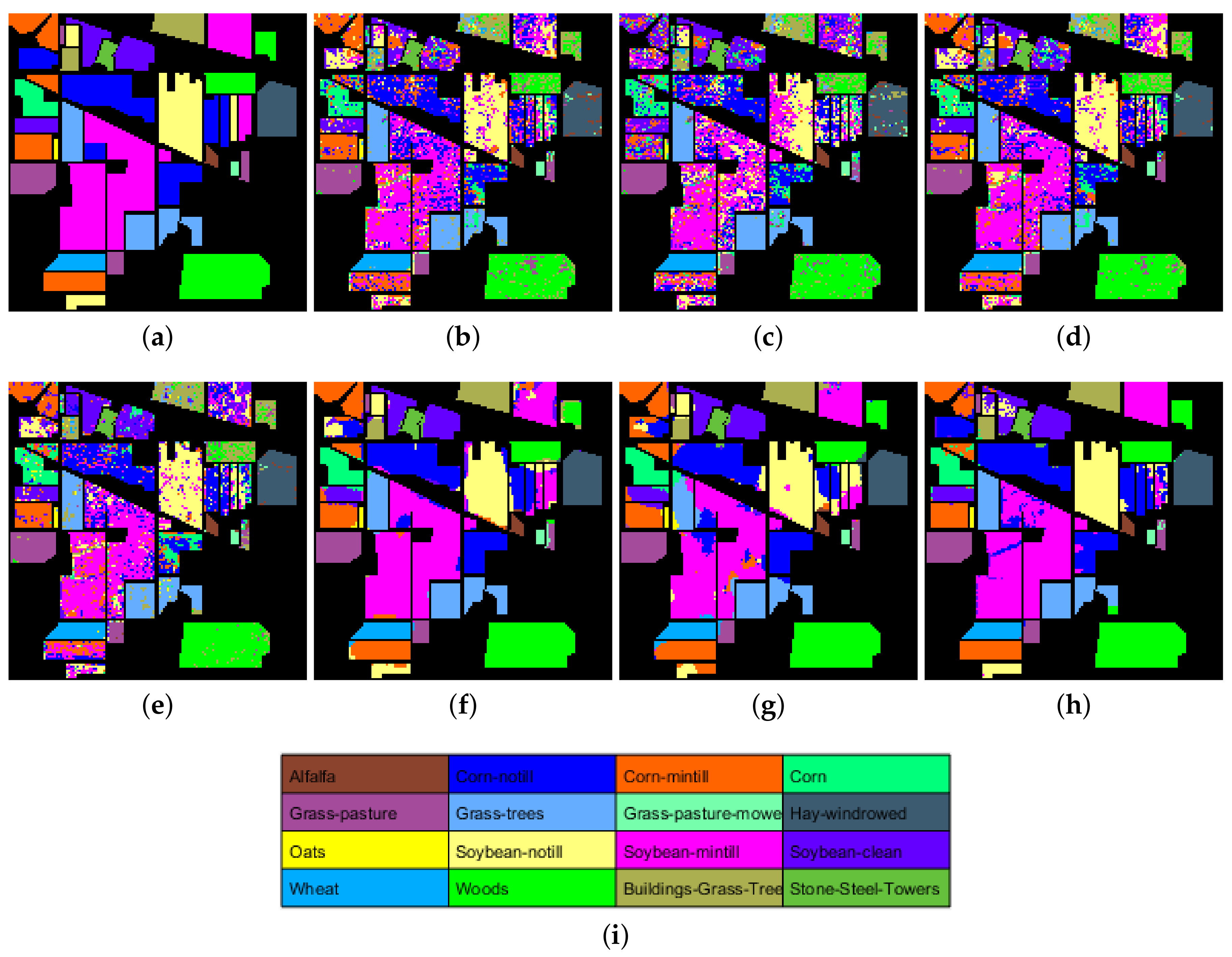
In Table 2, among the spectral approaches, ELM demonstrates the worst results especially for some specific land covers (e.g., corn-mintill and oats) for the absence of the kernel, which is more capable of exploring the nonlinear relationship between features and land covers. The land covers of corn-mintill and oats are very close to other similar land covers, which may result in difficulty of identifying these land covers. Compared to KELM, PCA-KELM cannot extract additional informative spectral features to improve the classification performance of the Indian Pine data. This is because the conventional PCA cannot always extract discriminative features from original data. When introducing extra spatial features, the performance of HSI approaches can be dramatically improved. This can be found from the experimental results of the spectral-spatial approaches in Table 2. For the spectral-spatial approaches, they adopt different manners to extract spatial features from spectral features. CK-KELM generates spatial features based on the spatial neighboring pixels of a general pixel, while LBP-KELM adopts local binary pattern to exploit texture information into spatial features. According to the results in Table 2, SP-KELM shows its superiority to CK-KELM and LBP-KELM. It demonstrates that SP-KELM can extract more discriminative spatial features than the other two spectral-spatial approaches. The classification maps of all compared approaches on the Indian Pines dataset are depicted in Figure 4, where overall accuracies of different compared methods are in accordance with our observation. More detailed experimental results can be found in Table 2 and Figure 4.

(2) Experiments on the University of Pavia Dataset: For comparison purpose, 30 pixels from each land cover were randomly chosen to form training data, and the remaining pixels were all regarded as testing data. For the University of Pavia dataset, the comparison results are represented in

Table 3. Performance comparison of all compared methods on the University of Pavia dataset.

Class	#Samples		Spectral Approaches				Spectral-Spatial Approaches
	Train	Test	SVM	ELM	KELM	PCA-KELM	CK-KELM	LBP-KELM	SP-KELM
1	30	6601	69.47	37.37	62.56	68.94	83.83	81.39	83.29
2	30	18,619	72.76	71.24	71.67	76.07	93.31	86.43	90.12
3	30	2069	69.68	91.00	79.42	78.62	85.05	91.47	98.66
4	30	3034	93.19	94.11	92.99	93.88	95.85	97.25	92.27
5	30	1315	99.04	99.95	99.26	99.48	99.97	99.79	99.58
6	30	4999	69.21	64.50	71.59	76.02	93.35	96.03	94.11
7	30	1300	88.94	91.35	91.12	93.68	97.66	99.96	98.58
8	30	3652	78.00	26.69	67.90	77.95	86.69	98.41	99.00
9	30	917	98.66	90.84	96.04	99.81	90.46	99.95	93.82
OA (%)			75.46	65.88	73.79	78.29	91.33	89.94	91.49
AA (%)			82.11	74.12	81.40	84.94	91.80	94.52	94.38
Kappa			0.6879	0.5719	0.6685	0.7234	0.8865	0.8704	0.8892

, and the classification maps of the competing methods are given in Figure 5.

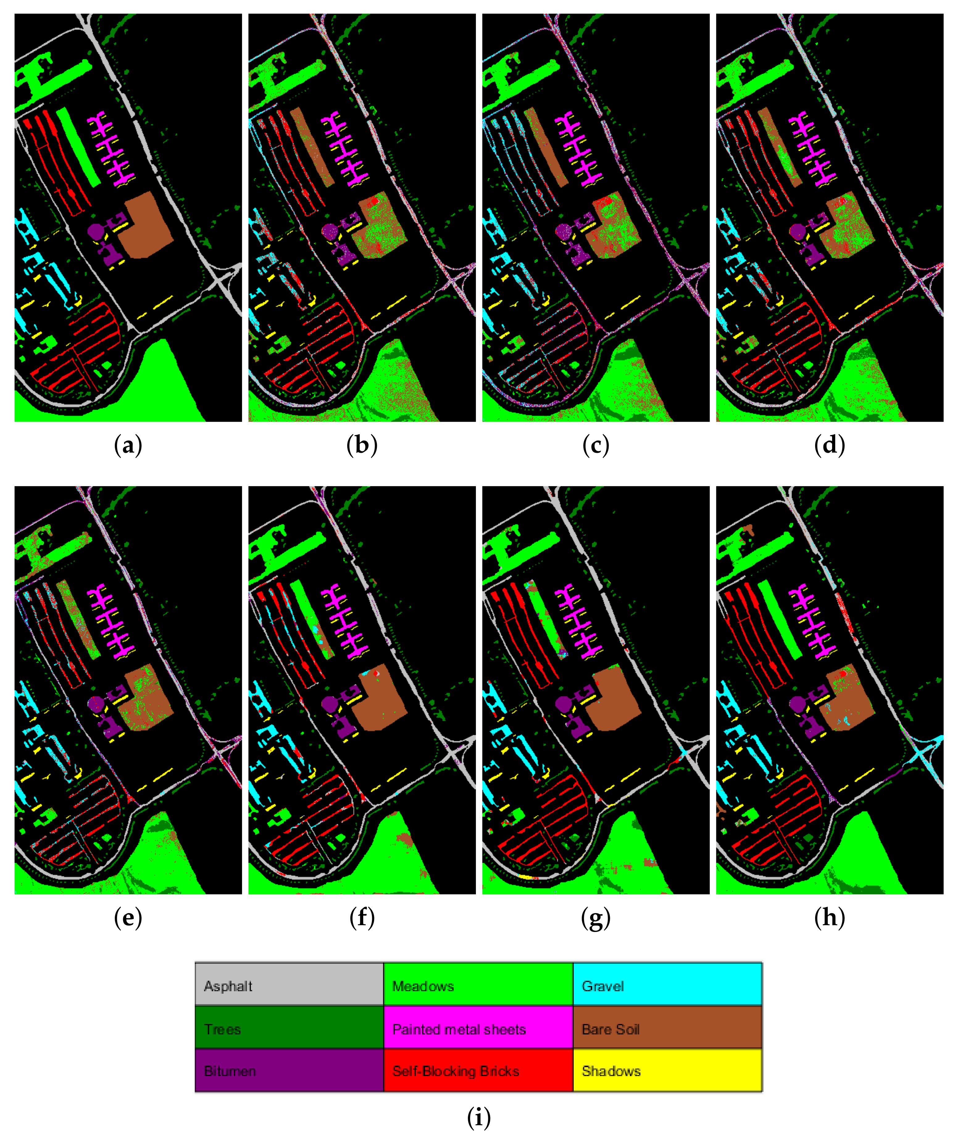
From the classification maps, we can find that the spectral approaches (e.g., SVM, ELM, KELM and PCA-KELM) exhibit lower classification accuracy than the spectral-spatial approaches (e.g., CK-KELM, LBP-KELM and SP-KELM), which is attributed to the missing spatial features. According to Table 3, ELM and PCA-KELM demonstrate the worst and best performance among the spectral approaches, respectively. Compared to ELM and PCA-KELM, the improvement of SP-KELM is high, at 38.8% and 16.8% for overall accuracy, 27.3% and 11.1% for average accuracy, and 55.4% and 22.9% for Kappa coefficient. Compared to KELM, PCA-KELM can learn informative spectral features with better classification performance from the University of Pavia data. For spectral-spatial approaches, CK-KELM and LBP-KELM show comparative classification performance compared to SP-KELM. For CK-KELM and LBP-KELM, the overall accuracy is 91.33% and 89.94%, the average accuracy is 91.80% and 94.52%, and the kappa coefficient is 0.8865 and 0.8704, respectively, which is slightly inferior to SP-KELM. The limited improvement of SP-KELM over CK-KELM and LBP-KELM is mainly due to two potential reasons. The land covers on the University of Pavia dataset mostly distribute with dispersiveness and constitute different special geometrical shapes. It is very hard to capture the useful spatial knowledge on such a complicated dataset. Besides, superpixel segmentation algorithms cannot commendably partition superpixels in accordance with the intrinsic texture information of such a dataset. Therefore, SP-KELM can only acquire slightly superior classification results than other methods. In summary, compared with spectral approaches, it is obvious that spectral-spatial approaches always achieve better classification performance because of introducing the underlying spatial information of the University of Pavia data.

(3) Experiments on the Salinas Scene Dataset: To evaluate the performance of all baselines, we randomly picked 30 pixels from each land cover to form training data, and the remaining pixels were used as testing data. For the Salinas Scene dataset, the comparison results are recorded in

Table 4. Performance comparison of all compared methods on the Salinas Scene dataset.

Class	#Samples		Spectral Approaches				Spectral-Spatial Approaches
	Train	Test	SVM	ELM	KELM	PCA-KELM	CK-KELM	LBP-KELM	SP-KELM
1	30	1979	98.71	99.68	99.52	99.69	99.45	100.00	100.00
2	30	3696	98.70	99.31	99.46	99.72	99.77	99.82	99.98
3	30	1946	94.29	91.96	92.02	99.18	98.75	99.92	99.67
4	30	1364	99.52	98.93	99.00	99.13	98.64	97.55	99.59
5	30	2648	96.36	98.65	97.67	97.16	99.23	98.49	99.24
6	30	3929	99.47	99.87	99.39	99.34	99.53	99.47	98.47
7	30	3549	99.33	99.43	99.49	99.39	98.14	99.83	98.11
8	30	11,241	67.03	75.70	75.68	73.27	84.93	89.25	94.70
9	30	6173	95.59	99.70	98.67	99.07	99.73	99.36	97.28
10	30	3248	91.74	90.90	92.76	92.16	96.15	98.24	97.67
11	30	1038	97.62	95.75	96.52	95.33	99.93	99.11	98.06
12	30	1897	99.86	83.11	99.98	100.00	99.98	97.64	97.75
13	30	886	98.01	97.96	97.98	97.78	99.50	96.65	98.21
14	30	1040	95.61	94.79	97.13	95.88	98.22	98.90	97.94
15	30	7238	72.67	56.44	68.19	71.18	84.10	86.97	99.43
16	30	1777	97.02	97.84	97.60	96.81	97.41	99.82	99.33
OA (%)			87.51	87.07	89.22	89.30	93.99	95.42	97.85
AA (%)			93.84	92.50	94.44	94.69	97.09	97.56	98.46
Kappa			0.8613	0.8559	0.8801	0.8811	0.9331	0.9490	0.9761

, and the classification maps of all baseline methods are demonstrated in Figure 6.

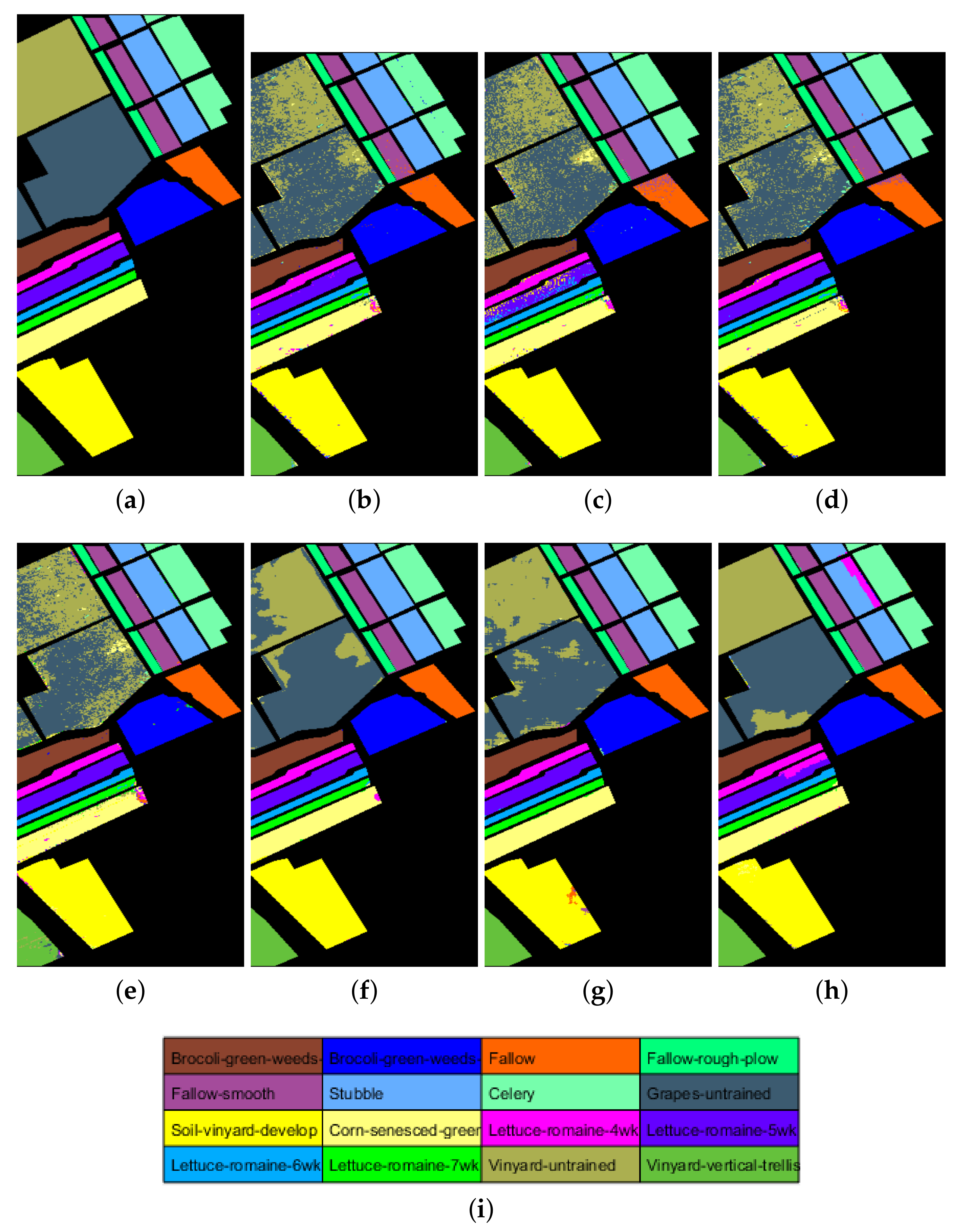
Similar to the Indian Pine dataset, the Salinas Scene dataset has the relatively regular spatial coverage for land covers. From the classification maps in Figure 6, among the spectral-spatial approaches, SP-KELM exhibits higher classification accuracy than CK-KELM and LBP-KELM for the effective spatial feature extraction. For spectral approaches, KELM and PCA-KELM demonstrate comparative performance and outperform SVM and ELM, which reveals the superiority of KELM. As shown in Table 4, we can observe that spectral-spatial approaches all gain better classification performance than spectral approaches. In details, for spectral approaches, SVM exhibits lower accuracy (67.03%) for the class of grapes untrained, and ELM achieves inferior accuracy (56.44%) for the class of vineyard untrained. For spectral-spatial approaches, they can obtain superior classification performance on all land covers. The overall accuracy of SP-KELM on the Salinas Scene dataset is 97.85%. Compared to CK-KELM and LBP-KELM, the enhancement of SP-KELM is more than 4.1% and 2.5%, respectively. Similar improvements for average accuracy and kappa coefficient can also be found in Table 4. Therefore, we can conclude that SP-KELM can learn more informative spatial features to boost the classification performance of the Salinas Scene dataset.

To further investigate the performance of the SP-KELM method for HSI analysis, we conducted experiments with different numbers of training pixels from each land cover. The overall accuracies for the experiments are represented in

Table 5. Overall accuracies of all baselines with different numbers of training pixels.

Dataset	T.P.s/L.C	Spectral Approaches				Spectral-Spatial Approaches
		SVM	ELM	KELM	PCA-KELM	CK-KELM	LBP-KELM	SP-KELM
Indian Pines	10	54.38	46.71	55.24	54.73	77.62	74.85	78.84
	15	59.76	52.13	62.32	60.20	84.56	81.73	87.18
	20	63.00	54.45	64.81	63.11	86.15	86.09	90.53
	25	65.13	58.81	66.87	65.93	88.16	88.41	91.97
	30	67.46	60.62	69.19	67.53	89.84	90.14	93.43
University of Pavia	10	64.38	61.53	66.06	71.79	77.02	72.24	80.26
	15	66.71	63.45	68.46	74.37	81.71	79.39	84.94
	20	70.34	63.27	70.34	76.98	88.16	87.54	88.21
	25	75.16	63.33	72.34	78.48	88.83	88.66	89.99
	30	75.46	65.88	73.79	78.29	91.33	89.94	91.49
Salinas Scene	10	84.33	84.78	85.82	85.62	90.73	89.29	88.58
	15	85.56	86.04	87.96	86.75	92.32	91.56	92.81
	20	86.34	85.85	87.35	87.14	92.79	93.67	95.90
	25	87.97	87.56	89.23	89.30	93.81	94.66	97.49
	30	87.51	87.07	89.22	89.30	93.99	95.42	97.61

. We successively selected $\{10,15,20,25,30\}$ pixels from each land cover at random to form training data, and the remaining pixels for testing. For simplification, the number of training pixels for each land cover is denoted as “T.P.s/L.C” in the table. With the increasing number of training pixels, the overall accuracies of all compared method become much better. This can be explained as these HSI classification methods benefit more discriminative information from the increase of labeled training pixels. From the results in Table 5, SP-KELM exhibits better performance than the other methods in most cases. Among the spectral approaches, ELM still exhibits the worst performance on all HSI datasets. By introducing the kernel learning, SVM and KELM show superior performance to ELM, as they are more capable of simulating the nonlinear relationships between features and land covers of HSI data. By introducing spatial information, spectral-spatial approaches are all superior to spectral approaches. The conventional PCA in PCA-KELM performs dimension reduction on the whole HSI, which can extract discriminative features from the original data. However, the spatial information hidden in HSIs cannot be extracted by means of such operation. By simultaneously using ERS and PCA on HSI, the spatial information is introduced into SP-KELM. This is the major difference between the PCA in PCA-KELM and the one in the proposed SP-KELM, which can achieve different algorithmic performance. For spectral-spatial approaches, with small size of training pixels on the Salinas Scene datasets, CK-KELM and LBP-KELM achieve better results, while SP-KELM demonstrates inferior performance. On the contrary, SP-KELM gains better results than CK-KELM and LBP-KELM with large sizes of training pixels on the Salinas Scene dataset. For the Indian Pines and University of Pavia datasets, SP-KELM always outperforms other two spectral-spatial approaches. According to the results in Table 5 and

Table 6. Dimension of spatial features learned by the spectral-spatial approaches on HSI datasets.

Dataset	CK-KELM	LBP-KELM	SP-KELM
Indian Pines	200	1770	30
University of Pavia	103	1770	30
Salinas Scene	204	1770	30

, SP-KELM shows its superiority to CK-KELM and LBP-KELM with fewer dimensions of the learned spatial features. Specifically, the dimensions of spatial features learned by SP-KELM and LBP-KELM are 30 and 1770 on all HSI datasets. For CK-KELM, the dimension of the learned spatial features is the size of the spectral features for the three HSI datasets (i.e., 200, 103 and 204, respectively). Therefore, we can conclude that SP-KELM is better than others in most instances. The superiority of SP-KELM is mainly attributed to the informative spatial features learned by superpixel-wise PCA.

4.4. Investigation on the Number of Superpixels

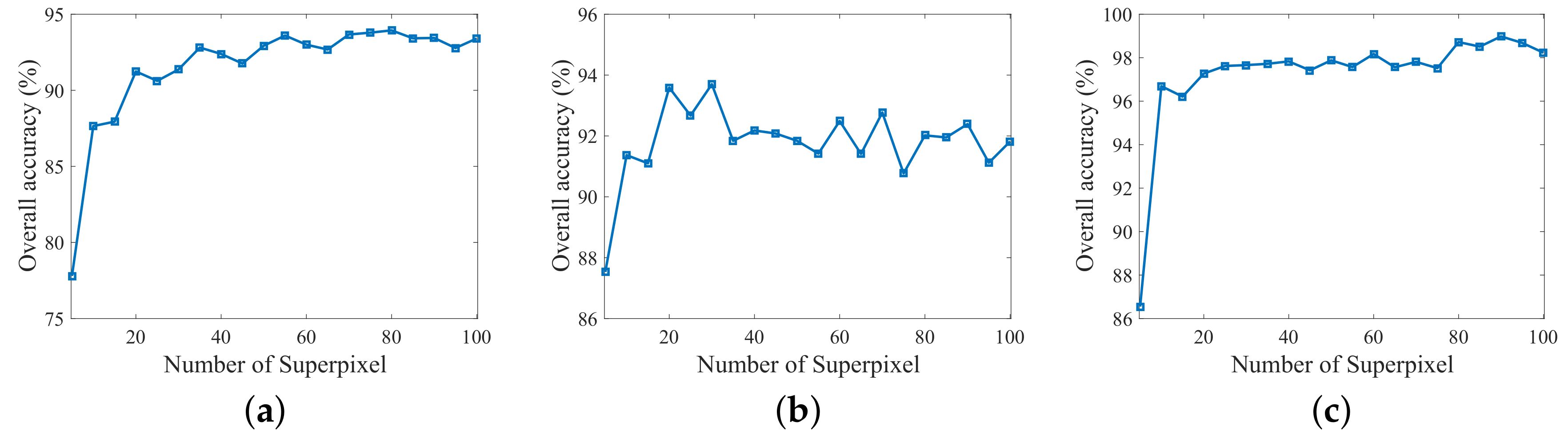
In SP-KELM, superpixels are segmented for PCA to extract superpixel-specific spatial features. The number of superpixel segmentations is unchangeable during the learning process. However, it is very difficult to identify suitable number of superpixel segmentations for HSIs. Therefore, we conducted an experimental to investigate the influence of different numbers of superpixels segmented from HSIs. For the three HSI datasets, the number of superpixels was varied in $\{5,100\}$ in units of 5. Experimental results with different numbers of superpixels are demonstrated in Figure 7.

For the Indian Pines and Salinas Scene datasets, pixels with the same land cover are spatially distributed together, which can be generally regarded as regular geometrical shapes. Therefore, the overall accuracies with different number of superpixels on these two HSI datasets are similar, which are shown in Figure 7a,c. Specifically, with the increase of superpixel number, the performance of SP-KELM first tends to increase and then keeps stable or even degrades. The highest overall accuracy is 93.94% for the Indian Pines dataset, where the optimal number of superpixel segmentations is 80. For the Salinas Scene dataset, the highest overall accuracy with 30 superpixel segmentations is 93.70%. Compared to the worst performance with a small number of superpixels, the improvement of SP-KELM with the optimal number of superpixels is 20.7% and 14.4% for the Indian Pines and Salinas Scene datasets, respectively. Different from the agricultural landscape in the above two HSI datasets, the University of Pavia dataset shows the city landscape to accord with the city function, which exhibits the unique spatial distribution for land covers. The overall accuracies with different numbers of superpixels on the University of Pavia dataset are shown in Figure 7b. There is no need to partition too many superpixel segmentations for the University of Pavia dataset. When the number of superpixels is set to 30, the optimal overall accuracy of SP-KELM can be achieved. According to the above experimental results, we can find that the optimal numbers of superpixels for different HSI datasets are not equal. This is because setting the optimal number of superpixels for a specific dataset mainly relies on the unique data characteristic. It is very hard to determine the optimal number of superpixels for different HSI datasets without any priori knowledge. Therefore, we can determine suitable numbers of superpixel segmentations according to the experiments.

4.5. Investigation on the Dimension of Superpixel Patterns

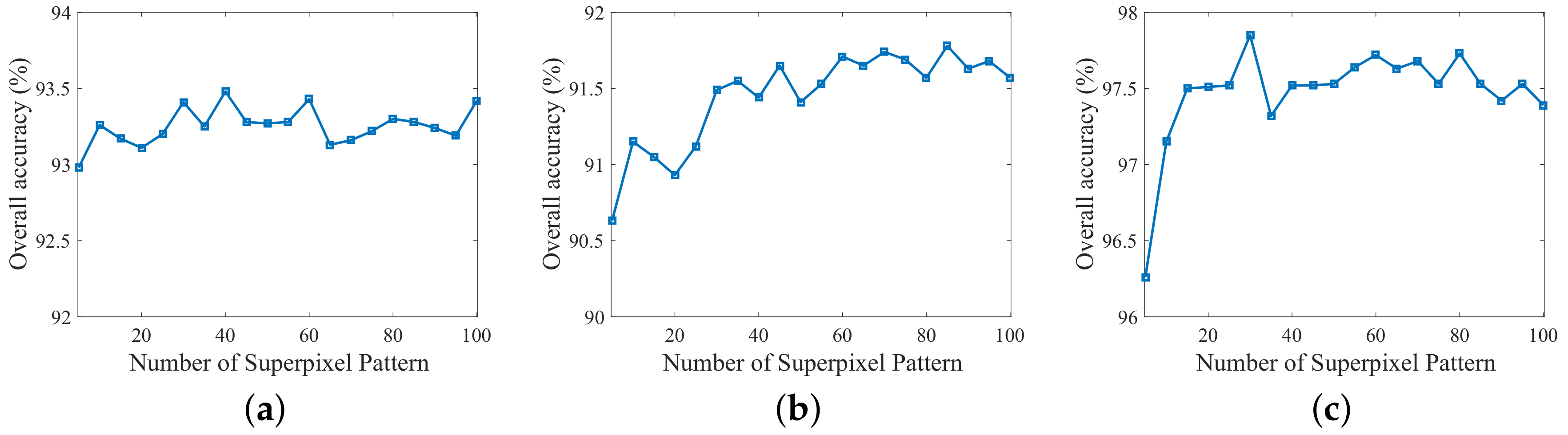
For the spectral-spatial HSI classification, the dimension of spatial features (i.e., superpixel patterns) in SP-KELM is a parameter that needs to be determined in advance. This is also a data-specific problem, where the parameter setting relies on the characteristic of dataset. To investigate the influence of different dimensions of spatial features, we report the experimental results in Figure 8. For the three HSI datasets, the dimension of spatial features ranges $\{5,10,15,20,\dots ,100\}$.

According to Figure 8a, the lowest and highest overall accuracies of SP-KELM are 92.98% and 93.48% for the Indian Pines dataset, which are obtained by setting 5 and 40 for the dimension of spatial patterns, respectively. For the University of Pavia dataset, the worst overall accuracy with five-dimensional spatial features is 90.63%, and the best one with 85-dimensional spatial features is 91.78%, which can be found in Figure 8b. For the Salinas Scene dataset in Figure 8c, when setting the dimension of spatial features as 5 and 30, the worst and best overall accuracies are 96.26% and 97.85%, respectively. It is clear that the difference between the worst and best performance of SP-KELM on the three HSI datasets is less than 2%. This means that the setting for the dimension of spatial features slightly influences the performance of SP-KELM in HSI analysis. Besides, according to the experimental results in Figure 8, setting the dimension of spatial features as 30 for the three HSI datasets as in the previous experiments is an advisable and acceptable choice.

5. Conclusions

In this paper, we propose a new spectral-spatial HSI classification model with superpixel pattern (SP) and kernel based extreme learning machine (KELM), called SP-KELM. In SP-KELM, superpixels are partitioned by the entropy rate segmentation (ERS) algorithm. The principal component analysis (PCA) method is then applied on these superpixels to extract superpixel-specific reduced features. The spatial features are obtained by combining superpixel-specific reduced features, which consists of the rich spatial information. By using both the original spectral features and extracted spatial features, KELM is adopted to perform the classification task for HSI datasets, which can greatly improve the classification performance. Experiments and comparisons on three HSI datasets confirmed the attractive properties of the proposed SP-KELM model compared to some baseline methods, which demonstrated that the potential spatial information benefits the HSI classification tasks. For future works, we will introduce various promising spectral-spatial HSI classification models to exploit the spatial information from different perspectives.

References

- Zhang, L.; Zhang, L.; Du, B. Deep learning for remote sensing data: A technical tutorial on the state of the art. IEEE Geosci. Remote Sens. Mag. 2016, 4, 22–40. [Google Scholar] [CrossRef]
- Ma, J.; Jiang, J.; Zhou, H.; Zhao, J.; Guo, X. Guided locality preserving feature matching for remote sensing image registration. IEEE Trans. Geosci. Remote Sens. 2018, 56, 4435–4447. [Google Scholar] [CrossRef]
- Ma, J.; Zhao, J.; Jiang, J.; Zhou, H.; Guo, X. Locality preserving matching. Int. J. Comput. Vis. 2019, 127, 512–531. [Google Scholar] [CrossRef]
- Jiang, J.; Chen, C.; Yu, Y.; Jiang, X.; Ma, J. Spatial-aware collaborative representation for hyperspectral remote sensing image classification. IEEE Geosci. Remote Sens. Lett. 2017, 14, 404–408. [Google Scholar] [CrossRef]
- Jiang, X.; Song, X.; Zhang, Y.; Jiang, J.; Gao, J.; Cai, Z. Laplacian Regularized Spatial-Aware Collaborative Graph for Discriminant Analysis of Hyperspectral Imagery. Remote Sens. 2019, 11, 29. [Google Scholar] [CrossRef]
- Melgani, F.; Bruzzone, L. Classification of hyperspectral remote sensing images with support vector machines. IEEE Trans. Geosci. Remote Sens. 2004, 42, 1778–1790. [Google Scholar] [CrossRef] [Green Version]
- Bazi, Y.; Alajlan, N.; Melgani, F.; Hichri, H.; Malek, S.; Yager, R.R. Differential evolution extreme learning machine for the classification of hyperspectral images. IEEE Geosci. Remote Sens. Lett. 2014, 11, 1066–1070. [Google Scholar] [CrossRef]
- Fauvel, M.; Tarabalka, Y.; Benediktsson, J.A.; Chanussot, J.; Tilton, J.C. Advances in spectral-spatial classification of hyperspectral images. Proc. IEEE 2013, 101, 652–675. [Google Scholar] [CrossRef]
- Fan, H.; Chang, L.; Guo, Y.; Kuang, G.; Ma, J. Spatial-Spectral Total Variation Regularized Low-Rank Tensor Decomposition for Hyperspectral Image Denoising. IEEE Trans. Geosci. Remote Sens. 2018, 56, 6196–6213. [Google Scholar] [CrossRef]
- Liu, T.; Gu, Y.; Jia, X.; Benediktsson, J.A.; Chanussot, J. Class-specific sparse multiple kernel learning for spectral–spatial hyperspectral image classification. IEEE Trans. Geosci. Remote Sens. 2016, 54, 7351–7365. [Google Scholar] [CrossRef]
- Camps-Valls, G.; Gomez-Chova, L.; Muñoz-Marí, J.; Vila-Francés, J.; Calpe-Maravilla, J. Composite kernels for hyperspectral image classification. IEEE Geosci. Remote Sens. Lett. 2006, 3, 93–97. [Google Scholar] [CrossRef]
- Zhou, Y.; Peng, J.; Chen, C.P. Extreme learning machine with composite kernels for hyperspectral image classification. IEEE J. Sel. Top. Appl. Earth Obs. Remote Sens. 2015, 8, 2351–2360. [Google Scholar] [CrossRef]
- Li, W.; Chen, C.; Su, H.; Du, Q. Local Binary Patterns and Extreme Learning Machine for Hyperspectral Imagery Classification. IEEE Trans. Geosci. Remote Sens. 2015, 53, 3681–3693. [Google Scholar] [CrossRef]
- Jain, A.K.; Ratha, N.K.; Lakshmanan, S. Object detection using Gabor filters. Pattern Recognit. 1997, 30, 295–309. [Google Scholar] [CrossRef]
- Chen, C.; Li, W.; Tramel, E.W.; Cui, M.; Prasad, S.; Fowler, J.E. Spectral-spatial preprocessing using multihypothesis prediction for noise-robust hyperspectral image classification. IEEE J. Sel. Top. Appl. Earth Obs. Remote Sens. 2014, 7, 1047–1059. [Google Scholar] [CrossRef]
- Chen, C.; Li, W.; Su, H.; Liu, K. Spectral-spatial classification of hyperspectral image based on kernel extreme learning machine. Remote Sens. 2014, 6, 5795–5814. [Google Scholar] [CrossRef]
- Tarabalka, Y.; Fauvel, M.; Chanussot, J.; Benediktsson, J.A. SVM and MRF-based method for accurate classification of hyperspectral images. IEEE Geosci. Remote Sens. Lett. 2010, 7, 736–740. [Google Scholar] [CrossRef]
- Li, W.; Prasad, S.; Fowler, J.E. Hyperspectral image classification using Gaussian mixture models and Markov random fields. IEEE Geosci. Remote Sens. Lett. 2014, 11, 153–157. [Google Scholar] [CrossRef]
- Li, J.; Bioucas-Dias, J.M.; Plaza, A. Spectral-spatial hyperspectral image segmentation using subspace multinomial logistic regression and Markov random fields. IEEE Trans. Geosci. Remote Sens. 2012, 50, 809–823. [Google Scholar] [CrossRef]
- Li, S.; Lu, T.; Fang, L.; Jia, X.; Benediktsson, J.A. Probabilistic fusion of pixel-level and superpixel-level hyperspectral image classification. IEEE Trans. Geosci. Remote Sens. 2016, 54, 7416–7430. [Google Scholar] [CrossRef]
- Priya, T.; Prasad, S.; Wu, H. Superpixels for Spatially Reinforced Bayesian Classification of Hyperspectral Images. IEEE Geosci. Remote Sens. Lett. 2015, 12, 1071–1075. [Google Scholar] [CrossRef]
- Roscher, R.; Waske, B. Superpixel-based classification of hyperspectral data using sparse representation and conditional random fields. In Proceedings of the 2014 IEEE International Geoscience and Remote Sensing Symposium (IGARSS), Quebec City, QC, Canada, 13–18 July 2014; pp. 3674–3677. [Google Scholar]
- Zhan, T.; Sun, L.; Xu, Y.; Yang, G.; Zhang, Y.; Wu, Z. Hyperspectral Classification via Superpixel Kernel Learning-Based Low Rank Representation. Remote Sens. 2018, 10, 1639. [Google Scholar] [CrossRef]
- Sun, H.; Ren, J.; Zhao, H.; Zabalza, J.; Marshall, S. Superpixel based Feature Specific Sparse Representation for Spectral-Spatial Classification of Hyperspectral Images. Remote Sens. 2019, 11, 536. [Google Scholar] [CrossRef]
- Fang, L.; Li, S.; Duan, W.; Ren, J.; Benediktsson, J.A. Classification of hyperspectral images by exploiting spectral-spatial information of superpixel via multiple kernels. IEEE Trans. Geosci. Remote Sens. 2015, 53, 6663–6674. [Google Scholar] [CrossRef]
- Fang, L.; Li, S.; Kang, X.; Benediktsson, J.A. Spectral-spatial classification of hyperspectral images with a superpixel-based discriminative sparse model. IEEE Trans. Geosci. Remote Sens. 2015, 53, 4186–4201. [Google Scholar] [CrossRef]
- Li, S.; Jia, X.; Zhang, B. Superpixel-based Markov random field for classification of hyperspectral images. In Proceedings of the 2013 IEEE International Geoscience and Remote Sensing Symposium (IGARSS), Melbourne, VIC, Australia, 21–26 July 2013; pp. 3491–3494. [Google Scholar]
- Zhang, S.; Li, S.; Fu, W.; Fang, L. Multiscale superpixel-based sparse representation for hyperspectral image classification. Remote Sens. 2017, 9, 139. [Google Scholar] [CrossRef]
- Jiang, J.; Ma, J.; Chen, C.; Wang, Z.; Cai, Z.; Wang, L. SuperPCA: A superpixelwise PCA approach for unsupervised feature extraction of hyperspectral imagery. IEEE Trans. Geosci. Remote Sens. 2018, 56, 4581–4593. [Google Scholar] [CrossRef]
- Jiang, J.; Ma, J.; Wang, Z.; Chen, C.; Liu, X. Hyperspectral Image Classification in the Presence of Noisy Labels. IEEE Trans. Geosci. Remote Sens. 2019, 57, 851–865. [Google Scholar] [CrossRef]
- Huang, G.B.; Zhou, H.; Ding, X.; Zhang, R. Extreme learning machine for regression and multiclass classification. IEEE Trans. Syst. Man Cybern. Part B (Cybern.) 2012, 42, 513–529. [Google Scholar] [CrossRef]
- Zhang, Y.; Wu, J.; Cai, Z.; Zhang, P.; Chen, L. Memetic extreme learning machine. Pattern Recognit. 2016, 58, 135–148. [Google Scholar] [CrossRef]
- Zhang, Y.; Wu, J.; Zhou, C.; Cai, Z. Instance cloned extreme learning machine. Pattern Recognit. 2017, 68, 52–65. [Google Scholar] [CrossRef]
- Jia, L.; Li, M.; Zhang, P.; Wu, Y. SAR image change detection based on correlation kernel and multistage extreme learning machine. IEEE Trans. Geosci. Remote Sens. 2016, 54, 5993–6006. [Google Scholar] [CrossRef]
- Tang, J.; Deng, C.; Huang, G.B.; Zhao, B. Compressed-domain ship detection on spaceborne optical image using deep neural network and extreme learning machine. IEEE Trans. Geosci. Remote Sens. 2015, 53, 1174–1185. [Google Scholar] [CrossRef]
- Yang, Z.; Jie, L.; Min, H. Remote Sensing Image Transfer Classification Based on Weighted Extreme Learning Machine. IEEE Geosci. Remote Sens. Lett. 2016, 13, 1405–1409. [Google Scholar]
- Chen, C.; Zhang, B.; Su, H.; Li, W.; Wang, L. Land-use scene classification using multi-scale completed local binary patterns. Signal Image Video Process. 2016, 10, 745–752. [Google Scholar] [CrossRef]
- Leo, G. Random walks for image segmentation. IEEE Trans. Pattern Anal. Mach. Intell. 2006, 28, 1768–1783. [Google Scholar]
- Shen, J.; Du, Y.; Wang, W.; Li, X. Lazy random walks for superpixel segmentation. IEEE Trans. Image Process. 2014, 23, 1451–1462. [Google Scholar] [CrossRef]
- Kaut, H.; Singh, R. A review on image segmentation techniques. Pattern Recognit. 1993, 26, 1277–1294. [Google Scholar]
- Felzenszwalb, P.F.; Huttenlocher, D.P. Efficient Graph-Based Image Segmentation. Int. J. Comput. Vis. 2004, 59, 167–181. [Google Scholar] [CrossRef]
- Verdoja, F.; Grangetto, M. Fast Superpixel-Based Hierarchical Approach to Image Segmentation. In Proceedings of the International Conference on Image Analysis and Processing (ICIAP), Genoa, Italy, 7–11 September 2015; pp. 364–374. [Google Scholar]
- Yan, Q.; Li, X.; Shi, J.; Jia, J. Hierarchical Saliency Detection. In Proceedings of the IEEE Conference on Computer Vision and Pattern Recognition (CVPR), Portland, OR, USA, 23–28 June 2013; pp. 1155–1162. [Google Scholar]
- Shi, J.; Jitendra, M. Normalized cuts and image segmentation. IEEE Trans. Pattern Anal. Mach. Intell. 2000, 22, 888–905. [Google Scholar]
- Alex, L.; Adrian, S.; Kutulakos, K.N.; Fleet, D.J.; Dickinson, S.J.; Kaleem, S. TurboPixels: Fast superpixels using geometric flows. IEEE Trans. Pattern Anal. Mach. Intell. 2009, 31, 2290–2297. [Google Scholar]
- Liu, M.Y.; Tuzel, O.; Ramalingam, S.; Chellappa, R. Entropy rate superpixel segmentation. In Proceedings of the 2011 IEEE Conference on Computer Vision and Pattern Recognition (CVPR), Colorado Springs, CO, USA, 20–25 June 2011; pp. 2097–2104. [Google Scholar]
- Lunga, D.; Prasad, S.; Crawford, M.M.; Ersoy, O. Manifold-learning-based feature extraction for classification of hyperspectral data: A review of advances in manifold learning. IEEE Signal Process. Mag. 2014, 31, 55–66. [Google Scholar] [CrossRef]
- Zhou, Y.; Peng, J.; Chen, C.P. Dimension reduction using spatial and spectral regularized local discriminant embedding for hyperspectral image classification. IEEE Trans. Geosci. Remote Sens. 2015, 53, 1082–1095. [Google Scholar] [CrossRef]
- Bachmann, C.M.; Ainsworth, T.L.; Fusina, R.A. Exploiting manifold geometry in hyperspectral imagery. IEEE Trans. Geosci. Remote Sens. 2005, 43, 441–454. [Google Scholar] [CrossRef]
- He, X.; Cai, D.; Yan, S.; Zhang, H.J. Neighborhood preserving embedding. In Proceedings of the 10th IEEE International Conference on Computer Vision, Beijing, China, 17–21 October 2005; Volume 2, pp. 1208–1213. [Google Scholar]
- He, X.; Niyogi, P. Locality preserving projections. In Advances in Neural Information Processing Systems; MIT Press: Cambridge, MA, USA, 2004; pp. 153–160. [Google Scholar]
- Schölkopf, B.; Smola, A.; Müller, K.R. Nonlinear component analysis as a kernel eigenvalue problem. Neural Comput. 1998, 10, 1299–1319. [Google Scholar] [CrossRef]
- Hossain, M.A.; Pickering, M.; Jia, X. Unsupervised feature extraction based on a mutual information measure for hyperspectral image classification. In Proceedings of the 2011 IEEE International Geoscience and Remote Sensing Symposium (IGARSS), Vancouver, BC, Canada, 24–29 July 2011; pp. 1720–1723. [Google Scholar]
- Liao, W.; Pizurica, A.; Philips, W.; Pi, Y. A fast iterative kernel PCA feature extraction for hyperspectral images. In Proceedings of the 17th IEEE International Conference on Image Processing (ICIP), Hong Kong, China, 26–29 September 2010; pp. 1317–1320. [Google Scholar]
- Laparra, V.; Malo, J.; Camps-Valls, G. Dimensionality reduction via regression in hyperspectral imagery. IEEE J. Sel. Top. Signal Process. 2015, 9, 1026–1036. [Google Scholar] [CrossRef]
- Prasad, S.; Bruce, L.M. Limitations of principal components analysis for hyperspectral target recognition. IEEE Geosci. Remote Sens. Lett. 2008, 5, 625–629. [Google Scholar] [CrossRef]
- Huang, G.B.; Zhu, Q.Y.; Siew, C.K. Extreme learning machine: Theory and applications. Neurocomputing 2006, 70, 489–501. [Google Scholar] [CrossRef]
- Zhang, R.; Lan, Y.; Huang, G.B.; Xu, Z.B. Universal approximation of extreme learning machine with adaptive growth of hidden nodes. IEEE Trans. Neural Netw. Learn. Syst. 2012, 23, 365. [Google Scholar] [CrossRef]
- Huang, G.; Huang, G.B.; Song, S.; You, K. Trends in extreme learning machines: A review. Neural Netw. 2015, 61, 32–48. [Google Scholar] [CrossRef]
- Xun, L.; Deng, C.; Wang, S.; Huang, G.B.; Zhao, B.; Lauren, P. Fast and Accurate Spatiotemporal Fusion Based Upon Extreme Learning Machine. IEEE Geosci. Remote Sens. Lett. 2017, 13, 2039–2043. [Google Scholar]
- Samat, A.; Du, P.; Liu, S.; Li, J.; Liang, C. E2LMs: Ensemble Extreme Learning Machines for Hyperspectral Image Classification. IEEE J. Sel. Top. Appl. Earth Obs. Remote Sens. 2014, 7, 1060–1069. [Google Scholar] [CrossRef]
- Samat, A.; Gamba, P.; Du, P.; Luo, J. Active extreme learning machines for quad-polarimetric SAR imagery classification. Int. J. Appl. Earth Obs. Geoinf. 2015, 35, 305–319. [Google Scholar] [CrossRef]
- Agarwal, A.; El-Ghazawi, T.; El-Askary, H.; Le-Moigne, J. Efficient hierarchical-PCA dimension reduction for hyperspectral imagery. In Proceedings of the 2007 IEEE International Symposium on Signal Processing and Information Technology, Giza, Egypt, 15–18 December 2007; pp. 353–356. [Google Scholar]
Figure 1.
Graphical illustrations for the methodologies in the related work: (a) principal projection direction of principal component analysis; and (b) network structure of extreme learning machine.
Figure 2.
Schematic of the proposed SP-KELM method for HSIs.
Figure 3.
The false color composition of three HSI datasets. (a) Indian Pines; (b) University of Pavia; and (c) Salinas Scene.
Figure 4.
Classification maps of different models on the Indian Pines dataset: (a) ground truth; (b) SVM: OA = 68.43%; (c) ELM: OA = 61.12%; (d) KELM: OA = 70.15%; (e) PCA-KELM: OA = 70.25%; (f) CK-KELM: OA = 91.87%; (g) LBP-KELM: OA = 90.14%; (h) SP-KELM: OA = 94.50%; and (i) color bars for land covers.
Figure 5.
Classification maps of different models on the University of Pavia dataset: (a) ground truth; (b) SVM: OA = 70.66%; (c) ELM: OA = 65.37%; (d) KELM: OA = 74.43%; (e) PCA-KELM: OA = 79.11%; (f) CK-KELM: OA = 91.28%; (g) LBP-KELM: OA = 90.31%; (h) SP-KELM: OA = 91.87%; and (i) color bars for land covers.
Figure 6.
Classification maps of different models on the Salinas Scene dataset: (a) ground truth; (b) SVM: OA = 90.51%; (c) ELM: OA = 86.87%; (d) KELM: OA = 89.74%; (e) PCA-KELM: OA = 89.62%; (f) CK-KELM: OA = 94.46%; (g) LBP-KELM: OA = 95.40%; and (h) SP-KELM: OA = 96.90%; (i) Color bars for land covers.
Figure 7.
Overall accuracy of the proposed method with different numbers of superpixels: (a) Indian Pines; (b) University of Pavia; and (c) Salinas Scene.
Figure 8.
Overall accuracy of the proposed method with different dimensions of superpixel patterns: (a) Indian Pines; (b) University of Pavia; and (c) Salinas Scene.