Comparison of LiDAR and Digital Aerial Photogrammetry for Characterizing Canopy Openings in the Boreal Forest of Northern Alberta

 ,
,  , ,
, ,
Abstract
:
1. Introduction
Motivation and Objectives
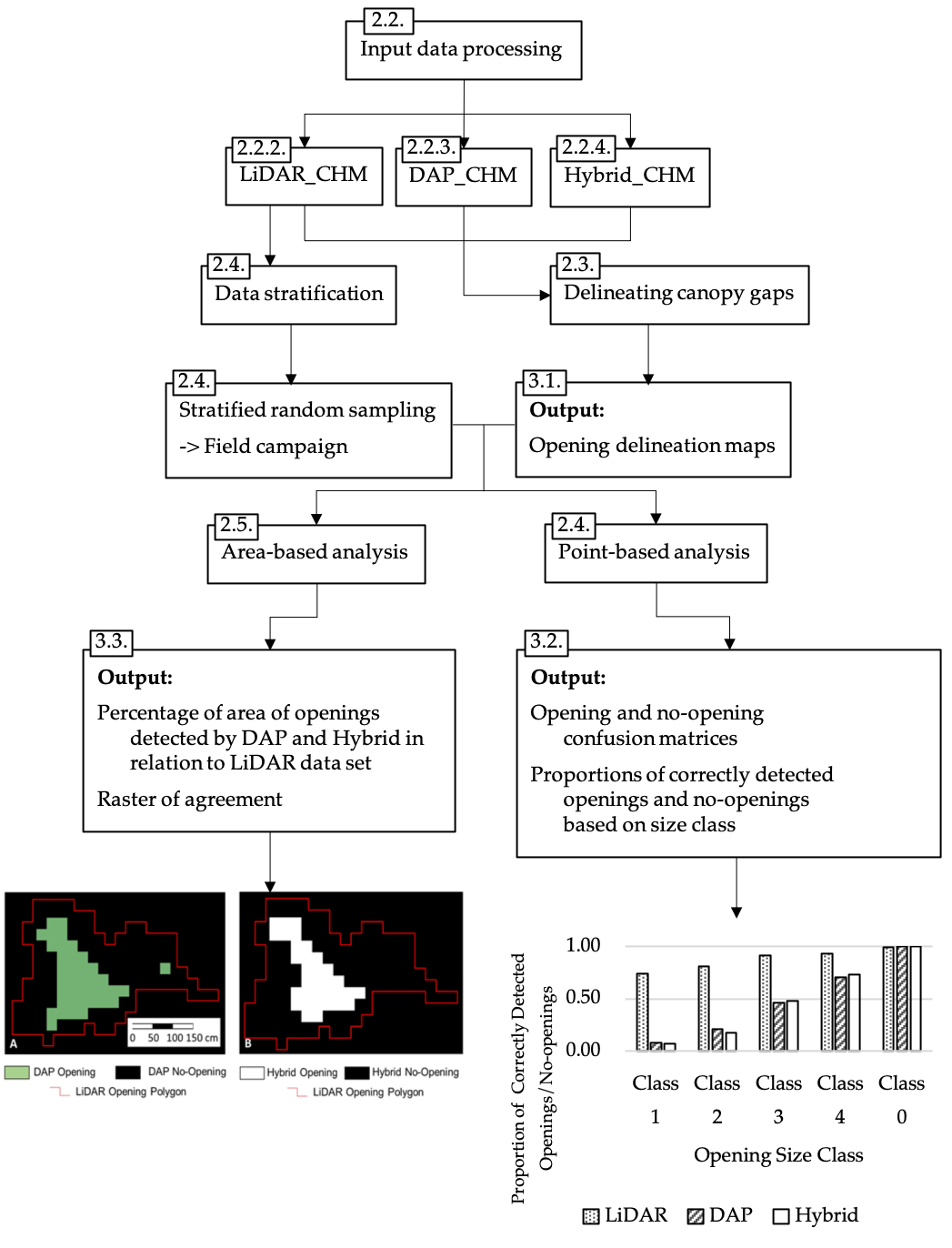
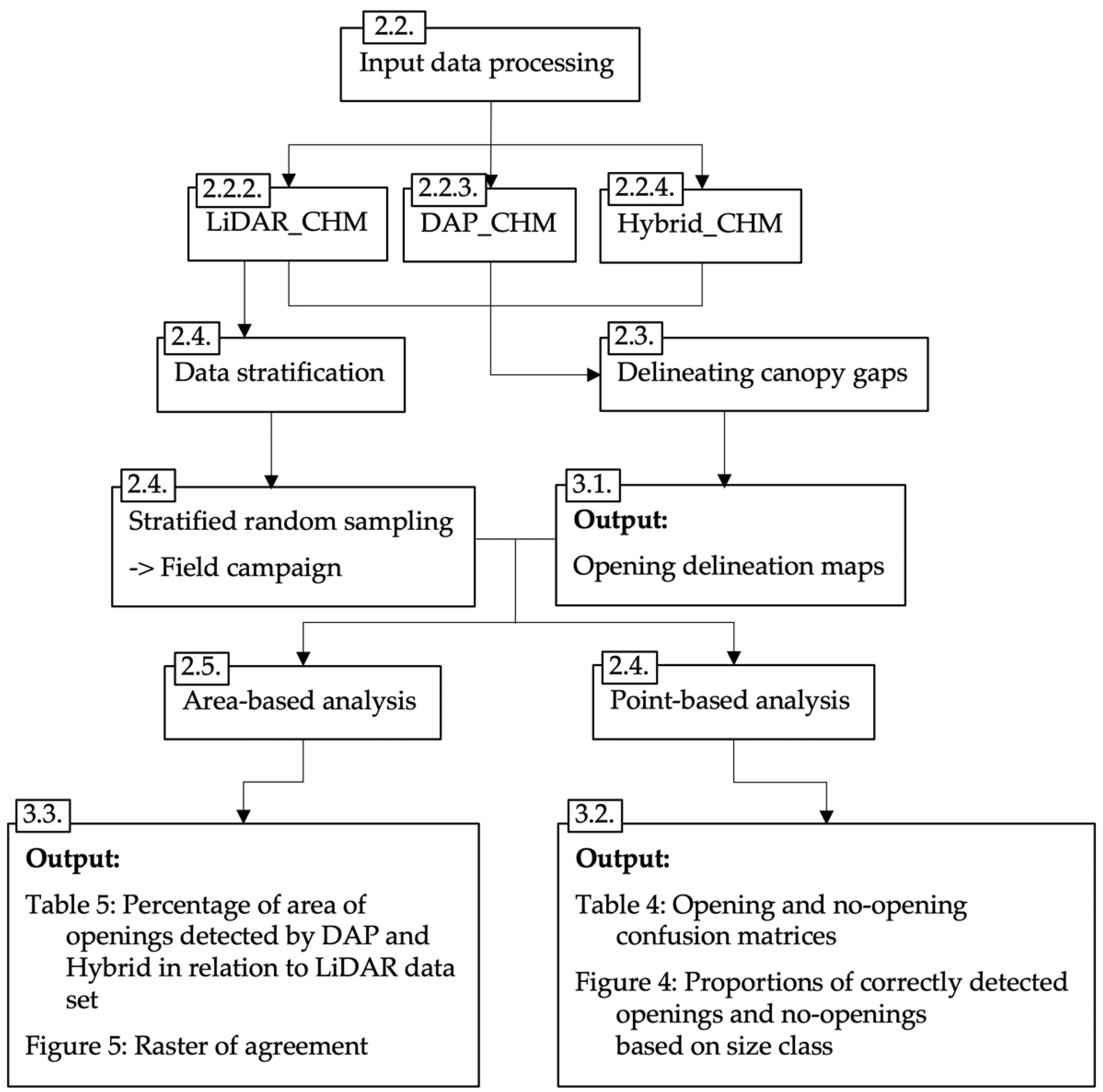
2. Materials and Methods
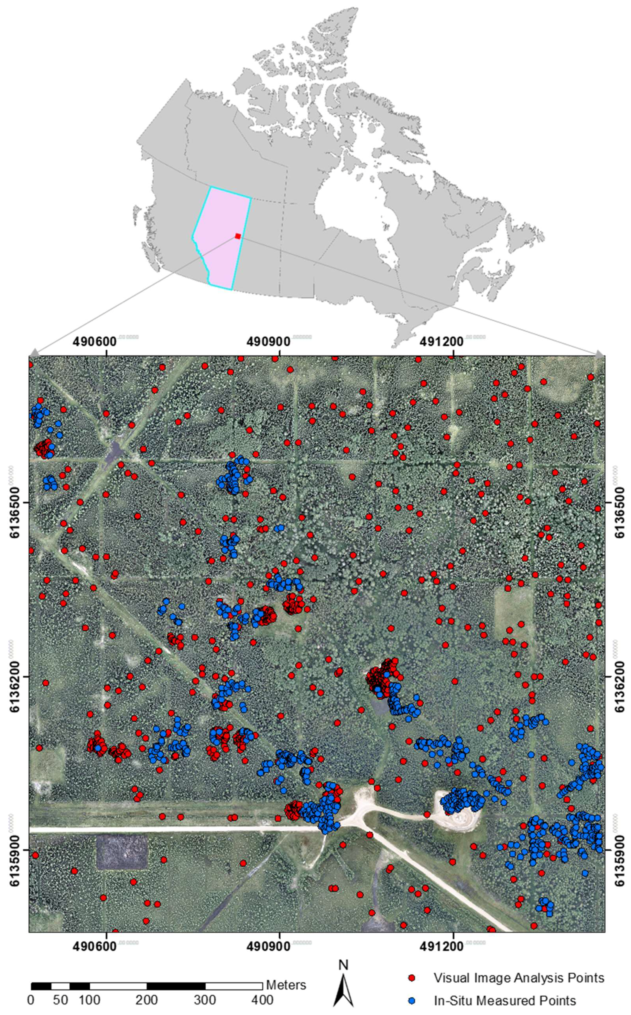
2.1. Study Area
2.2. Remote Sensing Data Collection and Pre-Processing
2.2.1. Remote Sensing Data Collection
2.2.2. LiDAR-Based CHM
2.2.3. DAP-Based CHM
2.2.4. Hybrid CHM
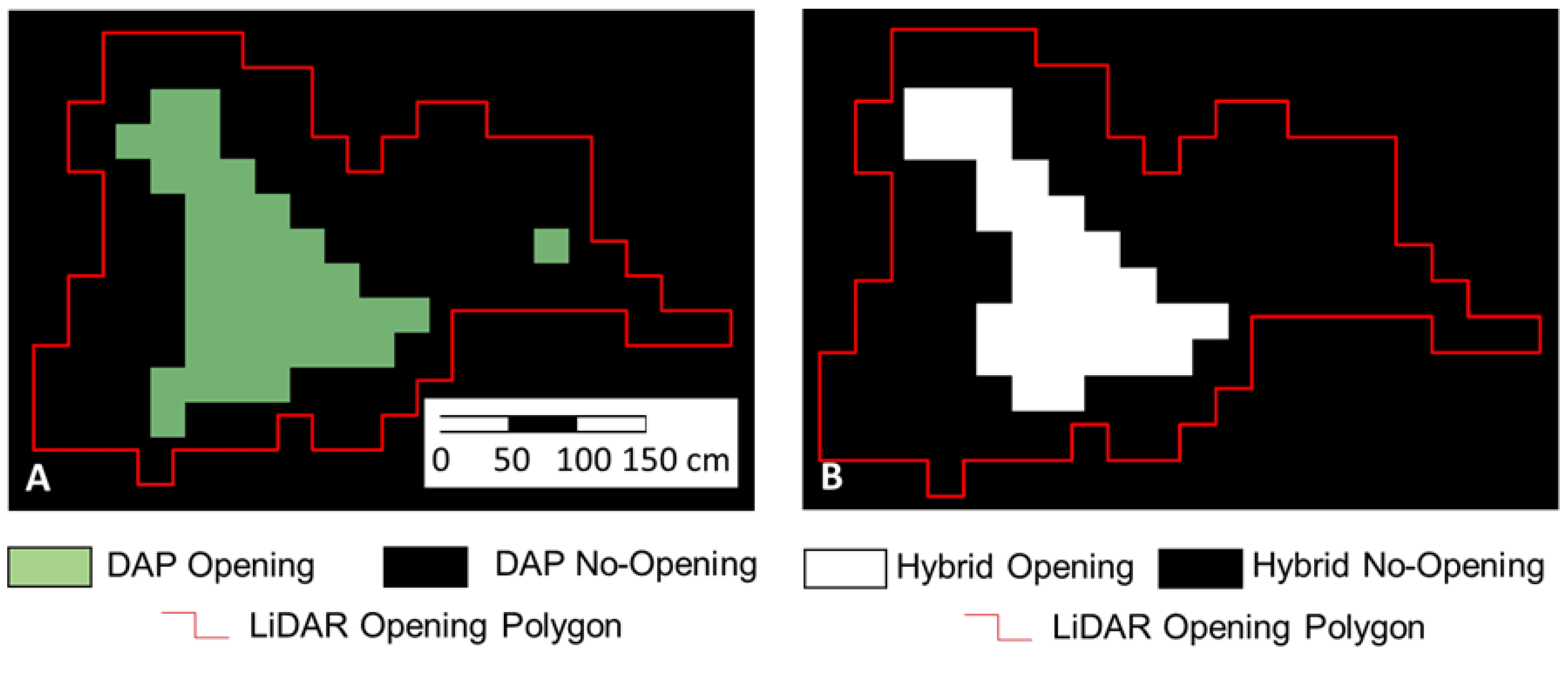
2.3. Delineating Canopy Openings
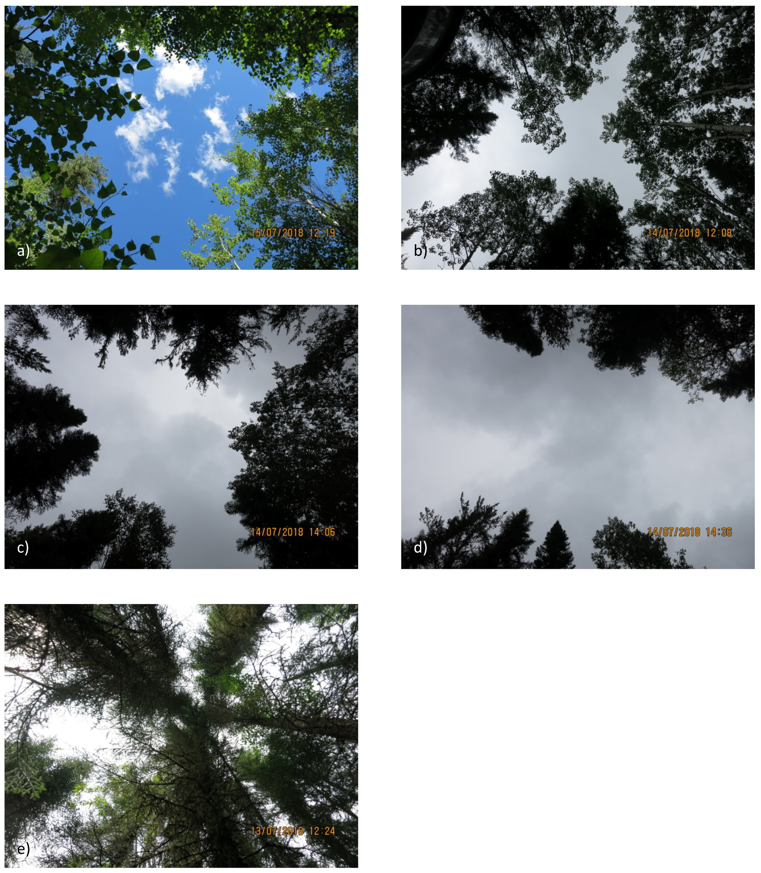
2.4. Validating Canopy Openings—Point-Based Analysis
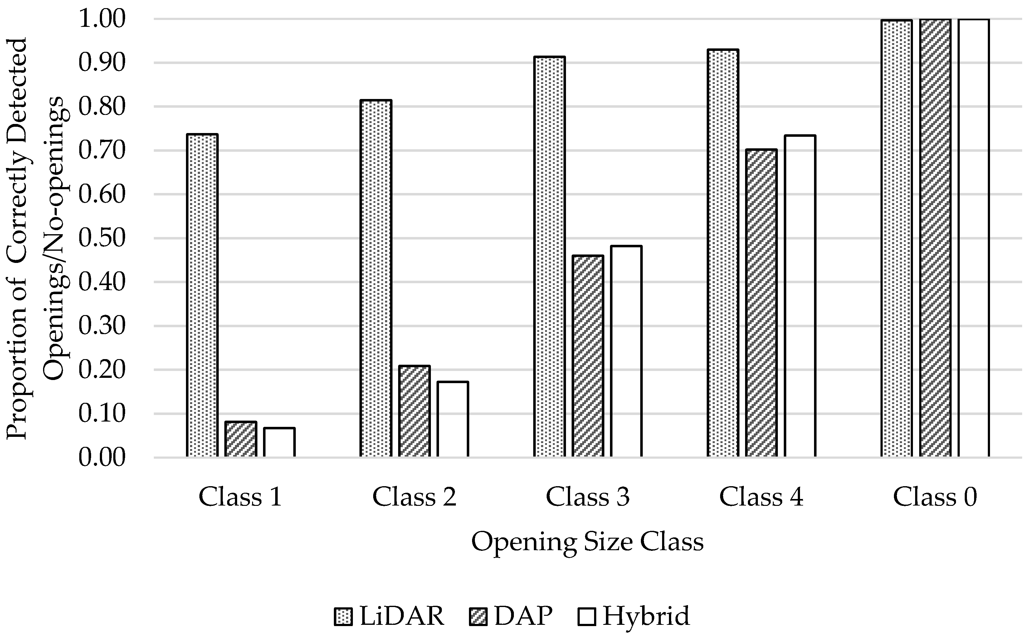
- Opening class 0: No opening (sky above 1.3 m obscured by vegetation)
- Opening class 1: > 0 to 4 m2
- Opening class 2: > 4 to 20 m2
- Opening class 3: > 20 to 200 m2
- Opening class 4: > 200 m2.
- Identify and isolate points that do not have a neighboring point within a 20 m distance.
- Randomly select one point from the remaining points. Identify all remaining points within a 20 m distance of this point and remove them from the list.
- From the remaining points in the list, select another random point. Identify all the points within a 20 m distance of this point and remove them from the list.
- Repeat step 3 until the list is empty.
- Add the randomly selected samples (steps 2–4) and the isolated samples (step 1) together to obtain a complete set of spatially uncorrelated samples.
2.5. Examination of Opening Characteristics—Area-Based Analysis
2.6. Examination of the Value of DAP in Measuring Height
3. Results
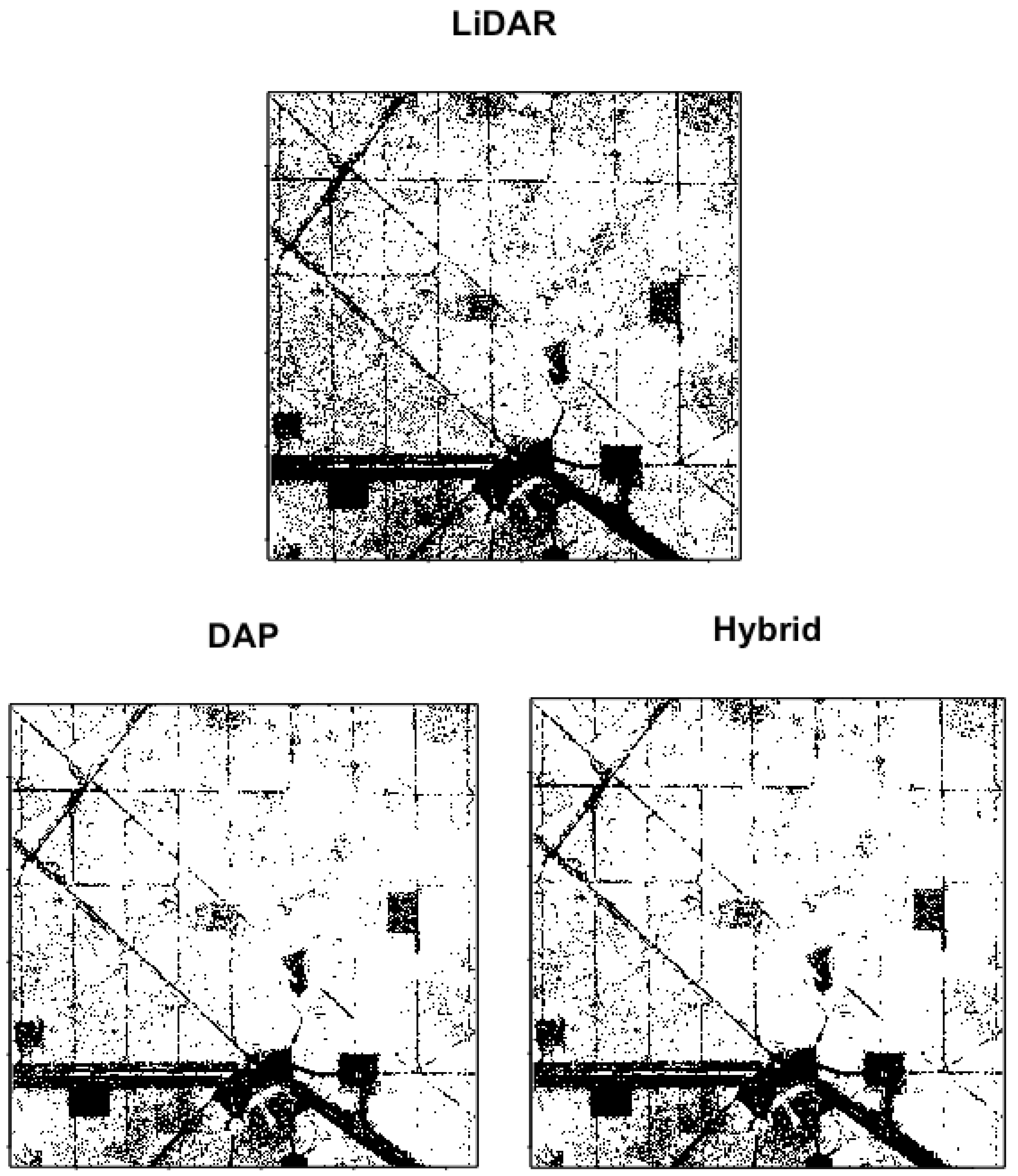
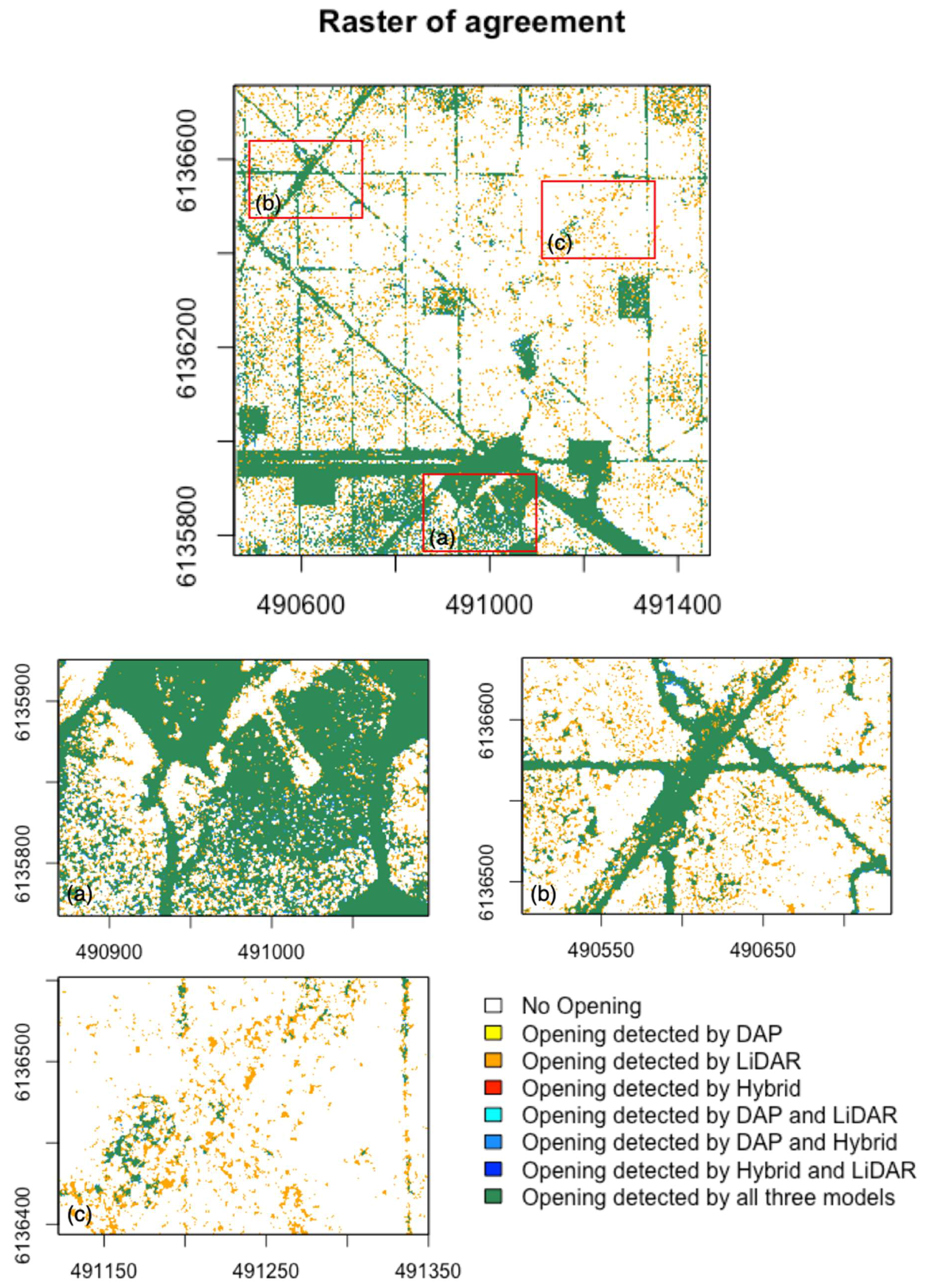
3.1. Opening Maps
3.2. Point-Based Analysis
3.3. Area-Based Analysis
3.4. Value of the Hybrid Model—CHMHybrid vs. CHMDAP Relative to CHMLiDAR
4. Discussion
5. Conclusions
Supplementary Materials
Author Contributions
Funding
Acknowledgments
Conflicts of Interest
References
- Burton, P.J.; Parisien, M.A.; Hicke, J.A.; Hall, R.J.; Freeburn, J.T. Large fires as agents of ecological diversity in the North American boreal forest. Int. J. Wildl. Fire 2008, 17, 754–767. [Google Scholar] [CrossRef]
- Senf, C.; Pflugmacher, D.; Hostert, P.; Seidl, R. Using Landsat time series for characterizing forest disturbance dynamics in the coupled human and natural systems of Central Europe. ISPRS J. Photogramm. Remote Sens. 2017, 130, 453–463. [Google Scholar] [CrossRef] [PubMed]
- Dabros, A.; Pyper, M.; Castilla, G. Seismic lines in the boreal and arctic ecosystems of North America: Environmental impacts, challenges, and opportunities. Environ. Rev. 2018, 16, 1–16. [Google Scholar] [CrossRef]
- Lee, P.; Boutin, S. Persistence and developmental transition of wide seismic lines in the western Boreal Plains of Canada. J. Environ. Manag. 2006, 78, 240–250. [Google Scholar] [CrossRef] [PubMed]
- Schroeder, T.A.; Wulder, M.A.; Healey, S.P.; Moisen, G.G. Mapping wild fire and clearcut harvest disturbances in boreal forests with Landsat time series data. Remote Sens. Environ. 2011, 115, 1421–1433. [Google Scholar] [CrossRef]
- Rahman, M.M.; McDermid, G.J.; Strack, M.; Lovitt, J. A new method to map groundwater table in peatlands using unmanned aerial vehicles. Remote Sens. 2017, 9, 1057. [Google Scholar] [CrossRef]
- Lertzman, K.P.; Sutherland, G.D.; Inselberg, A.; Saunders, S.C. Canopy Gaps and the Landscape Mosaic in a Coastal Temperate Rain Forest. Ecology 1996, 77, 1254–1270. [Google Scholar] [CrossRef]
- White, J.C.; Tompalski, P.; Coops, N.C.; Wulder, M.A. Comparison of airborne laser scanning and digital stereo imagery for characterizing forest canopy gaps in coastal temperate rainforests. Remote Sens. Environ. 2018, 208, 1–14. [Google Scholar] [CrossRef]
- Dabros, A.; Hammond, H.E.J.; Pinzon, J.; Pinno, B.; Langor, D. Edge influence of low-impact seismic lines for oil exploration on upland forest vegetation in northern Alberta (Canada). For. Ecol. Manag. 2017, 400, 278–288. [Google Scholar] [CrossRef]
- Canham, C.D.; Denslow, J.S.; Platt, W.J.; Runkle, J.R.; Spies, T.A.; White, P.S. Light regimes beneath closed canopies and tree-fall gaps in temperate and tropical forests. Can. J. For. Res. 1990, 20, 620–631. [Google Scholar] [CrossRef]
- Feldmann, E.; Drößler, L.; Hauck, M.; Kucbel, S.; Pichler, V.; Leuschner, C. Forest Ecology and Management Canopy gap dynamics and tree understory release in a virgin beech forest, Slovakian Carpathians. For. Ecol. Manag. 2018, 415–416, 38–46. [Google Scholar] [CrossRef]
- Lawton, R.; Putz, F.E. Natural Disturbance and Gap-Phase Regeneration in a Wind-Exposed Tropical Cloud Forest. Ecology 1988, 69, 764–777. [Google Scholar] [CrossRef]
- Runkle, J.R. Guidelines and Sample Protocol for Sampling Forest Gaps; US Department of Agriculture, Forest Service, Pacific Northwest Research Station: Portland, OR, USA, 1992; Volume 283, ISBN 0894192090303.
- Hebblewhite, M. Billion dollar boreal woodland caribou and the biodiversity impacts of the global oil and gas industry. Biol. Conserv. 2017, 206, 102–111. [Google Scholar] [CrossRef]
- Lovitt, J.; Rahman, M.M.; Saraswati, S.; McDermid, G.J.; Strack, M.; Xu, B. UAV remote sensing can reveal the effects of low-impact seismic lines on surface morphology, hydrology, and methane (CH4) release in a boreal treed bog. J. Geophys. Res. Biogeosci. 2018. [Google Scholar] [CrossRef]
- Brokaw, N.V.L. The Definition of Treefall Gap and Its Effect on Measures of Forest Dynamics. Biotropica 1982, 14, 158–160. [Google Scholar] [CrossRef]
- Pickett, S.T.A.; Wu, J.; Cadenasso, M.L. Patch dynamics and the ecology of disturbed ground: A framework for synthesis. In Ecosystems of Disturbed Ground. Ecosystems of the World; Walker, L.R., Ed.; Elsevier: Amsterdam, The Netherlands, 1999; Volume 16, pp. 707–722. [Google Scholar]
- Baret, F.; Clevers, J.G.P.W.; Steven, M.D. The robustness of canopy gap fraction estimates from red and near-infrared reflectances: A comparison of approaches. Remote Sens. Environ. 1995, 54, 141–151. [Google Scholar] [CrossRef]
- Liu, J.; Skidmore, A.K.; Jones, S.; Wang, T.J.; Heurich, M.; Zhu, X.; Shi, Y.F. Large off-nadir scan angle of airborne LiDAR can severely affect the estimates of forest structure metrics. ISPRS J. Photogramm. Remote Sens. 2018, 136, 13–25. [Google Scholar] [CrossRef]
- Cescatti, A. Indirect estimates of canopy gap fraction based on the linear conversion of hemispherical photographs. Agric. For. Meteorol. 2006, 143, 1–12. [Google Scholar] [CrossRef]
- Cohen, W.B.; Spies, T.A.; Fiorella, M. Estimating the age and structure of forests in a multi-ownership landscape of western Oregon, U.S.A. Int. J. Remote Sens. 1995, 16, 721–746. [Google Scholar] [CrossRef]
- Rautiainen, M.; Stenberg, P.; Nilson, T. Estimating Canopy Cover in Scots Pine Stands. Silva Fenn. 2005, 39, 137–142. [Google Scholar] [CrossRef]
- Rehush, N.; Waser, L.T. Assessing the structure of primeval and managed beech forests in the Ukrainian Carpathians using remote sensing. Can. J. For. Res. 2017, 47, 63–72. [Google Scholar] [CrossRef]
- Hobi, M.L.H.; Ginzler, C.G.; Commarmot, B.C.; Bugmann, H. Gap pattern of the largest primeval beech forest of Europe revealed by remote sensing. ESA Ecosph. 2015, 6, 1–15. [Google Scholar] [CrossRef]
- Nyamgeroh, B.B.; Groen, T.A.; Weir, M.J.C.; Dimov, P.; Zlatanov, T. Detection of forest canopy gaps from very high resolution aerial images. Ecol. Indic. 2018, 95, 629–636. [Google Scholar] [CrossRef]
- Vepakomma, U.; St-Onge, B.; Kneeshaw, D. Spatially explicit characterization of boreal forest gap dynamics using multi-temporal lidar data. Remote Sens. Environ. 2008, 112, 2326–2340. [Google Scholar] [CrossRef]
- Gaulton, R.; Malthus, T.J. LiDAR mapping of canopy gaps in continuous cover forests: A comparison of canopy height model and point cloud based techniques. Int. J. Remote Sens. 2010, 31, 1193–1211. [Google Scholar] [CrossRef]
- Vehmas, M.; Packalén, P.; Maltamo, M.; Eerikäinen, K. Using airborne laser scanning data for detecting canopy gaps and their understory type in mature boreal forest. Ann. For. Sci. 2011, 68, 825–833. [Google Scholar] [CrossRef]
- Bonnet, S.; Gaulton, R.; Lehaire, F.; Lejeune, P. Canopy gap mapping from airborne laser scanning: An assessment of the positional and geometrical accuracy. Remote Sens. 2015, 7, 11267–11294. [Google Scholar] [CrossRef]
- Asner, G.P.; Kellner, J.R.; Kennedy-Bowdoin, T.; Knapp, D.E.; Anderson, C.; Martin, R.E. Forest Canopy Gap Distributions in the Southern Peruvian Amazon. PLoS ONE 2013, 8, e60875. [Google Scholar] [CrossRef] [PubMed]
- Koukoulas, S.; Blackburn, G.A. Quantifying the spatial properties of forest canopy gaps using LiDAR imagery and GIS. Int. J. Remote Sens. 2004, 25, 3049–3071. [Google Scholar] [CrossRef]
- Koukoulas, S.; Blackburn, G.A. Spatial relationships between tree species and gap characteristics in broad-leaved deciduous woodland. J. Veg. Sci. 2005, 16, 587–596. [Google Scholar] [CrossRef]
- Lefsky, M.A.; Cohen, W.B.; Parker, G.G.; Harding, D.J. Lidar Remote Sensing for Ecosystem Studies. Bioscience 2002, 52, 19–30. [Google Scholar] [CrossRef]
- Næsset, E. Vertical height errors in digital terrain models derived from airborne laser scanner data in a boreal-alpine ecotone in Norway. Remote Sens. 2015, 7, 4702–4725. [Google Scholar] [CrossRef]
- Leberl, F.; Irschara, A.; Pock, T.; Meixner, P.; Gruber, M.; Scholz, S.; Wiechert, A. Point Clouds: Lidar versus 3D Vision. Photogramm. Eng. Remote Sens. 2010, 76, 1123–1134. [Google Scholar] [CrossRef]
- St-Onge, B.; Vega, C.; Fournier, R.A.; Hu, Y. Mapping canopy height using a combination of digital stereo-photogrammetry and lidar. Int. J. Remote Sens. 2008, 29, 3343–3364. [Google Scholar] [CrossRef]
- Filipelli, S.K.; Lefsky, M.A.; Rocca, M.E. Comparison and integration of lidar and photogrammetric point clouds for mapping pre-fire forest structure. Remote Sens. Environ. 2019, 224, 152–166. [Google Scholar] [CrossRef]
- Holopainen, M.; Vastaranta, M.; Karjalainen, M.; Karila, K.; Kaasalainen, S.; Honkavaara, E.; Hyyppä, J. Forest Inventory Attribute Estimation Using Airborne Laser Scanning, Aerial Stereo Imagery, Radargrammetry and Interferometry–Finnish Experiences of the 3D Techniques. ISPRS Ann. Photogramm. Remote Sens. Spat. Inf. Sci. 2015, II-3/W4, 63–69. [Google Scholar] [CrossRef]
- White, J.C.; Wulder, M.A.; Vastaranta, M.; Coops, N.C.; Pitt, D.; Woods, M. The utility of image-based point clouds for forest inventory: A comparison with airborne laser scanning. Forests 2013, 4, 518–536. [Google Scholar] [CrossRef]
- Remondino, F.; Spera, M.G.; Nocerino, E.; Menna, F.; Nex, F. State of the art in high density image matching. Photogramm. Rec. 2014, 29, 144–166. [Google Scholar] [CrossRef] [Green Version]
- Zhang, K. Identification of gaps in mangrove forests with airborne LIDAR. Remote Sens. Environ. 2008, 112, 2309–2325. [Google Scholar] [CrossRef]
- Wallace, L.; Lucieer, A.; Malenovsky, Z.; Turner, D. Assessment of Forest Structure Using Two UAV Techniques: A Comparison of Airborne Laser Scanning and Structure from Motion (SfM) Point Clouds. Forests 2016, 7, 62. [Google Scholar] [CrossRef]
- Swinfield, T.; Lindsell, J.A.; Williams, J.V.; Harrison, R.D.; Agustiono, H.; Gemita, E.; Schonlieb, C.B.; Coomes, D.A. Accurate Measurement of Tropical Forest Canopy Heights and Aboveground Carbon Using Structure From Motion. Remote Sens. 2019, 11, 928. [Google Scholar] [CrossRef]
- Vastaranta, M.; Yrttimaa, T.; Saarinen, N.; Yu, X.W.; Karjalainen, M.; Nurminen, K.; Karila, K.; Kankare, V.; Luoma, V.; Pyorala, J.; et al. Airborne Laser Scanning Outperforms the Alternative 3D Techniques in Capturing Variation in Tree Height and Forest Density in Southern Boreal Forests. Balt. For. 2018, 24, 268–277. [Google Scholar]
- Cao, L.; Liu, H.; Fu, X.Y.; Zhang, Z.N.; Shen, X.; Ruan, H.H. Comparison of UAV LiDAR and Digital Aerial Photogrammetry Point Clouds for Estimating Forest Structural Attributes in Subtropical Planted Forests. Forests 2019, 10, 145. [Google Scholar] [CrossRef]
- Graham, A.; Coops, N.C.; Wilcox, M.; Plowright, A. Evaluation of Ground Surface Models Derived from Unmanned Aerial Systems with Digital Aerial Photogrammetry in a Disturbed Conifer Forest. Remote Sens. 2019, 11, 84. [Google Scholar] [CrossRef]
- Iqbal, I.A.; Osborn, J.; Lucieer, A. A comparison of area-based forest attributes derived from airborne laser scanner, small-format and medium-format digital aerial photography. Int. J. Appl. Earth Obs. Geoinf. 2019, 76, 231–241. [Google Scholar] [CrossRef]
- Swetnam, T.L.; Gillan, J.K.; Sankey, T.T.; Mcclaran, M.P.; Nichols, M.H.; Heilman, P.; Mcvay, J. Considerations for Achieving Cross-Platform Point Cloud Data Fusion across Different Dryland Ecosystem Structural States. Front. Plant Sci. 2018, 8, 1–13. [Google Scholar] [CrossRef] [PubMed]
- Pearse, G.D.; Dash, J.P.; Persson, H.J.; Watt, M.S. Comparison of high-density LiDAR and satellite photogrammetry for forest inventory. ISPRS J. Photogramm. Remote Sens. 2018, 142, 257–267. [Google Scholar] [CrossRef]
- Fankhauser, K.E.; Strigul, N.S.; Gatziolis, D. Augmentation of Traditional Forest Inventory and Airborne Laser Scanning with Unmanned Aerial Systems and Photogrammetry for Forest Monitoring. Remote Sens. 2018, 10, 1562. [Google Scholar] [CrossRef]
- St-Onge, B.; Audet, F.-A.; Bégin, J. Characterizing the Height Structure and Composition of a Boreal Forest Using an Individual Tree Crown Approach Applied to Photogrammetric Point Clouds. Forests 2015, 6, 3899–3922. [Google Scholar] [CrossRef]
- White, J.C.; Stepper, C.; Tompalski, P.; Coops, N.C.; Wulder, M.A. Comparing ALS and image-based point cloud metrics and modelled forest inventory attributes in a complex coastal forest environment. Forests 2015, 6, 3704–3732. [Google Scholar] [CrossRef]
- Ni, W.; Jon, K.; Zhang, Z.; Sun, G. Features of point clouds synthesized from multi-view ALOS/PRISM data and comparisons with LiDAR data in forested areas. Remote Sens. Environ. 2014, 149, 47–57. [Google Scholar] [CrossRef] [Green Version]
- Rahlf, J.; Breidenbach, J.; Solberg, S.; Naesset, E.; Astrup, R. Comparison of four types of 3D data for timber volume estimation. Remote Sens. Environ. 2014, 155, 325–333. [Google Scholar] [CrossRef]
- Vastaranta, M.; Wulder, M.A.; White, J.C.; Pekkarinen, A.; Tuominen, S.; Ginzler, C.; Kankare, V.; Holopainen, M.; Hyyppä, J.; Hyyppä, H. Airborne laser scanning and digital stereo imagery measures of forest structure: Comparative results and implications to forest mapping and inventory update. Can. J. Remote Sens. 2013, 39, 382–395. [Google Scholar] [CrossRef]
- Gil, A.L.; Núñez-Casillas, L.; Isenburg, M.; Benito, A.A.; Bello, J.J.R.; Arbelo, M. A comparison between LiDAR and photogrammetry digital terrain models in a forest area on Tenerife Island. Can. J. Remote Sens. 2013, 39, 396–409. [Google Scholar]
- Bohlin, J.; Wallerman, J.; Fransson, J.E.S. Forest variable estimation using photogrammetric matching of digital aerial images in combination with a high-resolution DEM. Scand. J. For. Res. 2012, 27, 692–699. [Google Scholar] [CrossRef]
- Järnstedt, J.; Pekkarinen, A.; Tuominen, S.; Ginzler, C.; Holopainen, M.; Viitala, R. Forest variable estimation using a high-resolution digital surface model. ISPRS J. Photogramm. Remote Sens. 2012, 74, 78–84. [Google Scholar] [CrossRef]
- Mccarthy, J. Gap dynamics of forest trees: A review with particular attention to boreal forests. Environ. Rev. 2001, 9, 1–59. [Google Scholar] [CrossRef]
- Kottek, M.; Grieser, J.; Beck, C.; Rudolf, B.; Rubel, F. World map of the Köppen-Geiger climate classification updated. Meteorol. Z. 2006, 15, 259–263. [Google Scholar] [CrossRef]
- Downing, D.J.; Pettapiece, W.W. Natural Regions and Subregions of Alberta; Government of Alberta: Edmonton, AB, Canada, 2006; ISBN 0778545725.
- Westoby, M.J.; Brasington, J.; Glasser, N.F.; Hambrey, M.J.; Reynolds, J.M. “Structure -from- Motion” photogrammetry: A low -cost, effective tool for geoscience applications Introduction. Geomorphology 2012, 179, 300–314. [Google Scholar] [CrossRef]
- Kershaw, J.A.; Ducey, J.M.J.; Beers, T.W.; Husch, B. Forest Mensuration, 5th ed.; John Wiley & Sons: Chichester, UK; Hoboken, NJ, USA, 2016. [Google Scholar]
- Chen, S.; McDermid, G.J.; Castilla, G.; Linke, J. Measuring vegetation height in linear disturbances in the boreal forest with UAV photogrammetry. Remote Sens. 2017, 9, 1257. [Google Scholar] [CrossRef]
- Zielewska-Büttner, K.; Adler, P.; Ehmann, M.; Braunisch, V. Automated detection of forest gaps in spruce dominated stands using canopy height models derived from stereo aerial Imagery. Remote Sens. 2016, 8, 175. [Google Scholar] [CrossRef]
- Lovitt, J.; Rahman, M.M.; McDermid, G.J. Assessing the value of UAV photogrammetry for characterizing terrain in complex peatlands. Remote Sens. 2017, 9, 1–13. [Google Scholar]


| Publication | Location | Forest Type | Forest Attribute | Investigated Canopy Openings? |
|---|---|---|---|---|
| Swinfield et al., 2019 [43] | Sumatra, Indonesia | Lowland tropical forest | Tree height, biomass, carbon density | No |
| Vastaranta et al., 2018 [44] | Finland | Boreal forest | Forest height, tree density, tree height | No |
| Cao et al., 2019 [45] | Eastern China | Subtropical planted forest | Diameter at breast height, Lorey’s height, basal area, stem density, biomass, volume | No |
| Filippelli et al., 2019 [37] | Colorado, USA | Montane coniferous | Biomass, basal area, bulk density, Lorey’s height, maximum height | No |
| Graham et al., 2019 [46] | British Columbia, Canada | Interior cedar hemlock | Terrain | No |
| Iqbal et al., 2019 [47] | Tasmania | Pine plantation | Basal area, stocking, stem volume | No |
| Swetnam et al., 2018 [48] | Arizona, USA | Chihuahuan desert scrub, and semi-arid desert grassland | Terrain, vegetation height | No |
| White et al., 2018 [8] | British Columbia, Canada | Coastal temperate rainforest | Canopy gaps | YES |
| Pearse et al., 2018 [49] | New Zealand | Pine plantation | Stand height, density, basal area, volume | No |
| Fankhauser et al., 2018 [50] | Various US states | Various | Tree counts, tree height | No |
| Wallace et al., 2016 [42] | Tasmania, Australia | Eucalypt forest | Terrain, canopy cover, vertical canopy profile, stem location, tree height | No |
| St-Onge et al., 2015 [51] | Quebec, Canada | Boreal forest | Tree crowns, species, height | No |
| White et al., 2015 [52] | British Columbia, Canada | Coastal temperate rainforest | Tree height, basal area, volume | No |
| Ni et al., 2014 [53] | Main, USA | Northern hardwood | Canopy height | |
| Rahlf et al., 2014 [54] | Southern Norway | Boreal forest | Timber volume | No |
| Vastaranta et al., 2013 [55] | Finland | Boreal forest | Tree volume, diameter, basal area, biomass | No |
| Gil et al., 2013 [56] | Canary Islands, Spain | Tropical pine forest | Terrain | No |
| Bohlin et al., 2012 [57] | Sweden | Boreal forest | Tree height, stem volume, basal area | No |
| Järnstedt et al., 2012 [58] | Finland | Boreal forest | Mean tree height, dominant tree height, basal area, volume | No |
| St-Onge et al., 2008 [36] | New Brunswick and Quebec, Canada | Balsam fir forest, Boreal forest | Canopy height | No |
| Number of Samples | ||
|---|---|---|
| Opening Class | Disturbed | Undisturbed |
| 0 | 100 | 300 |
| 1 | 116 | 102 |
| 2 | 36 | 30 |
| 3 | 69 | 104 |
| 4 | 396 | 582 |
| Total | 717 | 1118 |
| Class 0 | Class 1 | Class 2 | Class 3 | Class 4 | Total | |
|---|---|---|---|---|---|---|
| Mean Number of Samples | 207 | 32 | 19 | 25 | 73 | 358 |
| Standard Deviation | 3.86 | 3.68 | 2.75 | 3.38 | 4.07 | 4.81 |
| Method | Overall Accuracy * (%) | Opening | No-Opening | Kappa | ||
|---|---|---|---|---|---|---|
| Omission Error (%) | Commission Error (%) | Omission Error (%) | Commission Error (%) | |||
| LiDAR | 94.4 | 12.3 | 0.5 | 0.3 | 8.6 | 0.88 |
| DAP | 77.4 | 53.7 | 0.1 | 0.0 | 28.1 | 0.50 |
| Hybrid | 77.8 | 52.6 | 0.1 | 0.0 | 27.7 | 0.51 |
| Opening Class | 0–4 m2 | 4–20 m2 | 20–200 m2 | >200 m2 | |||||
|---|---|---|---|---|---|---|---|---|---|
| % Area Covered | DAP | Hybrid | DAP | Hybrid | DAP | Hybrid | DAP | Hybrid | |
| Undetected | 96.4 | 97.3 | 44.5 | 43.7 | 7.7 | 8.4 | 0.0 | 0.0 | |
| <20% | 1.8 | 1.8 | 35.4 | 33.7 | 24.7 | 19.7 | 0.0 | 0.0 | |
| 20–40% | 0.7 | 0.5 | 13.4 | 15.0 | 40.0 | 38.0 | 10.2 | 6.1 | |
| 40–60% | 0.3 | 0.2 | 5.6 | 6.3 | 21.6 | 25.6 | 34.7 | 26.5 | |
| 60–80% | 0.2 | 0.1 | 1.0 | 1.1 | 5.8 | 7.7 | 51.0 | 59.2 | |
| 80–100% | 0.6 | 0.2 | 0.2 | 0.3 | 0.3 | 0.6 | 4.1 | 8.2 | |
© 2019 by the authors. Licensee MDPI, Basel, Switzerland. This article is an open access article distributed under the terms and conditions of the Creative Commons Attribution (CC BY) license (http://creativecommons.org/licenses/by/4.0/).
Share and Cite
Dietmaier, A.; McDermid, G.J.; Rahman, M.M.; Linke, J.; Ludwig, R. Comparison of LiDAR and Digital Aerial Photogrammetry for Characterizing Canopy Openings in the Boreal Forest of Northern Alberta. Remote Sens. 2019, 11, 1919. https://doi.org/10.3390/rs11161919
Dietmaier A, McDermid GJ, Rahman MM, Linke J, Ludwig R. Comparison of LiDAR and Digital Aerial Photogrammetry for Characterizing Canopy Openings in the Boreal Forest of Northern Alberta. Remote Sensing. 2019; 11(16):1919. https://doi.org/10.3390/rs11161919
Chicago/Turabian StyleDietmaier, Annette, Gregory J. McDermid, Mir Mustafizur Rahman, Julia Linke, and Ralf Ludwig. 2019. "Comparison of LiDAR and Digital Aerial Photogrammetry for Characterizing Canopy Openings in the Boreal Forest of Northern Alberta" Remote Sensing 11, no. 16: 1919. https://doi.org/10.3390/rs11161919