A Combination of PROBA-V/MODIS-Based Products with Sentinel-1 SAR Data for Detecting Wet and Dry Snow Cover in Mountainous Areas


Abstract
:
1. Introduction
2. Study Areas and Dataset
2.1. Study Areas
2.2. SAR and Optical Imagery
2.3. Auxiliary Data
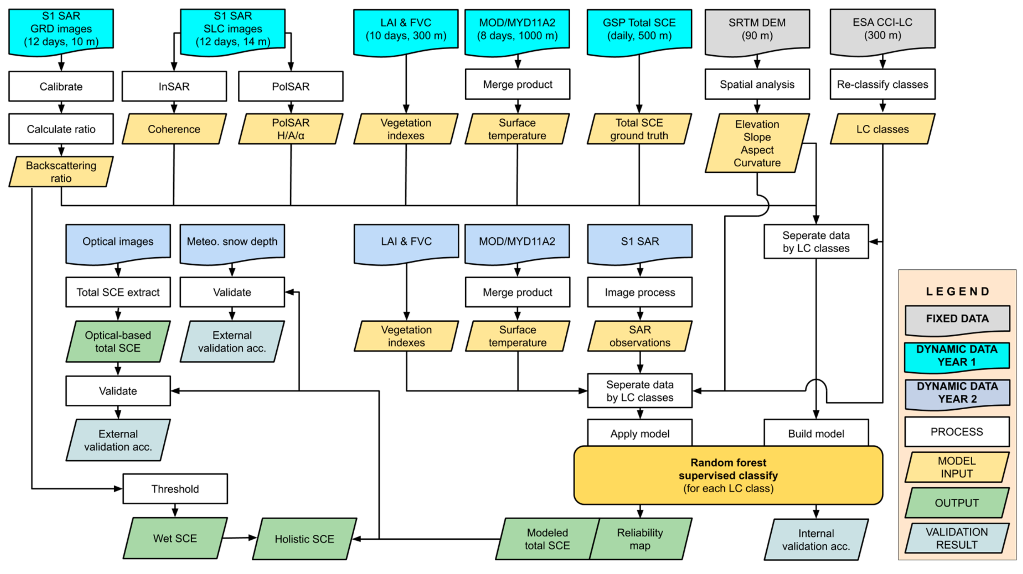
3. Methodology
4. Results
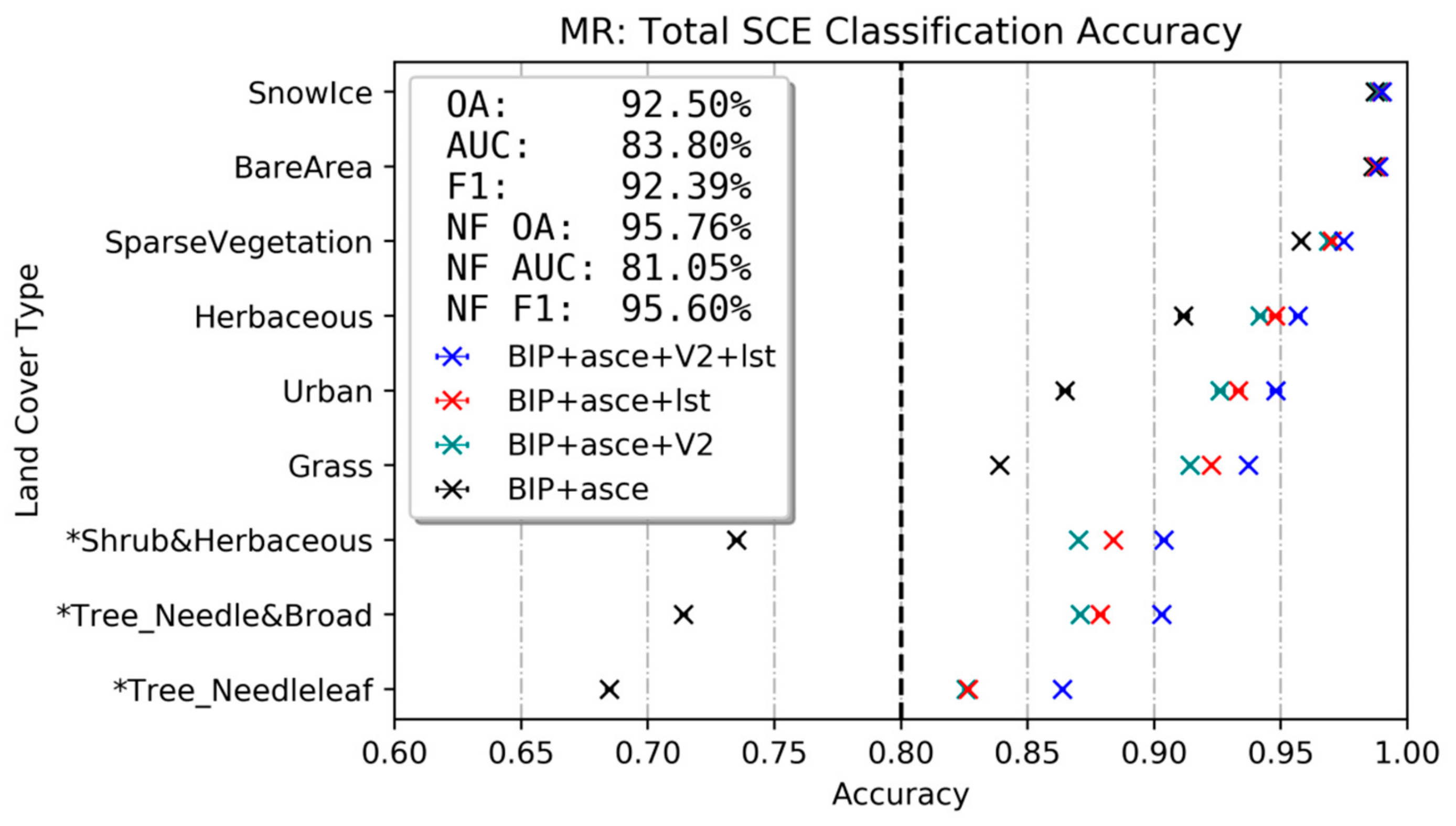
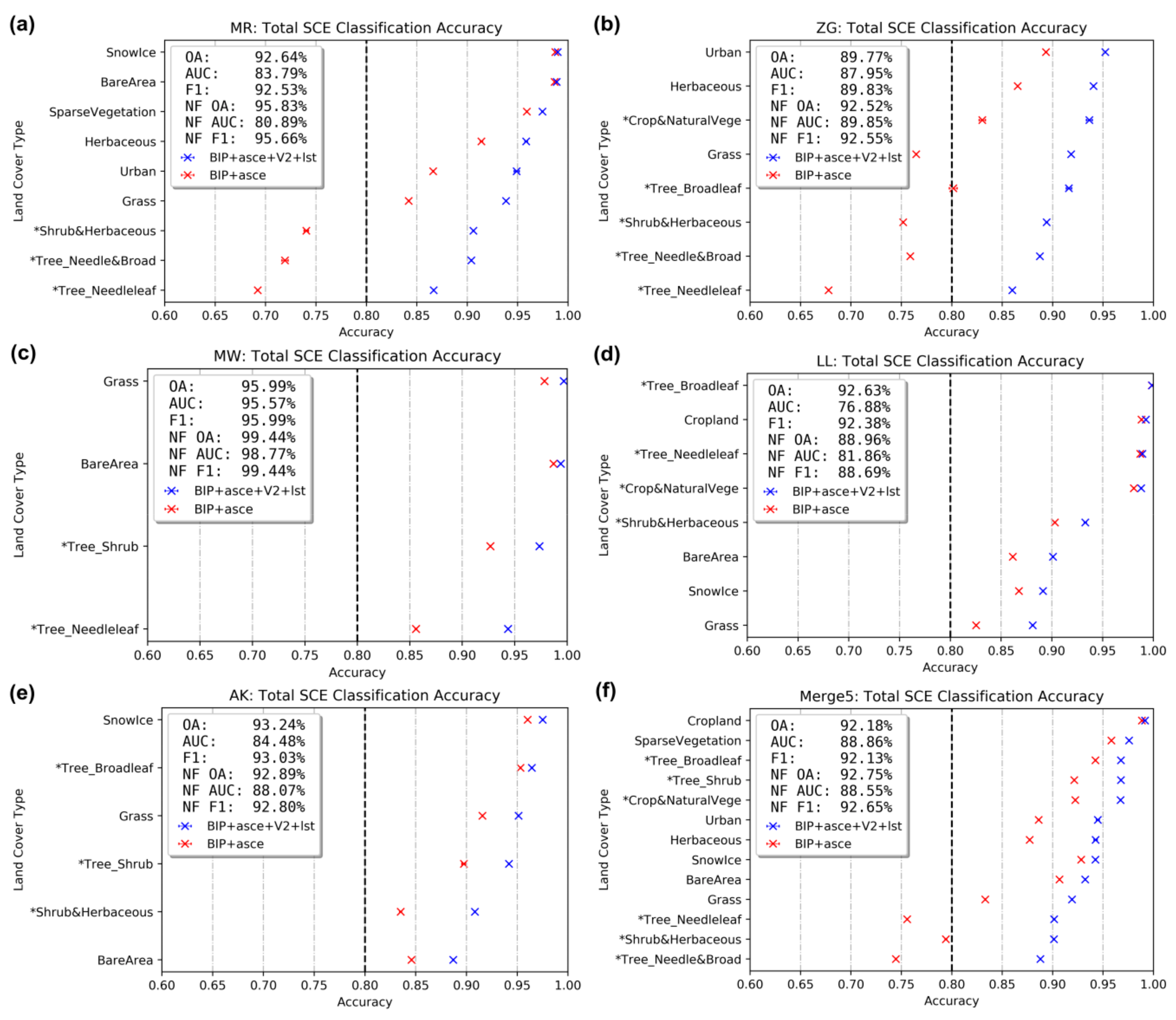
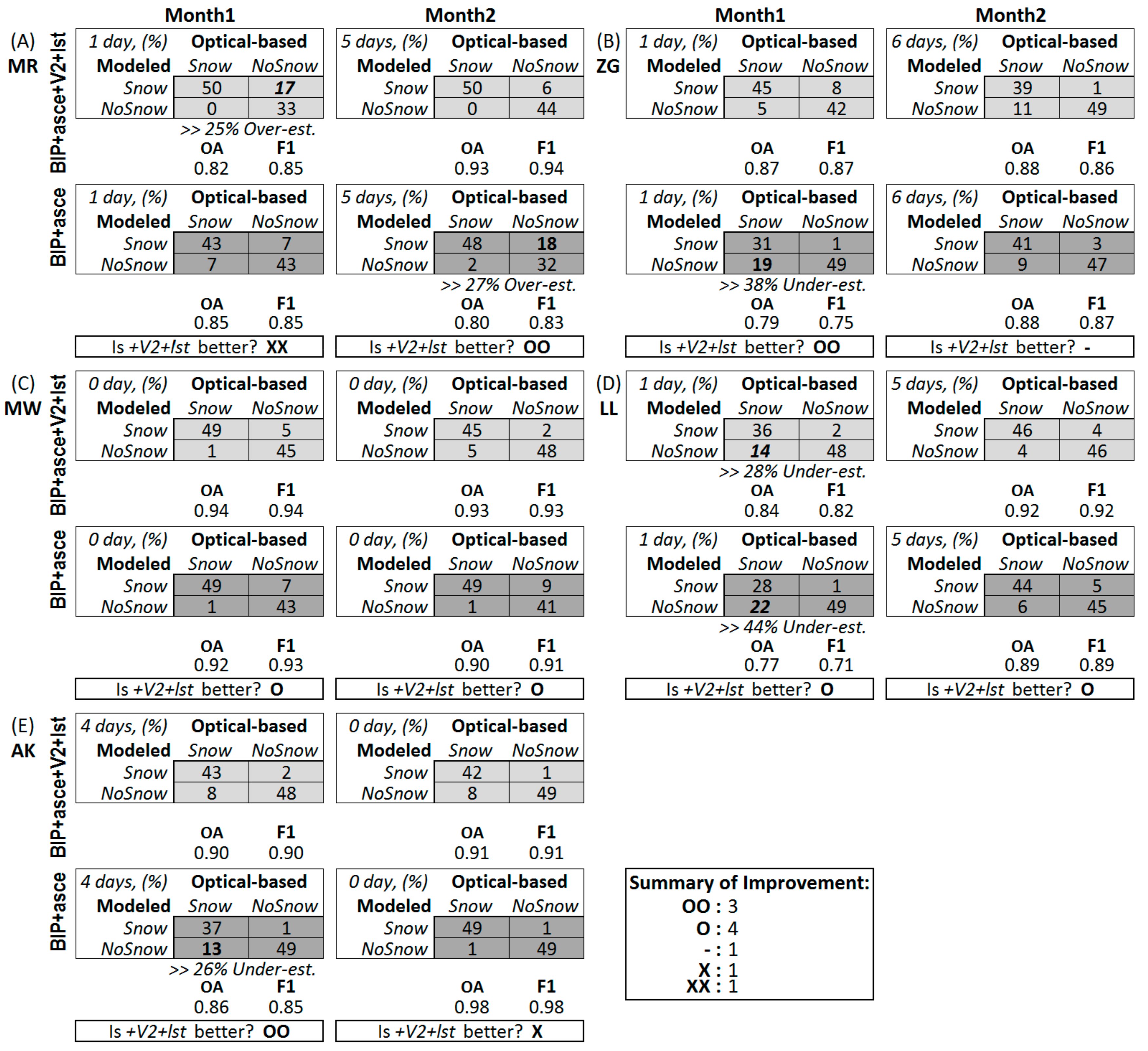
4.1. Accuracy Assessment of the Modeled Total SCE
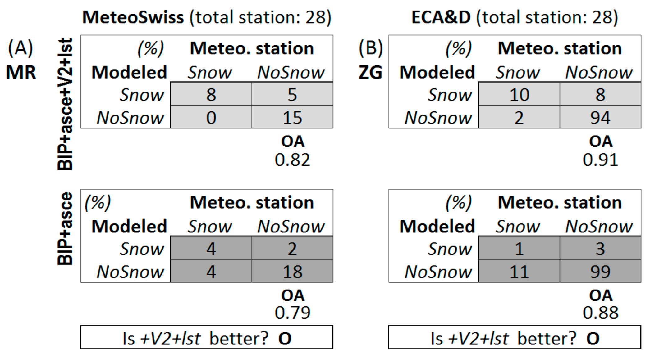
4.2. External Validations with Optical-Based SCE and Snow Depth Records
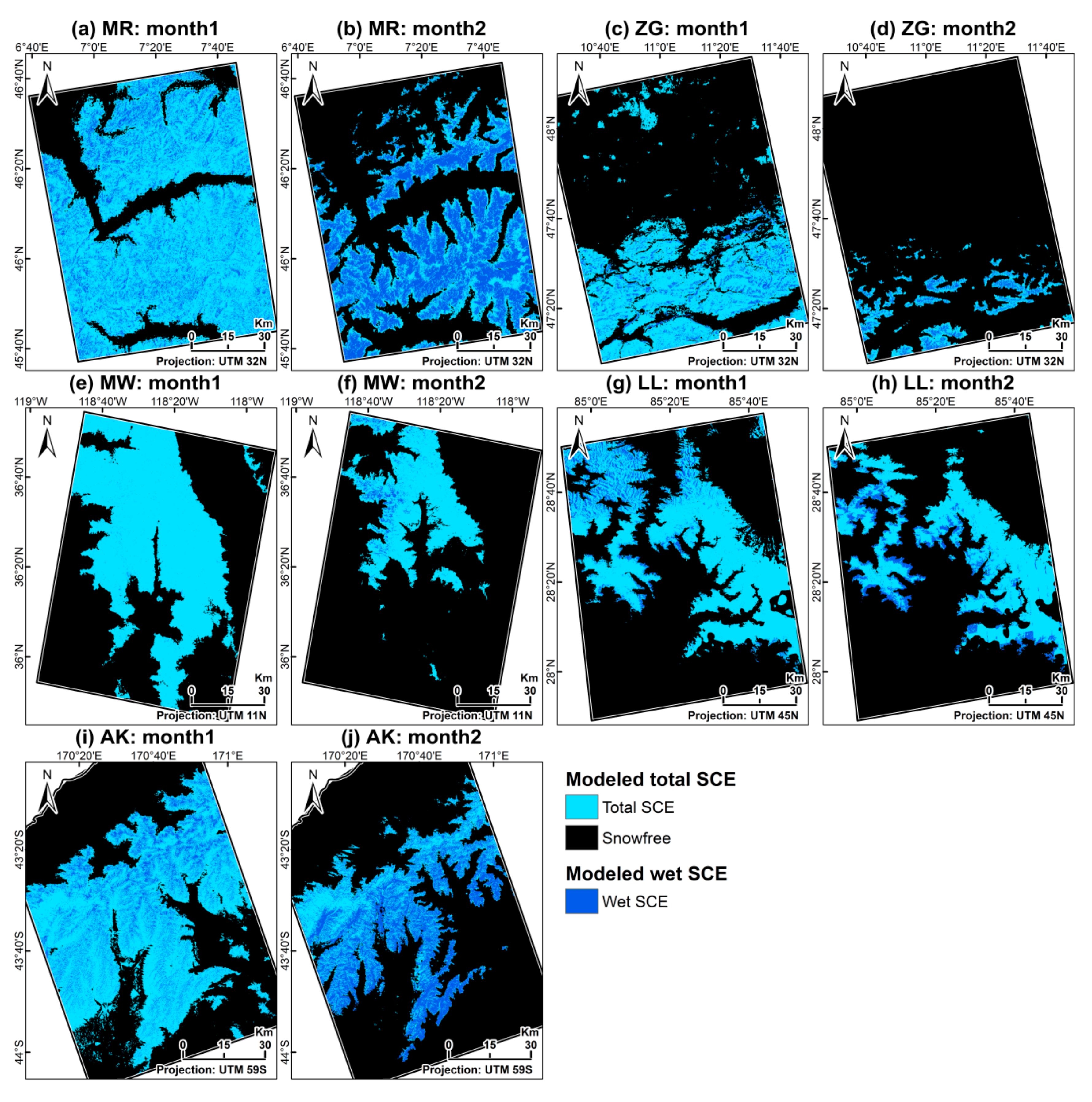
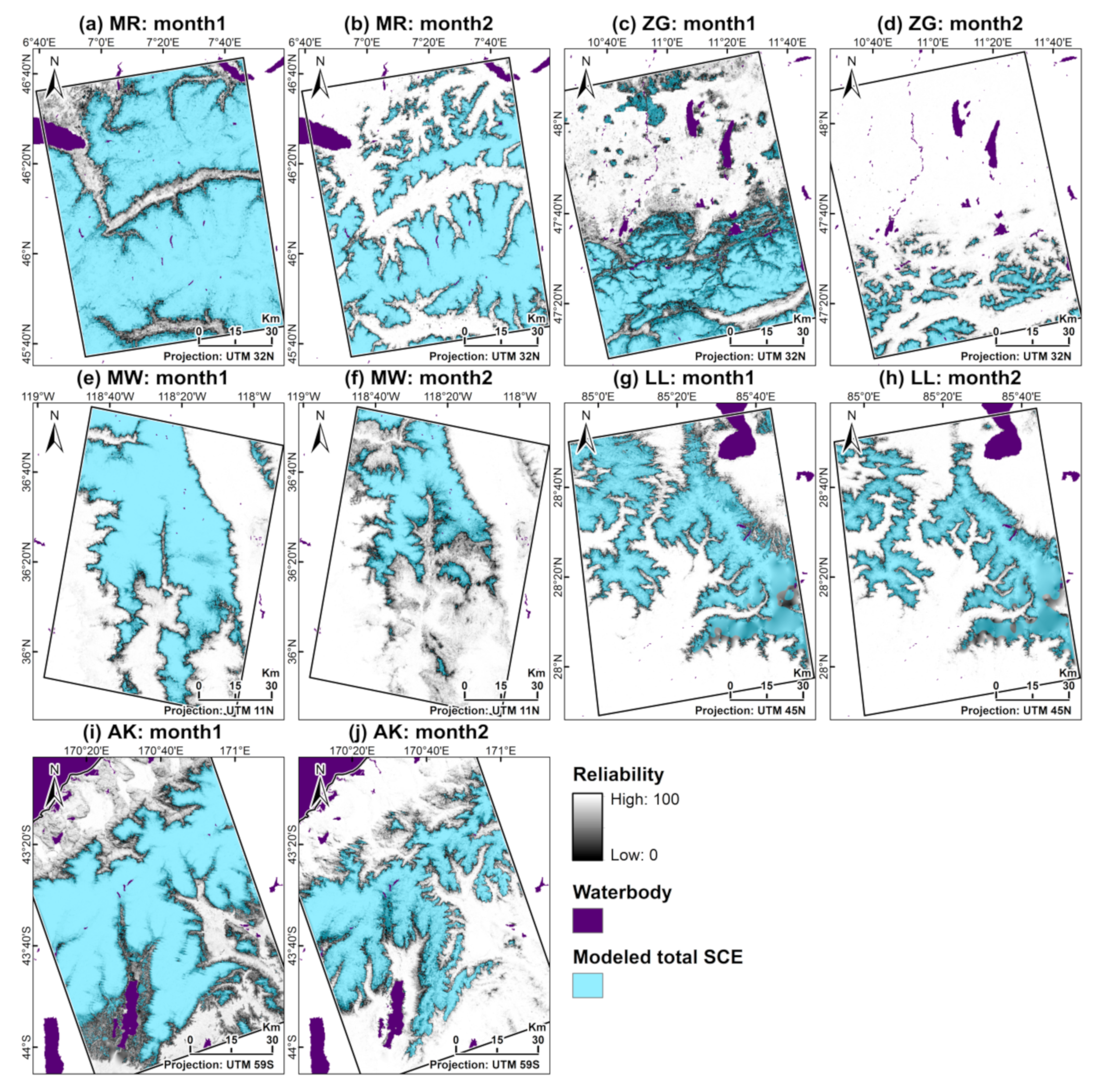
4.3. Holistic Wet and Dry SCE Maps with Reliability Maps
5. Discussion
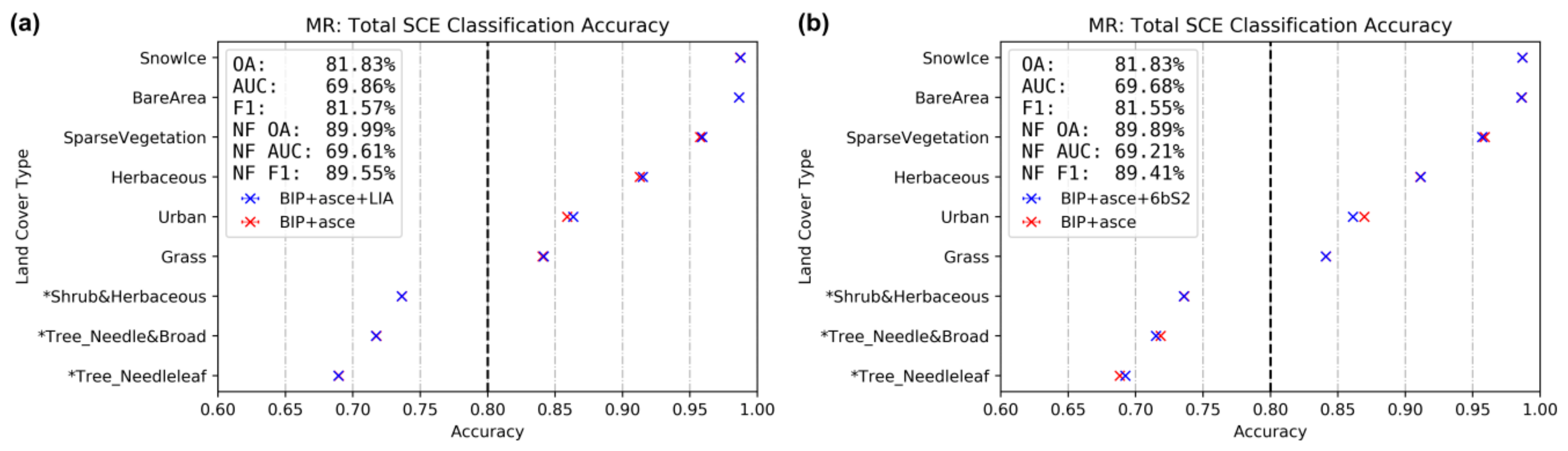
5.1. The Influence of Different Input Variables Combinations to Classification Accuracy
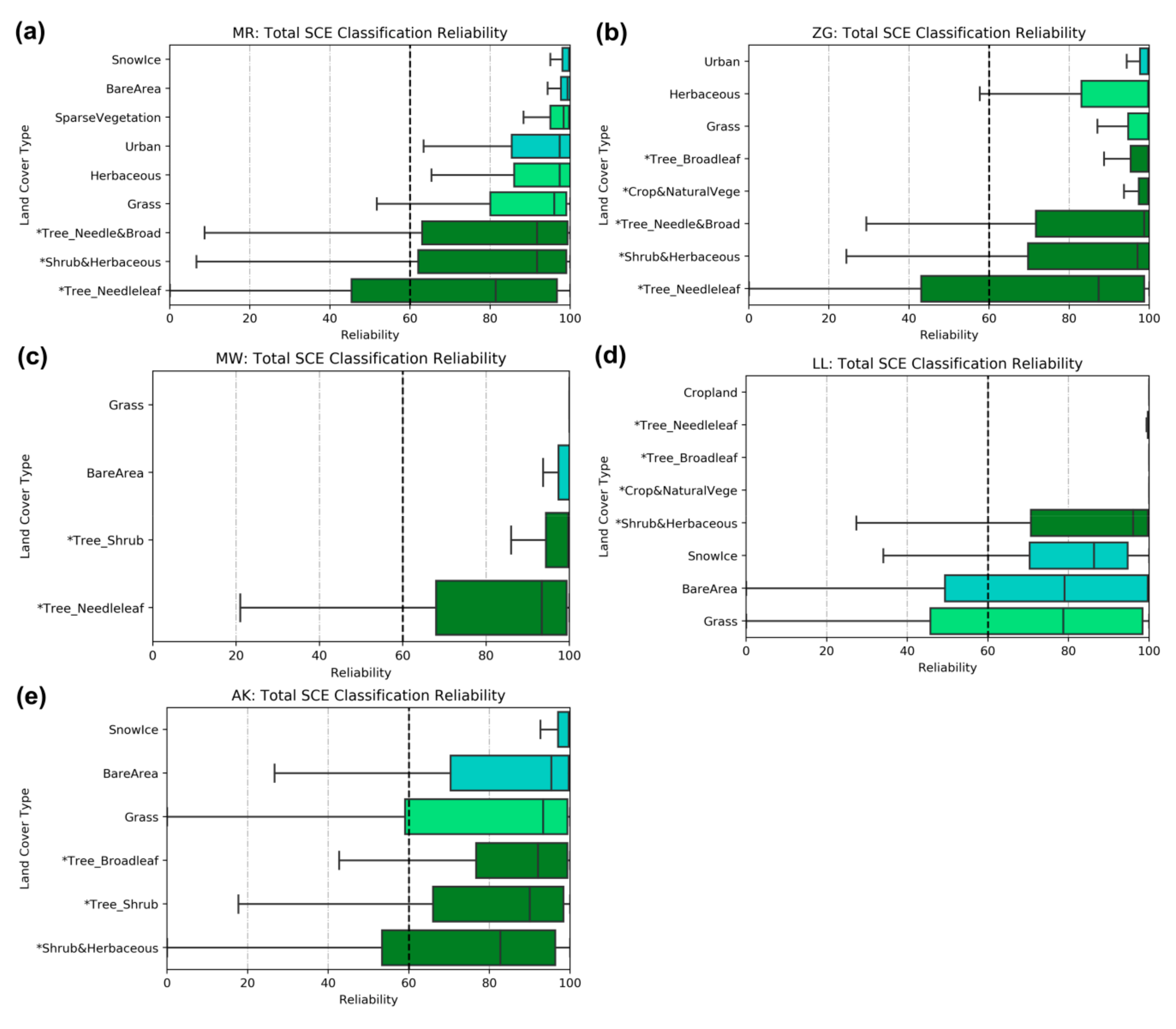
5.2. The Influence of Different Land Cover (Vegetation) Types on the Classification Reliability
5.3. The Heterogeneity between Multispectral-Based Results/Products for Model Training and Validation
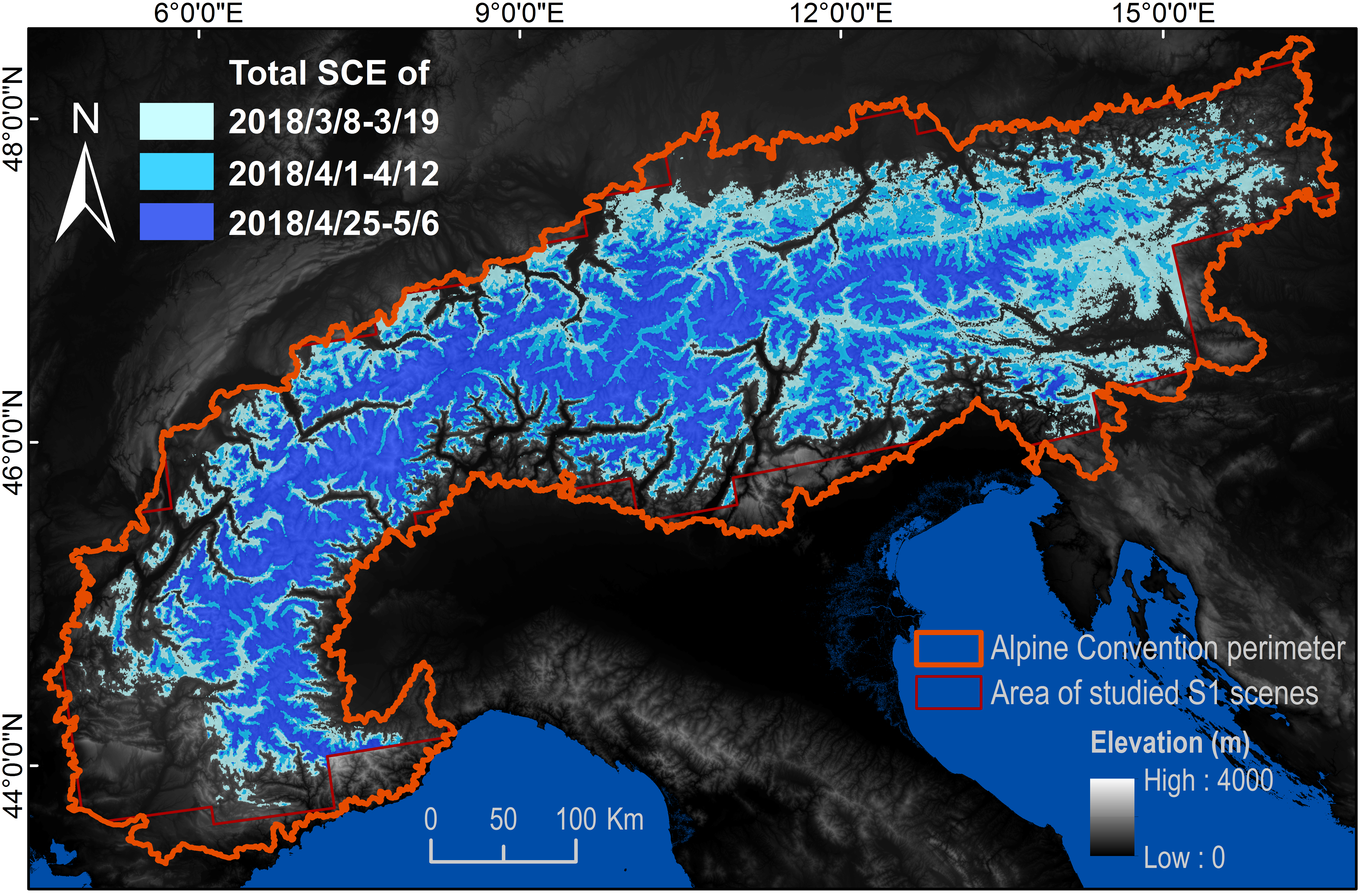
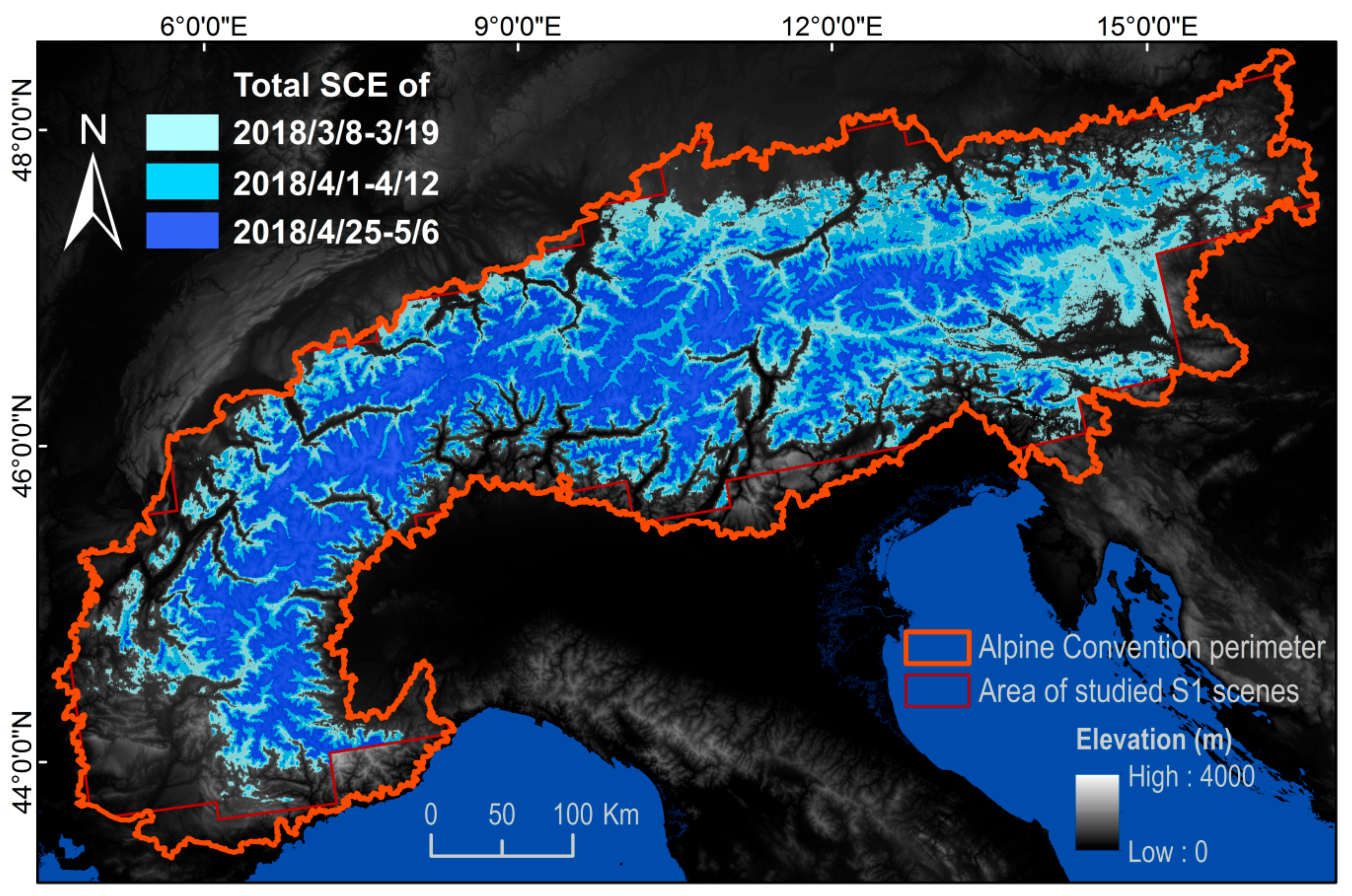
5.4. Applying the Total SCE Detection Approach to a Wider Spatial Scale—The Whole Alps
5.5. Improvements Achieved in This Study and Its Future Potential
6. Conclusions
Author Contributions
Funding
Acknowledgments
Conflicts of Interest
References
- Najafi, M.R.; Zwiers, F.W.; Gillett, N.P. Attribution of the spring snow cover extent decline in the Northern Hemisphere, Eurasia and North America to anthropogenic influence. Clim. Chang. 2016, 136, 71–586. [Google Scholar] [CrossRef]
- Hori, M.; Sugiura, K.; Kobayashi, K.; Aoki, T.; Tanikawa, T.; Kuchiki, K.; Niwano, M.; Enomoto, H. A 38-year (1978–2015) Northern Hemisphere daily snow cover extent product derived using consistent objective criteria from satellite-borne optical sensors. Remote Sens. Environ. 2017, 191, 402–418. [Google Scholar] [CrossRef]
- Pachauri, R.K.; Allen, M.R.; Barros, V.R.; Broome, J.; Cramer, W.; Christ, R.; Church, J.A.; Clarke, L.; Dahe, Q.; Dasgupta, P. Climate Change 2014: Synthesis Report. Contribution of Working Groups I, II and III to the Fifth Assessment Report of the Intergovernmental Panel on Climate Change; IPCC: Geneva, Switzerland, 2014. [Google Scholar]
- Hoegh-Guldberg, O.; Jacob, D.; Taylor, M.; Bindi, M.; Brown, S.; Camilloni, I.; Diedhiou, A.; Djalante, R.; Ebi, K.; Engelbrecht, F. Impacts of 1.5 ºC Global Warming On Natural And Human Systems; International Institute for Applied Systems Analysis (IIASA): Laxenburg, Austria, 2018. [Google Scholar]
- Huss, M.; Bookhagen, B.; Huggel, C.; Jacobsen, D.; Bradley, R.S.; Clague, J.J.; Vuille, M.; Buytaert, W.; Cayan, D.R.; Greenwood, G. Toward mountains without permanent snow and ice. Earth’s Future 2017, 5, 418–435. [Google Scholar] [CrossRef]
- Singh, G.; Venkataraman, G.; Yamaguchi, Y.; Park, S.E. Capability Assessment of Fully Polarimetric ALOS–PALSAR Data for Discriminating Wet Snow From Other Scattering Types in Mountainous Regions. IEEE Trans. Geosci. Remote Sens. 2014, 52, 1177–1196. [Google Scholar] [CrossRef]
- Schöber, J.; Schneider, K.; Helfricht, K.; Schattan, P.; Achleitner, S.; Schöberl, F.; Kirnbauer, R. Snow cover characteristics in a glacierized catchment in the Tyrolean Alps-Improved spatially distributed modelling by usage of Lidar data. J. Hydrol. 2014, 519, 3492–3510. [Google Scholar] [CrossRef]
- Barnett, T.P.; Adam, J.C.; Lettenmaier, D.P. Potential impacts of a warming climate on water availability in snow-dominated regions. Nature 2005, 438, 303. [Google Scholar] [CrossRef] [PubMed]
- Beniston, M.; Farinotti, D.; Stoffel, M.; Andreassen, L.M.; Coppola, E.; Eckert, N.; Fantini, A.; Giacona, F.; Hauck, C.; Huss, M. The European mountain cryosphere: A review of its current state, trends, and future challenges. Cryosphere 2018, 12, 759. [Google Scholar] [CrossRef]
- Pogliotti, P.; Guglielmin, M.; Cremonese, E.; di Cella, U.M.; Filippa, G.; Pellet, C.; Hauck, C. Warming permafrost and active layer variability at Cime Bianche, Western European Alps. Cryosphere 2015, 9, 647–661. [Google Scholar] [CrossRef] [Green Version]
- Yang, Y.; Leppäranta, M.; Cheng, B.; Li, Z. Numerical modelling of snow and ice thicknesses in Lake Vanajavesi, Finland. Tellus A Dyn. Meteorol. Oceanogr. 2012, 64, 17202. [Google Scholar] [CrossRef]
- Riggs, G.A.; Hall, D.K. MODIS Snow Products Collection 6 User Guide; National Snow and Ice Data Center: Boulder, CO, USA, 2015. [Google Scholar]
- Solberg, R.; Wangensteen, B.; Metsämäki, S.; Nagler, T.; Sandner, R.; Rott, H.; Wiesmann, A.; Luojus, K.; Kangwa, M.; Pulliainen, J. GlobSnow Snow Extent Product Guide Product Version 1.0; European Space Angency: Helsinki, Finland, 2010. [Google Scholar]
- Bartsch, A.; Jansa, J.; Schöner, M.; Wagner, W. Monitoring of Spring Snowmelt with Envisat ASAR WS in the Eastern Alps by Combination of Ascending and Descending Orbits; Vienna University of Technology: Vienna, Austria, 2007. [Google Scholar]
- Macander, M.J.; Swingley, C.S.; Joly, K.; Raynolds, M.K. Landsat-based snow persistence map for northwest Alaska. Remote Sens. Environ. 2015, 163, 23–31. [Google Scholar] [CrossRef]
- Tsai, Y.-L.S.; Dietz, A.; Oppelt, N.; Kuenzer, C. Remote Sensing of Snow Cover Using Spaceborne SAR: A Review. Remote Sens. 2019, 11, 1456. [Google Scholar] [CrossRef]
- Nagler, T.; Rott, H. Retrieval of wet snow by means of multitemporal SAR data. IEEE Trans. Geosci. Remote Sens. 2000, 38, 754–765. [Google Scholar] [CrossRef]
- Tsai, Y.L.S.; Dietz, A.; Oppelt, N.; Kuenzer, C. Wet and Dry Snow Detection Using Sentinel-1 SAR Data for Mountainous Areas with a Machine Learning Technique. Remote Sens. 2019, 11, 895. [Google Scholar] [CrossRef]
- Snehmani, M.K.S.; Gupta, R.D.; Bhardwaj, A.; Joshi, P.K. Remote sensing of mountain snow using active microwave sensors: A review. Geocart. Intern. 2015, 30, 1–27. [Google Scholar] [CrossRef]
- Cloude, S.R.; Pottier, E. A review of target decomposition theorems in radar polarimetry. IEEE Trans. Geosci. Remote Sens. 1996, 34, 498–518. [Google Scholar] [CrossRef]
- Huang, L.; Li, Z.; Tian, B.S.; Chen, Q.; Liu, J.L.; Zhang, R. Classification and snow line detection for glacial areas using the polarimetric SAR image. Remote Sens. Environ. 2011, 115, 1721–1732. [Google Scholar] [CrossRef]
- Longepe, N.; Shimada, M.; Allain, S.; Pottier, E. Capabilities of full-polarimetric PALSAR/ALOS for snow extent mapping. In Proceedings of the IGARSS 2008–2008 IEEE International Geoscience and Remote Sensing Symposium, Boston, MA, USA, 7–11 July 2008. [Google Scholar]
- He, G.; Feng, X.; Xiao, P.; Xia, Z.; Wang, Z.; Chen, H.; Li, H.; Guo, J. Dry and Wet Snow Cover Mapping in Mountain Areas Using SAR and Optical Remote Sensing Data. IEEE J. Sel. Top. Appl. Earth Obs. Remote Sens. 2017, 10, 2575–2588. [Google Scholar] [CrossRef]
- Pal, M. Random forest classifier for remote sensing classification. Int. J. Remote Sens. 2005, 26, 217–222. [Google Scholar] [CrossRef]
- Adam, E.; Mutanga, O.; Odindi, J.; Abdel-Rahman, E.M. Land-use/cover classification in a heterogeneous coastal landscape using RapidEye imagery: Evaluating the performance of random forest and support vector machines classifiers. Int. J. Remote Sens. 2014, 35, 3440–3458. [Google Scholar] [CrossRef]
- Rodriguez-Galiano, V.; Sanchez-Castillo, M.; Chica-Olmo, M.; Chica-Rivas, M. Machine learning predictive models for mineral prospectivity: An evaluation of neural networks, random forest, regression trees and support vector machines. Ore Geol. Rev. 2015, 71, 804–818. [Google Scholar] [CrossRef]
- Luojus, K.P.; Pulliainen, J.T.; Metsämäki, S.J.; Hallikainen, M.T. Snow-Covered Area Estimation Using Satellite Radar Wide-Swath Images. IEEE Trans. Geosci. Remote Sens. 2007, 45, 978–989. [Google Scholar] [CrossRef]
- Dedieu, J.P.; de Farias, G.B.; Castaings, T.; Allain-Bailhache, S.; Pottier, E.; Durand, Y.; Bernier, M. Interpretation of a RADARSAT-2 fully polarimetric time-series for snow cover studies in an Alpine context–first results. Can. J. Remote Sens. 2012, 38, 336–351. [Google Scholar] [CrossRef]
- Hongxing, L.; Lei, W.; Jezek, K.C. Automated delineation of dry and melt snow zones in Antarctica using active and passive microwave observations from space. IEEE Trans. Geosci. Remote Sens. 2006, 44, 2152–2163. [Google Scholar] [CrossRef]
- Zhou, C.; Zheng, L. Mapping Radar Glacier Zones and Dry Snow Line in the Antarctic Peninsula Using Sentinel-1 Images. Remote Sens. 2017, 9, 1171. [Google Scholar] [CrossRef]
- Tedesco, M. Snowmelt detection over the Greenland ice sheet from SSM/I brightness temperature daily variations. Geophys. Res. Lett. 2007, 34, 2. [Google Scholar] [CrossRef]
- Pulliainen, J.T. Investigation on the Backscattering Properties of Finnish Boreal Forests at C-and X-band: A Semi-Empirical Modeling Approach. Ph.D. Thesis, Helsinki University of Technology, Espoo, Finland, 1994. [Google Scholar]
- Pulliainen, J.T.; Heiska, K.; Hyyppa, J.; Hallikainen, M.T. Backscattering properties of boreal forests at the C-and X-bands. IEEE Trans. Geosci. Remote Sens. 1994, 32, 1041–1050. [Google Scholar] [CrossRef]
- Park, S.-E.; Yamaguchi, Y.; Singh, G.; Yamaguchi, S.; Whitaker, A.C. Polarimetric SAR Response of Snow-Covered Area Observed by Multi-Temporal ALOS PALSAR Fully Polarimetric Mode. IEEE Trans. Geosci. Remote Sens. 2014, 52, 329–340. [Google Scholar] [CrossRef]
- Dietz, A.J.; Kuenzer, C.; Dech, S. Global SnowPack: A new set of snow cover parameters for studying status and dynamics of the planetary snow cover extent. Remote Sens. Lett. 2015, 6, 844–853. [Google Scholar] [CrossRef]
- Baret, F.; Weiss, M.; Verger, A.; Smets, B. Atbd For Lai, Fapar And Fcover From Proba-V Products At 300m Resolution (Geov3); INRA: Paris, France, 2016. [Google Scholar]
- Wan, Z.; Hook, S.; Hulley, G. MOD11A1 MODIS/Terra Land Surface Temperature/Emmissivity Daily L3 Global 1 km SIN Grid V006; NASA EOSDIS LP DAAD; NASA: Washington, DC, USA, 2015.
- Wan, Z. Collection-5 Modis Land Surface Temperature Products Users’ Guide; ICESS, University of California: Santa Barbara, CA, USA, 2007. [Google Scholar]
- Mao, K.; Ma, Y.; Tan, X.L.; Shen, X.; Liu, G.; Li, Z.; Chen, J.; Xia, L. Global surface temperature change analysis based on MODIS data in recent twelve years. Adv. Space Res. 2017, 59, 503–512. [Google Scholar] [CrossRef]
- Wan, Z. New refinements and validation of the MODIS land-surface temperature/emissivity products. Remote Sens. Environ. 2008, 112, 59–74. [Google Scholar] [CrossRef]
- Sazonau, V. Implementation and Evaluation of a Random Forest Machine Learning Algorithm; University of Manchester: Manchester, UK, 2012. [Google Scholar]
- Ali, J.; Khan, R.; Ahmad, N.; Maqsood, I. Random forests and decision trees. Int. J. Comput. Sci. Issues (Ijcsi) 2012, 9, 272. [Google Scholar]
- Belgiu, M.; Drăguţ, L. Random forest in remote sensing: A review of applications and future directions. Isprs J. Photogramm. Remote Sens. 2016, 114, 24–31. [Google Scholar] [CrossRef]
- Lewis, D.D.; Gale, W.A. A sequential algorithm for training text classifiers. In Proceedings of the 17th Annual International ACM SIGIR Conference on Research and Development in Information Retrieval, Dublin, Ireland, 3–6 July 1994. [Google Scholar]
- Fawcett, T. An introduction to ROC analysis. Pattern Recognit. Lett. 2006, 27, 861–874. [Google Scholar] [CrossRef]
- Sokolova, M.; Japkowicz, N.; Szpakowicz, S. Beyond accuracy, F-score and ROC: A family of discriminant measures for performance evaluation. In Proceedings of the Australasian Joint Conference on Artificial Intelligence, Hobart, Australia, 4–8 December 2006. [Google Scholar]
- Ferri, C.; Hernández-Orallo, J.; Modroiu, R. An experimental comparison of performance measures for classification. Pattern Recognition Lett. 2009, 30, 27–38. [Google Scholar] [CrossRef]
- Jagt, B.J.V.; Durand, M.T.; Margulis, S.A.; Kim, E.J.; Molotch, N.P. On the characterization of vegetation transmissivity using LAI for application in passive microwave remote sensing of snowpack. Remote Sens. Environ. 2015, 156, 310–321. [Google Scholar] [CrossRef]
- Strobl, C.; Boulesteix, A.L.; Kneib, T.; Augustin, T.; Zeileis, A. Conditional variable importance for random forests. BMC Bioinform. 2008, 9, 307. [Google Scholar] [CrossRef] [PubMed]
- Strobl, C.; Boulesteix, A.L.; Zeileis, A.; Hothorn, T. Bias in random forest variable importance measures: Illustrations, sources and a solution. BMC Bioinform. 2007, 8, 25. [Google Scholar] [CrossRef]
- Luojus, K.P.; Pulliainen, J.T.; Metsämäki, S.J.; Hallikainen, M.T. Accuracy assessment of SAR data-based snow-covered area estimation method. IEEE Trans. Geosci. Remote Sens. 2006, 44, 277–287. [Google Scholar] [CrossRef]
- Qiu, S.; He, B.; Zhu, Z.; Liao, Z.; Quan, X. Improving Fmask cloud and cloud shadow detection in mountainous area for Landsats 4–8 images. Remote Sens. Environ. 2017, 199, 107–119. [Google Scholar] [CrossRef]
- Tank, A.K.; Wijngaard, J.; Können, G.; Böhm, R.; Demarée, G.; Gocheva, A.; Mileta, M.; Pashiardis, S.; Hejkrlik, L.; Kern-Hansen, C. Daily dataset of 20th-century surface air temperature and precipitation series for the European Climate Assessment. Int. J. Clim. 2002, 22, 1441–1453. [Google Scholar] [CrossRef]
- Tsai, Y.; Lin, S.; Kim, J. Tracking Greenland Russell Glacier Movements Using Pixel-offset Method. J. Photogramm. Remote Sens. 2018, 23, 173–189. [Google Scholar]
- Malnes, E.; Storvold, R.; Lauknes, I.; Pettinato, S. Multi-polarisation measurements of snow signatures with air-and satelliteborne SAR. Earsel Eproceedings 2006, 5, 111. [Google Scholar]
- Pettinato, S.; Malnes, E.; Haarpaintner, J. Snow cover maps with satellite borne SAR: A new approach in harmony with fractional optical SCA retrieval algorithms. In Proceedings of the IEEE International Geoscience and Remote Sensing Symposium, Denver, CO, USA, 31 July–4 August 2006. [Google Scholar]
- Storvold, R.; Malnes, E.; Larsen, Y.; Høgda, K.; Hamran, S.; Mueller, K.; Langley, K. SAR remote sensing of snow parameters in norwegian areas—Current status and future perspective. J. Electromagn. Waves Appl. 2006, 20, 1751–1759. [Google Scholar] [CrossRef]
- Löw, A.; Ludwig, R.; Mauser, W. Land use dependent snow cover retrieval using multitemporal, multisensoral SAR-images to drive operational flood forecasting models. In Proceedings of the of EARSeL-LISSIG-Workshop Observing our Cryosphere from Space, Bern, Switzerland, 11–13 March 2002. [Google Scholar]
- Schellenberger, T.; Ventura, B.; Zebisch, M.; Notarnicola, C. Wet Snow Cover Mapping Algorithm Based on Multitemporal COSMO-SkyMed X-Band SAR Images. IEEE J. Sel. Top. Appl. Earth Obs. Remote Sens. 2012, 5, 1045–1053. [Google Scholar] [CrossRef]
- Duguay, Y.; Bernier, M. The use of RADARSAT-2 and TerraSAR-X data for the evaluation of snow characteristics in subarctic regions. In Proceedings of the 2012 IEEE International Geoscience and Remote Sensing Symposium (IGARSS), Munich, Germany, 22–27 July 2012. [Google Scholar]
- Key, J.; Drinkwater, M.; Ukita, J. IGOS cryosphere theme report. WMO/TD 2007, 1405, 100. [Google Scholar]
- Torres, R.; Lokas, S.; di Cosimo, G.; Geudtner, D.; Bibby, D. Sentinel 1 evolution: Sentinel-1C and-1D models. In Proceedings of the 2017 IEEE International Geoscience and Remote Sensing Symposium (IGARSS), Fort Worth, TX, USA, 23–28 July 2017. [Google Scholar]


| Testing Sites | 1 (MR) | 2 (ZG) | 3 (MW) | 4 (LL) | 6 (AK) |
|---|---|---|---|---|---|
| Continent | Europe | Europe | North America | Asia | Australia |
| Mountain Range (Country) | Alps (Switzerland) | Alps (Germany) | Sierra Nevada (U.S.A.) | Himalaya (Nepal) | Southern Alps (New Zealand) |
| Highest Peaks (Height) | Monte Rosa (4634 m) | Zugspitze (2962 m) | Mount Whitney (4421 m) | Langtang Lirung (7234 m) | Aoraki/Mount Cook (3724 m) |
| Region | Training Set (First Hydrological Year) * Reference Image | Validation Set (Second Hydrological Year) | |
|---|---|---|---|
| Month1 (Month not Included in Training Set) | Month2 (Month Included in Training Set) | ||
| Test Site 1: Monte Rosa (MR) (Sentinel-1A, Ascending, relative orbit number: 88) (Landsat-7/8, path: 195, row: 28) | 17–29 November 2016 | 24 March– 5 April 2018 (L7: 23 March) | 23 May– 4 June 2018 (L8: 18 May) |
| 9–21 February 2017 | |||
| 16–28 May 2017 | |||
| * 8 August 2017 | |||
| Test Site 2: Zugspitze (ZG) (Sentinel-1A, Ascending, relative orbit number: 117) (Landsat-7, path: 193, row: 27) (Sentinel-2, tile number: T32TPT) | 7–19 November 2016 | 26 March– 7 April 2018 (L7: 25 March) | 13–25 May 2018 (S2: 7 May) |
| 23 February– 7 March 2017 | |||
| 18–30 May 2017 | |||
| * 10 August 2017 | |||
| Test Site 3: Mount Whitney (MW) (Sentinel-1A, Ascending, relative orbit number: 144) (Landsat-7, path: 41, row: 35) | 25 February– 9 March 2017 | 16–28 March 2018 (L7: 16 March) | 3–15 May 2018 (L7: 3 May) |
| 2–14 April 2017 | |||
| 8–20 May 2017 | |||
| * 12 August 2017 | |||
| Test Site 4: Landtang Lirung (LL) (Sentinel-1A, Ascending, relative orbit number: 85) (Landsat-7, path: 141, row: 40) | 9–21 February 2017 | 12–24 March 2018 (L7: 13 March) | 11–23 May 2018 (L7: 16 May) |
| 10–22 April 2017 | |||
| 16–28 May 2017 | |||
| * 8 August 2017 | |||
| Test Site 5: Aoraki (AK) (Sentinel-1B, Ascending, relative orbit number: 23) (Landsat-7/8, path: 75, row: 90) | 6–18 May 2017 | 30 June– 12 July 2018 (L8: 26 June) | 1–13 May 2018 (L7: 1 May) |
| 10–22 August 2017 | |||
| 21 October– 2 November 2017 | |||
| * 6 February 2018 | |||
| Input Variable | Data Category | Source | Spatial Resolution | Temporal Resolution |
|---|---|---|---|---|
| Total SCE | Ground truth | Global SnowPack | 500 m | Daily |
| Land cover | Land cover label | European Space Agency (ESA) Climate Change Initiative (CCI) land cover | 300 m | Annually |
| Backscattering coefficient | SAR observation | SAR image processing (Sentinel-1) | 5 × 20 m | 12 days |
| Interferometric SAR (InSAR) coherence | ||||
| Polarimetric SAR (PolSAR) entropy | ||||
| PolSAR anisotropy | ||||
| PolSAR angle | ||||
| Elevation | Topographical factor | SRTM digital elevation model (DEM) | 90 m | N/A |
| Slope | ||||
| Aspect | ||||
| Curvature | ||||
| Leaf area index | Vegetation index | Copernicus Global Land Service (PROBA-V based) | 300 m | 10 days |
| Fractional vegetation cover | ||||
| Land surface temperature | Temperature | MOD/MYD11A2 (MODIS based) | 1000 m | 8 days |
© 2019 by the authors. Licensee MDPI, Basel, Switzerland. This article is an open access article distributed under the terms and conditions of the Creative Commons Attribution (CC BY) license (http://creativecommons.org/licenses/by/4.0/).
Share and Cite
Tsai, Y.-L.S.; Dietz, A.; Oppelt, N.; Kuenzer, C. A Combination of PROBA-V/MODIS-Based Products with Sentinel-1 SAR Data for Detecting Wet and Dry Snow Cover in Mountainous Areas. Remote Sens. 2019, 11, 1904. https://doi.org/10.3390/rs11161904
Tsai Y-LS, Dietz A, Oppelt N, Kuenzer C. A Combination of PROBA-V/MODIS-Based Products with Sentinel-1 SAR Data for Detecting Wet and Dry Snow Cover in Mountainous Areas. Remote Sensing. 2019; 11(16):1904. https://doi.org/10.3390/rs11161904
Chicago/Turabian StyleTsai, Ya-Lun S., Andreas Dietz, Natascha Oppelt, and Claudia Kuenzer. 2019. "A Combination of PROBA-V/MODIS-Based Products with Sentinel-1 SAR Data for Detecting Wet and Dry Snow Cover in Mountainous Areas" Remote Sensing 11, no. 16: 1904. https://doi.org/10.3390/rs11161904