Using Forest Inventory Data with Landsat 8 Imagery to Map Longleaf Pine Forest Characteristics in Georgia, USA


1
Rocky Mountain Research Station, U.S. Forest Service, Missoula, MT 59801, USA
2
W.A. Franke College of Forestry and Conservation, University of Montana, Missoula, MT 59812, USA
3
North Fork Analytics, LLC. Onsite contractor with Rocky Mountain Research Station, U.S. Forest Service, Missoula, MT 59801, USA
*
Author to whom correspondence should be addressed.
Remote Sens. 2019, 11(15), 1803; https://doi.org/10.3390/rs11151803
Submission received: 22 May 2019
/
Revised: 19 July 2019
/
Accepted: 26 July 2019
/
Published: 1 August 2019
(This article belongs to the Special Issue Forest Health Monitoring)
Abstract
:This study improved on previous efforts to map longleaf pine (Pinus palustris) over large areas in the southeastern United States of America by developing new methods that integrate forest inventory data, aerial photography and Landsat 8 imagery to model forest characteristics. Spatial, statistical and machine learning algorithms were used to relate United States Forest Service Forest Inventory and Analysis (FIA) field plot data to relatively normalized Landsat 8 imagery based texture. Modeling algorithms employed include softmax neural networks and multiple hurdle models that combine softmax neural network predictions with linear regression models to estimate key forest characteristics across 2.3 million ha in Georgia, USA. Forest metrics include forest type, basal area and stand density. Results show strong relationships between Landsat 8 imagery based texture and field data (map accuracy > 0.80; square root basal area per ha residual standard errors < 1; natural log transformed trees per ha < 1.081). Model estimates depicting spatially explicit, fine resolution raster surfaces of forest characteristics for multiple coniferous and deciduous species across the study area were created and made available to the public in an online raster database. These products can be integrated with existing tabular, vector and raster databases already being used to guide longleaf pine conservation and restoration in the region.

1. Introduction
Longleaf pine (Pinus palustris) ecosystems are some of the most critically endangered ecosystems in the world [1]. What remains of these once dominant forests supports many plants and animals and provides refuge for threatened and endangered species [2]. Though the negative ecological impacts of longleaf pine losses are still being studied across the southeastern United States of America (USA), it is clear that these systems provide critical habitat for many species. Widespread concern among public agencies, non-governmental organizations (NGO) and private companies have stimulated restoration efforts and the development of the Range-Wide Conservation Plan for Longleaf Pine, which called for doubling the area of longleaf ecosystems and improving the condition of established longleaf forests by 2024 [3]. By 2014, at least 558,000 ha of longleaf pine had been restored, 445,000 ha had been improved through prescribed burning, 63,000 ha had been established through planting and 30,428 ha had been improved through the removal of invasive species and the opening of the forest canopy [4]. While impressive, early success heavily leveraged expert opinion related to the condition and location of longleaf ecosystems and capitalized on programs previously established to restore longleaf pine. Well-known sites under ownership amenable to investments in conservation and restoration were targeted early. However, information characterizing the location and condition of all forests in addition to longleaf pine forests, across all ownerships, including those unfamiliar to experts, is needed to maintain the pace of restoration and meet the goals of the Range-Wide Conservation Plan.
In 2015, the authors, together with government and NGO partners, began a series of studies aimed at improving the resolution, extent, accuracy and utility of spatial analysis and mapping products available for longleaf pine projects. This work leveraged new statistical methods and novel data structures and algorithms that were initially developed for mapping forest characteristics in the western USA [5,6,7,8]. Image texture metrics and principle components derived from National Agriculture Imagery Program (NAIP) aerial photographic imagery [9] were used with a softmax neural network model to produce probabilistic classification surfaces at 1 m resolution across 11.6 million ha in the southeast USA [10]. Species composition, basal area and stand tree density for pine and hardwood tree species, including longleaf pine, were then estimated at coarser resolution (78 m by 70 m) for the study area using random forest methods, Forest Inventory and Analysis (FIA) inventory plot data [11] and image spectral and texture metrics [12]. Strong relationships between forest characteristics measured in field plots and metrics derived from imagery were found in this investigation and this estimation approach significantly reduced error and improved spatial detail over classical aggregation techniques [12]. Despite clear benefits over traditional techniques of classifying forests and estimating forest characteristics using plot data alone, both studies [10,12] encountered problems with using NAIP imagery. Due to the variation in image acquisition dates and the color balancing technique used to mosaic NAIP images together, resulting raster surfaces had increased estimation error and displayed visual striping along flight paths. Hogland et al. [12] suggested relating plot data and finer resolution NAIP imagery to spatially coarser but temporally finer Landsat 8 imagery to alleviate these negative effects and also highlighted several other potential advantages of using Landsat 8. However, no study to date has used FIA field plots, multi-temporal Landsat imagery and image texture in this manner to spatially quantify key forest characters for longleaf restoration.
The study described here developed and implemented a variety of improvements to previous approaches for a study area that had not been previously mapped using these techniques. The goal of the study was to provide new information and facilitate the expansion of quality longleaf pine habitat across its historic range. In addition to knowing the location and condition of existing longleaf pine habitat, the condition and locations of forested habitat that currently occupies potential longleaf habitat were also mapped to aid in prioritizing restoration efforts. The objectives of this study were to: (1) develop new analytical techniques to map longleaf pine, other forest types and associated forest characteristics efficiently across large landscapes using commonly available imagery and data, (2) demonstrate these methods for a study area with complex land cover and high potential for longleaf pine restoration and (3) disseminate methods and tools to facilitate similar analyses and resulting datasets to inform longleaf restoration efforts. An important outcome was to solve problems encountered in previous studies including model extrapolation and the striping phenomenon associated with using NAIP imagery as a predictor variable.
2. Materials and Methods
2.1. Study Area
The Fort Stewart/Altamaha River Longleaf Pine Significant Geographic Area (referred to hereafter as the “Fort Stewart SGA,” Figure 1) is an area of particular conservation interest designated through America’s Longleaf Restoration Initiative [13]. This SGA covers a large portion of Georgia, is located within the heart of the historic distribution of longleaf pine and includes both publicly and privately owned lands. The area is about 2 million ha (5 million ac) and includes the Fort Stewart Military Reservation in the northeast corner and conservation lands along the Altamaha River and Altamaha Conservation Corridor [14]. Unique features include diverse longleaf pine sandhills and flatwoods with associated wetlands that are typically maintained by frequent fire, which is an important restoration tool in this habitat [14]. The area is home to several animal species of high conservation concern, including the red-cockaded woodpecker (Leuconotopicus borealis), Bachman’s sparrow (Peucaea aestivalis), frosted flatwoods salamander (Ambystoma cingulatum), gopher tortoise (Gopherus polyphemus) and indigo snake (Drymarchon spp.).
2.2. Data
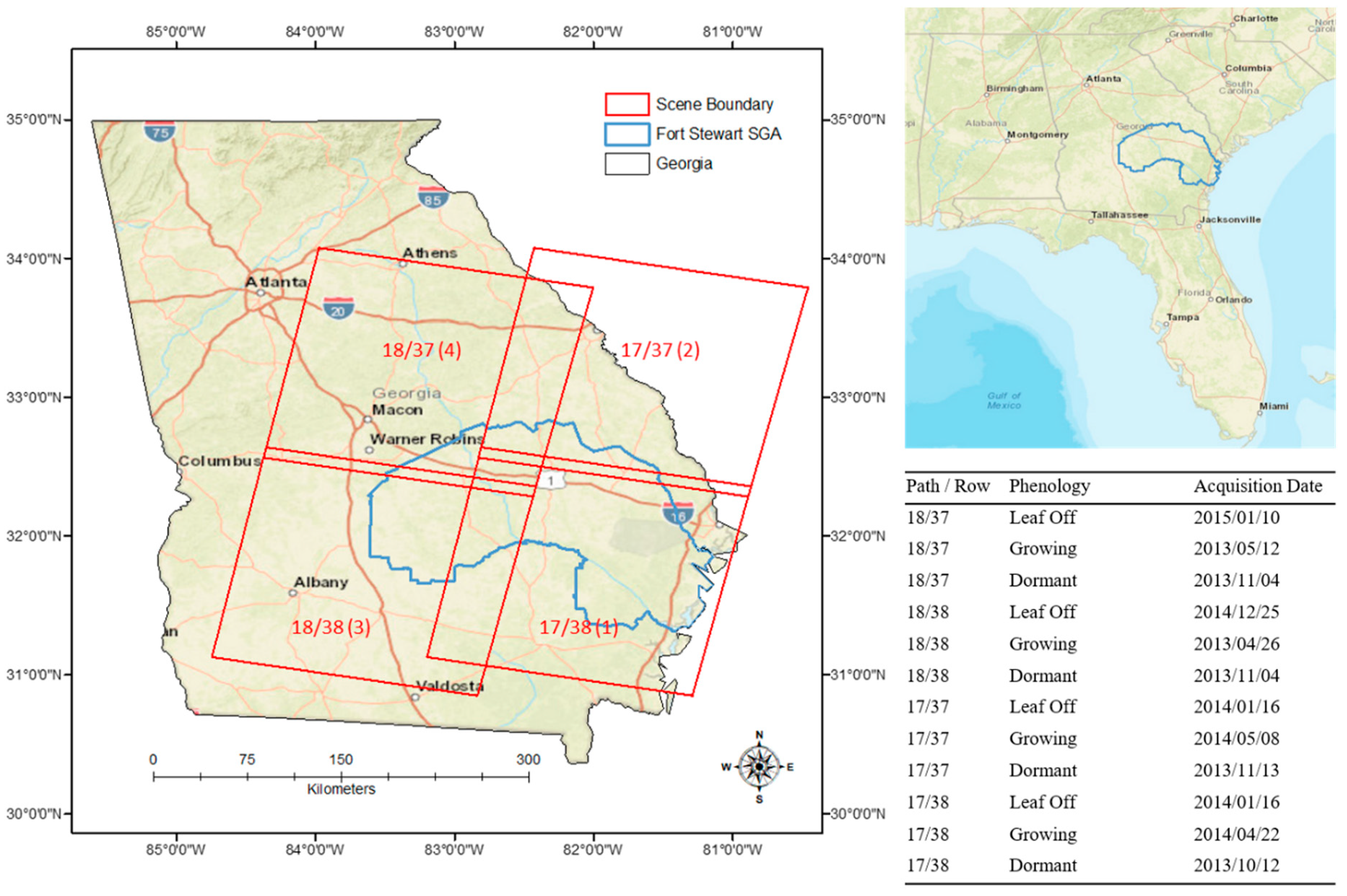
Primary datasets used in this study were FIA field plot data, NAIP imagery and multi-temporal Landsat 8 imagery with level 1 terrain precision (L1TP) correction. FIA data were downloaded from FIA’s DataMart website [15]. The exact spatial locations of FIA plots are kept confidential but were obtained for this study directly from FIA following the procedures described on FIA’s spatial data request webpage [16]. NAIP images were downloaded from the United States Geological Survey (USGS) FTP site [17]. Landsat images were downloaded from the USGS Earth Explorer website (Figure 1) [18]. In total 1033 FIA plots, 972 NAIP images and 12 Landsat images were downloaded for the project.
While many other datasets were initially evaluated as potential predictors of forest characteristics (including soils, digital elevation models (DEM) and ecoregions), these datasets did not provide the coverage, detail and consistency needed to produce SGA-wide estimates of key forest characteristics. Of the datasets that did have the necessary characteristics, NAIP color infrared (CIR) and Landsat 8 imagery were chosen as the primary predictor datasets [9,19]. NAIP is preprocessed to a balanced radiometric scale for each state, is readily available for free, has a fine spatial resolution (1 m), is reacquired every two years and has complete coverage within conterminous USA. Similarly, Landsat 8 imagery has complete coverage across the USA and is also available for free. Landsat 8 imagery, though, has a coarser spatial resolution (30 m) than NAIP but finer temporal resolution (16 days). In addition, Landsat 8 also has a broader spectral range than NAIP.
Due to the fine spatial resolution and associated large storage size of the NAIP imagery, we built an automated download tool called “Download Data” that systematically selected and downloaded each NAIP image tile for a defined area of interest using a file transfer protocol (FTP) website, tiled feature class and an area of extent [9,17,20] (Table A1). In total, 972 NAIP images were downloaded and stored locally. Once downloaded, these images were assembled into a mosaic raster dataset [21] for the Fort Stewart SGA and prepared for analysis.
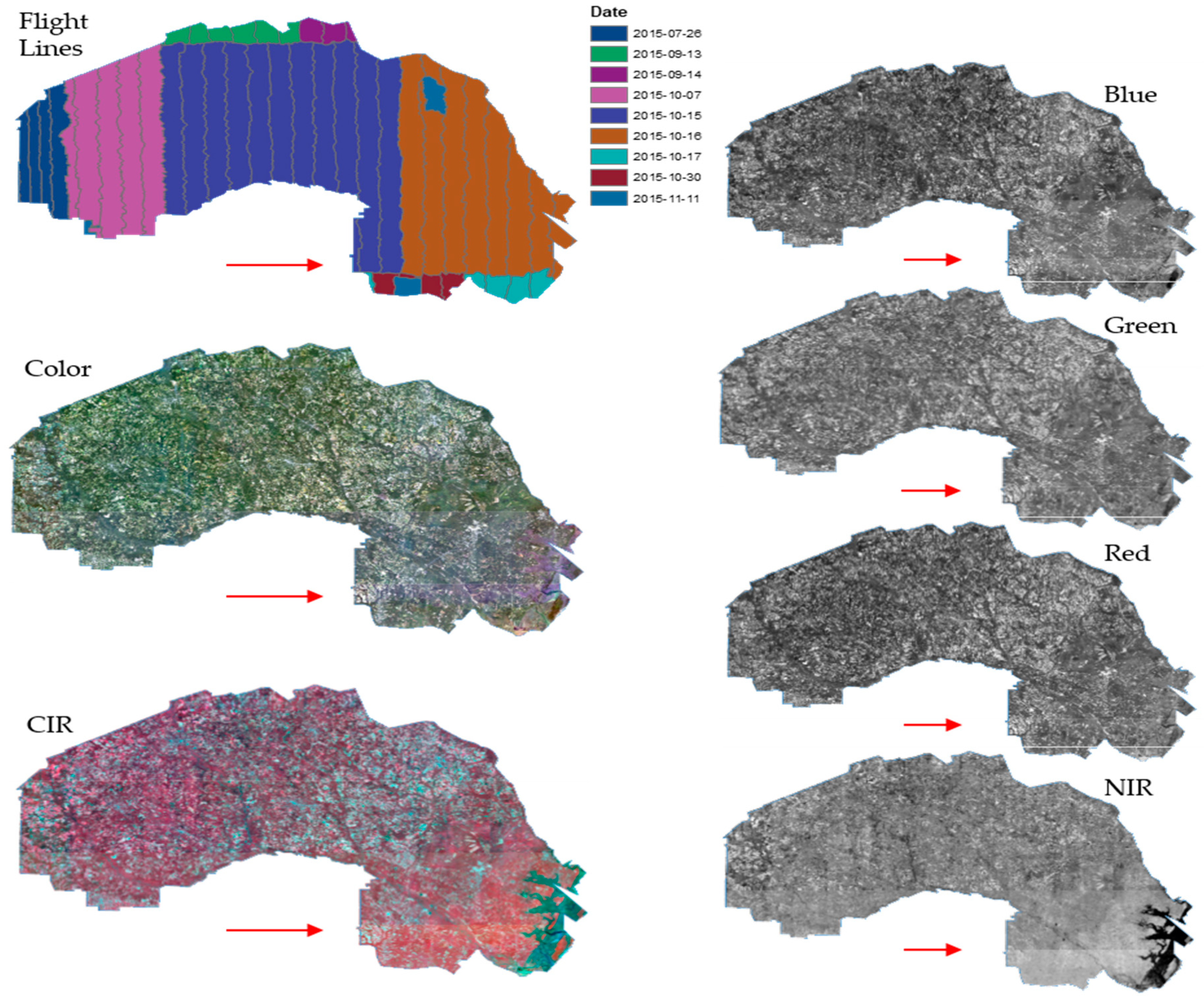
To acquire flight line data associated with the NAIP imagery, we built a set of routines encapsulated within a graphical user interface called “Map Services Download” that opens map services, queries records from those services and builds new locally stored vector datasets depicting the information within those services [22]. Using the “Map Services Download” tool we recreated NAIP flight line datasets found on Aerial Photography Field Office (APFO) map service (https://gis.apfo.usda.gov/arcgis/services). NAIP imagery within SGAs was collected from July 2015 to November 2015 and varied by date and time of collection. Though the NAIP program tries to visually minimize the effects of acquiring imagery at various dates and times using a color balancing mosaicking processes [9], significant striping and variation in atmospheric conditions were visible along flight lines in the mosaic raster dataset (Figure 2). This was a substantial source of error identified in the previous longleaf based study [12] and in large part the rationale for evaluating coarser grained imagery such as produced by the Landsat 8 program.
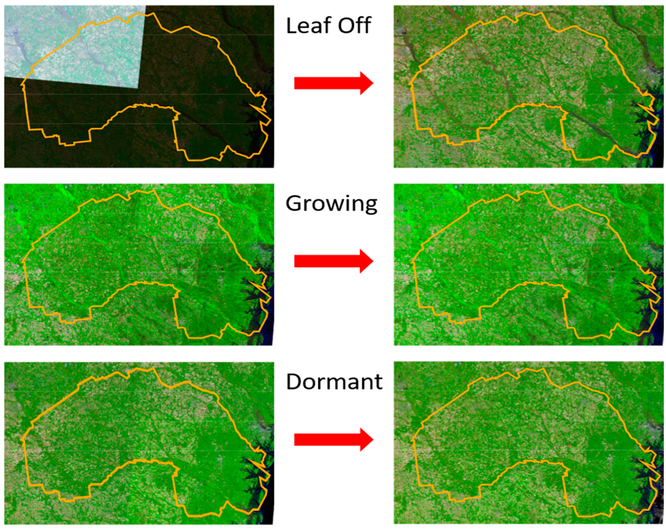
To evaluate the use of Landsat 8 imagery, four adjacent L1TP images were manually selected for each of three phenologies. Phenologies were selected to identify three different periods of growth for overstory trees that vary spectrally and include a winter (Leaf Off), spring (Growing) and fall (Dormant) season. Image acquisition dates were selected to closely coincide with the year of NAIP acquisition and FIA field plot data (Figure 1) while minimizing cloud coverage. Landsat 8 bands one through seven were used for our evaluations. Similar to NAIP image boundaries, Landsat scene boundaries can have substantially different cell values given time and date of acquisition even within a given phenological period. However, different from NAIP, Landsat images are freely available in their native digital number (DN) format and have overlapping regions which can be used to bring images to a common radiometric scale.
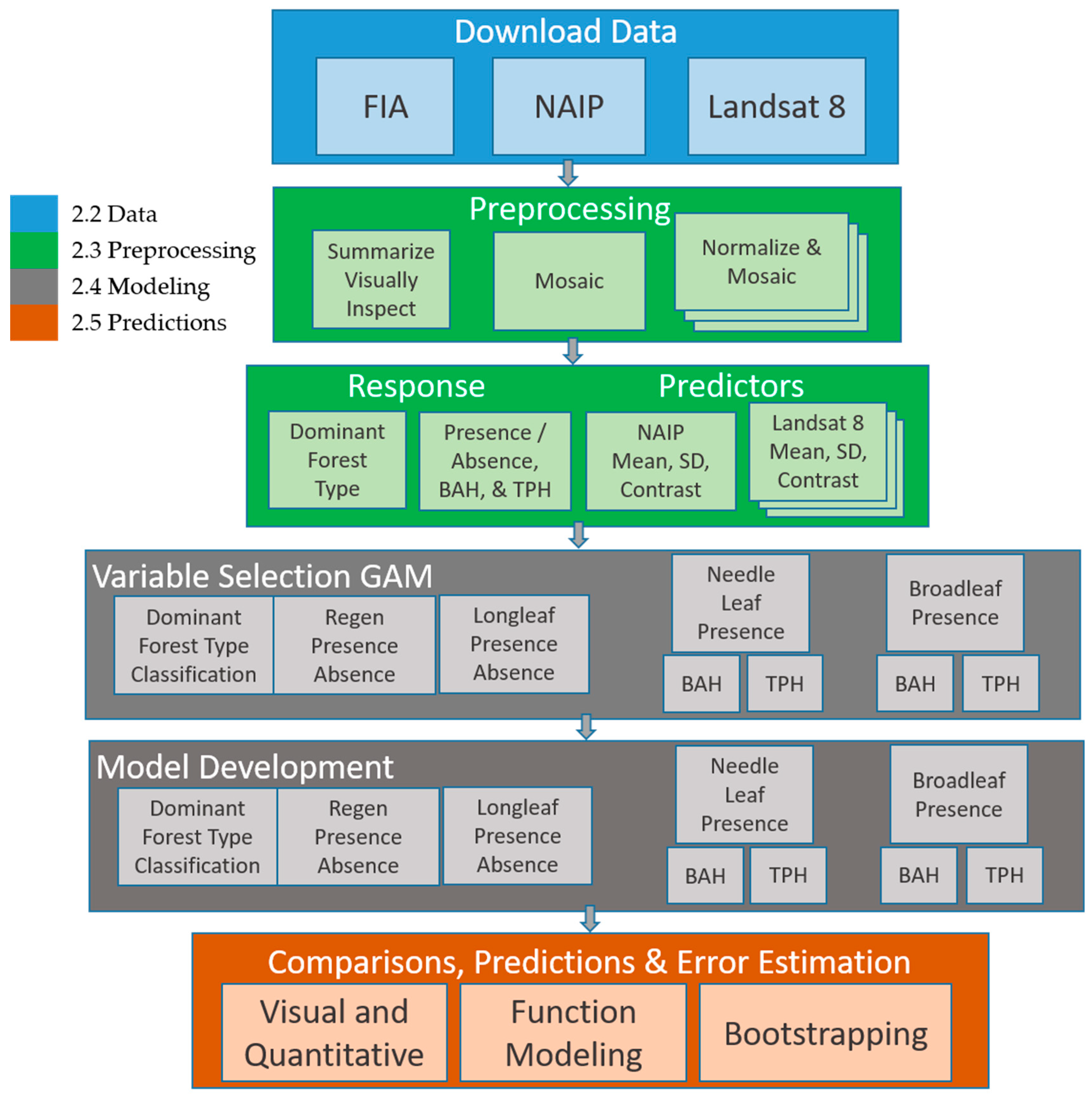
Using these primary datasets, we performed a series of data preprocessing steps (Section 2.3) to summarize, normalize and build response and predictor variables from FIA plot data and NAIP and Landsat 8 imagery. Response and predictor variables were then used to calibrate a suite of predictive models (Section 2.4) which in turn were used to create multiple raster surfaces with estimates of key forest characteristics for longleaf restoration (Section 2.5). Key forest characteristics needed to inform longleaf restoration included: dominant forest cover, needle and broadleaf tree species presence, longleaf pine tree species presence, regeneration areas and basal area (basal area per hectare, BAH) and stand density (trees per hectare, TPH) for broad and needle-leaf tree species. Figure 3 provides a visual overview of the steps used to acquire, transform, make predictions and evaluate estimates of the raster surfaces depicting key forest characteristics.
2.3. Preprocessing
To facilitate the tabular, spatial, statistical, machine learning and geographic information system (GIS) analyses performed in this study, we developed many new tools that take advantage of Function Modeling [22] and parallel processing (Table A1). The underlying concept behind Function Modeling is delayed reading, which postpones processing data until absolutely necessary and can significantly decrease processing time and the storage of raster based analyses [22]. These newly developed tools build on our previous work [5,20,22,23], integrate seamlessly within ESRI’s GIS as a toolbar add-in (RMRS Raster Utility toolbar), are available for free download [20] and provide a wide range of analytical functionality that is not otherwise available within the research or practitioner communities.
Using the “Summarize FIA Data” tool within the RMRS Raster Utility toolbar (Table A1), we summarized FIA tabular tree data by species group (Table A2), FIA Status Code and tree size [24] and appended those summaries to the corresponding plot locations. Tree size groupings of FIA data were made according to tree diameter at breast height (DBH, diameter 1.37 m above the ground) in three groups: less than 2.54 cm, 2.54 cm to 12.7 cm and equal to or greater than 12.7 cm. BAH and TPH were then further split into needle-leaf and broadleaf tree species groups (Table A2). In the FIA protocol, seedlings and trees less than 12.7 cm DBH are sampled less intensively than larger trees. Plots for trees greater than or equal to 12.7 cm have a subplot radius of 7.32 m while trees less than 12.7 have a subplot radius of only 2.07 m. To account for measuring different subplot areas the “Summarize FIA Data” tool uses expansion factors to bring all plot measurements to appropriate area estimates (e.g., trees per hectare) [24].
Confidential exact plot locations were acquired from the FIA using established protocols [16]. Of the 1033 FIA plots downloaded and summarized, 271 plots were removed because they had a measurement year before 2011. In addition, for quality assurance a visual inspection of FIA plots was performed in a GIS by comparing summarized TPH estimates to NAIP imagery. For locations where plot summaries clearly differed from what was visible in the imagery (e.g., a field plot indicating TPH where the imagery showed an open field with no trees present) a dominant forest type (i.e., needle-leaf, broadleaf or non-forested) was determined and that record was flagged for removal from presence/absence and BAH and TPH components of the analyses (Table 1). Discrepancies between plot summaries and what is visibly present in the imagery can occur for multiple reasons but most commonly was due to some management action, such as a timber harvest, occurring between the dates of plot measurement and imagery acquisition. In total, 762 FIA plots were available for modeling dominant forest cover, 682 plots were available for modeling presence and absence, 530 plots were available for modeling needle-leaf BAH and TPH and 569 plots were available for modeling broadleaf BAH and TPH.
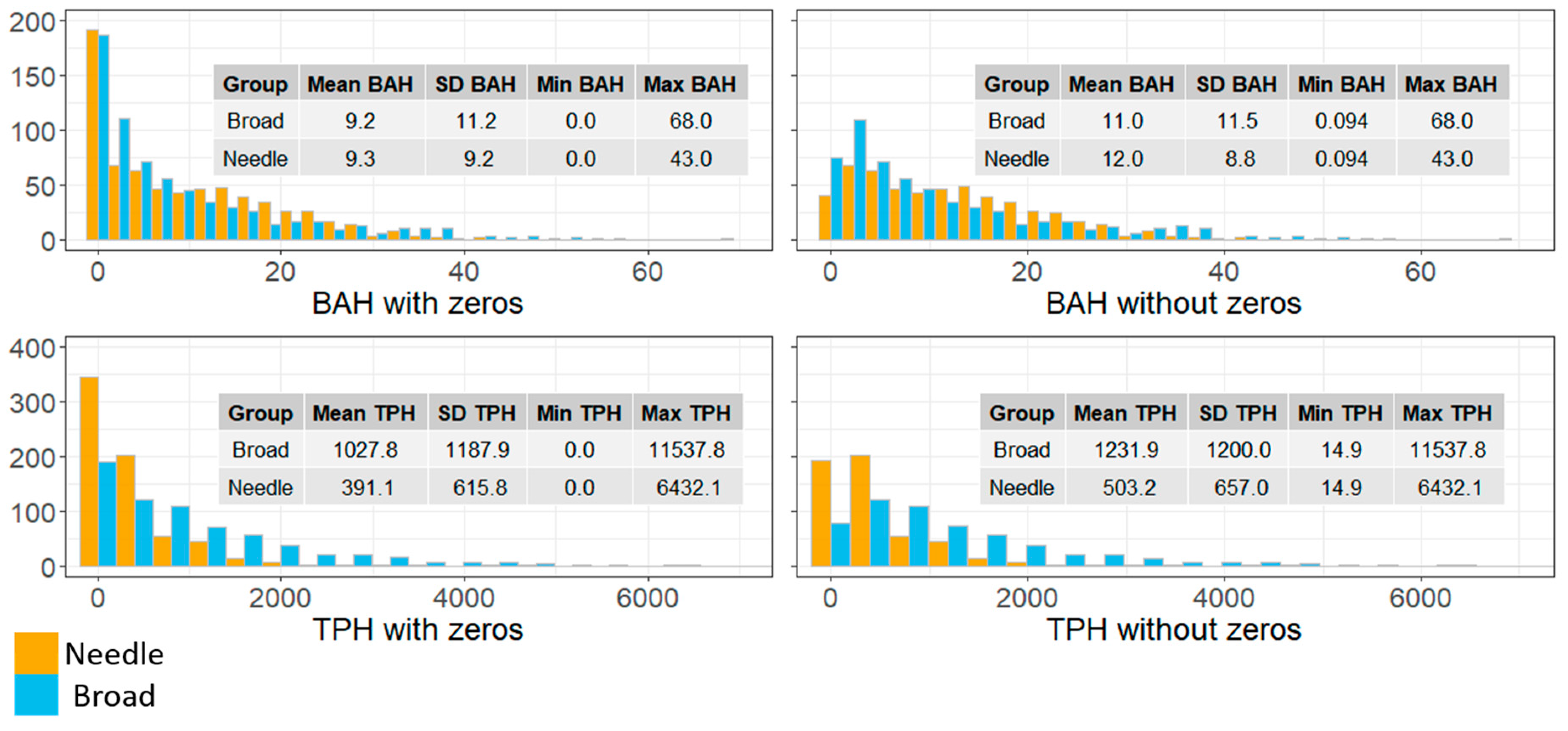
In addition to continuous BAH and TPH response variables for needle-leaf (N_BAH and N_TPH) and broadleaf (B_BAH and B_TPH) species groupings, categorical response variables depicting various aspects of the forest were created from FIA plot summaries. Dominant forest type (DomType), areas composed of primarily regeneration plots (Regen), longleaf pine presence and absence (L_Leaf), needle-leaf tree species presence and absence (N_Leaf) and broadleaf tree species presence and absence (B_Leaf) were identified and labeled using various queries of species, BAH and TPH (Table 1). Due to plots falling in agricultural, urban or harvested areas within the Fort Stewart SGA, there were numerous instances where no trees larger than 12.7 cm in DBH were tallied. While those instances and locations can be identified visually within the imagery and quantitatively within the data (i.e., B_Leaf and L_Leaf variables), without taking into consideration non-forested areas when calibrating BAH and TPH models, estimates could potentially be conflated by an excess number of zeros (Figure 4).
NAIP imagery was not additionally preprocessed after download. In its publicly available form, NAIP imagery comes as a preprocessed mosaic that uses seamlines and a color balancing routine to visually smooth image boundaries [9]. Unfortunately, the unprocessed source images to which the color balancing and mosaicking routines are applied are not readily available, thereby limiting the preprocessing techniques that could be used to bring adjacent NAIP images to a common relative radiometric scale. While useful in its publicly available form, NAIP image mosaics are not normalized and image boundaries are visually apparent within the mosaic (Figure 2).
Landsat 8 imagery was preprocessed. In contrast to NAIP, source data with overlapping boundaries for Landsat 8 imagery are readily available and a variety of methods have been developed and used to normalize Landsat imagery [25,26,27]. While significant improvements have been made with regards to bringing images to a common surface reflectance [28], scene boundaries are often visible among adjacent images acquired during the same phenology but at different dates and times (Figure A1). To address discrepancies in spectral values among scenes we employed a relative normalization technique called aggregate no-change regression (ANR). In previous work, Hogland [29] developed and evaluated ANR using Landsat Enhanced Thematic Mapper Plus imagery. His findings indicate that ANR significantly improved bringing images to a common radiometric scale over other common absolute and relative normalization routines including procedures used to convert DN values to surface reflectance. Based on that work, we operationalized ANR and integrated it into the RMRS Raster Utility toolbar [20] (Table A1).
At its core, ANR extends the concepts of automatic scattergram-controlled regression [30] by applying an area slicing algorithm to identify no-change pixels and then spatially aggregating pixel values to minimize the effect of geo-rectification errors. Aggregated values of defined no change pixels for the overlapping areas of a reference image and a subject image are then regressed against one another on a band basis. Regression coefficients are then applied to the subject image to bring reference and subject images to a common radiometric scale. For Landsat 8 images representing Leaf off, Growing and Dormant phenologies, we were able to use ANR to bring images within a given phenology to a common relative radiometric scale (Figure 5 and Figure A2). Reference images for each Landsat 8 phenology came from path/row 17/38. In instances when substantial land use or land cover change had occurred due to differences in image acquisition dates (e.g., changes in agricultural fields), manually defined spatial masks were used to remove changed pixels from the ANR procedure. Slicing algorithm change percentages used in the ANR process ranged from 20 to 40%.
Preprocessing also included analysis of image texture. After ANR image normalization was completed for the Landsat 8 images, we generated first and second order texture raster surfaces [31]. Texture metrics for NAIP and normalized Landsat 8 imagery included mean, first order standard deviation and a second order horizontal contrast gray level co-occurrence matrix (GLCM) of each NAIP and Landsat 8 band [22,31]. Using “Focal Analysis” and “GLCM Analysis” tools in the RMRS Raster Utility toolbar, we transformed NAIP imagery into 12 new raster surfaces depicting image texture at the spatial extent of an FIA plot (i.e., a 78 m by 70 m focal window). Similarly, for normalized Landsat 8 images we created 63 texture surfaces (3 texture metrics for each of 7 bands and for each of 3 different phenologies) at the spatial extent covering the area of an FIA plot, which in the case of Landsat 8 is a 3 cell by 3 cell (90 m × 90 m) moving window. These raster surfaces were used as potential predictor variables in our predictive modeling.
To relate FIA field data response variables (e.g., BAH and TPH) to NAIP and normalized Landsat 8 potential texture variables, we used the “Sample Values” tool within the RMRS Raster Utility toolbar (Table A1). Using this tool, we extracted the mean, standard deviation and horizontal contrast GLCM texture values derived from NAIP and normalized Landsat 8 imagery (75 potential predictor variables) for the location of each FIA plot and appended those values to the FIA point feature class attribute table. Five categorical (Table 1) and four continuous (Figure 4) response variables and the 75 image-based texture metrics as predictor variables for 762 plot locations constitute our working dataset for model development.
2.4. Modeling
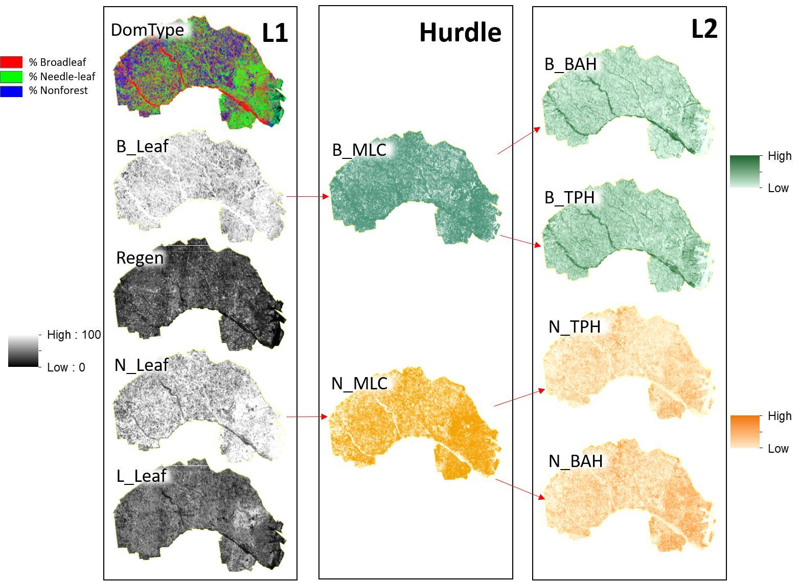
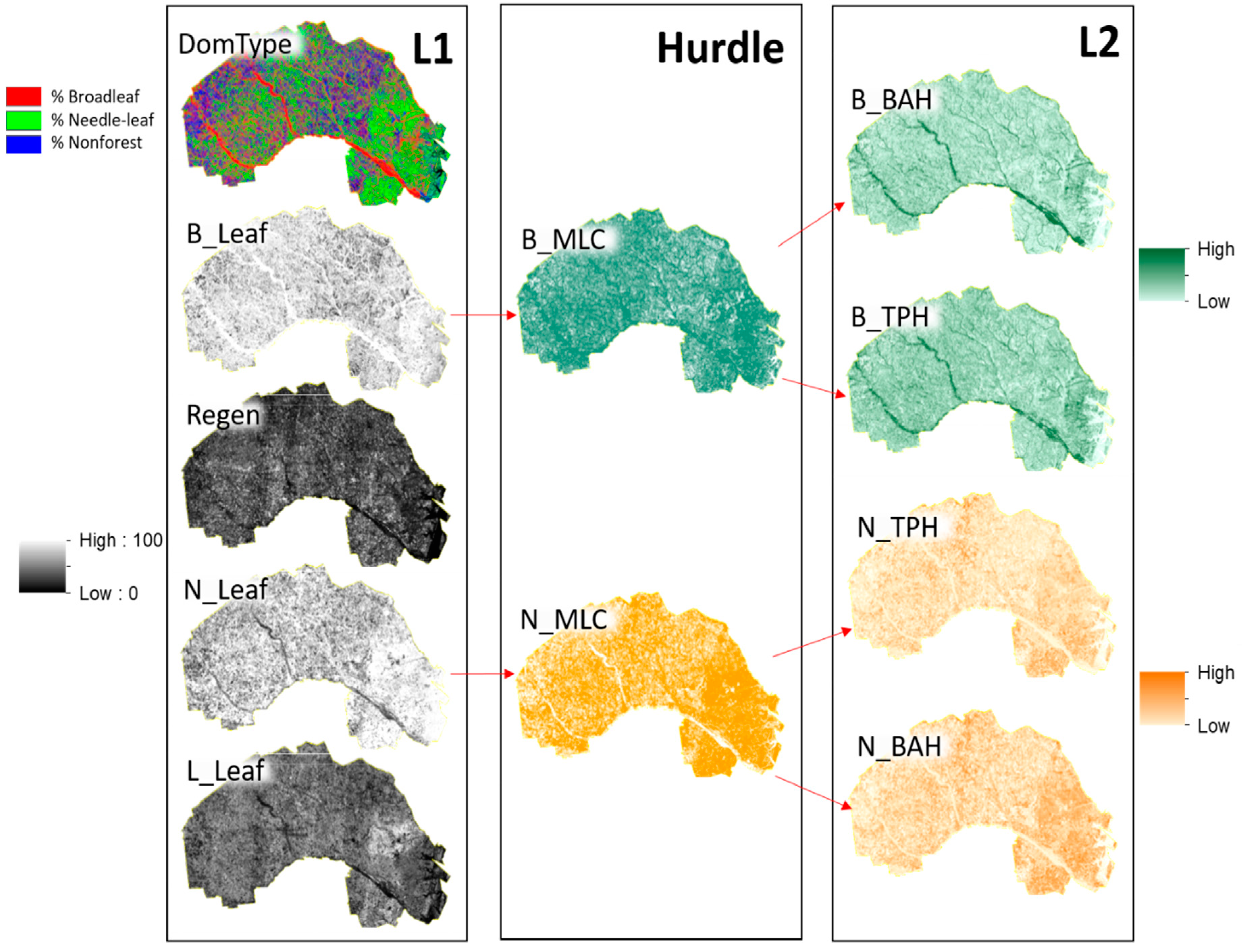
To estimate various forest characteristics, we employed a two-level hurdle modeling approach. Level 1 (L1) creates probabilistic classifications (Table 1) that quantify class probabilities for: (1) DomType, the probability of being one of three cover types (broadleaf forest, needle-leaf forest and non-forest); (2) Regen, whether trees less than 12.7 cm DBH predominantly make up the information captured within the FIA plot; (3) N_Leaf, the presence of needle-leaf trees, including longleaf pine; (4) B_Leaf, the presence of broadleaf trees; and (5) L_Leaf, the presence of longleaf pine. Level 2 (L2) then generates a suite of models that estimate transformed BAH and TPH for broad and needle-leaf tree species groups at the spatial resolution of the FIA plot, given the presence of broad (B_Leaf) or needle-leaf (N_Leaf) trees. In L2 models, the presence of broad or needle-leaf trees acts as a “hurdle” to account for zero inflation associated with plots that do not have trees present (Figure 4). For L2 estimation, B_Leaf and N_Leaf probabilistic classification model estimates (L1) are converted to presence or absence and used to constrain BAH and TPH estimates to the instances when needle or broadleaf species are present.
Transformations of predictor and response variables were used to account for non-normal distributions and linearization of the relationships between response and predictor variables. Given the skewed distributions of broad and needle-leaf continuous response variables (Figure 4), a square root and natural log transformation was applied to BAH and TPH, respectively. Transformations of predictor variable values were determined based on visual analysis of the relationship between response and predictor variables. L1 probabilistic classifications were built using multinomial (DomType) and logistic models (present\absent) while L2 and models were built using ordinary least squares multiple regression.
All analyses were performed using ESRI’s GIS [32], the RMRS Raster Utility toolbar [20,22] and the R programming language [33]. To facilitate Function Modeling within a batch processing and scripting context, we developed the “Batch Processing” tool within the RMRS Raster Utility toolbar. Using batch processing, multiple transformations to NAIP and Landsat 8 imagery were stored as small text files and occurred without writing intermediate outputs to disk, which saved processing time and storage space [5,22].
One of our study objectives was to compare finer grained NAIP based predictor variables to coarser grained Landsat 8 based predictor variables in estimating various forest characteristics. To carry out this comparison, we developed three candidate models for each response variable that were composed of NAIP only, Landsat 8 only and combined NAIP/Landsat 8 based predictor variables (27 total models). Models were then compared using Akaike information criterion (AIC) [34,35]. Due to the number of predictor variables (75), the potentially complex relationships between response and predictor variables and the degree of collinearity among predictor variables, we developed two variable selection procedures within R to help guide predictor variable selection.
The first procedure uses general additive modeling (GAM) [36] to identify predictor variables that improve model fit for binary and continuous responses (Script S1). This procedure works in a sequential fashion to add and assess potential predictor variables until all predictor variables have been exhaustively evaluated and the best fitting GAM model and predictor variables are determined, selected and returned. Unlike common stepwise procedures for variable selection, which assume a predefined relationship between response and predictor variables, this GAM routine discovers the relationship between response and predictor variables for a user defined distribution family using thin plate splines and evaluates the strength of those fitted relationships. At each iteration of our GAM variable selection procedure a potential predictor variable is added to a model (model 1) to create a candidate model (model 2). The added predictor variable within model 2 is then evaluated to determine if that variable is statistically significant at a defined alpha significance level. If the variable is not significant at the defined alpha threshold, the added predictor variable for model 2 is added to a list of removed variables and the selection procedure selects model 1 and moves to the next potential predictor variable. Otherwise, percent deviance explained for model 2 is compared against the percent deviance explained for model 1.
If the difference in percent deviance explained does not meet a defined percent increase threshold, the added predictor variable for model 2 is added to the list of removed variables and the selection procedure selects model 1 and moves to the next potential predictor variable. Otherwise, a second evaluation is performed that iteratively checks variables that have been previously removed from the selection processes to determine if any of the previously removed predictor variables are now statistically significant and the increase in percent deviance explained is greater than the set threshold given the form of model 2. If none of the previous variables are significant and the increase in percent deviance explained is less than the set thresholds, the selection procedure selects model 2 and moves to the next potential predictor variable. Otherwise, previously removed variables that meet significance and increases in percent deviance thresholds are removed from the removed variables list, added to model 2 and the selection procedure selects model 2 and moves to the next potential predictor variable.
We used this GAM selection procedure with a Binomial family and logit link distribution, alpha and increases in percent deviance thresholds of 0.1 and 0, respectively, to select potential predictor variables for L1 Regen, L_Leaf, B_Leaf and N_Leaf models. For L2, and models, this selection procedure was performed using a Gaussian family and identity link and the same alpha and percent deviance thresholds. Because GAM models can potentially over fit data, we used the results from our GAM variable selection procedure in a conservative manner to reduce the number of potential predictor variables and help identify nonlinear patterns between response and predictor variables. To select final candidate NAIP, Landsat 8 and combined NAIP/Landsat 8 based models for comparisons, we visually evaluated the subset of selected variables from the GAM procedure for variable transformations and chose predictor variables using AIC, deviance (for present\absent), residual standard errors (RSE; for continuous variables) and predictor variable p-values.
The second variable selection procedure uses the nnet package [37] to identify predictor variables that produce improved multinomial models based solely on AIC. This procedure iteratively adds predictor variables to candidate multinomial models and compares AIC statistics to previous models to determine whether an added variable not only improves a model but if the added cost of model complexity warrants the use of that variable in the model (Script S2). For DomType models we used this selection procedure and an improvement of 2 units of change in AIC statistic to select predictor variables for NAIP, Landsat 8 and combined NAIP/Landsat 8 based models.
After selecting candidate NAIP only, Landsat 8 only and combined NAIP/Landsat 8 models for each response variable, we compared model AIC statistics. In our comparisons, models with the lowest AIC values represent our best fitting models given model complexity [34]. Additionally, models with a difference in AIC value (ΔAIC) less than or equal to 2 were considered to be equivalent while ΔAIC values less than 10 suggested that models were quit similar [35]. Final model selection was based on ΔAIC values, the number of different predictor variables sources, spatial resolution and processing time associated with creating raster surfaces. To take advantage of the processing benefits of Function Modeling [22], the predictor variables selected for our final models within R were used to create equivalent models within the RMRS Raster Utility environment.
In L1, class probabilities and a most likely class (MLC) rule were used to create hard classifications [38]. To calculate hard classification accuracies and estimate classification error, we developed a bootstrapping procedure within R (Script S3). This procedure performed 5000 random selections of our data with replacement, recalibrated each of the classification models using those data, produced hard classifications and finally performed an accuracy assessment for each hard classification. Accuracy assessment cell counts were stored for each iteration and used to estimate mean cell counts and lower and upper 95% confidence limits. For final L2 models, and models were combined with L1 B_Leaf and N_Leaf hard classifications and back transformed to produce BAH and TPH estimates. Using a similar bootstrapping procedure (Script S4) as described for hard classifications, we then estimated a 95% confidence interval for the root mean squared error (RMSE) of our BAH and TPH models.
2.5. Predictions
Using the “Soft Max Nnet” tool within the RMRS Raster Utility toolbar we built five probabilistic classification models for various predictor variable combinations. The “Soft Max Nnet” tool takes user supplied tabular data with specified response and predictor variables to make a machine learning, artificial neural network classification. These neural networks are composed of linear outputs, no hidden networks and a final softmax normalization layer and produce probabilistic predictions equivalent to logistic or multinomial logistic regression [37].
These models were then used along with corresponding spectral and texture raster surfaces as inputs to the “Build Raster From Model” tool to create new raster surfaces for the full extent of the Fort Stewart SGA that provide cell estimates of class probabilities for each categorical response variable identified in Table 1. Using the “Local Stats Analysis” tool within the RMRS Raster Utility Toolbar, L1 raster surface classification probabilities and the “MAXBAND” specification, which selects the band within a multilayer raster dataset that has the largest value, we produced MLC functional raster surfaces that defined the hurdle component for the L2 models as described in Section 2.4.
Where needle or broadleaf trees were present as defined by the MLC function raster surfaces, raster surfaces depicting and were created using the “Build Raster From Model” tool, L2 RMRS Raster Utility based models derived from the “Linear Regression” tool (Table A1) and the corresponding predictor raster surfaces. and raster surface cell values were then squared and exponentiated, respectively, to produce function raster surfaces of BAH and TPH using the “Arithmetic Analysis” tool (Table A1). Cells classified as not having broad or needle-leaf trees present were given BAH and TPH values of zero. Finally, to limit cell prediction for L1 and L2 raster surfaces to the range of values used to calibrate models (i.e., no model extrapolation), we developed the “Extract Domain” tool (Table A1). This tool reads RMRS Raster Utility based models, extracts the minimum and maximums of each predictor variable based on the sample used to calibrate the model and uses those minimums and maximums to select cell values within the predictor raster surface that fall within those ranges. Cell values that have predictor variable values falling outside those ranges are populated with NULL values which can be used to identify areas where estimation would have required extrapolation outside of the values used to calibrate the models.
To take advantage of multiple central processing units (CPUs) and cores, additional tools were created and added to the RMRS Raster Utility toolbar that allow for tiling of a raster surface and saving small subsets of an otherwise large output in a parallel fashion (Table A1). Once saved, tiled outputs were mosaicked into a mosaic raster dataset and used as one large continuous dataset [21]. To aid in handling, distribution and using function raster surfaces, all L1 and L2 outputs were converted into a series of Tagged Image File Format files [39].
3. Results
3.1. Preprocessing
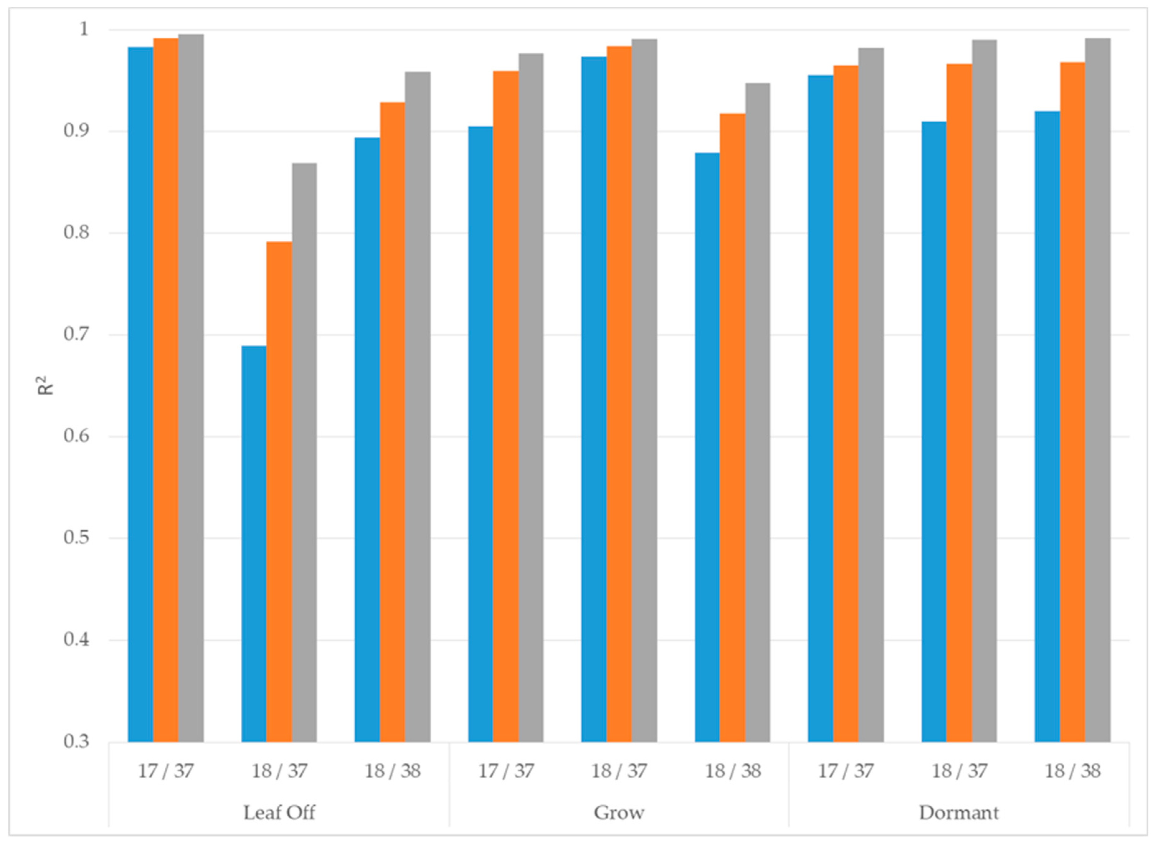
The ANR procedure brought each Landsat mosaic to a common radiometric scale with only a few bands in scene 18/37 of the leaf off phenology indicating a weak fit (Figure A2). Weak fits in the normalized images, shown as relatively low R2 values for scene 18/37 in Figure A2, were caused in large part by substantial change in land cover between Landsat acquisition dates. Once normalized, mean, standard deviation and GLCM contrast texture values for NAIP and each Landsat mosaic took seconds to create using the Function Modeling framework. Moreover, extracting those texture values and relating them to the summarized plot BAH and TPH values was also extremely quick. In total, these processes took less than two minutes to perform.
3.2. Modeling
Our findings indicate that strong relationships exist between readily available imagery and field data and that those relationships can be used to spatially characterize various aspects of a forest. Using the GAM and multinomial variable selection procedures developed in R, we were able to select three L1 and L2 candidate models based on only NAIP, only Landsat 8 and combined NAIP/Landsat 8 predictor variables (Table A3). For every response predictor variable, models that only used Landsat 8 predictor variables significantly outperformed models that only used NAIP predictor variables (Table A3). Using a ΔAIC selection threshold of 6, selected L1 models were composed of only Landsat 8 texture metrics (Table A3 and Table A4). For some of our L2 models combined NAIP/Landsat 8 predictor variables produced the best fitting models. Though a few NAIP texture bands were generally selected as statistically significant (at the α = 0.1 significance level) and improved L2 model fit when added to Landsat 8 based predictors, the amount of variation explained by NAIP predictors was relatively minor (maximum increases in R2 ~ 0.03) and did not warrant inclusion into final models given the striping phenomenon and added processing time associated with including NAIP predictors. Therefore, final L2 models only use Landsat based predictor variables to estimate BAH and TPH (Table A3).
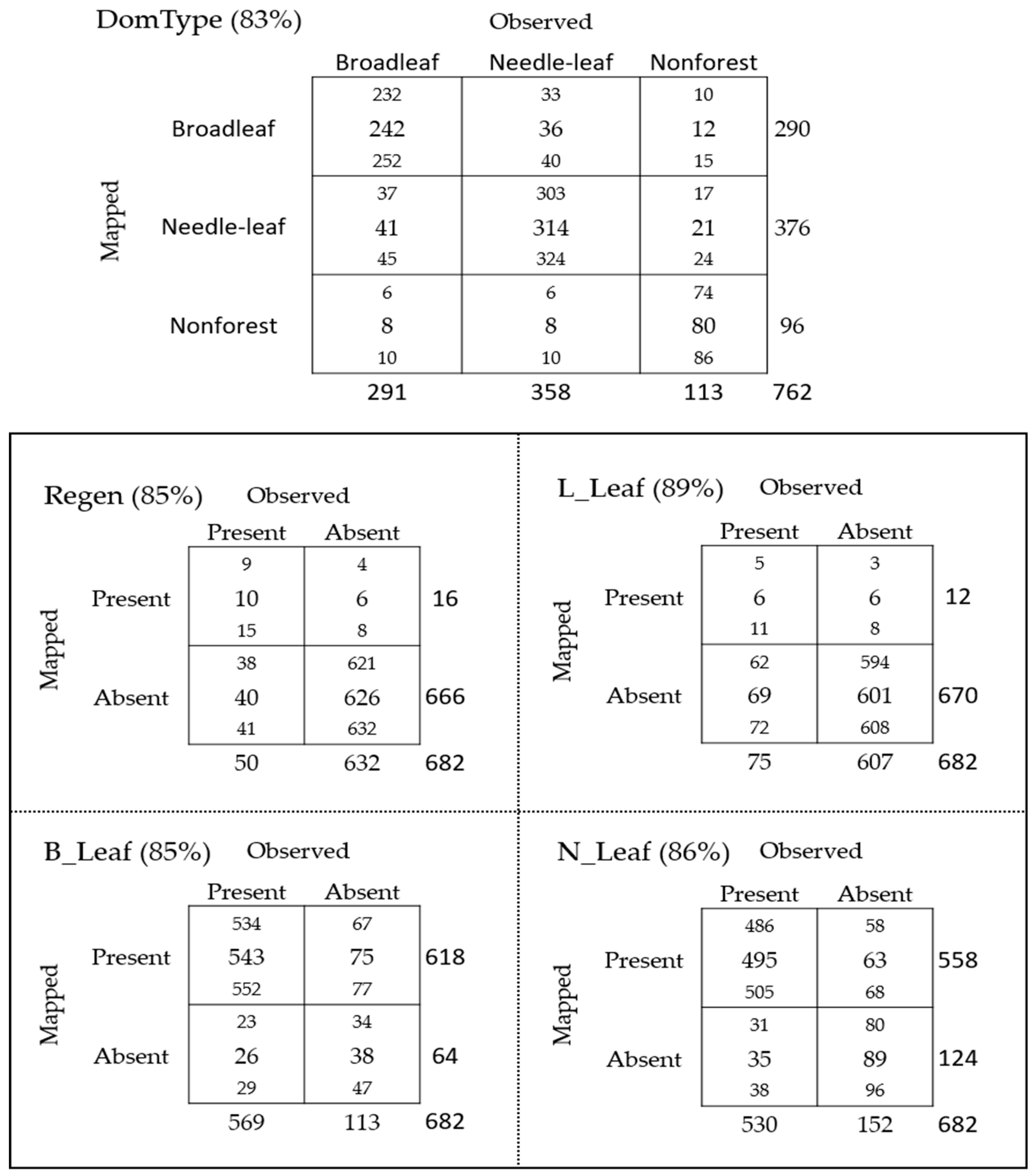
L1 models used various predictors depending on the model (Table A4) and explained a statistically significant portion of the information within the data, with model deviance ranging from 258 for the Regen model to 794 for the DomType model (Table 2). Applying an MLC rule to L1 class probabilities we created five hard classification accuracy assessments which had high overall map accuracies (>80%; Figure 6). Estimated 95% confidence intervals for each cell within each accuracy assessment are reported in Figure 6 and provide a lower and upper frequency estimate that can be used to determine with 95% confidence the total area associated with each hard classification category in the Fort Stewart SGA.
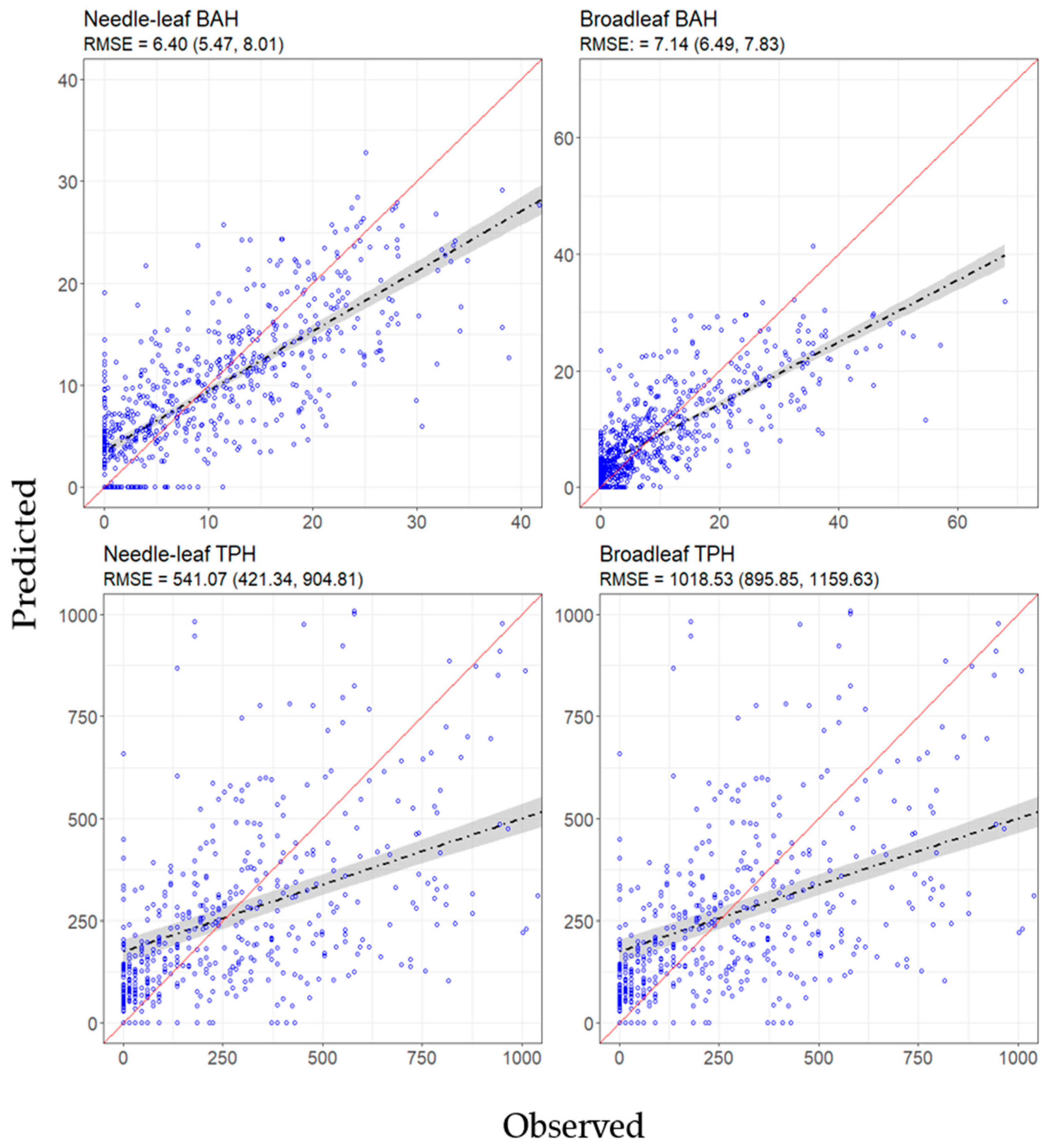
L2 and models were also statistically significant and had R2 values varying from 0.266 to 0.574 (Table 2). In all, two and two models were created conditioned on the presence of needle and broadleaf trees (Table 2). To evaluate L2 hurdle models of BAH and TPH, we compared the combination of B_Leaf and L_Leaf hard classifications and back transformed and estimates with plot based measures of BAH and TPH estimates, respectively. RMSE for needle and broadleaf BAH hurdle models were 6.40 and 7.14, respectively. For needle and broadleaf TPH hurdle models, RMSE statistics were 541.07 and 1018.53, respectively. Observed versus fitted values and bootstrapped estimates of 95% RMSE confidence intervals are reported in Figure 7.
3.3. Prediction
Using the “Build Raster From Model” tool, Landsat 8 predictor surfaces and the “Save Raster” tool, we built one multilayer, 3-band raster dataset (DomType; with bands for broadleaf, needle-leaf and non-forest) and four single band raster datasets (Regen, B_Leaf, N_leaf and L_Leaf) that estimate the probability of each L1 class occurring for every raster cell across the SGA at the spatial resolution of 30 m (Figure 8, Figure A3 and Figure A4, Table 2). Applying an MLC rule to N_Leaf and B_Leaf class probabilities, we created two different hard classification function raster surfaces (Figure 8 and Figure A3). These surfaces were used as a spatial masks (hurdle) for the creation of L2 raster surfaces (Figure 8 and Figure A4).
Unexpectedly, FIA plot locations did not capture the entire range of values of the imagery-derived predictor variables across the study area. In these instances, L1 and L2 cell predictions represent extrapolations of the modeled results and are unreliable. In the final L1 and L2 raster surfaces, extrapolated cells were populated with NULL values using the “Extract Model Domain” tool (Table A3, Figure A3 and Figure A4). While modeled relationships were a significant improvement over classical spatial aggregation techniques such as FIA plot summaries (i.e., Figure 4 standard deviation verses Figure 7 RMSE) and are an improvement over previous longleaf mapping projects that include striping [10,12], there was more variability in the relationships than we anticipated. Sources of variation are discussed in Section 4.
4. Discussion
One of the primary outputs of this project was a series of fine grain raster surfaces depicting various forest characteristics stored in a common digital format [39]. While the grain size of L1 and L2 raster surfaces is 30 m (900 m2), L1 and L2 surfaces have a nominal spatial resolution equal to the extent of an FIA plot (78 m by 70 m). Additionally, to meet project objectives, facilitate the replication of these study methods and prioritize restoration efforts, multiple tutorials and many new raster and vector processing tools were developed and made available online to stakeholders, practitioners and the public [20,40].
These datasets can be integrated with existing tabular, vector and raster data using spatial analyses found within most widely used GIS. In addition, many of the tools within the RMRS Raster Utility toolbar [20] can perform spatial analyses and tabular summaries of spatial data with enhanced functionality, such as manipulating large multi-band raster datasets. Several tutorials have been developed and are available to provide examples and guide the use of these tools, techniques and data for restoration efforts [40]. Moreover, tutorials demonstrate how to use modeling error to accurately account for variation within the modeled outputs. Datasets, tutorials and the RMRS Raster Utility can all be accessed online through the RMRS Raster Utility Website [20] and associated data hosting services [39].
We were able to significantly improve estimates of the amount, location and condition of longleaf pine and other forest ecosystems across the Fort Stewart SGA using Landsat 8 imagery and FIA field data. Similar to other studies that relate field data with remotely sensed information to estimate aspects of the forested condition, BAH tended to be more strongly correlated with spectral metrics than TPH [12,41,42,43]. Additionally, our study also supports the idea that multi-temporal imagery and finer resolution imagery such as NAIP provides additional information over using only single season imagery when predicting forest characteristics [41,44]. However, due to the NAIP image mosaicking process, NAIP based predictor variables provided less information than we anticipated in many of our models and also contained added spatial variability, making raster surfaces derived from those predictor variables less desirable from an applied perspective. For these reasons, the final model used only Landsat 8 based predictor variables.
Compared to our previous studies [10,12], which used only NAIP based texture to estimate similar forest characteristics as in this study, the models and outputs of this study are an improvement. For similar classifications and models of BAH and TPH, overall map accuracy was improved and RMSEs normalized by mean values of BAH and TPH were smaller. Moreover, in this study neither striping nor scene boundaries were present in the resulting raster datasets. Though there was error associated with our estimates of presence and absence, basal area and stand density, the associated raster outputs can be used in multiple ways to quantify and locate high quality longleaf and potential longleaf habitat sites efficiently and effectively (e.g., [40]). While our current models and outputs are a significant improvement over classical aggregation techniques (especially simple FIA plot summaries) and previous mapping efforts [10,12], there are potentially many ways to further improve our estimates and reduce the amount of error in the outputs.
To better understand how we can accomplish those improvements, it helps to look at two primary sources of variability within the data: (1) differences in Landsat acquisition dates and corresponding land use change and (2) the FIA field sampling protocol as it relates to remotely sensed imagery. First, differences in spectral reflectance for Landsat scenes were minimized in large part by using ANR. However, some bands in path/row 18/37 acquired during a leaf off phenology had coefficients of determination lower than 0.8, suggesting that those bands were not completely normalized to a common radiometric scale. This was most likely due to the amount of land use change that occurred between reference and subject images. Fortunately, that path/row when mosaicked in the order described accounted for only a small portion of the area examined in this study.
The second source of variation relates to the spatial accuracy of Landsat 8 imagery, the grain size of the imagery, FIA plot locations and the FIA field sampling protocol. Landsat 8 imagery is orthorectified with an image to image RMSE that is generally less than one pixel [45]. While this is exceptional, each Landsat pixel has a grain size of 900 m2, potentially adding significant spatial error to the alignment with forest inventory plots. Additionally, a FIA plot covers approximately half a ha (78 m by 70 m) and is composed of four subplots with radii of 7.32 m for trees greater than or equal to 12.7 cm in DBH and four subplots with radii of 2.07 m for trees less than 12.7 cm in DBH. Within the extent of an FIA plot footprint, this means that approximately 12% of the area of the plot is measured for trees greater than or equal to 12.7 cm in DBH and less than 1% of the area is measured for trees less than 12.7 cm in DBH. This suggests that for the extent of a FIA plot there can be substantial variation in summarized estimates and that estimated mean values can vary significantly from true mean values, especially for trees less than 12.7 cm in DBH occurring on heterogeneous plots. To draw stronger relationships between plot measurements and Landsat 8 metrics, plots should be sampled using a design that covers more of the extent of the plot [46] than what is currently specified within the FIA plot protocol [24]. Furthermore, field plot layouts, such as described in Reference [46], should also help to improve the accuracy and precision of models that link field plot data to imagery.
In our study NAIP based predictors were not used to produce final predictive models and L1 and L2 raster surfaces. Despite its high spatial resolution, NAIP was not as good of a predictor source as Landsat 8 imagery. This is most likely due to the varying times of image acquisition and the cosmetic color balancing process used to blur the image seamlines. Combined with Landsat 8 imagery, NAIP texture (standard deviation and horizontal contrast) showed some improvement in model fit. However, it was relatively minor and did not warrant the additional complexity associated with generating and including NAIP predictors in the final models. Interestingly, NAIP and Landsat 8 mean texture values at the spatial resolution of a FIA plot were strongly correlated with one another. This suggests that if raw, unprocessed NAIP imagery can be acquired, a modified ANR procedure that uses coarser grained Landsat 8 imagery could be used to bring NAIP images to a common radiometric scale and those normalized images could be used to produce predictor variables free from the color balancing issues associated with the current NAIP mosaicking process. The authors are currently conducting such an analysis for the Apalachicola region of Florida using NAIP imagery that has not been rectified, compressed, mosaicked or color balanced and expect better results using raw NAIP data.
Finally, because L1 and L2 outputs have modeling error, care should be taken when using the outputs. For small areas of the landscape (i.e., less than 40 ha), aggregated mean cell values can vary substantially. However, for larger areas (i.e., greater than 400 ha), aggregated cell values should closely approximate the true mean condition of that area. Use of these surfaces for longleaf restoration should consider this in developing restoration strategies.
5. Conclusions
Our Landsat 8 based models linked FIA plot data to image based texture and explained a substantial amount of variation in the field data. Additionally, they are an improvement over aggregating FIA plot information to produce area estimates of longleaf pine cover. Furthermore, they offer some improvement over previous mapping attempts that used only NAIP imagery [10,12]. Most important, the models and outputs created from this study can be used to identify where longleaf pine trees are present within the Fort Stewart SGA and quantify the condition and characteristics of various forest types for much smaller spatial extents than was previously possible. These outputs can be combined, transformed and summarized to address a wide range of restoration questions and are available online for free [39].
Supplementary Materials
The following are available online at https://www.mdpi.com/2072-4292/11/15/1803/s1, Script S1: getGamSigFldNames.R, Script S2: getPlrSigFldNames.R, Script S3: bootStrappedAA.R, Script S4: hurdleBootRmse.R.
Author Contributions
J.H. proposed, built and applied the tools developed in the study. He also designed and implemented significant parts of the analysis described. He was the lead author of the manuscript. N.A. provided project oversight and contributed to writing portions of the manuscript. D.L.R.A. provided technical assistance and guidance and review of the manuscript. J.S.P. provided technical assistance with analyzing data, developing the raster surfaces and writing portions of the manuscript.
Funding
This research received no external funding but the Authors gratefully acknowledge financial support from the U.S. Forest Service, specifically State and Private Forestry, the Southern Region and the Rocky Mountain Research Station. Additional support for the development of the RMRS Raster Utility, which was used extensively in this research, was provided by the Agriculture and Food Research Initiative Competitive Grant 2013-68005-21298 from the USDA National Institute of Food and Agriculture through the Bioenergy Alliance Network of the Rockies (BANR).
Acknowledgments
The Authors would like to thank Kay Reed, Jamie Barbour, Jason Drake and Paul Medley for their encouragement and for their interest and dedication to longleaf pine conservation and management throughout the southeastern United States. Additionally, we would like to thank the three independent reviewers and Melissa Reynolds-Hogland. Their comments and suggestions helped to significantly improve this article.
Conflicts of Interest
The Authors declare no conflict of interest.
Appendix A. Tables and Figures

Table A1.
List of newly developed tools integrated into the RMRS Raster Utility toolbar and used to faciliate raster and vector based processing.
Table A1.
List of newly developed tools integrated into the RMRS Raster Utility toolbar and used to faciliate raster and vector based processing.
| Name | Icon | Description |
|---|---|---|
| Download Data |  | The “Download Data” tool is a standalone executable that automates FTP based NAIP image downloads. It has an easy to use graphical user interface that allows users to select existing feature classes, specify FTP sites and define where images will be stored on disk. |
| Map Services Download |  | The “Map Services Download” tool allows users to extract information from a map service for a given area of interest and create a local copy of that information within a ESRI file geodatabase. |
| Summarize FIA Data |  | The “Summarize FIA Data” tool summarized FIA tree data formatted within a Microsoft Access database to plot and subplot area estimates for user specified species, condition and status grouping. The tool allows users to specify a formatted FIA database and will relate summarized FIA tree data to a point feature class. |
| Aggregate no-change regression (ANR) |  | The “Aggregate no-change regression (ANR)” tool performs a relative image normalization routine given the overlapping regions between two images [29]. |
| Focal Analysis |  | The “Focal Analysis” tool performs various moving window focal analyses for user specified windows and raster surfaces. Outputs from the tool are stored as function raster surfaces. |
| GLCM Analysis |  | The “GLCM Analysis” tool performs various moving window GLCM analyses for user specified windows and raster surfaces. Outputs from the tool are stored as function raster surfaces. |
| Sample Values |  | This tool uses the spatial coordinates of a given point feature class to extract the coincident values from raster and vector datasets and append those values to the attribute table of the point feature class. |
| Batch Processing |  | The “Batch processing” tool allows users to create and store small text files (batch files) that list a series of RMRS Raster Utility commands used to read spatial data, perform a series of tasks and display the results of those tasks as function raster datasets. |
| Soft Max Nnet |  | The “Soft Max Nnet” tool takes user supplied tabular data with specified response and predictor variables and makes a machine learning, artificial neural network classification model. |
| Build Raster From Model |  | The “Build Raster From Model” tool takes a user selected predictive model and corresponding raster based predictor surfaces to create new function raster surfaces [22] depicting class probabilities. |
| Local Stats Analysis |  | The “Local Stats Analysis” tool performs band based statistics for each cell given a user specified multilayer raster and statistic. Outputs from the tool are stored as function raster surfaces. |
| Linear Regression |  | The “Linear Regression” tool takes user supplied tabular data with specified response and predictor variables and makes an ordinary least squares regression model. |
| Arithmetic Analysis |  | The “Arithmetic Analysis” tool performs arithmetic at the raster cell level defined by the user for specified raster datasets. |
| Extract Domain | Batch Proccessing command | The “Extract Domain” tool populates raster cell values with a NULL value for instances that a predictive model is extrapolating. Users specify a RMRS Raster Utility based model and the raster predictor variable surfaces used to create the model. |
| Save Parellel |  | The “Save Parallel” tool reads a raster dataset including batch files and saves those datasets as smaller subsets defined by the user in a parallel fashion. |
Table A2.
Groups of trees species used in this study based on FIA tree species codes [24].
Table A2.
Groups of trees species used in this study based on FIA tree species codes [24].
| Group Name | FIA Species Codes |
|---|---|
| Needle-leaf | 115, 128, 131, 107, 110, 111, 121(Longleaf pine) |
| Broadleaf | 819, 835, 838, 842, 806, 824, 840, 841, 68, 221, 222, 802, 812, 813, 820, 825, 827, 831, 837, 822, 833, 834, 461, 462, 491, 521, 531, 544, 555, 591, 611, 621, 652, 653, 682, 691, 692, 693, 694, 711, 721, 762, 858, 922, 931, 972, 975, 993, 999, 316, 373, 391, 311, 317, 323, 345, 356, 367, 381, 421, 471, 500, 502, 541, 548, 551, 552, 581, 660, 662, 681, 701, 722, 731, 760, 764, 766, 901, 912, 953, 971, 994, 402, 403, 404, 409, 401, 410 |
Table A3.
Model, data source for predictors, number of predictors, AIC, delta AIC and deviance and coefficient of determination (R2) of candidate NAIP only, Landsat 8 only and combined NAIP/ Landsat 8 based models.
Table A3.
Model, data source for predictors, number of predictors, AIC, delta AIC and deviance and coefficient of determination (R2) of candidate NAIP only, Landsat 8 only and combined NAIP/ Landsat 8 based models.
| Model | Source | Predictors | AIC | ΔAIC | Deviance\R2 |
|---|---|---|---|---|---|
| DomType | Landsat 8 | 20 | 878.64 | - | 794.64 |
| NAIP | 10 | 1039.03 | 160.39 | 995.03 | |
| NAIP/Landsat 8 | 60 | 967.33 | 88.69 | 723.33 | |
| Regen | Landsat 8 | 7 | 273.94 | 5.29 | 257.94 |
| NAIP | 5 | 313.22 | 44.57 | 301.22 | |
| NAIP/Landsat 8 | 8 | 268.65 | - | 250.65 | |
| N_Leaf | Landsat 8 | 6 | 460.15 | - | 446.15 |
| NAIP | 5 | 651.37 | 191.22 | 639.37 | |
| NAIP/Landsat 8 | 8 | 464.20 | 4.05 | 444.20 | |
| B_Leaf | Landsat 8 | 4 | 418.85 | 4.12 | 408.85 |
| NAIP | 4 | 558.25 | 143.52 | 548.25 | |
| NAIP/Landsat 8 | 6 | 414.73 | - | 400.73 | |
| L_Leaf | Landsat 8 | 5 | 408.60 | - | 396.60 |
| NAIP | 3 | 464.92 | 56.32 | 456.92 | |
| NAIP/Landsat 8 | 5 | 408.60 | 0.00 | 396.60 | |
| N_BAH | Landsat 8 | 9 | 1460.17 | 40.15 | 0.52 |
| NAIP | 5 | 1723.14 | 303.12 | 0.20 | |
| NAIP/Landsat 8 | 10 | 1420.02 | - | 0.55 | |
| B_BAH | Landsat 8 | 11 | 1717.67 | 18.09 | 0.57 |
| NAIP | 5 | 2118.65 | 419.07 | 0.12 | |
| NAIP/Landsat 8 | 10 | 1699.58 | - | 0.58 | |
| N_TPH | Landsat 8 | 10 | 1496.56 | 35.80 | 0.46 |
| NAIP | 4 | 1673.15 | 212.39 | 0.23 | |
| NAIP/Landsat 8 | 11 | 1460.76 | - | 0.49 | |
| B_TPH | Landsat 8 | 6 | 1706.39 | - | 0.27 |
| NAIP | 4 | 1835.78 | 129.39 | 0.07 | |
| NAIP/Landsat 8 | 6 | 1706.39 | 0.00 | 0.27 |
Table A4.
Response and predictor variables selected in final L1 and L2 forest characteristics models.
Table A4.
Response and predictor variables selected in final L1 and L2 forest characteristics models.
| Model | Response | Image Phenology | Texture | Bands & Transformations |
|---|---|---|---|---|
| DomType | Broadleaf, Needle-leaf, Non-forest | Dormant | Mean | 2, 3, 6 |
| Contrast | 1, 3, 4, 7 | |||
| Grow | Mean | 2, 3, 4, 5, 7 | ||
| SD | 5 | |||
| Contrast | 5 | |||
| Off | Mean | 6,7 | ||
| Contrast | 1, 2, 5, 7 | |||
| N_Leaf | Present/Absent | Dormant | Mean | 5, 6 |
| Grow | SD | 5 | ||
| Off | Mean | 5, 6 | ||
| SD | 6 | |||
| B_Leaf | Present/Absent | Grow | Mean | 5, ln(4) |
| SD | 1 | |||
| Off | Mean | 5 | ||
| L_Leaf | Present/Absent | Dormant | Mean | 2, 3, 5 |
| Grow | Mean | 5 | ||
| Off | Mean | 5 | ||
| Regen | Present/Absent | Dormant | Mean | 2, 3, 6 |
| Grow | Mean | 5 | ||
| Off | Mean | 1, 3, 5 | ||
| N_BAH | Dormant | Mean | ln(4), ln(6) | |
| Grow | Mean | ln(3), ln(6) | ||
| Contrast | 6, ln(2) | |||
| Off | Mean | 5, ln(4) | ||
| SD | ln(3) | |||
| N_TPH | Dormant | Mean | 3, ln(6) | |
| SD | ln(4) | |||
| Contrast | 6 | |||
| Grow | Mean | ln(3), ln(6) | ||
| Contrast | ln(4) | |||
| Off | Mean | 5, ln(4) | ||
| SD | 4 | |||
| B_BAH | Dormant | Mean | ln(3), ln(6) | |
| SD | 1 | |||
| Grow | Mean | ln(3), ln(4) | ||
| SD | 7 | |||
| Off | Mean | 1, ln(3), ln(5) | ||
| Contrast | 4, 5 | |||
| B_TPH | Dormant | Contrast | ln(1) | |
| Grow | Mean | ln(4), ln(5) | ||
| SD | 1, 5 | |||
| Off | Mean | ln(5) |
Figure A1.
Example of visible scene boundary between two Landsat 8 images for the Growing phenology after converting DN values to surface reflectance [28]. Images have been mosaicked together with no blending of pixels values like in Figure 5 and are displayed in red, green and blue (RGB), color composites for specified band combinations.

Figure A2.
Minimum (blue), average (orange) and maximum (gray) coefficient of determination (R2) values for each Landsat path/row (x-axis) and phenology (x-axis title) using the ANR relative normalization process.
Figure A2.
Minimum (blue), average (orange) and maximum (gray) coefficient of determination (R2) values for each Landsat path/row (x-axis) and phenology (x-axis title) using the ANR relative normalization process.

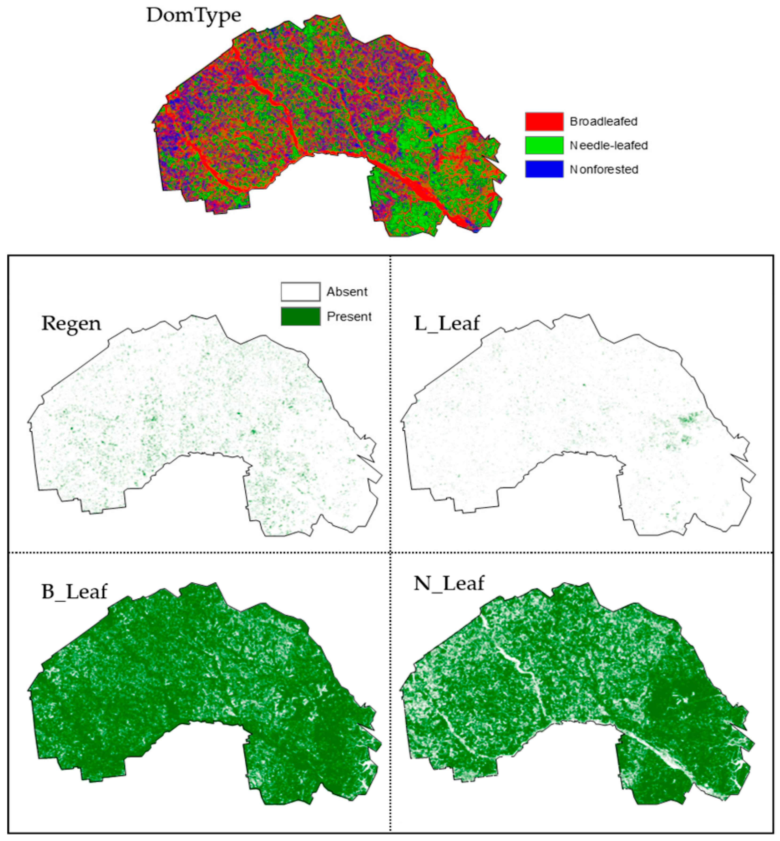
Figure A3.
L1 Dominant forest type (DomType) and presence/absence hard classification raster surfaces for areas containing longleaf pine trees (L_Leaf), areas composed of mostly regeneration (Regen), areas containing needle-leaf trees (N-Leaf) and areas contain broadleaf trees within the Fort Stewart SGA. L1 probability surfaces and a most likely class (MLC) rule were used to create each hard classification. Hard classification map accuracies can be found in Figure 6.

Figure A4.
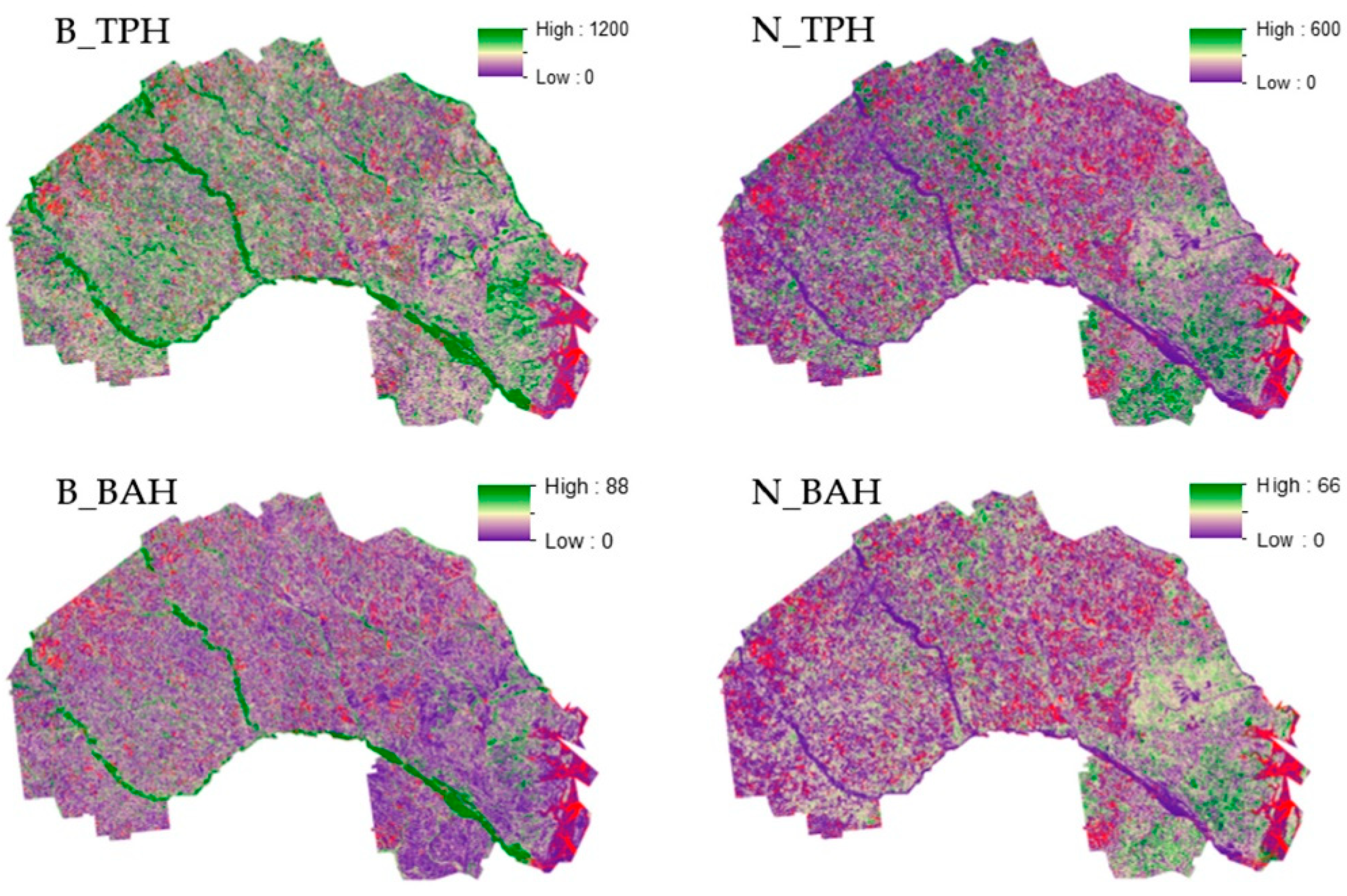
L2 Broad and needle-leaf TPH and BAH raster surfaces for the Fort Stewart SGA. Red areas within each graphic identify locations for which L2 models extrapolate estimates. Cell values for these areas are coded as NULL.
Figure A4.
L2 Broad and needle-leaf TPH and BAH raster surfaces for the Fort Stewart SGA. Red areas within each graphic identify locations for which L2 models extrapolate estimates. Cell values for these areas are coded as NULL.

References
- Noss, R.; LaRoe, E.; Scott, J. Endangered Ecosystems of the United States: A Preliminary Assessment of Loss and Degradation; Biological Report 28; National Biological Service: Washington, DC, USA, 1995. Available online: https://sciences.ucf.edu/biology/king/wp-content/uploads/sites/106/2011/08/Noss-et-al-1995.pdf (accessed on 19 July 2019).
- Oswalt, C.; Cooper, J.; Brockway, D.; Brooks, H.; Walker, J.; Connor, K.; Oswalt, S.; Conner, R. History and Current Condition of Longleaf Pine in the Southern United States; USDA Forest Service General Technical Report SRS-166; United States Forest Service: Ashville, NC, USA, 2012. Available online: http://www.srs.fs.usda.gov/pubs/42259 (accessed on 6 February 2019).
- Regional Working Group for America’s Longleaf. Range-Wide Conservation Plan for Longleaf. 2009. Available online: http://www.americaslongleaf.org/media/86/conservation_plan.pdf (accessed on 6 February 2019).
- Longleaf Partnership Council. America’s Longleaf Restoration Initiative 2013; Range-Wide Accomplishment Report, Final Report; Longleaf Alliance: Andalusia, AL, USA, 2014; Available online: http://www.longleafalliance.org/publications/2013RangewideAccomplishmentReport_2_12_FINAL.pdf (accessed on 6 February 2019).
- Hogland, J.S.; Anderson, N.M.; Chung, W.; Wells, L.A. Estimating forest characteristics using NAIP imagery and ArcObjects. In Proceedings of the 2014 ESRI Users Conference, San Diego, CA, USA, 14–18 July 2014; Environmental Systems Research Institute: Redlands, CA, USA, 2014. Available online: https://www.fs.usda.gov/treesearch/pubs/46333 (accessed on 6 February 2019).
- Wells, L.A.; Chung, W.; Anderson, N.M.; Hogland, J.S. Spatial and temporal quantification of forest residue volumes and delivered costs. Can. J. For. Res. 2016, 46, 832–843. Available online: https://www.fs.usda.gov/treesearch/pubs/50967 (accessed on 6 February 2019). [CrossRef]
- Hogland, J.S.; Anderson, N.M. Estimating FIA plot characteristics using NAIP imagery, function modeling, and the RMRS Raster Utility coding library. In Forest Inventory and Analysis (FIA) Symposium 2015, General Technical Report, PNW-GTR-931; U.S. Department of Agriculture, Forest Service, Pacific Northwest Research Station: Portland, OR, USA, 2015; pp. 340–344. Available online: https://www.fs.usda.gov/treesearch/pubs/50147 (accessed on 6 February 2019).
- Hogland, J.S.; Anderson, N.M.; Chung, W. New geospatial approaches for efficiently mapping forest biomass logistics at high resolution over large areas. ISPRS Int. J. Geo-Inf. 2018, 7, 156. Available online: https://www.mdpi.com/2220-9964/7/4/156 (accessed on 6 February 2019). [CrossRef]
- National Agriculture Imagery Program, National Agriculture Imagery Program (NAIP) Information Sheet. August 2013. Available online: http://www.fsa.usda.gov/Internet/FSA_File/naip_info_sheet_2013.pdf (accessed on 6 February 2019).
- St. Peter, J.; Hogland, J.; Anderson, N.; Drake, J.; Medley, P. Fine resolution probabilistic land cover classification of landscapes in the southeastern United States. ISPRS Int. J. Geo-Inf. 2018, 7, 107. Available online: https://www.mdpi.com/2220-9964/7/3/107 (accessed on 6 February 2019). [CrossRef]
- U.S. Forest Service Forest Inventory and Analysis Program: We Are the Nation’s Forest Census. Available online: https://www.fia.fs.fed.us/ (accessed on 6 February 2019).
- Hogland, J.; Anderson, N.; St. Peter, J.; Drake, J.; Medley, P. Mapping forest characteristics at fine resolution across large landscapes of the southeastern United States using NAIP imagery and FIA field plot data. ISPRS Int. J. Geo-Inf. 2018, 7, 140. Available online: https://www.mdpi.com/2220-9964/7/4/140/htm (accessed on 6 February 2019). [CrossRef]
- America’s Longleaf. The America’s Longleaf Restoration Initiative. Available online: http://www.americaslongleaf.org/ (accessed on 6 February 2019).
- The Longleaf Alliance. The Fort Stewart/Altamaha Longleaf Partnership. Available online: https://www.longleafalliance.org/fsalp/about-ft.-stewart-altamaha-longleaf-partnership (accessed on 6 February 2019).
- U.S. Forest Service, Forest Inventory and Analysis (FIA). Database, U.S. Department of Agriculture, Forest Service; Northern Research Station: Saint Paul, MN, USA, 2019. Available online: https://apps.fs.usda.gov/fia/datamart/datamart.html (accessed on 6 February 2019).
- U.S. Forest Service, Forest Inventory and Analysis (FIA). Spatial Data Request. Available online: https://www.fia.fs.fed.us/tools-data/spatial/requests/index.php (accessed on 6 February 2019).
- U.S. Geological Survey File Transfer Protocol. Staged NAIP Data. Available online: Ftp://rockyftp.cr.usgs.gov/vdelivery/Datasets/Staged/NAIP/ (accessed on 6 February 2019).
- U.S. Geological Survey. Earth Explorer. Available online: https://earthexplorer.usgs.gov/ (accessed on 6 February 2019).
- U.S. Geological Survey. Landsat 8. Available online: https://landsat.gsfc.nasa.gov/landsat-8/ (accessed on 19 July 2019).
- U.S. Forest Service, Rocky Mountain Research Station. RMRS Raster Utility. Available online: http://www.fs.fed.us/rm/raster-utility (accessed on 6 February 2019).
- Environmental Systems Research Institute (ESRI). What is a Mosaic Raster Dataset? ESRI ArcPress: Redlands, CA, USA; Available online: http://desktop.arcgis.com/en/arcmap/10.3/manage-data/raster-and-images/what-is-a-mosaic-dataset.htm (accessed on 6 February 2019).
- Hogland, J.; Anderson, N. Function Modeling Improves the Efficiency of Spatial Modeling using Big Data from Remote Sensing. Big Data Cogn. Comput. 2017, 1, 3. Available online: https://www.mdpi.com/2504-2289/1/1/3 (accessed on 6 February 2019). [CrossRef]
- Hogland, J.; Anderson, N. Improved analyses using function datasets and statistical modeling. In Proceedings of the 2014 ESRI Users Conference, San Diego, CA, USA, 14–18 July 2014; Environmental Systems Research Institute: Redlands, CA, USA, 2014. Available online: https://www.fs.fed.us/rm/pubs_other/rmrs_2014_hogland_j001.pdf (accessed on 7 July 2019).
- U.S. Forest Service Forest Inventory and Analysis (FIA) National Core Field Guide: Field Data Collection Procedures for Phase 2 Plots, Version 6.0, Vol. 1, Internal Report. Available online: http://www.fia.fs.fed.us/library/field-guides-methods-proc/docs/2013/Core%20FIA%20P2%20field%20guide_6-0_6_27_2013.pdf (accessed on 6 February 2019).
- Gao, F.; Masek, J.; Schwaller, M.; Hall, F. On the blending of the Landsat and MODIS surface reflectance: Predicting daily Landsat surface reflectance. IEEE Trans. Geosci. Remote Sens. 2006, 44, 2207–2218. [Google Scholar]
- Hilker, T.; Wulder, M.; Coops, N.; Sietz, N.; White, J.; Gao, F.; Masek, J.; Stenhous, G. Generation of dense time series synthetic Landsat Data through data blending with MODIS using a spatial and temporal adaptive reflectance fusion model. Remote Sens. Environ. 2009, 113, 1988–1999. [Google Scholar] [CrossRef]
- Weng, Q.; Fu, P.; Gao, F. Generating daily land surface temperature at Landsat resolution by fusing Landsat and MODIS data. Remote Sens. Environ. 2014, 145, 55–67. [Google Scholar] [CrossRef]
- U.S. Geological Survey. Landsat 8 Surface Reflectance Code (LASRC) Product Guide. General Technical Report LSDS-1368 Version 2.0; 2019. Available online: https://prd-wret.s3-us-west-2.amazonaws.com/assets/palladium/production/atoms/files/LSDS-1368_L8_Surface_Reflectance_Code_LASRC_Product_Guide-v2.0.pdf (accessed on 19 July 2019).
- Hogland, J. Creating Spatial Probability Distributions for Longleaf Pine Ecosystems across East Mississippi, Alabama, The Panhandle of Florida and West Georgia. Master’s Thesis, Auburn University, Auburn, AL, USA, 2005. Available online: http://etd.auburn.edu/handle/10415/603 (accessed on 6 February 2019).
- Elvidge, C.D.; Yuan, D.; Weerackoon, R.D.; Lunneta, R.S. Relative radiometric normalization of Landsat Multispectral Scanner (MSS) data using an automatic scattergram-controlled regression. Photogramm. Eng. Remote Sens. 1995, 61, 1255–1260. [Google Scholar]
- Haralick, R.; Shanmugam, K.; Dinstein, I. Texture features for image classification. IEEE Trans. Syst. Manand Cybern. 1973, 3, 610–621. [Google Scholar] [CrossRef]
- Environmental Systems Research Institute (ESRI). About ArcGIS: The Mapping and Analytics Platform. Available online: https://www.esri.com/en-us/arcgis/about-arcgis/overview (accessed on 6 February 2019).
- The R Project for Statistical Computing; R Foundation for Statistical Computing: Vienna, Austria; Available online: http://www.R-project.org/ (accessed on 6 February 2019).
- Akaike, H. Information theory and an extension of the maximum likelihood principle. In Proceedings of the 2nd International Symposium on Information Theory, Tsahkadsor, Armenia, 2–8 September 1971; Petrov, B.N., Csaki, F., Eds.; Akadémiai Kiadó: Budapest, Hungary, 1973; pp. 267–281. [Google Scholar]
- Akaike, H. A new look at the statistical model identification. IEEE Trans. Autom. Control 1974, 19, 716–723. [Google Scholar] [CrossRef]
- Wood, S.N. Fast stable restricted maximum likelihood and marginal likelihood estimation of semiparametric generalized linear models. J. R. Stat. Soc. 2011, 73, 3–36. [Google Scholar] [CrossRef]
- Venables, W.N.; Ripley, B.D. Modern Applied Statistics with S, 4th ed.; Springer: New York, NY, USA, 2002; ISBN 0-387-95457-0. [Google Scholar]
- Hogland, J.; Billor, N.; Anderson, N. Comparison of standard maximum likelihood classification and polytomous logistic regression used in remote sensing. Eur. J. Remote Sens. 2013, 46, 623–640. [Google Scholar] [CrossRef] [Green Version]
- Hogland, J.; St. Peter, J.; Anderson, N. Raster Surfaces Created from the Mapping of Longleaf Extent and Condition Using Landsat and FIA Data, U.S. Forest Service, Research Data Archive. Available online: https://www.fs.usda.gov/rds/archive/Product/RDS-2018-0039/ (accessed on 6 February 2019).
- U.S. Forest Service. Rocky Mountain Research Station. RMRS Raster Utility Tutorials. Available online: https://www.fs.fed.us/rm/raster-utility/tutorials/ (accessed on 6 February 2019).
- Shang, C.; Treitz, P.; Caspersen, J.; Jones, T. Estimation of forest structural and compositional variables using ALS data and multi-seasonal satellite imagery. Int. J. Appl. Earth Obs. Geoinf. 2019, 78, 360–371. [Google Scholar] [CrossRef]
- Ahl, R.; Hogland, J.; Brown, S. A comparison of standard modeling techniques using digital aerial imagery with National Elevation Datasets and airborne LiDAR to predict size and density forest metrics in the Sapphire Mountains MT, USA. ISPRS Int. J. Geo-Inf. 2019, 8, 24. [Google Scholar] [CrossRef]
- Noordermeer, L.; Martin, B.; Ørka, H.O.; Naesset, E.; Gobakken, T. Comparing the accuracies of forest attributes predicted form airborne laser scanning and digital aerial photogrammetry in operational forest inventories. Remote Sens. Environ. 2019, 226, 26–37. [Google Scholar] [CrossRef]
- Heikki, A.; Hame, T.; Sirro, L.; Molinier, M.; Kilpi, J. Comparison of Sentinel-2 and Landsat 8 imagery for forest variables prediction in boreal region. Remote Sens. Environ. 2019, 223, 257–273. [Google Scholar]
- Loveland, T.; Irons, J. Landsat 8: The plans, the reality, and the legacy. Remote Sens. Environ. 2016, 185, 1–6. [Google Scholar] [CrossRef] [Green Version]
- Hogland, J.; Affleck, D.L. Mitigating the impact of field and image registration errors through spatial aggregation. Remote Sens. 2019, 11, 222. [Google Scholar] [CrossRef]
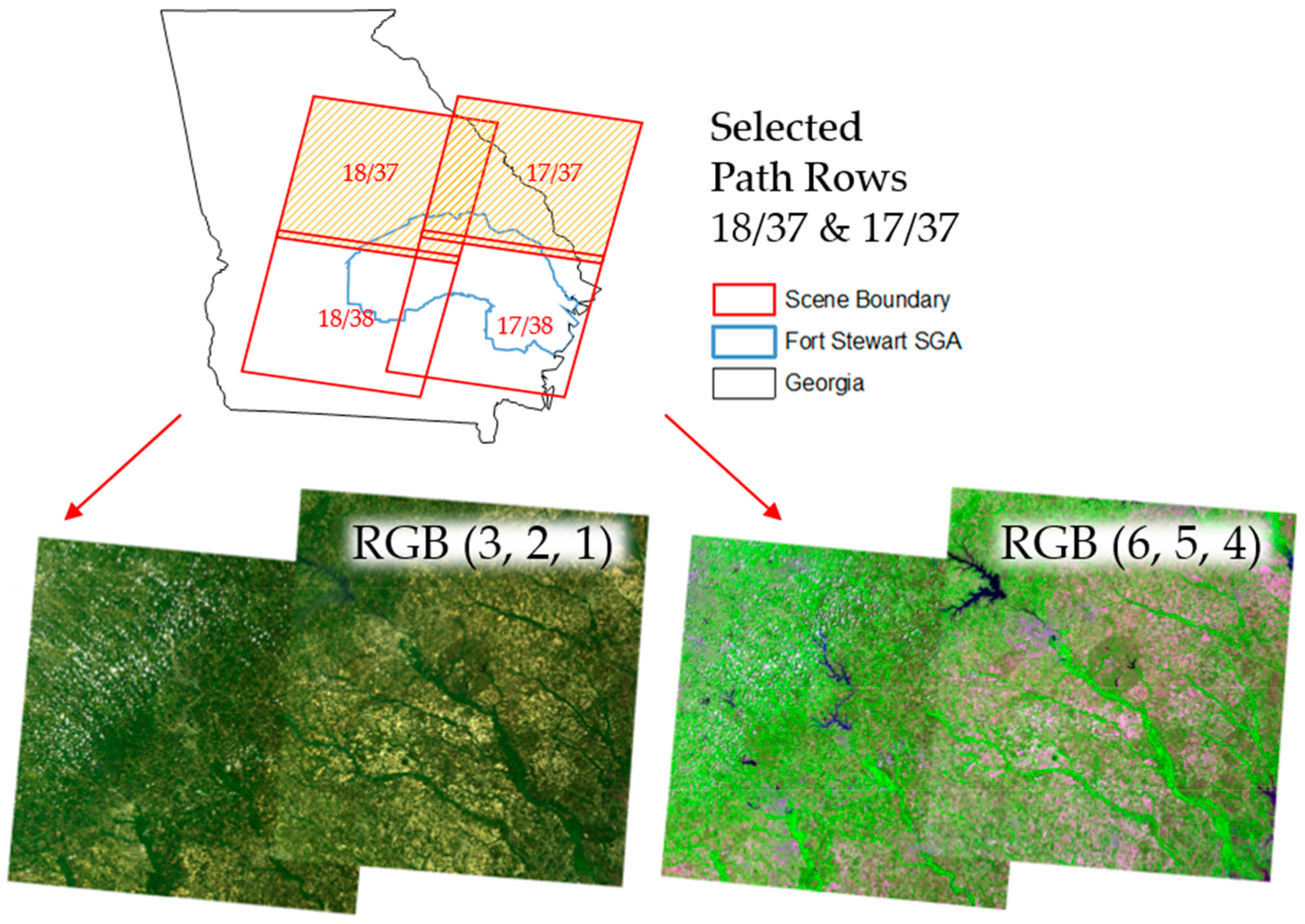
Figure 1.
Location, dates, path/row and mosaicking order of Landsat 8 imagery used in the study. Path/row 17/38 was used as the reference scene to relatively normalize scenes within a given phenology. The order in which images for a given phenology were mosaicked together is displayed in parentheses after path/row within the left most image.

Figure 2.
Example (red arrow) of scene striping in National Agriculture Imagery Program (NAIP) imagery caused by flight line scene boundaries displayed in color, color infrared (CIR) and individual bands within the Fort Stewart significant geographic area (SGA). Striping in the Blue and near infrared (NIR) bands is quite pronounced.

Figure 3.
Visual depiction of study methods. Step groupings identified by color in the figure correspond to named subsections.
Figure 3.
Visual depiction of study methods. Step groupings identified by color in the figure correspond to named subsections.

Figure 4.
Histograms and summary statistics of Forest Inventory and Analysis (FIA) plots for basal area per hectare (BAH) and trees per hectare (TPH) of needle-leaf (orange) and broadleaf (blue) species groups with and without zeros.
Figure 4.
Histograms and summary statistics of Forest Inventory and Analysis (FIA) plots for basal area per hectare (BAH) and trees per hectare (TPH) of needle-leaf (orange) and broadleaf (blue) species groups with and without zeros.

Figure 5.
Before aggregate no-change regression (ANR) normalization (left) and after ANR normalization (right) of Landsat 8 scenes for Leaf off, Growing and Dormant phylogenies. Bands 6, 5 and 4 are displayed here for the extent of the Fort Stewart study area (orange outline) as red, green and blue, color composites with a 2.5 standard deviation color stretch for each four scene mosaic. Pixel values for overlapping region within Landsat 8 images were calculated using the first image value given the order of the mosaicking process (Figure 1).

Figure 6.
Bootstrapped class frequency for L1 hard classifications. Each cell within a given accuracy assessment contains the mean number of occurrences (middle) and the lower (top) and upper (bottom) 95% confidence limits of occurrences given L1 models and a most likely class (MLC) rule. Overall map accuracies are presented in parentheses to the right of the contingency table name.

Figure 7.
Scatter plot of predicted (y-axis) vs observed (x-axis) values for basal area per ha (BAH) and trees per ha (TPH) hurdle models. Root mean squared error (RMSE) and bootstrapped estimates of lower and upper 95% RMSE confidence limits (within parentheses) are reported beneath each graphic’s title. The black dashed line and gray region surrounding that line depict the linear relationship and corresponding 95% confidence band between predicted and observed values. The solid red line is a one-to-one line and provides a benchmark for comparison.

Figure 8.
Graphic display of L1 and L2 outputs for the extent of the Fort Stewart SGA. Probability of dominant forest type (DomType) is displayed as a red, green and blue color composite. This rendering highlights dominant forest cover type probabilities as being either broadleaf (red), needle-leaf (green) or non-forested (blue). Presence of broadleaf (B_Leaf) and needle-leaf (N_Leaf) probability raster surfaces queried with a most likely class (MLC) rule were used to create the hurdle component of the basal area per ha (BAH) and trees per ha (TPH) raster surfaces. The probability of areas composed of predominantly young trees without a significant overstory component (Regen) and the presence of longleaf pine trees (L_Leaf) are displayed as black and white gradients. Combined within a geographical information system, these surfaces can be used to inform longleaf restoration.

Table 1.
The name, description, code, logical rules used to label each class (Query) and proportion of observations that makeup each class within each categorical response variable.
Table 1.
The name, description, code, logical rules used to label each class (Query) and proportion of observations that makeup each class within each categorical response variable.
| Name | Description | Code | Query 1 | Proportion |
|---|---|---|---|---|
| DomType * | Broadleaf | 1 | (B_BAH > N_BAH) AND NOT (TPHG < 20 AND TPHL < 556) | 0.38 |
| Needle-leaf | 2 | (N_BAH >= B_BAH) AND NOT (TPHG < 20 AND TPHL < 556) | 0.47 | |
| Non-forest | 3 | (TPHG < 20) AND (TPHL < 556) | 0.15 | |
| Regen | Regen | 1 | (DomType < 3) AND (TPHG < 49) AND (TPHL >741) | 0.07 |
| N_Leaf | Needle-leaf Presence | 1 | Needle-leaf BAH > 0 | 0.78 |
| B_Leaf | Broadleaf Presence | 1 | Broadleaf BAH > 0 | 0.83 |
| L_Leaf | Longleaf Presence | 1 | Longleaf BAH > 0 | 0.11 |
* 80 DomType observations were labeled from visual inspection of the NAIP imagery due to discrepancies between plot summaries and NAIP imagery.1 B_BAH = broadleaf basal area per hectare; N_BAH = needle-leaf basal area per hectare; TPHG = trees per hectare greater than or equal to 12.7 cm; and TPHL = trees per hectare less than 12.7 cm.
Table 2.
Model name, type, sample size and fit statistics for each model in the study.
| Model Name | Type | Sample Size | AIC 1/R 2 | Deviance 1/RSE | P-Value 2 |
|---|---|---|---|---|---|
| DomType | SoftMax | 762 | 878.644 | 794.644 | <0.001 |
| N_Leaf | SoftMax | 682 | 460.150 | 446.150 | <0.001 |
| B_Leaf | SoftMax | 682 | 418.850 | 408.850 | <0.001 |
| L_Leaf | SoftMax | 682 | 408.600 | 396.600 | <0.001 |
| Regen | SoftMax | 682 | 273.940 | 257.940 | <0.001 |
| N_BAH | Linear | 530 | 0.521 | 0.949 | <0.001 |
| N_TPH | Linear | 530 | 0.467 | 0.981 | <0.001 |
| B_BAH | Linear | 569 | 0.574 | 1.081 | <0.001 |
| B_TPH | Linear | 569 | 0.266 | 1.075 | <0.001 |
1 AIC and Deviance fit statistics apply to SoftMax models, while coefficient of determination (R2) and residual standard error (RSE) of transformed values apply to linear models. 2 P-values were calculated for chi-squared and F distributions for SoftMax and linear modeling techniques, respectively.
© 2019 by the authors. Licensee MDPI, Basel, Switzerland. This article is an open access article distributed under the terms and conditions of the Creative Commons Attribution (CC BY) license (http://creativecommons.org/licenses/by/4.0/).
Share and Cite
MDPI and ACS Style
Hogland, J.; Anderson, N.; Affleck, D.L.R.; St. Peter, J. Using Forest Inventory Data with Landsat 8 Imagery to Map Longleaf Pine Forest Characteristics in Georgia, USA. Remote Sens. 2019, 11, 1803. https://doi.org/10.3390/rs11151803
AMA Style
Hogland J, Anderson N, Affleck DLR, St. Peter J. Using Forest Inventory Data with Landsat 8 Imagery to Map Longleaf Pine Forest Characteristics in Georgia, USA. Remote Sensing. 2019; 11(15):1803. https://doi.org/10.3390/rs11151803
Chicago/Turabian StyleHogland, John, Nathaniel Anderson, David L. R. Affleck, and Joseph St. Peter. 2019. "Using Forest Inventory Data with Landsat 8 Imagery to Map Longleaf Pine Forest Characteristics in Georgia, USA" Remote Sensing 11, no. 15: 1803. https://doi.org/10.3390/rs11151803
Note that from the first issue of 2016, this journal uses article numbers instead of page numbers. See further details here.