Extraction of Power Line Pylons and Wires Using Airborne LiDAR Data at Different Height Levels


School of Information and Communication Technology, Griffith University, Nathan, QLD 4111, Australia
Remote Sens. 2019, 11(15), 1798; https://doi.org/10.3390/rs11151798
Submission received: 10 June 2019
/
Revised: 11 July 2019
/
Accepted: 31 July 2019
/
Published: 31 July 2019
(This article belongs to the Special Issue Remote Sensing: 10th Anniversary)
Abstract
:High density airborne point cloud data have become an important means for modelling and maintenance of power line corridors (PLCs). As the amount of data in a dense point cloud is large, even in a small area, automatic detection of pylon locations can offer a significant advantage by reducing the number of points that need to be processed in subsequent steps, i.e., the extraction of individual pylons and wires. However, the existing solutions mostly overlook this advantage by processing all of the available data at one time, which hinders their application to large datasets. Moreover, the presence of high vegetation and hilly terrain may challenge many of the existing methods, since vertically overlapping objects (e.g., trees and wires) may not be effectively segmented using a single height threshold. For extraction of pylons and wires, this paper proposes a novel approach which involves converting the input points at different height levels into binary masks. Long straight lines are extracted from these masks and convex hulls around the lines at individual height levels are used to form series of hulls across the height levels. The series of hulls are then projected onto a horizontal plane to form individual corridors. A number of height gaps, where there are no objects between the vegetation and the bottom-most wire, are then estimated. The height gaps along with the height levels consider the presence of hilly terrain as well as high vegetation within the PLCs. By using only the non-ground points within the extracted corridors and height gaps, the pylons are detected. The estimated height gaps are further exploited to define robust seed regions for the detected pylons. The seed regions thereafter are grown to extract the complete pylons. Finally, only the points between the locations of two successive pylons are used to extract points of individual wires. It first counts the number of wires within a power line span and, then, iteratively obtains individual wire points. When tested on two large Australian datasets, the proposed approach exhibited high object-based performance (correctness for pylons and wires of 100% and 99.6%, respectively) and high point-based performance (completeness for pylons and wires of 98.1% and 95%, respectively). Moreover, the planimetric accuracy for the detected pylons was 0.10 m. Thus, the proposed approach is demonstrated to be useful in effective extraction and modelling of pylons and wires.
1. Introduction
The reconstruction of an electrical power line corridor (PLC) is important in many applications including detection of potential hazards, such as vegetation encroachment [1] and analysis of power line (PL, wire) structural stability [2]. Traditionally, PLCs are surveyed in person or by manually inspecting aerial photos and videos. However, periodic inspection of thousands of kilometres of PLCs is not only time consuming and labour intensive, but also prone to error due to the involvement of human judgement.
The advent of airborne laser scanning technology, also known as LIght Detection And Ranging (LIDAR), now allows dense point cloud data to be collected which has made the survey more efficient and therefore more economic. Millions of 3D points on the Earth’s surface, both natural and structural, are collected and automatically processed off-line on powerful computers. A recent comprehensive review of various types of PLC surveying methods can be found in the work of Matikainen et al. [3].
The processing of LIDAR data for 3D mapping of PLC has two main steps [4]. Points are first classified or segmented into different objects such as trees, pylons, wires, and ground. Then, points on individual PL spans are exploited to model the wires strung between successive pylons. However, a good modelling of thin wire requires high density input data. There can, therefore, be millions of points in any given 1 km scene.
However, the actual number of points reflected from wires and pylons is far smaller than the number of input points. It is posited here that the detection of pylons in advance can make the wire extraction step faster as in this case only the non-ground points between successive pylons need to be processed. This prerequisite provides an important distinction within the extraction process. It might be noted here that parallel computing can also be used to extract wires from multiple spans simultaneously.
It should be noted that most of the existing PL extraction methods (e.g., McLaughlin [4]) overlook the detection of pylons as a pre-requisite for PL extraction, except that of Awrangjeb and Islam [5]. Sohn et al. [6] detected individual pylons, but did not use their location to help with the extraction of points for individual wires. Therefore, the advantage of exploiting pylon locations to reduce the workload and time for wire extraction is not realised and that process thus remains less economically efficient than the alternative proposed here.
In a vegetated area (e.g., forest) it might be possible for hundreds of trees to exhibit similar properties as pylons or other poles. Therefore, obtaining pylon locations as a pre-requisite for efficient wire extraction in a forest area can be a counter-productive step. This is clearly because the tree population will be so much greater than that of pylons and other poles that individual pylons/poles will not be identifiable in the data.
To circumvent this issue, the process needs to focus on the extraction of the actual PLCs from the input data before attempting the extraction of pylons. This two-step approach to extraction will help concentrate on the input points to those within the PLCs only thereby minimise the total amount of data that needs to be analysed for extraction purposes. It should be noted that in the literature there is no single method that explicitly extracts individual PLCs from the input data.
This paper presents a novel approach where PLCs, pylons and wires are extracted in order. PLCs are first extracted from the input point cloud data (Section 4.3). Each PLC consists of a set of rectangular regions that connect serially with each other to form a polygon which defines the parameters of the PLC. Then, only points within each rectangular PLC region are considered to locate and extract pylons (Section 4.4 and Section 4.5). Finally, the non-ground points between two successive pylons of the same PLC are used to extract individual wires (Section 4.6).
2. Related Work
This section briefly reviews the existing methods for pylon detection, pylon extraction, and wire extraction. While pylon “detection” refers to obtaining the positions of the individual pylons, pylon or wire “extraction” is the task of finding the points of each pylon or wire from the input LIDAR data.
2.1. Pylon Detection
Pylon detection techniques that provide individual pylon locations were proposed by Sohn et al. [6] and Awrangjeb and Islam [5]. Sohn et al. [6] first extracted 3D lines using the RANSAC (RANdom SAmple Consensus) algorithm. Then, these lines were converted into a binary image, from which 2D lines were classified using the Random Forest (RF) classifier based on the orientation and parallelism properties. Finally, non-pylon objects were removed using a voting scheme based on contextual relations among the lines. Using the non-ground points, Awrangjeb and Islam [5] first generated a PL mask, where successive pylons were found connected to each other by wires. They also generated a pylon mask within a specific low-height region where pylons were not connected with wires at all. The candidate pylons were then obtained using a connected component analysis on the pylon mask, followed by a removal of trees by comparing area, shape, and symmetry properties of trees and pylons. Finally, long lines representing wires were extracted from the PL mask and the parallelism property of these lines with the line connecting any pair of candidate pylons was validated to remove trees that had the same area and shape properties as pylons.
Both methods have shown 100% success rate in the detection of pylons. However, the application of Awrangjeb and Islam [5] to a complex forest dataset revealed that the method is not effective in extraction of pylons, since a common low height region cannot be found in a hilly terrain. Moreover, when trees exist within a corridor and underneath the wires, long straight lines that represent wires cannot be extracted effectively. As a result, both the pylon and PL mask become confusing and less useful for the intended purpose.
2.2. Pylon Extraction
Pylons are usually extracted as a separate class using “supervised classifiers”, e.g., RF [6,7] and JointBoost [2]. The classification output consists of a set of points for each class. Thus, 3D positions of individual pylons are usually not provided, except by the method of Sohn et al. [6]. Moreover, the supervised classifiers have two main requirements: a large training dataset and “balanced learning” [8]. A large training dataset for pylons is in general difficult to acquire for a given test scene. For example, the dataset used by Kim and Sohn [7] has only 0.81% points for pylons. Thus, pylons are in general a minority class compared to trees, buildings, and wires in any input datasets. Using such unbalanced classes of data, supervised classifiers tend to incorrectly classify minority classes [7].
2.3. Wire Extraction
Depending on how the input points are processed, the wire extraction methods can be categorised into two types: grid-based [9] and point-based [7] methods.
The grid-based methods interpolate the 3D point cloud data into a 2D grid space, where each grid cell (pixel) contains representative information such as point height or laser intensity values. They offer an effective way of managing a huge volume of point cloud data and take the advantage of easy application of various low-level computer vision algorithms like segmentation using region-growing techniques. However, these methods assume that each grid cell represents only one object, while vertically overlapped multiple objects may exist simultaneously within the same cell. For instance, 3D laser points returned from one of the following pairs of objects may exist in a single grid cell: wire and ground; vegetation and wire; and wire and pylon.
The point-based methods aim to extract (classify) individual objects considering every single point and they therefore carry out a full investigation of all 3D points to label each with an object class. The significant benefit of point-based methods is that vertically overlapped multiple objects can be labelled with different object classes, although the computational cost of such a full investigation is expensive.
The wire extraction methods in 3D point-based approach are further classified into three types based on how the input points are clustered or classified into individual objects in the scene [10]. Methods involving statistical analysis use height, density, and number of pulses [8,11,12]. Line-based wire extraction methods apply the Hough Transform (HT) [13,14,15] and RANSAC [16] algorithms to extract wires. Supervised classification-based methods first extract several features from the input data and then apply a classification algorithm [7,10,17]. As mentioned, line-based methods are computationally expensive for large datasets and incorrect topographic relationships may be established, especially when multiple objects overlap one another vertically. In contrast, the classification-based methods [18] require large training datasets, which are hard to collect, for desired results. In addition, an unbalanced sampling in the training set increases the rate of misclassification [8].
There are also hybrid methods that adopt two or more of the above approaches to cluster or classify points into individual objects in the scene. For example, Kim and Sohn [7] used the HT to extract lines and the RF for classification of points into five classes including wires and pylons. Axelsson [19] proposed a classification algorithm based on the minimum descriptor length criterion using the laser reflectance data and multiple echoes. The classification results were refined using the parallel and linear structures identified by the HT algorithm in the 2D grid space. Liu et al. [20] first separated ground points from the non-ground points using a statistical analysis. Then, to detect wires they applied an improved HT algorithm to the gridded non-ground data.
3. Contributions
This paper also presents a hybrid approach for extraction of pylons and wires. It adopts both the grid-based and point-based processing approaches of input data in order to leverage the benefits from both. In addition, it uses both statistical analysis and extracted lines in the process to extract pylons and wires. However, the proposed methodology does not use any supervised classifiers to avoid the shortcomings related to minority classes and unbalanced training datasets. The particular contributions are summarised as follows:
- To handle the presence of hilly terrain and vegetation within PLCs, a set of height thresholds is applied. In addition, for each PL segment a height gap, where there are no points except the pylon points, between the top-most point of the vegetation and the bottom-most point of the wires is estimated.
- The height thresholds and the height gap help locate individual pylons for extraction. To extract the pylons of various types and structures, a new “region growing” method based on a merging-diverging approach of individual pylon components is proposed.
- To extract individual wires between any two successive pylons, a new method to count the number of individual wires is first applied. Finally, for each wire a seed region is defined and, then, extended on both sides to extract the whole wire.
4. Proposed Methodology
Figure 1 shows the flow diagram of the proposed methodology. The input data consist of the LIDAR point cloud data and a Digital Terrain Model (DTM). The DTM with a resolution of 1 m has been supplied with the LIDAR data. It provides an approximate ground height for each given point in the LIDAR data. Thus, any height values used in the rest of the paper are presented as relative heights, calculated using the LIDAR data, from the ground.
A set of height levels (thresholds) are applied to generate binary masks, from where straight lines that mainly represent wires are extracted. The goal is to generate a range of heuristic height masks such that at some height level the trees will fall beneath. Convex hulls are formed around each cluster of parallel lines at each height level. Using the overlap among the hulls across successive height levels, series of hulls, which are used to estimate the height gap along a corridor, are obtained. The series of hulls is also used to extract PLCs in the form of 2D polygons.
The height gap indicates the vacant space that exists between the vegetation and the lowest point of the bottom-most wire. Only pylon points exist within the gap and therefore each pylon is located using the points within the gap. These points also serve as the seed for extraction of the pylon. The seed is grown downward first and, then, all its components are merged to get a complete cross-section of the pylon at a low height range. Finally, in the upward growth, the scaling of the pylon is considered to extract the whole pylon while considering possible diverging and connections through the cross arms.
At last, the points within each PL span (between the two successive pylons) are used to extract individual wires. The number of wires within the span is counted using two masks, specifically the vertical mask across the PL direction and the PL mask along the PL direction. “Bundle” wires, with up to two wires in each bundle, are correctly counted. For each wire, an initial wire segment is generated and extended towards both ends to get the points of the whole wire.
The overall idea of the proposed methodology is to reduce the number of input points that are processed in the subsequent steps. The extraction of PLCs help remove the vast amount of points that reside outside the corridors. Thus, only the non-ground points within the corridors are used to detect and extract pylons. Moreover, it is mainly the non-ground points above the height gap and between the successive pylons that are involved in the individual wire extraction process.
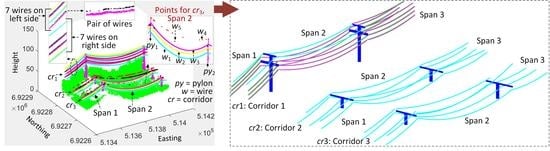
Figure 2a shows a data sample that will be used to demonstrate the details of the methodology.
4.1. Mask and Convex Hull Generation
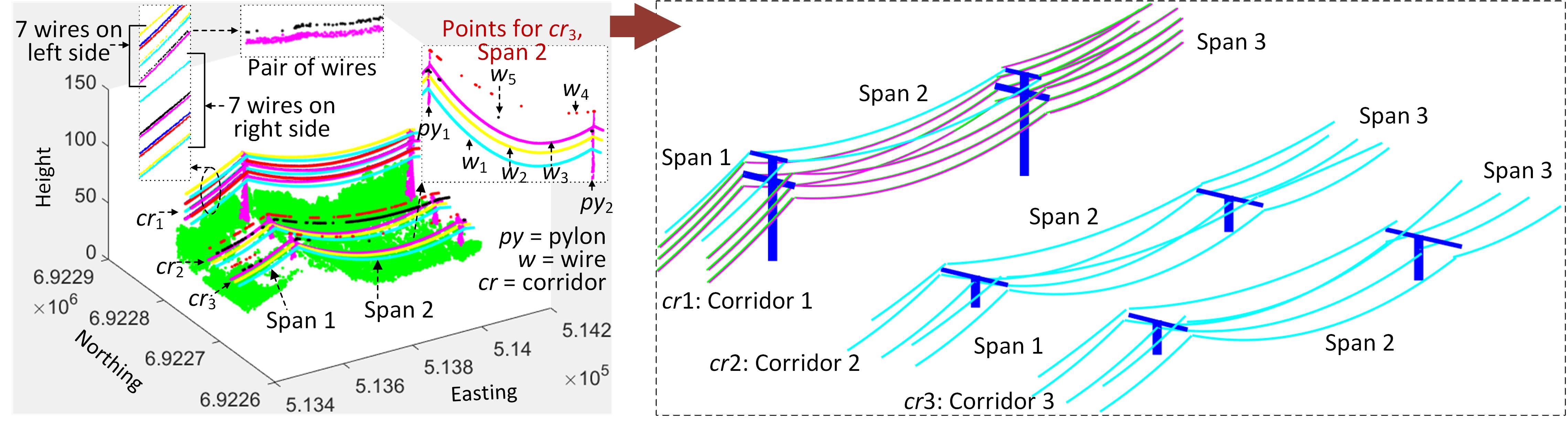
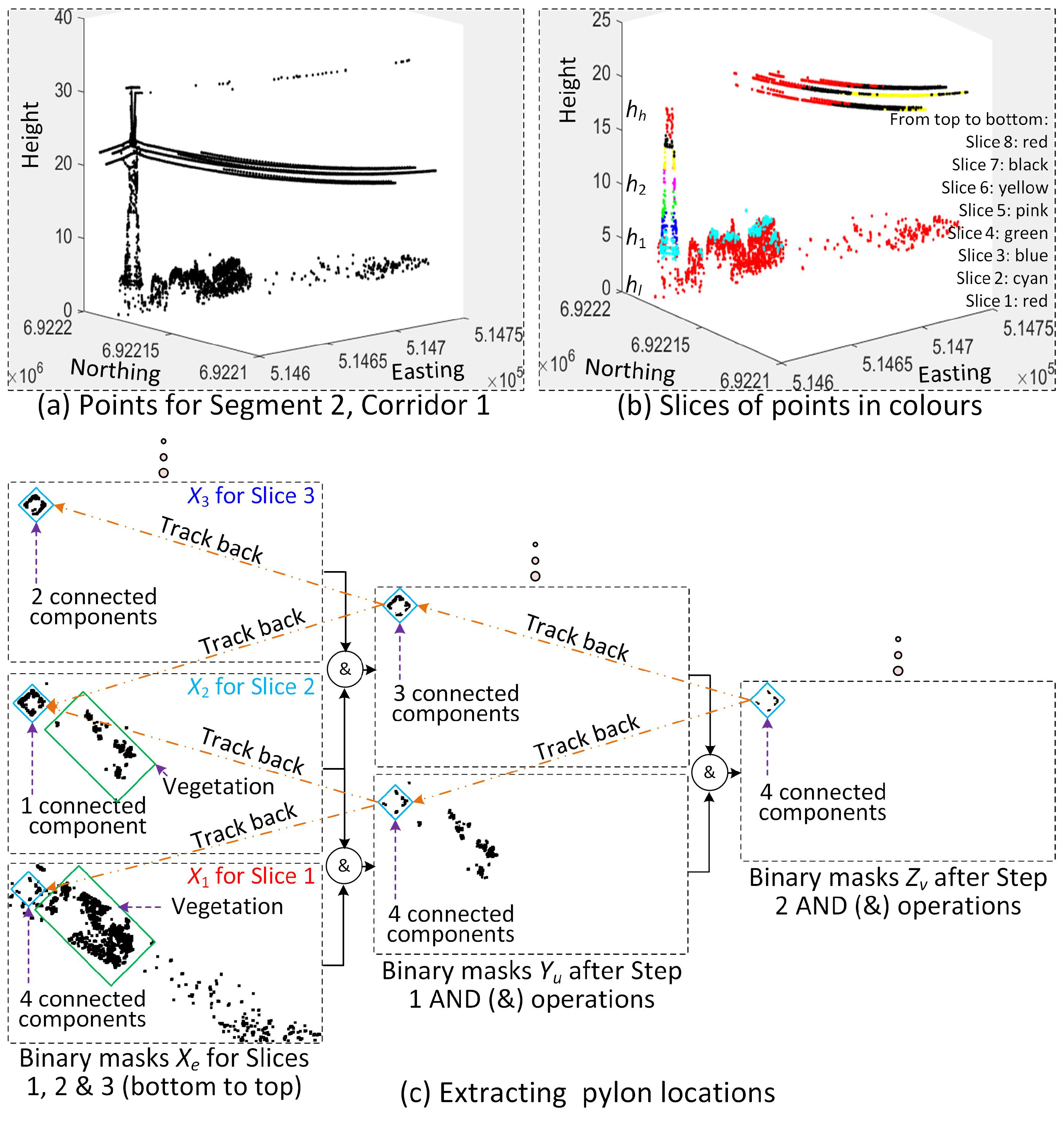
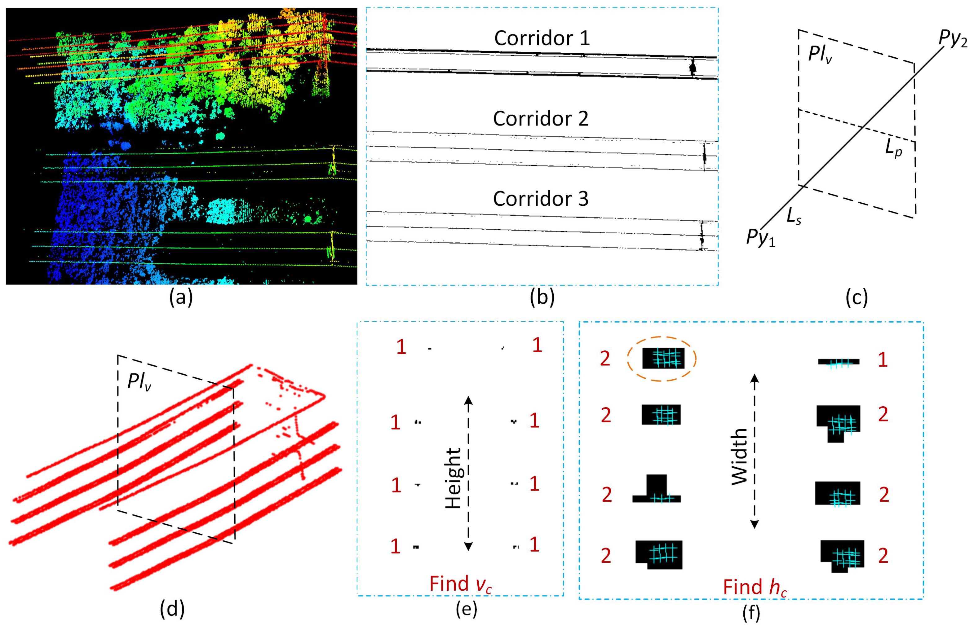
In the literature, other researchers have usually applied a height threshold h (e.g., m [10]) in order to separate ground and non-ground points. The non-ground points are expected to represent only desired objects such as pylons and wires. However, when there are tall trees below the PLs, as can be seen in Figure 2b, both trees and wires exist as non-ground points. For instance, Figure 2c shows the PL mask at m [5] indicating that vegetation exists in all three corridors, but especially in Corridor 3. Thus, a small value of h will not be effective to separate the expected objects from the unexpected objects. Moreover, in the same scene there can be multiple PLCs in which the pylons and wires exist at different heights. As a result, a single value of h may not work.
To overcome this issue, a set of height values m (relative to the ground) are used (see Figure 3). At every height level h, a PL mask is generated following the procedure presented in Awrangjeb and Islam [5]. Figure 2d–f shows generated for different h values. While Corridors 1 and 2 are obtained clearly at m, Corridor 3 is obtained at m. After its first clear appearance at a low h, a corridor may look identical for the next one or more h values. It may then start disappearing at a high h. This is because in the corridor there are wires at various heights. Each wire in a corridor can appear at different height levels (hence, in different masks) depending on the amount of sag in the wire and the height of the two connected pylons. When no wire points exist at a high h, the corridor completely disappears.
Consequently, at a given h, each corridor is either partially or fully extracted or completely missed. To combine them, straight lines , where , are extracted on each , again following the procedure of Awrangjeb et al. [21]. Figure 2g shows the extracted straight lines at . Assuming that wires between two consecutive pylons are longer than 6 m and the maximum width of a PLC is m, from each are organised into clusters of parallel lines. For each cluster, a convex hull , where , is finally generated using the end points of the lines. An axis that passes through the centre of is also obtained. The axis works as a representative for all lines within the cluster. Figure 2h–i shows the convex hulls and their axes in blue and pink, respectively.
4.2. Estimating The Height Gap
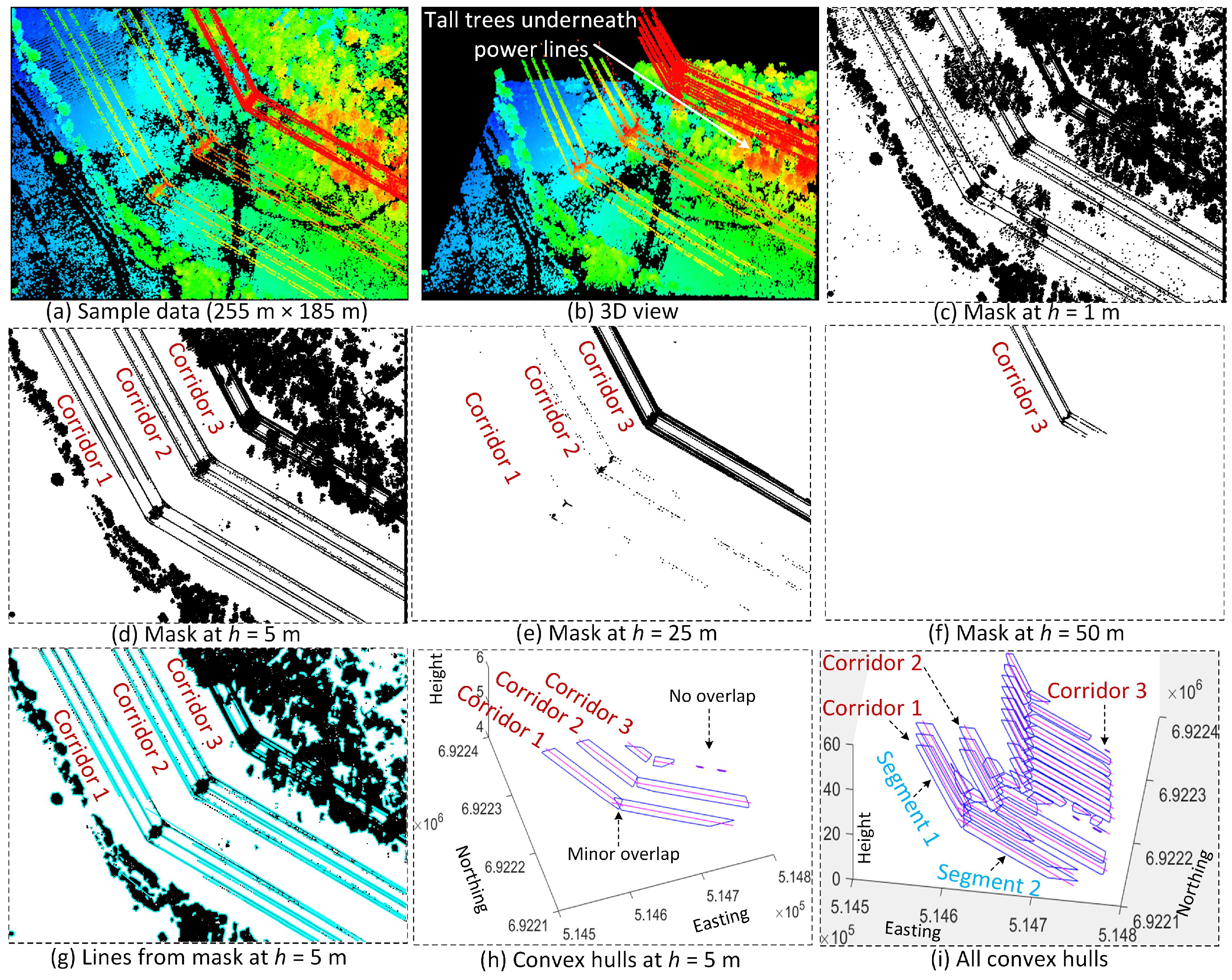
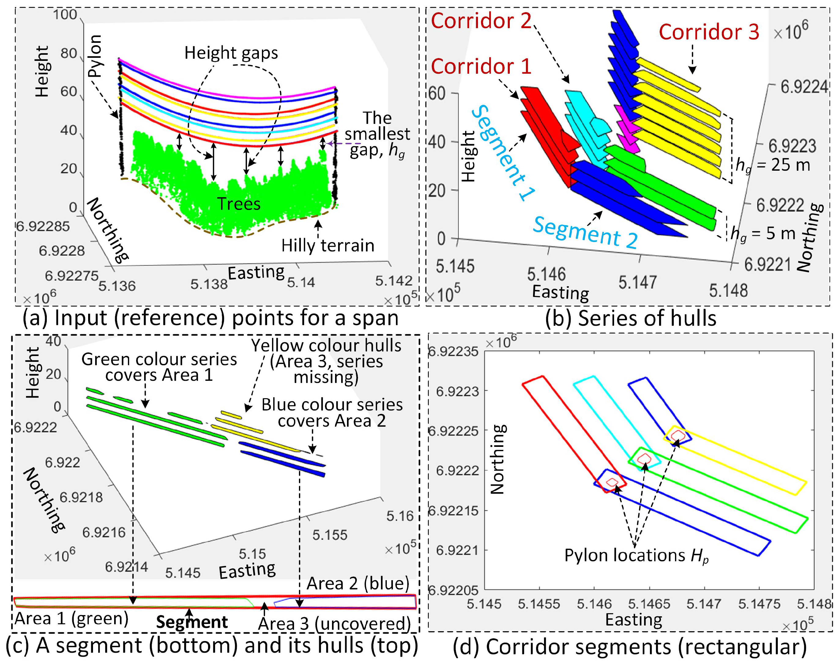
Figure 4a shows the input points between two pylons from the sample scene shown in Figure 2. Given that no vegetation (trees) touches any wires, a vertical height gap , where there are no points (except pylon points), always exists between the vegetation and the bottom-most wire. As mentioned above, the gap can vary along the span due to hilly terrain, vegetation height and the extent of sag in the wire. The smallest gap indicated in the figure is common to all variations. Ideally, therefore, it is this gap which must be estimated.
However, since the location of any two given pylons is unknown, the smallest cannot be estimated. Moreover, on the one hand an estimated value of for a span can be used for many other neighbouring spans along the same PLC. On the other hand, should any vegetation (trees) touch any wires within a span, there can be more than one value that needs to be estimated for that span. Thus, the purpose of the research presented herein is to attempt to estimate one or more such gaps within a straight PLC segment, which covers any number of spans of a PLC, using the convex hulls based on the observation below.
As shown in Figure 2i, convex hulls within a straight segment overlap one another vertically. If high vegetation does not exist underneath the wires, a large hull exists for each segment at a low h and it maximally overlaps the hulls at the next levels. However, as the height level increases, wire points completely disappear from the middle of some spans and there may be two or more hulls obtained for the same segment now. All four segments of Corridors 1 and 2 in Figure 2i reflect this fact. In contrast, if there are high trees underneath the wires then hulls are found to be small at low h. As h increases tree points gradually disappear and hulls merge and become larger. When no tree points exist at a high h, only a large hull exists within a segment and it maximally overlaps with the hulls at the next levels. The same trend is now displayed with the increase of h further when hulls become large in number but small in size. Two segments of Corridor 3 in Figure 2i illustrate this scenario.
Therefore, to estimate , a series , where , of hulls that largely overlap each other across neighbouring height levels are obtained (see Figure 5). Two hulls and are in if the two overlapping percentages (with respect to both hulls) are above the overlapping threshold (e.g., ). A series stops after the percentage with respect to does not satisfy the condition, i.e., seems to be smaller than . For the sample scene shown in Figure 2, Figure 4b shows the series of hulls in different colours. There is only one series covering each segment of Corridors 1 and 2. However, for the left hand side segment (Segment 1) of Corridor 3, there are two series (blue and pink). Since the pink series is short and completely contained within the blue series in a 2D top view, the former is ignored.
Ideally, one or more series covering a whole PLC are obtained as above. However, exceptions to this can happen when, for example, the vegetation between pylons grows as high as the wire is strung or where there is a considerable change in height in the wire. In these situations, convex hulls do not satisfy the above overlap condition and cannot be formed in some areas along a segment. To find these exceptions, all the current series are projected on a horizontal plane and checked if there are long gaps between consecutive series. Figure 4c shows a 1.285 km long segment (see the red polygon at the bottom; this segment is from a test dataset presented in Section 6.1), where two series cover two areas of the segment: Areas 1 and 2 are covered by the green and blue series. Both series are shown at the top of the figure. They are found at low height levels, e.g., m. However, because of high vegetation and hilly terrain, no hulls were extracted at these low height levels in Area 3, which is about 180 m long and situated between Areas 1 and 2. Hulls in this area were found at high height levels, e.g., m, as shown at the top of Figure 4c (yellow series). These hulls are not in any series obtained above, because their overlap percentages are below . To obtain these hulls in a series and, thereby, to fill up Area 3 in the segment, only hulls that cover a major part of the missing area (more than ) are considered. All the yellow hulls shown in Figure 4c satisfy this condition and, thus, form a series that covers Area 3 in the segment.
After having the entire series of hulls that completely cover each PLC, for a series , its height gap is recorded as [ ] and estimated as the difference in heights between the lowest and the second highest hulls. Figure 4b shows the estimated height values for two series of hulls: 25 m for yellow series ( m and m) and 5 m for green series ( m and m). This is a relative value with respect to the ground height provided by the DTM metadata, thus the actual value can be different at different locations.
4.3. Corridor Extraction
Each series of hulls is now used to define the minimum bounding rectangle that contains all of its hulls. Assuming that the maximum dimension of a pylon is m, this rectangle is extended about 10 m on both ends so that any two neighbouring rectangles (i.e., segments) clearly overlap each other. This overlap helps with retention of all the points of a pylon, which is in the intersection of two neighbouring segments, in both segments. Figure 4d shows that all corridor segments are now represented by such rectangles. If a segment has two or more such rectangles (e.g., three in Figure 4c), the segment is decomposed into the number of rectangles which represent the segment together. Each rectangle can be considered a “sub-segment”.
4.4. Detecting Pylons
To locate pylons, the area of each segment or sub-segment of a corridor is individually investigated (see Figure 6). Figure 7a shows the points for the right segment (blue) of Corridor 1 in Figure 4b. The estimated is 5 m, i.e., m and m for this segment.
Within , there are only points from the pylons, no points exist from either the vegetation or the wires. However, in practice, this gap can be too narrow (5 m in this case) to find enough points for pylon detection in low density input point data. Thus, based on the following observations, the gap is extended to and scrutinised after being divided into slices. Firstly, since pylons are usually wider at the bottom than at the top, there are more points reflected from the former than the latter. Thus, is set to have points above 1 m or more from the ground. Secondly, the sections of the wires nearest to the pylons are at a greater height than the sections of the wires further away from the pylon. Moreover, there may be no, or only a few, points in the short height of the pylon. Therefore, the height of each slice is set at m and is set. Given that the pylons in the test scenes are at least 20 m high, is set accordingly.
Figure 7b shows the points within height slices in different colours. A binary mask , where , is generated with points in each slice following the procedure of Awrangjeb and Islam [5]. The left side of Figure 7c shows three masks , and for Slices 1 (red), 2 (cyan) and 3 (blue), respectively, in Figure 7b. Given that pylons should extend upwards through all slices, and that vegetation does not continue after a certain height, the binary AND operation between masks of successive slices will preserve pylons, but remove vegetation. The binary masks in the middle and right sides of Figure 7c show the outcome of the two-step extraction process using AND operations: and after the Step 1 and Step 2 AND operations, where and .
It has also been observed that pylons always remain present either fully or partly in all binary masks, including after the AND operations. To remove high trees which exhibit similar properties of a pylon, a connected component analysis is carried out on all binary masks in , and . By verifying the common pixels, a double check is carried out for each component in . Firstly, a check is conducted on whether its related components exist in both and . If they do, then its related components are checked in previous levels by tracking back to and , respectively. The orange coloured dashed lines in Figure 7c show the tracking paths for a pylon in the sample test scene (i.e., only masks that created are checked in the tracking). Thereafter, all related components for each potential pylon are obtained in and a convex hull is formed around each set of all related components that reside close to one another. Figure 4d shows all three pylon locations (convex hulls, , where ) for the sample scene.
Note that the above pylon detection works fine based on the observation that for a true pylon there will be points in every slice. In contrast, for a tree, there may be no or a very few points that get reflected from some parts of its trunk. Thus, some slices at the bottom part of the tree will be (almost) empty. Thus, using the involved two-step AND operations while the pylon is detected, the tree is removed. However, if a tree has the same structure as a pylon (i.e., points get reflected from top to bottom of a tree), the algorithm may detect a false pylon.
4.5. Pylon Extraction
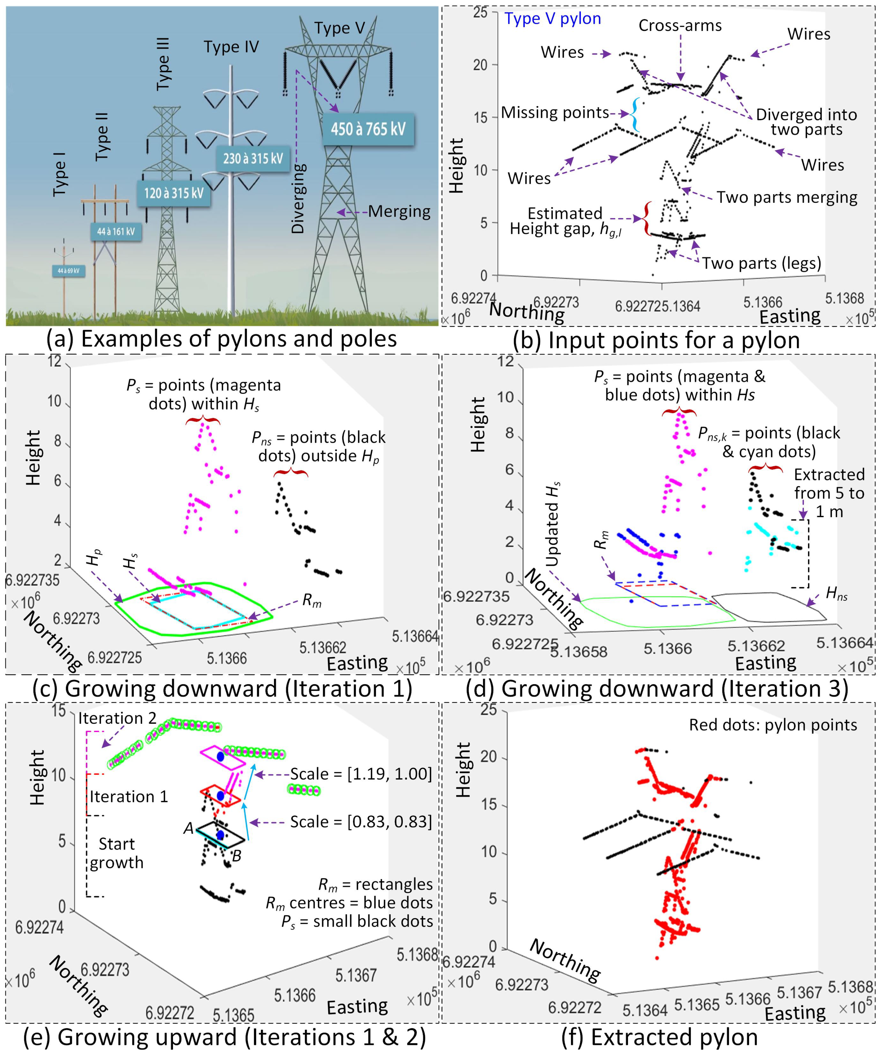
Electric pylons can be significantly different in both shape and structure. Figure 8a shows five types of pylon as provided by online (Hydro-Quebec, https://www.hydroquebec.com/securite/servitudes-droits-propriete/lignes-transport-postes-transformation.html (accessed on 10 June 2019).). Some of the obvious observations about pylons include: First, there can be more than one leg connected to the ground (Types II and V). Second, different parts or legs of the same pylon can be connected through cross arms (Type II) or merged into one (Type V). Third, a single pylon can be split (diverged) into two or more parts and then connected by cross arms (Type V). Fourth, there can be two or more pairs of cross arms at different heights (Types II and III). Last, the area of horizontal cross-section decreases with the increase of height (Types III and IV), except when the pylon diverges (Type V). An actual Type V pylon is shown in Figure 8b ( m). As can be seen, missing points are an almost regular phenomenon in the input point cloud data for both pylons and wires. As a result, a single component of a pylon can be found in two or more parts which makes the extraction of pylons a much more difficult task.
The proposed research here introduces a merging-diverging approach based on a connected component analysis (see Figure 9). The approach has three main steps: (1) select a seed region and grow pylon downward; (2) merge if two or more components of the same pylon are obtained in the downward growth; and (3) grow the pylon upward. The purpose of Steps 1 and 2 is to get a complete cross-section of the pylon at a low height range where the area of the cross-section is large. In Step 3, the scaling of the pylon is considered in order to extract the whole pylon while also considering all possible divergence and connections through cross arms. The pylon in Figure 8b is used below to describe the proposed procedure.
4.5.1. Growing Downward
For each pylon detected in Section 4.4, only points that reside within and the three consecutive slices above are considered as the seed. This avoids inclusion of any non-pylon points that may reside within the aforementioned extended height gap. For the pylon in Figure 8b,c shows the seed points (heights of 5–11 m) in magenta dots. A (convex) seed hull is obtained around . Considering that the pylon may have other parts (e.g., a second leg) outside , outside points within 1.5 m from the centroid of are also considered and designated as the non-seed points (black dots in Figure 8c), which may be merged with later.
To count the number of possible pylon parts and, thereby, to add points iteratively to the correct part, a connected component analysis is carried out at each iteration by converting the points into a binary mask. In practice, each of and may generate one or more components. All components generated by are combined into one to consider one pylon, but those generated by are considered individual non-seed components and are checked to determine whether any of them can be merged with . The convex hulls of the connected components are used to combine (within ) or form individual components (outside ).
Figure 10a shows each of and forms only one connected component in Iteration 1. Let the hulls of these components be and , respectively. By using the point-in-polygon test, all components within are found and a combined hull is obtained to update and . In our example, we have only within and, thus, is the updated seed hull. does not get updated since there are no points from close to . However, when there are points from that reside close to they may form a common component with some points in . In such a case, is updated with all previous points and new points from . Each of the remaining component hulls, which reside outside , needs to be preserved to track whether it continues in successive iterations. We have only one such hull (i.e., ), thus and all points within are assigned to , where .
The pylon is then grown downward iteratively, one slice at a time, and new points are added to and . New components may be found and existing components may disappear in any iterations. Figure 8d shows the points that are added in the next two iterations (slices at 5 to 3 and 3 to 1 m). Points added to are shown in blue, and those added to are shown in cyan. Figure 10b shows that there are still two non-overlapping components at Iteration 3 when the downward growth stops at the 1 m mark.
In addition, in each iteration, points in are used to generate a minimum bounding rectangle to track whether gets shrunk or enlarged in successive iterations. For example, the red dashed rectangle in Figure 8c is generated in Iteration 1. The updated in Iteration 3, shown in Figure 8d, is found enlarged, especially in the north direction. is used below to merge pylon components and to grow the pylon upward.
4.5.2. Merging
The downward growth of the pylon stops at the lowest slice (3 to 1 m). Before the pylon is grown upward, however, it needs to be investigated to determine whether any non-seed point sets can be merged with . To do that, slices above the current top slice (: 9–11 m in this case) are considered and points within each of these slices are scrutinised. Figure 10b shows the gap that exists between the two connected components generated by and (), respectively. If any points exist within the slices above , they can fill up the gap, which signifies can be merged with .
To investigate the possibility of merging the two minimum bounding rectangles and around and are shown in green and yellow, respectively. A combined bounding rectangle , shown in red, and has been calculated so that it includes and the gap between and . For each slice above the number of points are counted and if there are points within in a majority of slices (more than 50%), then is merged with . Figure 10c shows the points within from the higher height slices and the combined mask shows that the gap is now filled and only one connected component was obtained. In merging, points in are added to and is updated with the convex hull of the updated .
4.5.3. Growing Upward
While growing upward one slice at a time, starting from Slice , only points from the last three slices below are included into and is formed around . This is because the pylon being extracted may slowly shrink as in Types I–IV in and/or diverge as in Type V (see Figure 8a). In both cases, the current pylon in is only extracted upward and no new objects are added from outside . Considering only the last three slices (i.e., in 6 m height range) provides enough points to estimate the approximate cross-section of the pylon at a particular height range being examined.
To estimate the scaling factor , points within a new slice are checked to determine whether they are within or outside it (see Figure 10d). If all points are within , then the closest point from any side of is found and the intersection point between the line and the side is obtained, where is the centre of . Thus, . If there are points outside , the farthest outside point from any side of is obtained and , where is the intersection point between and the side. If there are no outside points but one or more points on , then .
It has been observed that, in practice, the area (i.e., horizontal cross-section) of a pylon changes slowly in successive slices. However, wire points can reside close to pylon points when they are at a similar height range. Thus, if there is a sudden change in (say, or higher) between successive slices, then the pylon is only enlarged across the corridor. This helps in not only excluding wire points from along the corridor but also helps to include pylon components such as insulators and cross arms. As shown in Figure 8a, cross arms and insulators are usually present across the corridor at high height and they enlarge (diverge) the area of a pylon’s cross-section.
Figure 8e shows the points from top three slices (5–11 m height) and their in black. The line indicates the direction across the corridor. In the first iteration, points within are shown in red and the updated is shrunk by the same factor on both directions (in and across the corridor direction). However, in the next iteration (magenta points), the pylon starts diverging and, thus, found enlarged only along . All the points outside and away from the pylon are shown in green circles. The extracted whole pylon is shown in red in Figure 8f.
4.6. Wire Extraction
Figure 11 shows the work flow of the proposed wire extraction technique. Before extraction of points on an individual wire, the number of wires within a PL span is counted. To count the number of wires, two binary masks are used. The first one is a vertical mask that shows the wires on a vertical cross section across the PL direction and helps find the clusters of wires at different height levels. The second one is the PL mask , which helps to count the number of wires that horizontally exists on each height cluster. Then, for each wire, an initial wire segment is generated. Finally, the initial segment is refined and extended towards both ends.
Note that the preliminary version of this wire extraction technique was published by Awrangjeb et al. [22]. In this submission, the technique is presented with further detail, particularly counting the number of wires and extracting the wire points. Figure 12a shows the input points for another sample scene, which is used below to explain the wire extraction technique.
4.6.1. Counting Wires in Masks
The 3D input points are converted to the 2D coordinate system of and a white mask is defined with a resolution . The width of is set to the width of the corridor and the height is set to cover the height difference between the lowest and highest points in the input. The value of is set to 0.15 m assuming that the transmission wires that vertically overlap each other have at least 1 m height difference. (see Figure 12b) is generated following the same procedure as for , but instead of a specific height h, a variable height is used from ().
Let be the pylon axis, i.e., the line connecting the mean points of two successive extracted pylons and and be the perpendicular line passing through the midpoint of (Figure 12c).
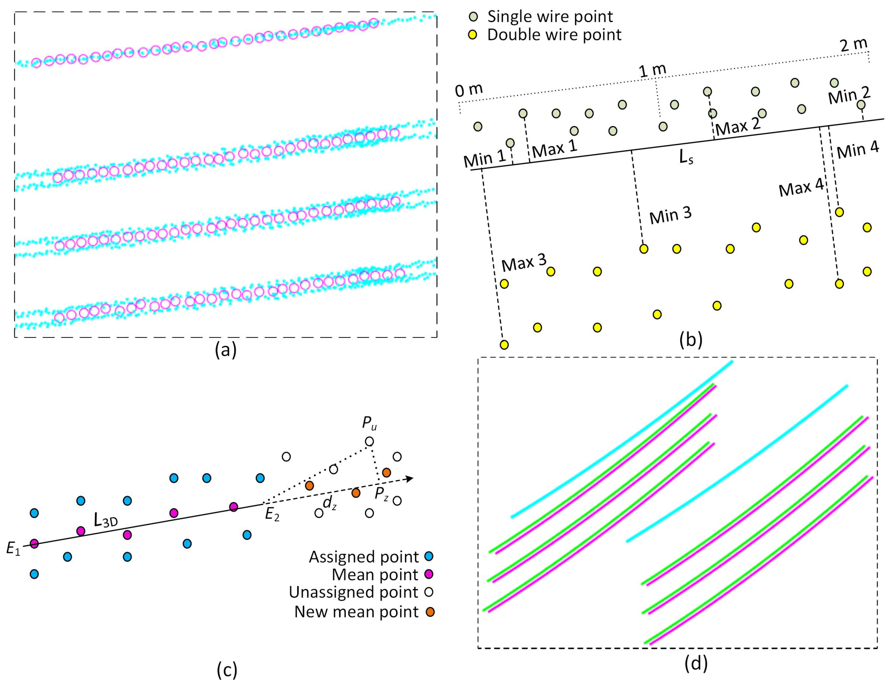
A vertical plane is generated passing through such that there are points on both sides of , as shown in Figure 12d. Starting from the nearest point on any side, the wire points within the next 1 m are taken and mapped into an empty . The wires are found as small individual black regions in and these are organised into clusters allowing a neighbourhood of 4 pixels (0.6 m) between any two black pixels in a cluster. This neighbourhood allows the wires in a particular bundle to be in the same cluster. Figure 12e shows eight clusters for in .
If a cluster is at most 2 pixels ( m) high (vertically), then the number of vertical wires is set for this cluster. Otherwise, , which does not happen since there are no vertically close wires in the test scene. Figure 12e shows that for all clusters is estimated correctly. To count the number of horizontal wires (across the PL direction), are now mapped into to capture the relevant wire parts, on which a connected component analysis is carried out. Figure 12f shows eight connected components, one for each cluster in Figure 12e. For each connected component, if the maximum width is 2 pixels then the number of horizontal wires is set for this component. Otherwise, , which usually happens for Corridor 1 since there are six pairs of wires and the wires in each pair are only about 0.30 m away from each other. Therefore, each pair are found in one connected component. The value of is mostly estimated correctly. However, sometimes it can be wrong, as shown within the orange coloured ellipse in Figure 12f. In , the single wire at the top left side of the corridor is confused with the double wires below it.
4.6.2. Extracting Initial Wire Segments
To find the actual values of and , the estimation of and continues iteratively as above, using 1 m of wire each time, running 30 times on the assumption that the maximum distance between two successive points on any wire is 30 m. The number of iterations is mainly set for thin wires (e.g., two single wires at the top of Figure 12d), which have a small number of points. It has also been found successful with thick wires as well (e.g., six pairs of wires at the bottom of Figure 12d).
At each iteration, all the points are marked as “assigned” and the mean point of is stored. Figure 13a shows the input points in cyan dots for seven wires (in front) at four height levels () and the mean points in magenta circles. We have four lists of mean points in this figure. In an iteration, to include a new mean point to a list of previously listed mean points, three checks are executed. First, and values are the same for both the list and . Second, the line connecting and the last mean in the list is parallel to the pylon axis . Third, the height difference between and is below a threshold ( m), which is calculated based on the distance between and and the tangent of the maximum possible slope of the wire. For parallelism and height checks, the angle threshold is set as .
4.6.3. Refining Initial Segments
Some of the wire segments extracted above may be spurious, containing only a small number of mean points. Thus, the segment with only one mean point is discarded. In addition, some of them may be the result of a split from a single wire. Therefore, every pair of the candidate segments is further scrutinised. Let and , where , be the set of mean points for two candidate segments m and n. Further, let and be two 3D lines of these two segments. The following check is performed to merge them, if possible. The perpendicular distances from to are within m and the height errors between the estimated and actual heights are within 0.5 m. If the check is true, then the longer segment is updated with the information of the shorter segment, which is abandoned thereafter.
After the above merging step, the value of is revised based on a majority voting criterion that uses the perpendicular distances from wire points to . Figure 13b shows one set of single wire (green) and one set of double wires (yellow) along a 2 m long segment. For both cases, the maximum and minimum perpendicular distances are shown in every 1 m space along . For the single wire, the difference between the maximum and minimum distances is less than m, therefore gets 1 vote for each 1 m segment. In contrast, for the double wires, the difference between the maximum and minimum distances is more than 0.3 m, therefore gets one vote for each group. After voting for all 1 m segments of a wire along , if gets the majority of votes, then this wire is decided as a single wire; otherwise, it is decided as a double wire.
4.6.4. Extracting Final Wires
Once the initial wire segments are refined as above, they are now extended according to the number of mean points . To avoid spurious wire extension, wires with the largest number of are extended first, then the second line with the largest number of , and so on. For each initial segment, it is extended on both sides iteratively, 1 m at a time. On each side, a 3D line is constructed using the last five mean points in that side of the wire. For a thin wire where we may not have many input points, a minimum of two mean points are still required to construct .
Figure 13c shows the “unassigned” points in black circles. are the intersection points between and the perpendicular lines from to . For each the height error is compared with a height threshold , which is estimated by considering the maximum slope of the wire and the distances from the nearest end of to : (see Figure 13c). For an unassigned point , it is assigned to the wire if . For all newly assigned points in an iteration, their mean is added to the wire segment. After each iteration, , and are updated considering the new mean point. Figure 13c shows the newly added three mean points in orange circles.
If, after the process for extraction of a wire is complete, it is decided as a double wire (), its mean points are used to divide all its “assigned” points into two wires. As evident from the bottom three pairs of wires in Figure 13a, the mean (magenta) points can be used to separate the (cyan) points into two wires. Otherwise, if it is a single wire (), it has only one wire, as can be evident from the top single wire in Figure 13a. Finally, each wire is modelled as a 3D polynomial curve [23] using the MATLAB polyfit function. Figure 13d shows the 3D wires for the input point cloud in Figure 12d. Six pairs of double wires are shown in green and magenta, while two single wires are shown in cyan.
5. Parameter Setting
Table 1 shows the list of parameters and their values used in the proposed approach. All of these parameters were first empirically set and tested for Bindebango dataset and, then, without resetting they were tested on Maindample dataset (see Figure 14 for these datasets) for independent performance evaluation.
Some of these parameters may not require any change at all for any new datasets. For example, the minimum wire length (i.e., the distance between successive pylons) is 6 m, which may be true for all transmission lines. The minimum height for non-ground points is 1 m which removes recognition of the low height vegetation and thus reduces the false pylon candidates. However, any new datasets which do not satisfy the other parameter values in Table 1 need to be reset accordingly. For instance, if the minimum pylon height is less than 20 m for an input dataset, it needs to be updated. The number of height slices also requires a re-estimation in this case since defines the seed region for pylon extraction.
The overlapping threshold value is not critical, because the approach proposes a procedure to search and fill the gap for any missing series of hulls (see Figure 4c). However, the height levels h, set in 5 m gaps (5 m, 10 m, 15 m, etc.), are critical. The main purpose of h is to generate masks using the non-ground points above these height levels such that some masks free of any vegetation within a PLC are obtained. A reduction in this gap will increase the number of levels and masks, thus the time consumption for corridor extraction will rise. However, an increase in the gap may not necessarily provide a benefit given that the overall number of masks free from vegetation within a PLC will be reduced. Moreover, this may make the estimation of impossible because series of vertically overlapping hulls will be reduced or completely absent.
The other parameters (e.g., , , etc.), which have been empirically set, are not sensitive to the performance of the proposed approach. To reduce execution time, the 3D line is updated in every five iterations on the assumption that a wire is locally (a 5 m long wire-segment for example) a straight line which can have a maximum slope of from the horizontal plane.
6. Performance Study
In this section, the test datasets, ground truth data, results, and discussion are presented in detail.
6.1. Datasets
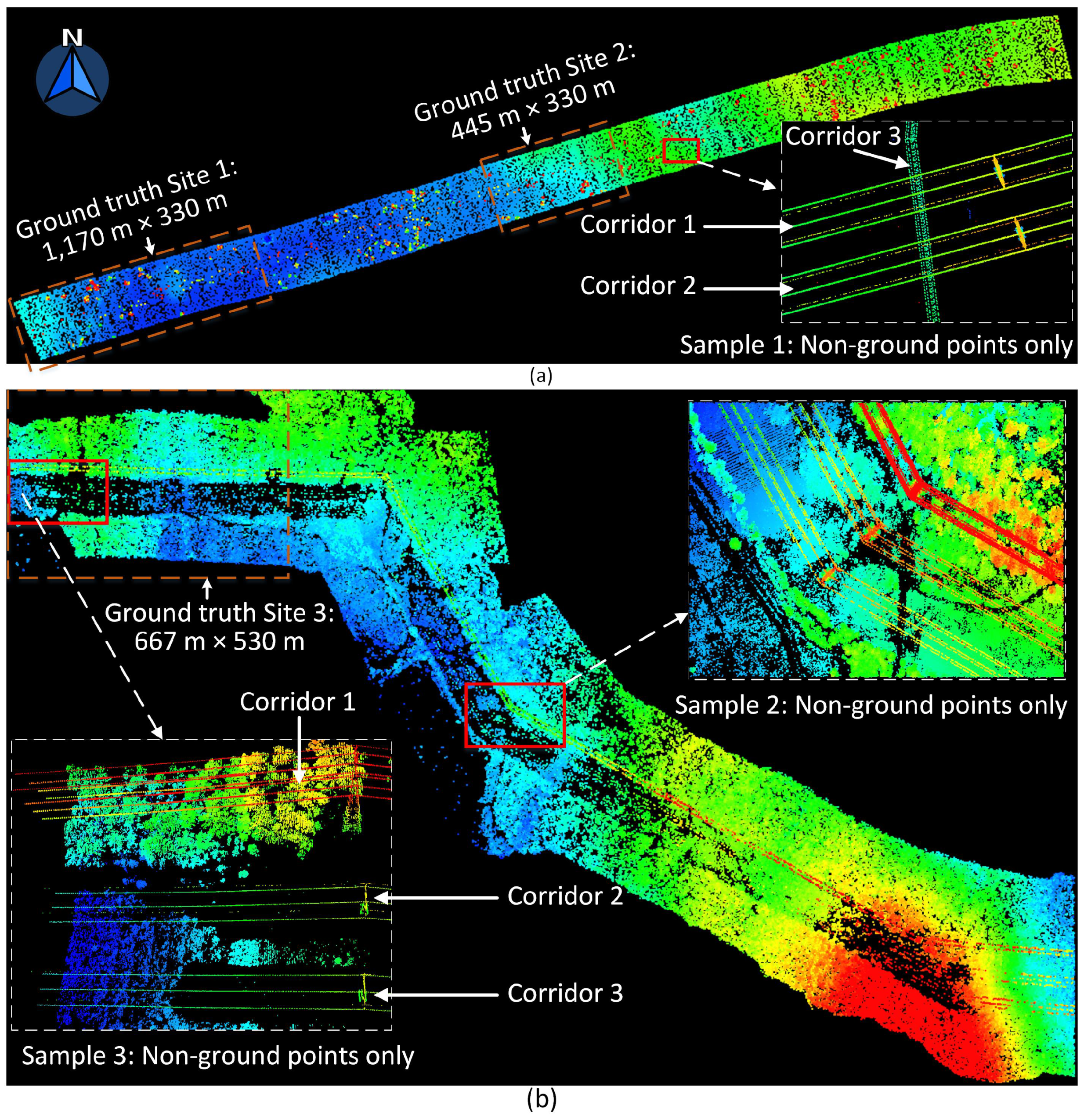
Figure 14 shows the two test datasets from Australia. Table 2 summarises the properties of these datasets. Both Bindebango and Maindample have three corridors and similar point densities. The length of Maindample is about twice the length of Bindebango, therefore the total number of points in the corridor is increased proportionally. While the width of Maindample is constant at 330 m, that of Bindebango varies between 330 m and 530 m. The third corridor of Maindample, as shown in Sample 1 of Figure 14a, is only 310 m long, intersects perpendicularly the other two corridors and passes underneath them. It has two “poles”, which are cylindrical columns. All other columns are “pylons” (26 in Maindample and 24 in Bindebango), which are columns made with steel frames. Note that the word “pylon” is used for both “pylon” and “pole” in this paper.
While Maindample is a flat area, Bindebango is a hilly area and there is dense vegetation underneath the wires, especially in Corridor 1 of Bindebango (see Sample 3 in Figure 14b). Therefore, the number of non-ground (NG) points as well as the number of NG within the corridors (NGC) is significantly higher in Bindebango (78.1% and 19.1%, respectively, of all points in the dataset) than those in Maindample (16.5% and 6.4%, respectively).
Sample 2 of Bindebango in Figure 14b shows that all the corridors significantly change their directions. A manual inspection of the input data shows that the number of wires in individual spans (i.e., pylon to pylon) of the three corridors varies: while for Corridor 1 there are from 14 to 16 wires, for Corridors 2 and 3 there are between 5 and 10 wires. For example, Sample 2 in Figure 14b shows that the fifth span in Corridor 1 has a total of 16 wires () at four height levels (), while each of Corridors 2 and 3 has eight wires ( + ) at two height levels (). Sample 3 in Figure 14b shows that the first span in Corridor 1 has a total of 14 wires () at four height levels (), while each of Corridors 2 and 3 has five wires () at two height levels (). The total number of wires in each corridor is shown within parenthesis in Table 2. In this counting method, even if a single point is found for a wire, it is assumed that a wire is present, while a maximum of two neighbouring wires (separated by a spacer) are considered at a height level.
In Maindample, all three corridors are almost straight. The number of wires in each corridor does not vary in this dataset. While Corridors 1 and 2 have eight wires () at two height levels (), Corridor 3 has six wires () at four height levels (). Note that, when two wires come in a pair, they are physically very close to each other: an approximate 0.3 m gap between them.
6.2. Ground Truth
The ground truth was not available for the two test datasets. A 3D interface was developed using MATLAB programming to manually collect the ground truth data. Since collecting the ground truth from the input points is difficult and time consuming, three sites were selected as shown in Figure 14. Table 3 shows the summary of the collected ground truth data. Points on the ground (height below 1 m) are not included at all. There are no other objects (e.g., buildings) other than wires, pylons and trees. The number of wires in Table 3 shows the total counts in all spans. For example, each span in Site 2 has eight wires, thus there are 16 wires altogether.
Figure 15a shows the ground truth data for Site 3. There are three corridors and two spans (Spans 1 and 2) in each corridor. The top-left snapshot shows 14 wires in Corridor 1 and Span 1 into two groups: left and right. The snapshot in the middle shows that points on a pair of wires that come together are very close to each other. The snapshot at the right shows the points on five wires for Corridor 3 and Span 2. As can be seen, while wires , and have dense points, has very sparse points and has only a few points. There are large gaps in between points in .
6.3. Evaluation Metrics
For performance evaluation, both object-based and point-based completeness, correctness and quality metrics [6] are employed. In object-based evaluation, the number of detected pylons as well as the number of extracted wires in all spans are considered. In point-based evaluation, the segmentation results are estimated against the ground truth presented above.
In addition, for pylons, a localisation error (in both 2D, i.e., planimetric, and 3D) is estimated as the distance between the two mean points of an extracted pylon and its corresponding ground truth data. For 3D wire models, a modelling error is estimated between the model generated from the extracted wire and the model generated from the corresponding ground truth data. The error is the difference between two distances and from each ground truth (wire) point to and , respectively.
6.4. Results and Discussions
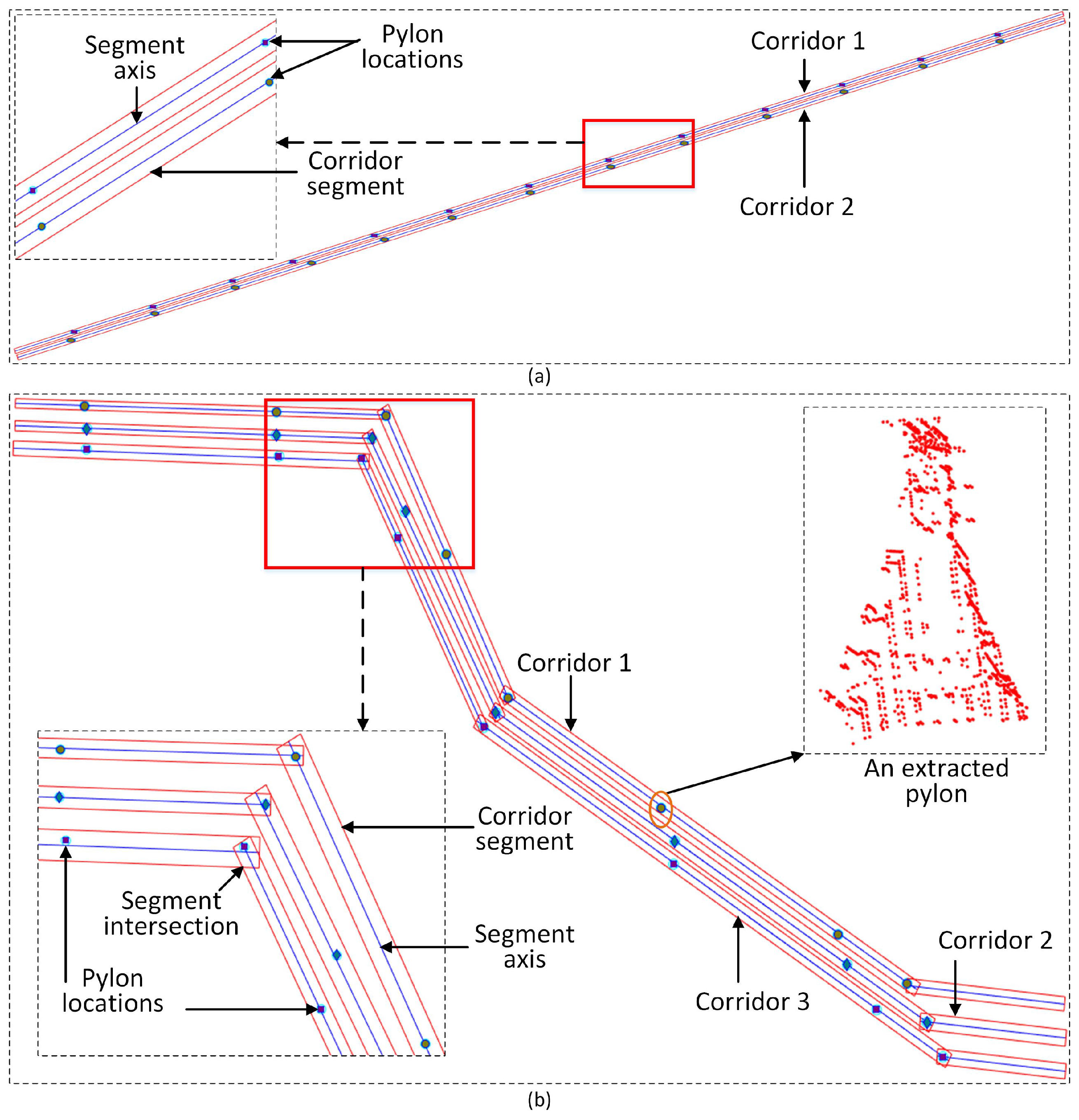
Figure 16 and Figure 17 show the extracted corridors, pylons and wires. Table 4 shows the object-based completeness, correctness and quality values for the whole datasets. All corridors in both datasets were extracted except Corridor 3 in Maindample (see Figure 14). This corridor is only 310 m long and 5.5 m wide. It is also situated underneath Corridors 1 and 2. Straight lines extracted along this corridor were short and broken (see Section 4.1). Therefore, the corridor and the two pylons (poles) there were missed. All other pylons (26 in Maindample and 24 in Bindebango) were correctly detected.
Although there are no incorrectly extracted corridors and pylons, there were some wires missed or incompletely extracted in both Maindample and Bindebango. Due to the missing corridor and pylons in Maindample, all 18 wires in Corridor 3 were missed. All 224 wires in Corridors 1 and 2 of Maindample were correctly extracted. The magnified version of Corridor 1, Span 2 in Figure 17a shows that there is no noticeable segmentation error in Maindample.
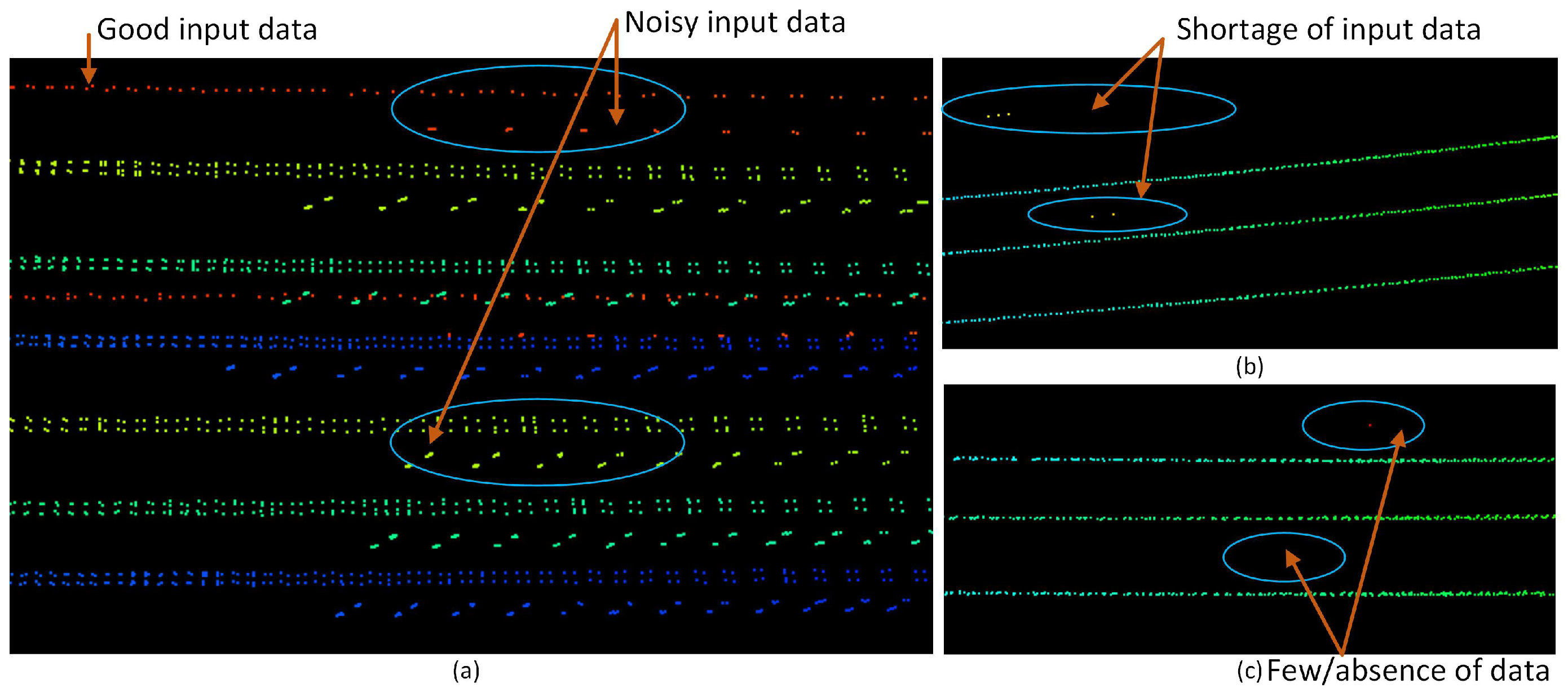
In Bindebango, the missing wires were due to the absence of data in some thin wires. Some wires were incorrectly extracted because of the presence of noise. The magnified version of Corridor 1, Span 2 in Figure 17b shows that sometimes there are gaps (segmentation error) due to noise in Bindebango. Figure 15b shows the wire models for the first three spans of all the three corridors in this dataset (for marked Region R in Figure 17b). For Corridor 1, despite the gaps due to segmentation errors, all 28 wires were correctly extracted and modelled in the first 2 spans; however, for the third span, the top two single wires were extracted as pairs because of the noisy input points. As shown in Figure 18a, within the top ellipse, clearly there are two rows of wire points captured for the single wire, which was why they were extracted and modelled as a pair of wires.
The same noisy data trend was observed for all double wires, e.g., for the double wires within the bottom ellipse, where there are four rows of data for two actual wires. Since the proposed method is only capable of obtaining double wires, it did not extract four wires here. Figure 18b shows the case where two top single wires are extracted correctly despite the shortage of the input points (i.e., where initial wire segments are found). However, in the case of extreme shortage of points (i.e., where no initial wire segments are found), the proposed algorithm cannot extract the wire at all (see Figure 18c).
Table 5 shows the point-based evaluation results against the ground truth presented in Table 3. Although the proposed approach does not classify trees, all unclassified non-ground points were considered as trees in the evaluation process due to the absence of any other objects (e.g., buildings) in the datasets. The “correctness” and “quality” values for trees were low in Sites 1 and 2, because these two sites are from Maindample, which has a very low vegetation coverage. Few wire and pylon points which remained unclassified were determined to be trees, resulting in low correctness and quality values for trees.
For pylons, the completeness and correctness were lower in Site 3 than those in Sites 1 and 2 because Site 3 consists of structurally different types and sizes of pylons. Moreover, there was dense vegetation around the pylons. Consequently, some pylon points were misclassified as trees. For wires, the completeness value was lower in Site 3 than that in Sites 1 and 2. The reason was that wire points close to pylon points were misclassified as pylons and vice versa.
In terms of the localisation error, the 3D errors were higher than the 2D (planimetric) errors in all sites, because the wire and vegetation points which were misclassified as pylon points added “high-height” errors. These errors could be negligible in practice given that pylons are generally placed at a distance from each other. While the modelling error in Sites 1 and 2 was very low, modelling errors for Site 3 were high. This was because of the noisy points in Site 3, as shown in Figure 18a.
7. Conclusions
This paper presents a new approach for extraction of corridors, pylons and wires. The newly-devised use of height levels provides the benefit of extracting vertically overlapping multiple objects (e.g., trees and wires). Therefore, the proposed approach is effective in forest and hilly areas as well as areas with a flat terrain. The proposed corridor extraction method is the first mention in the literature to the best of our knowledge. The approach outlined above significantly reduces the amount of data that need to be processed for extraction of pylons and wires. The newly proposed pylon detection technique successfully localises pylons, albeit with a small error allowance. The estimation of the height gap is new in the literature too. This process helps separate trees and wires. Moreover, the height gap facilitates defining the robust seed regions for effective extraction of pylon points. Finally, the iterative wire extraction method first counts the number of wires within a PL span and, then, obtains individual wire points. As demonstrated, when the approach was tested on two Australian datasets the proposed approach exhibited high object-based and point-based performance.
Nevertheless, the proposed approach has the following issues which need to be further investigated. First, it works when wires are present either individually or in pairs. It may not work effectively on bundle wires when three or more wires are present in a bundle. Second, for modelling an individual wire, its extracted points are used to estimate a 3D polynomial curve. A more realistic model could be obtained through adopting a catenary curve model [24]. In addition, the extracted pylons would be modelled [25]. Third, the estimation of the height gap is critical to the success of the proposed method. The proposed method now estimates a height gap for each series of hulls in a corridor assuming that there is a clear separation between the PL and trees underneath. However, when a series of hulls covers a long corridor segment, where there can be a hilly terrain and high vegetation that grows over the PL, a single estimated height gap may be ineffective. Thus, a better estimation of the height gap, especially a more local estimation that adapts to the local variation of the terrain as well as a vegetation encroachment, is paramount. Finally, the wire extraction method has been found less effective in the presence of noise in the data. Thus, a more robust wire extraction method is to be investigated taking into account the presence of noisy data.
Funding
The project was supported by Griffith University’s New Researcher Grant (036 Research Internal).
Acknowledgments
The authors would like to thank the AAM Group (www.aamgroup.com) for providing the test datasets.
Conflicts of Interest
The authors declare no conflict of interest.
Abbreviations
The following abbreviations are used in this manuscript:
| PLC | Power Line Corridor |
| PL | Power Line |
| LIDAR | LIght Detection And Ranging (LIDAR) |
| DTM | Digital Terrain Model |
| HT | Hough Transform |
| RANSAC | RANdom SAmple Consensus |
| RF | Random Forest |
References
- Ahmad, J.; Malik, A.S.; Xia, L.; Ashikin, N. Vegetation encroachment monitoring for transmission lines right-of-ways: A survey. ISPRS J. Photogramm. Remote Sens. 2013, 95, 339–352. [Google Scholar] [CrossRef]
- Guo, B.; Li, Q.; Huang, X.; Wang, C. An improved method for power-line reconstruction from point cloud data. Remote Sens. 2016, 8, 36. [Google Scholar] [CrossRef]
- Matikainen, L.; Lehtomaki, M.; Ahokas, E.; Hyyppä, J.; Karjalainen, M.; Jaakkola, A.; Kukko, A.; Heinonen, T. Remote sensing methods for power line corridor surveys. ISPRS J. Photogramm. Remote Sens. 2016, 19, 10–31. [Google Scholar] [CrossRef]
- McLaughlin, R.A. Extracting transmission lines from airborne LIDAR data. IEEE Geosci. Remote Sens. Lett. 2006, 3, 222–226. [Google Scholar] [CrossRef]
- Awrangjeb, M.; Islam, M.K. Classifier-free detection of power line pylons from point cloud data. ISPRS Ann. Photogramm. Remote Sens. Spatial Inf. Sci. 2017, 4, 81–87. [Google Scholar] [CrossRef]
- Sohn, G.; Jwa, Y.; Kim, H.B. Automatic powerline scene classification and reconstruction using airborne LIDAR data. ISPRS Ann. Photogramm. Remote Sens. Spat. Inf. Sci. 2012, 13, 167–172. [Google Scholar] [CrossRef]
- Kim, H.B.; Sohn, G. Point-based classification of power line corridor scene using random forests. Photogramm. Eng. Remote Sens. 2013, 79, 821–833. [Google Scholar] [CrossRef]
- Zhu, L.; Hyyppä, J. Fully-automated power line extraction from airborne laser scanning point clouds in forest areas. Remote Sens. 2014, 6, 11267–11282. [Google Scholar] [CrossRef]
- Clode, S.; Rottensteiner, F. Classification of trees and powerlines from medium resolution airborne laserscanner data in urban environments. In Proceedings of the APRS Workshop on Digital Image Computing, Brisbane, Australia, 21 February 2005. [Google Scholar]
- Wang, Y.; Chen, Q.; Liu, L.; Zheng, D.; Li, C.; Li, K. Supervised Classification of Power Lines from Airborne LiDAR Data in Urban Areas. Remote Sens. 2017, 9, 771. [Google Scholar] [CrossRef]
- Liang, J.; Zhang, J.; Deng, K.; Liu, Z.; Shi, Q. A New Power-Line Extraction Method Based on Airborne LiDAR Point Cloud Data. In Proceedings of the International Symposium on Image and Data Fusion, Tengchong, China, 9–11 August 2011. [Google Scholar]
- Ritter, M.; Benger, W. Reconstructing Power Cables From LIDAR Data Using Eigenvector Streamlines of the Point Distribution Tensor Field. In Proceedings of the International Conference in Central Europe on Computer Graphics, Visualization and Computer Vision, Plzen, Czech Republic, 25–28 June 2012; pp. 223–230. [Google Scholar]
- Jwa, Y.; Sohn, G.; Kim, H.B. Automatic 3D powerline reconstruction using airborne lidar data. Int. Arch. Photogramm. Remote Sens. Spat. Inf. Sci. 2009, 38, 105–110. [Google Scholar]
- Grigillo, D.; Ozvaldic, S.; Vrecko, A.; Fras, M.K. Extraction of power lines from airborne and terrestrial laser scanning data using the hough transform. Geodetski Vestnik 2015, 59, 246–261. [Google Scholar] [CrossRef]
- Yadav, M.; Chousalkar, C.G. Extraction of power lines using mobile LiDAR data of roadway environment. Remote Sens. Appl. Soc. Environ. 2017, 8, 258–265. [Google Scholar] [CrossRef]
- Melzer, T.; Briese, C. Extraction and Modeling of Power Lines from ALS Point Clouds. In Proceedings of the Workshop of the Austrian Association for Pattern Recognition, Hagenberg, Austria, 17–18 June 2004; pp. 47–54. [Google Scholar]
- Yang, J.; Kang, Z. Voxel-based extraction of transmission lines from airborne LiDAR point cloud data. IEEE J. Sel. Top. Appl. Earth Obs. Remote Sens. 2018, 11, 3892–3904. [Google Scholar] [CrossRef]
- Guo, B.; Huang, X.; Zhang, F.; Sohn, G. Classification of airborne laser scanning data using JointBoost. ISPRS J. Photogramm. Remote Sens. 2015, 100, 71–83. [Google Scholar] [CrossRef]
- Axelsson, P. Processing of laser scanner data–algorithms and applications. ISPRS J. Photogramm. Remote Sens. 1999, 54, 138–147. [Google Scholar] [CrossRef]
- Liu, Y.; Li, Z.; Hayward, R.; Walker, R.; Jin, H. Classification of Airborne LIDAR Intensity Data Using Statistical Analysis and Hough Transform with Application to Power Line Corridors. In Proceedings of the Digital Image Computing: Techniques and Applications, Melbourne, Australia, 1–3 December 2009; pp. 462–467. [Google Scholar]
- Awrangjeb, M.; Zhang, C.; Fraser, C.S. Automatic extraction of building roofs using LIDAR data and multispectral imagery. ISPRS J. Photogramm. Remote Sens. 2013, 83, 1–18. [Google Scholar] [CrossRef] [Green Version]
- Awrangjeb, M.; Gao, Y.; Lu, G. Classifier-Free Extraction of Power Line Wires from Point Cloud Data. In Proceedings of the Digital Image Computing: Techniques and Applications, Canberra, Australia, 10–13 December 2018; pp. 1–7. [Google Scholar]
- Qin, X.; Wu, G.; Ye, X.; Huang, L.; Lei, J. A novel method to reconstruct overhead high-voltage power lines using cable inspection robot LiDAR data. Remote Sens. 2017, 9, 753. [Google Scholar] [CrossRef]
- Jwa, Y.; Sohn, G. A Piecewise Catenary Curve Model Growing for 3D Power Line Rensostruction. Photogramm. Eng. Remote Sens. 2012, 78, 1227–1240. [Google Scholar] [CrossRef]
- Zhou, R.; Jiang, W.; Huang, W.; Xu, B.; Jiang, S. A heuristic method for power pylon reconstruction from airborne LiDAR data. Remote Sens. 2017, 9, 1172. [Google Scholar] [CrossRef]
Figure 1.
The flow diagram of the proposed methodology.

Figure 2.
Sample input data and PL masks at different height levels h.

Figure 3.
The work flow for generating masks and convex hulls.

Figure 4.
Estimating the height gap. Easting, Northing and Height are in metres (m).

Figure 5.
The work flow for estimating the height gap.

Figure 6.
The work flow for detecting pylon locations.

Figure 7.
Extraction of pylon locations. Easting, Northing and Height are in metres (m). Within the binary images in (c), black pixels indicate “true” and white pixels indicate “false” for any non-ground objects (i.e., pylon, tree, etc.).
Figure 7.
Extraction of pylon locations. Easting, Northing and Height are in metres (m). Within the binary images in (c), black pixels indicate “true” and white pixels indicate “false” for any non-ground objects (i.e., pylon, tree, etc.).

Figure 8.
Extraction of a pylon. Easting, Northing and Height are in metres (m). , pylon hull; , seed hull; , non-seed hull; and , the minimum bounding rectangle.
Figure 8.
Extraction of a pylon. Easting, Northing and Height are in metres (m). , pylon hull; , seed hull; , non-seed hull; and , the minimum bounding rectangle.

Figure 9.
The work flow for extracting pylon points.

Figure 10.
Binary masks of points in slices during pylon extraction: (a–c) Within the binary images, black pixels indicate “true” and white pixels indicate “false” for pylons; and (d) how to estimate scaling factor.
Figure 10.
Binary masks of points in slices during pylon extraction: (a–c) Within the binary images, black pixels indicate “true” and white pixels indicate “false” for pylons; and (d) how to estimate scaling factor.

Figure 11.
The work flow for extracting wire points.

Figure 12.
Counting the number of wires: (a) sample scene; (b) PL mask ; (c) corridor axis and vertical plane ; (d) input points between an end and a pylon of Corridor 1; (e) clusters of wires in vertical mask ; and (f) connected components from PL mask ( = perpendicular line to , = vertical count of wires and = horizontal count of wires).

Figure 13.
Wire extraction: (a) initial segments; (b) examining single and double wires; (c) extending an initial segment; and (d) 3D models for the sample scene in Figure 12d.
Figure 13.
Wire extraction: (a) initial segments; (b) examining single and double wires; (c) extending an initial segment; and (d) 3D models for the sample scene in Figure 12d.

Figure 14.
The test datasets: (a) Maindample, Victoria; and (b) Bindebango, Queensland. In the three samples, only the non-ground points with at least 1 m height above the ground are shown. Samples 2 and 3 are used in Figure 2 and Figure 12, respectively.

Figure 15.
(a) Ground truth data for Site 3 (see Figure 14); and (b) extracted wires from an extended area of Site 3.
Figure 15.
(a) Ground truth data for Site 3 (see Figure 14); and (b) extracted wires from an extended area of Site 3.

Figure 16.
Extracted corridors and pylon locations in the two test datasets: (a) Maindample; and (b) Bindebango.
Figure 16.
Extracted corridors and pylon locations in the two test datasets: (a) Maindample; and (b) Bindebango.

Figure 17.
Extracted pylons and wires in two test datasets (a) Maindample; and (b) Bindebango.

Figure 18.
Complex cases of noisy and missing data: (a–c) Regions A–C indicated in Figure 15b, respectively.
Figure 18.
Complex cases of noisy and missing data: (a–c) Regions A–C indicated in Figure 15b, respectively.


Table 1.
Parameter values used in the proposed approach.
| Parameters | Sections | Values | Sources |
|---|---|---|---|
| Minimum non-ground point height | Section 4.1 | 1 m | This paper |
| Height levels h | Section 4.1 | 5, 10, 15, … m | This paper |
| Minimum wire length | Section 4.1 | 6 m | This paper |
| Maximum corridor width | Section 4.1 | 20 m | Input data |
| Maximum pylon width | Section 4.3 | 10 m | Input data |
| The height gap | Section 4.2 | Variable | Estimated |
| Overlapping threshold | Section 4.2 | 70% | This paper |
| Minimum pylon height | Section 4.4 | 20 m | Input data |
| Height of a slice | Section 4.4 | 2 m | This paper |
| Number of height slices | Section 4.4 | 8 | Estimated |
| Neighbourhood for pylon parts | Section 4.5.1 | 1.5 | Estimated |
| Majority slices with points | Section 4.5.2 | 50% | This paper |
| Length of wires to consider in each iteration | Section 4.6 | 1 m | This paper |
| Vertical mask resolution | Section 4.6.1 | 0.15 m | This paper |
| Distance between vertically overlapped wires | Section 4.6.1 | 1 m | Input data |
| Neighbourhood for bundle wires | Section 4.6.1 | 4 pixels (0.6 m) | Estimated |
| Maximum height or width of a single wire (, ) | Section 4.6.1 | 2 pixels (0.3 m) | Estimated |
| Maximum height difference from point to wire | Section 4.6.2 | 1 m | This paper |
| Slope of wire | Section 4.6.2 | 22.5 | This paper |
| Maximum distance between points on a wire | Section 4.6.2 | 30 m | Input data |
| Maximum height error between actual and estimated | Section 4.6.2 | 0.5 m | This paper |
| Update 3D wire line in | Section 4.6.4 | 5 iterations | This paper |
Table 2.
Summary of the two Australian test datasets (NG, non-ground points; NGC, non-ground points within corridor; and CR, corridor).
Table 2.
Summary of the two Australian test datasets (NG, non-ground points; NGC, non-ground points within corridor; and CR, corridor).
| Data Sets | Area | Points () | Dimensions (m) | Number of Pylons | Number of Wires | ||||||||
|---|---|---|---|---|---|---|---|---|---|---|---|---|---|
| (m) | All | NG | NGC | CR 1 | CR 2 | CR 3 | CR 1 | CR 2 | CR 3 | CR 1 | CR 2 | CR 3 | |
| Maindample | 5560 × 330 | 32.7 | 2.1 | 0.3 | 5560 × 20 | 5560 × 20 | 310 × 5.5 | 13 | 13 | 2 | 8 (112) | 8 (112) | 6 (18) |
| Bindebango | 2500 × 430 | 18.5 | 14.5 | 3.5 | 3000 × 12 | 3000 × 18 | 3000 × 18 | 8 | 8 | 8 | 14–16 (136) | 5–10 (77) | 5–10 (74) |
Table 3.
Summary of the three ground truth sites (see Figure 14).
Table 3.
Summary of the three ground truth sites (see Figure 14).
| Sites | Area | Points | Total | |||||
|---|---|---|---|---|---|---|---|---|
| (m) | All | Wires | Pylons | Trees | Spans | Wires | Pylons | |
| Site 1 | 1170 × 330 | 56,515 | 50,679 | 5001 | 835 | 6 | 48 | 6 |
| Site 2 | 445 × 330 | 24,317 | 19,634 | 3517 | 1166 | 2 | 16 | 4 |
| Site 3 | 667 × 530 | 435,579 | 36,062 | 3860 | 395,657 | 6 | 48 | 6 |
| Total | 886,460 | 516,411 | 106,375 | 12,378 | 397,658 | 14 | 112 | 16 |
Table 4.
Object-based evaluation on the whole datasets (all values are in percentage).
| Data Sets | Corridors | Pylons | Wires | ||||||
|---|---|---|---|---|---|---|---|---|---|
| Comp. | Corr. | Qual. | Comp. | Corr. | Qual. | Comp. | Corr. | Qual. | |
| Maindample | 66.7 | 100 | 66.7 | 92.9 | 100 | 92.9 | 92.6 | 100 | 92.6 |
| Bindebango | 100 | 100 | 100 | 100 | 100 | 100 | 92.6 | 99.2 | 91.9 |
| Average | 83.4 | 100 | 83.4 | 96.5 | 100 | 96.5 | 92.6 | 99.6 | 92.3 |
Table 5.
Point-based evaluation on the three sites against the ground truth presented in Table 3 (completeness, correctness and quality are in percentage; localisation error for pylons and modelling error for wires are in metres).
Table 5.
Point-based evaluation on the three sites against the ground truth presented in Table 3 (completeness, correctness and quality are in percentage; localisation error for pylons and modelling error for wires are in metres).
| Sites | Trees | Pylons | Wires | |||||||||
|---|---|---|---|---|---|---|---|---|---|---|---|---|
| Comp. | Corr. | Qual. | Comp. | Corr. | Qual. | (2D) | (3D) | Comp. | Corr. | Qual. | ||
| Site 1 | 100 | 73.2 | 73.2 | 99.1 | 98.1 | 97.2 | 0.14 | 0.25 | 99.3 | 100 | 99.2 | 0.00061 |
| Site 2 | 100 | 86 | 86 | 99.3 | 97.5 | 96.8 | 0.03 | 0.18 | 98.7 | 100 | 98.7 | 0.00029 |
| Site 3 | 100 | 98.8 | 98.8 | 95.9 | 96.1 | 92.3 | 0.14 | 0.59 | 86.9 | 100 | 86.8 | 0.04244 |
| Average | 100 | 86 | 86 | 98.1 | 97.2 | 95.4 | 0.10 | 0.34 | 95 | 100 | 94.9 | 0.01444 |
© 2019 by the author. Licensee MDPI, Basel, Switzerland. This article is an open access article distributed under the terms and conditions of the Creative Commons Attribution (CC BY) license (http://creativecommons.org/licenses/by/4.0/).
Share and Cite
MDPI and ACS Style
Awrangjeb, M. Extraction of Power Line Pylons and Wires Using Airborne LiDAR Data at Different Height Levels. Remote Sens. 2019, 11, 1798. https://doi.org/10.3390/rs11151798
AMA Style
Awrangjeb M. Extraction of Power Line Pylons and Wires Using Airborne LiDAR Data at Different Height Levels. Remote Sensing. 2019; 11(15):1798. https://doi.org/10.3390/rs11151798
Chicago/Turabian StyleAwrangjeb, Mohammad. 2019. "Extraction of Power Line Pylons and Wires Using Airborne LiDAR Data at Different Height Levels" Remote Sensing 11, no. 15: 1798. https://doi.org/10.3390/rs11151798
Note that from the first issue of 2016, this journal uses article numbers instead of page numbers. See further details here.