Mapping Paddy Rice Planting Area in Northeastern China Using Spatiotemporal Data Fusion and Phenology-Based Method


1
Institute of Remote Sensing and GIS, Peking University, No. 5 Yiheyuan Road, Haidian District, Beijing 100871, China
2
Beijing Laboratory of Water Security, Base of the State Key Laboratory of Urban Environment Process & Digital Modeling, Capital Normal University, Beijing 100089, China
3
Engineering Research Center of Earth Observation and Navigation (CEON), Ministry of Education of the People’s Republic of China, Beijing 100871, China
*
Author to whom correspondence should be addressed.
Remote Sens. 2019, 11(14), 1699; https://doi.org/10.3390/rs11141699
Submission received: 16 May 2019
/
Revised: 14 July 2019
/
Accepted: 16 July 2019
/
Published: 18 July 2019
(This article belongs to the Special Issue Advances of Multi-Temporal Remote Sensing in Vegetation and Agriculture Research)
Abstract
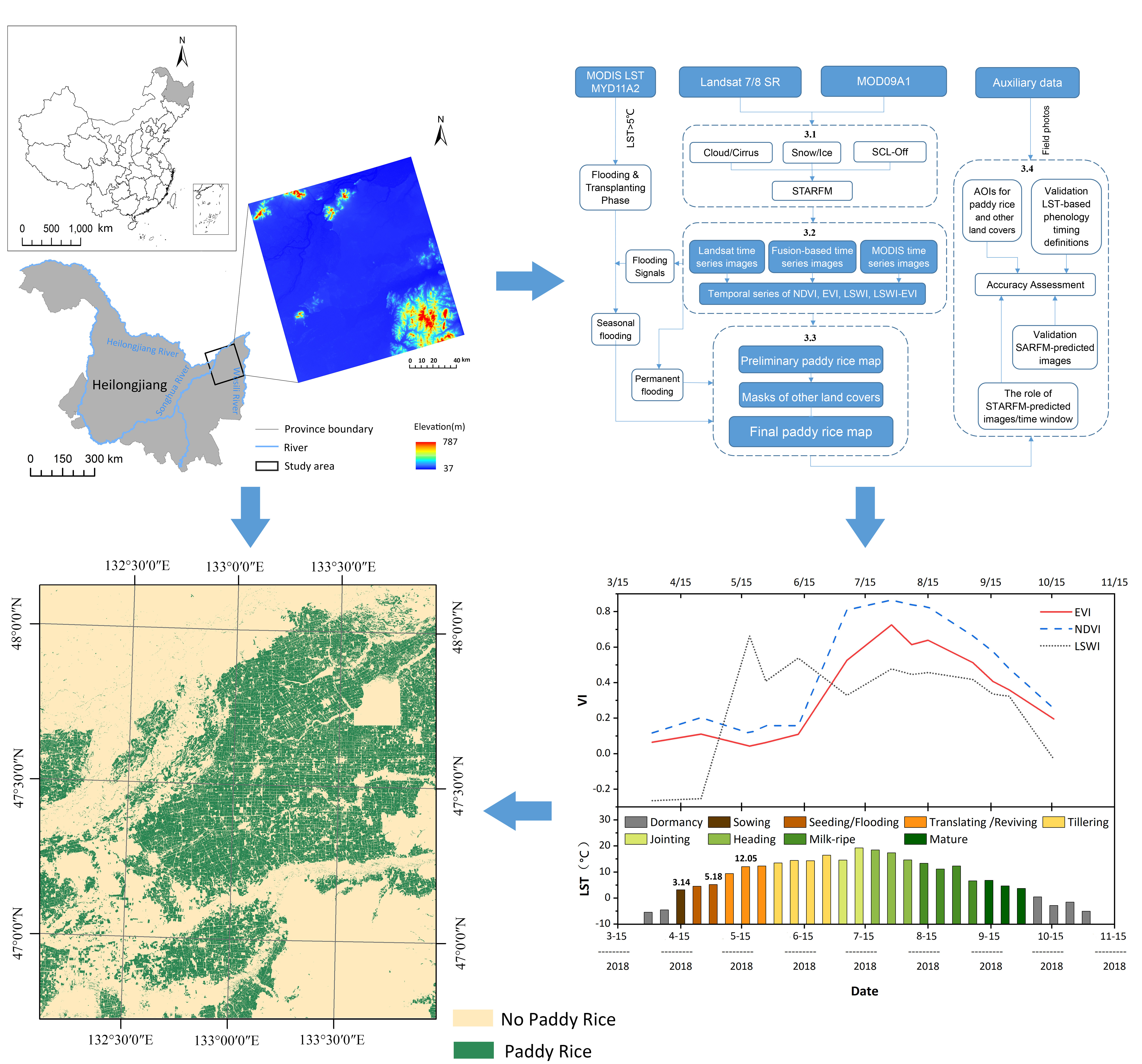
:Accurate paddy rice mapping with fine spatial detail is significant for ensuring food security and maintaining sustainable environmental development. In northeastern China, rice is planted in fragmented and patchy fields and its production has reached over 10% of the total amount of rice production in China, which has brought the increasing need for updated paddy rice maps in the region. Existing methods for mapping paddy rice are often based on remote sensing techniques by using optical images. However, it is difficult to obtain high quality time series remote sensing data due to the frequent cloud cover in rice planting area and low temporal sampling frequency of satellite imagery. Therefore, paddy rice maps are often developed using few Landsat or time series MODIS images, which has limited the accuracy of paddy rice mapping. To overcome these limitations, we presented a new strategy by integrating a spatiotemporal fusion algorithm and phenology-based algorithm to map paddy rice fields. First, we applied the spatial and temporal adaptive reflectance fusion model (STARFM) to fuse the Landsat and MODIS data and obtain multi-temporal Landsat-like images. From the fused Landsat-like images and the original Landsat images, we derived time series vegetation indices (VIs) with high temporal and high spatial resolution. Then, the phenology-based algorithm, considering the unique physical features of paddy rice during the flooding and transplanting phases/open-canopy period, was used to map paddy rice fields. In order to prove the effectiveness of the proposed strategy, we compared our results with those from other three classification strategies: (1) phenology-based classification based on original Landsat images only, (2) phenology-based classification based on original MODIS images only and (3) random forest (RF) classification based on both Landsat and Landsat-like images. The validation experiments indicate that our fusion-and phenology-based strategy could improve the overall accuracy of classification by 6.07% (from 92.12% to 98.19%) compared to using Landsat data only, and 8.96% (from 89.23% to 98.19%) compared to using MODIS data, and 4.66% (from93.53% to 98.19%) compared to using the RF algorithm. The results show that our new strategy, by integrating the spatiotemporal fusion algorithm and phenology-based algorithm, can provide an effective and robust approach to map paddy rice fields in regions with limited available images, as well as the areas with patchy and fragmented fields.

1. Introduction
Rice is one of the major staple foods worldwide and plays an essential role in supporting the growing population. Timely and efficient monitoring of paddy rice fields is a prerequisite for paddy rice growth monitoring, yield estimation, and agricultural resource management. In recent decades, paddy rice fields have expanded rapidly due to increasing population and food demand, especially in northeastern China [1,2], which is exerting pressures on cultivated lands, regional biodiversity and water resources. Monitoring the spatiotemporal dynamics of paddy rice fields is of great significance to food safety [3], water resources management [4], and ecosystem sustainability [5].
The rapid development of satellite remote sensing technology has greatly improved our ability to observe, monitor, and map paddy rice fields [6]. Compared to single time imagery used in traditional classification, time series imagery can provide more temporal information and help capture phenology information, thereby reducing the classification errors [7]. In recent years, phenology-based algorithms have been developed. For example, Zhang et al., 2017 successfully used MODIS LST product to define rice flooding/transplanting period, and then used MODIS-derived VI temporal profiles to analyze the spatiotemporal patterns of paddy rice fields from 2000 to 2015 [8]. Zhou et al., 2016 used the phenology-based method through analysis of Landsat and MODIS images to extract the paddy rice planting area from the rice-wetland coexistent area [9]. These algorithms extract phenology information and recognize the key phenology phase (e.g., flooding and transplanting phase, tillering) using spectral reflectance or vegetation indices at individual pixels from time series imagery.
The most representative phenology-based paddy rice mapping method is the transplanting-based algorithm [8]. Paddy rice fields are a mixture of water and rice plants in the flooding and transplanting phase and thus have unique physical characteristics. This feature can be detected based on the relationship between the time series Land Surface Water Index (LSWI) [10] and Normalized Difference Vegetation Index (NDVI) [11] or Enhanced Vegetation Index (EVI) [12]. At present, the transplanting-based algorithm has been widely used for rice field mapping in many regions [7,13,14,15]. For example, Xiao et al. successfully applied the transplanting-based algorithm to paddy rice mapping and generated rice distribution maps in South China, South Asia and Southeast Asia based on MODIS data [13,16]. Zhang et al. obtained the paddy rice map of northeastern China in 2010 by using time series MODIS-derived VI data [17].
At present, MODIS data has been widely used in the transplanting-based algorithm to map paddy rice for its high revisit frequency [18]. However, its coarse spatial resolution (250 m–1 km) limits its suitability in monitoring small cropland patches with high spatial complexity. Especially in China where paddy rice is usually planted in small, patchy and fragmented fields, the low spatial resolution of MODIS imagery makes it extremely difficult to generate accurate paddy rice mapping [8]. The Landsat imagery is an alternative data source with 30 m spatial resolution [6]. However, because of its low temporal resolution (16 days), it is difficult to obtain enough cloud-free Landsat images for time series analysis. Therefore, neither the MODIS nor the Landsat alone is suitable for mapping fragmented paddy rice fields.
One way to solve this problem is to use spatiotemporal fusion algorithms to generate high spatial-temporal-resolution Landsat-like imagery. Applying remote sensing spatiotemporal fusion algorithms is a flexible, inexpensive and effective way to generate images with both high temporal and high spatial resolutions. A typical fusion idea is to combine low-temporal, high-spatial resolution data (such as Landsat) with high-temporal, low-spatial resolution data (such as MODIS) to predict images. At present, many scholars have proposed various spatiotemporal fusion algorithms based on multi-source data [19,20,21], among which the Spatial and Temporal Adaptive Reflectance Fusion Model (STARFM) proposed by Gao et al. [22] has been most widely used. Currently, spatiotemporal fusion predictions have demonstrated their ability and potential for crop-type and other land cover classifications [23,24,25,26,27]. For example, Zhu et al., 2017 fused Landsat and MODIS images and used SVM for crop type classification. They found that incorporating STARFM-predicted images for key dates helps reduce the classification error [23]. Li et al., 2015 fused Landsat TM and MODIS imagery using ESTARFM and used decision tree classification to map six crop types [28]. Wang et al., 2017 adopted similar strategy to map six energy crop types [24]. One recent study used several fused images on key dates to map paddy rice fields in Hunan, China by supervised random tree (RT) classifier [25]. However, it can be seen that most studies used image statistics-based approaches, e.g., the supervised classifiers like maximum likelihood classify (MLC) [27], support vector machine (SVM) [23,26], random forest [29], and unsupervised classifiers like iterative self-organizing data analysis technique (ISODATE) [30]. Those approaches usually rely on image statistics and/or training sample collection and/or visual interpretation, which is time-consuming, labor-intensive and region-dependent. The classification models trained for one region may not be suitable for other regions, which may make the classification results not always satisfying [9,24,31]. On the other hand, some studies used several predicted images only instead of constructing time series data throughout the growing season [25,32]. For paddy rice, clear quantitative representations of physical characteristics such as the flooding and transplanting signals of paddy rice and key phenology phases would be helpful [18]. However, the phenological characteristics or variations (e.g., from transplanting to tillering), and the temporal profile information cannot be well quantified without time series observations.
Because of the unique phenological characteristics of paddy rice, time series Landsat and Landsat-like data reconstructed by spatiotemporal fusion method combined with phenology-based algorithm may have the potential to provide a new and feasible strategy for paddy rice mapping in areas with small, patchy and fragmented paddy rice fields. This study aims to present such a strategy. First, the time-series MODIS land surface temperature (LST) product was used to identify the plant growing season and key phenology phases in order to improve the selection of images at appropriate phenological stages. Second, time series Landsat and Landsat-like images during the growing season were constructed by the fusion of Landsat and MODIS imagery using STARFM. Third, an improved phenology-based algorithm with the aid of auxiliary information was proposed. Finally, the accuracy of the final paddy rice map was evaluated. To further evaluate the role of the strategy in rice mapping, the importance of fusion data in different time windows was also analyzed.
2. Study Area and Data
2.1. Study Area
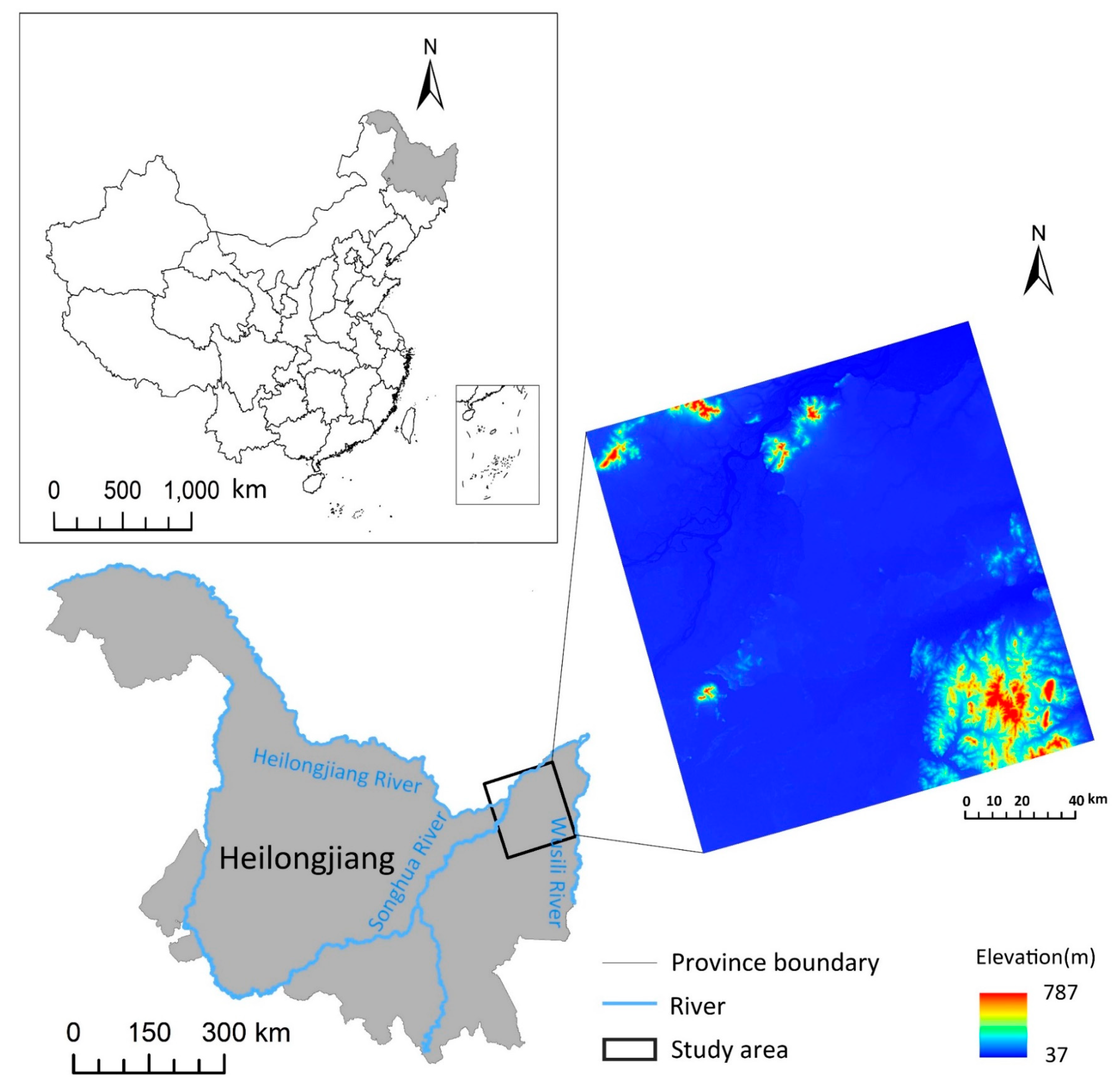
The Sanjiang Plain, located in Northeastern China, is an alluvial plain formed by the confluence of Heilongjiang River, Wusuli River and Songhua River. It has a humid and semi-humid continental climate region and belongs to the temperate zone. Annual precipitation is about 500–650 mm and mainly falls between June to October. The agriculture land is primarily cultivated with paddy rice, maize, bean and some vegetables. Rice seeds are usually sown in mid-April, and rice seedling plants are transplanted to paddy rice fields between mid-May and early June. Flooding is usually carried out about two weeks before rice transplanting, and it is a key practice in rice agriculture. Rice plants are mature in late September and harvested in early October. Corn and soybean are planted from mid-to-late May and are mature at almost the same time as rice. Other vegetation such as evergreen forests and wetlands usually have longer growing seasons than rice, corn and soybean. In recent years, the paddy rice planting area in the Sanjiang Plain has been increasing, resulting in a decrease in wetland area and a sharp increase in farmland [33]. It was reported that the rice production in Sanjiang Plain has reached 13% of the total amount of rice production in China [34]. We chose a part of the Sanjiang Plain as a pilot study area (Landsat Path/Row: 114/27). The study area is located between 46°05′33.70″–48°02′26.12″N, 132°00′39.13″–133°08′42.03″E, and has large areas of croplands, water bodies, buildings, forests, marshes (wetlands) and other land cover types. The paddy rice fields in the study are distributed in a scattered manner (Figure 1).
2.2. Data and Pre-Processing
2.2.1. Landsat Data and Pre-Processing
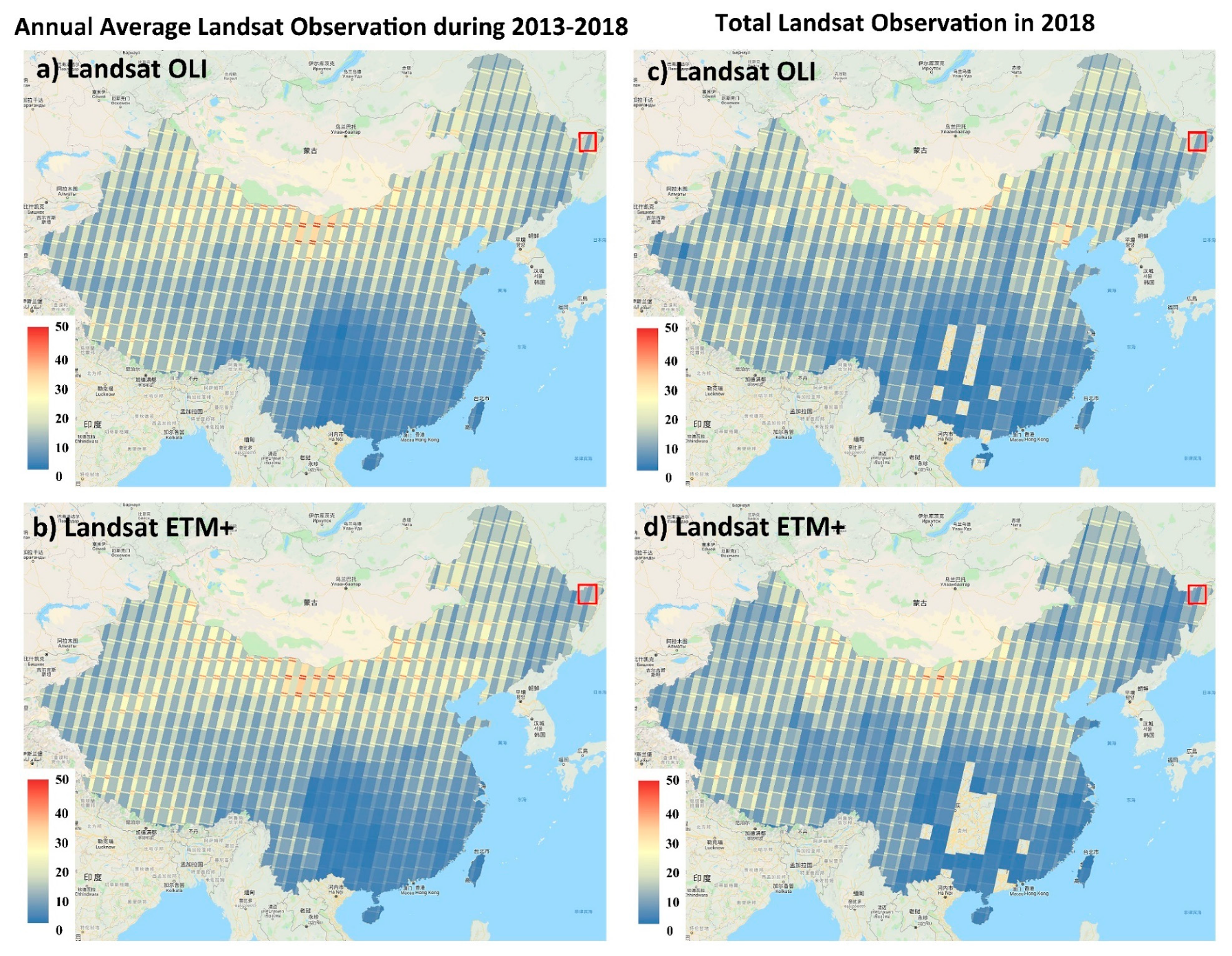
In order to examine the availability of the Landsat data, the Google Earth Engine platform (GEE, https://earthengine.google.org) was used to count the number of all available Landsat images (Landsat ETM+, Landsat OLI) over China [35]. Figure 2 shows the annual average numbers of Landsat images during 2013–2018 (Figure 2a,c) and the total number of 2018 (Figure 2c,d) with a cloud cover of less than 10% respectively. As illustrated, there are few Landsat images available especially in the southern and northeastern regions, while those regions are the main rice production areas in China (most less than 10 images). Due to the long revisit period (16 days) and the impacts from clouds and rain, the actual available data is too few to meet the requirement of the phenology-based algorithm.
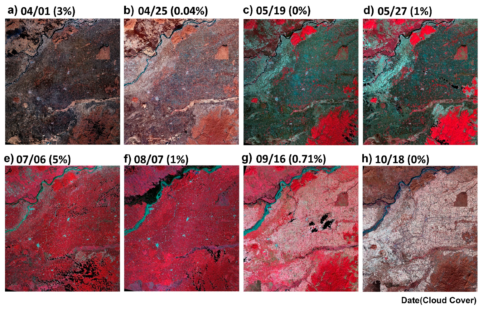
In the study, all available Landsat 7 (ETM+) and Landsat 8 (OLI) surface reflectance data (path/row: 114/27) of the study area with cloud cover less than 10% in 2018 were obtained, except for the images with large areas of snow cover in winter. The total number of qualified images is seven. All Landsat images used in the study were standard terrain-corrected (L1T), radiation-corrected, and geometric-corrected images, and had been atmospherically corrected to surface reflectance using LEDAPS (Landsat ETM+) [36] and Land Surface Reflectance Code (LaSRC) (Landsat OLI) [37]. All possible bad observations affected by clouds, cirrus clouds or ice/snow with confidence levels of 67–100% were excluded from Landsat images using the quality assessment band (QA). The SLC-off strips in the Landsat ETM + images were classified as “no value” [38]. Then, we cropped all images to the geographic extent of the study area. Finally, Landsat images after preprocessing were used for the STARFM and phenology-based classification (Figure 3).
2.2.2. MODIS Data and Pre-Processing
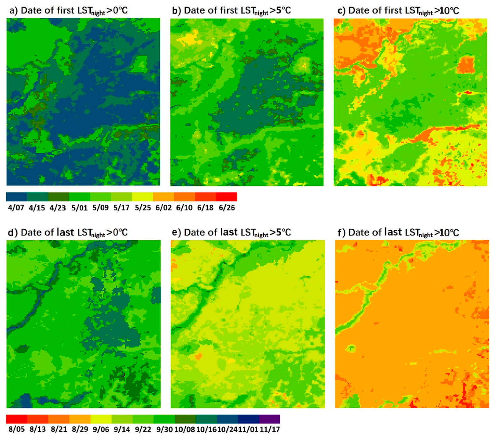
The MOD09A1 Version 6 is an eight-day composite 500-m MODIS surface reflectance product. The MYD11A2 Version 6 data can provide eight-day average values of nighttime clear-sky LSTs. All the MODIS products covering the study area were downloaded from the United States Geological Survey (USGS) and re-projected to the UTM-WGS84 Zone 53N projection. Then, all images were cropped to keep the same size with Landsat images exactly. For MOD09A1 images, pixels contaminated by clouds were masked based on the MODIS quality flags. The MYD11A2 products were used to define phenology timing and crop calendar. The starting dates of temperatures above 0, 5 and 10 °C were calculated and then the resultant maps of the starting date of stable temperatures above 0, 5 and 10 °C were generated (Figure 4). Finally, all MOD09A1 images and the resultant maps were resampled to a spatial resolution of 30 m using the nearest neighbor interpolation to be spatially consistent with the used Landsat images.
2.3. Additional Datasets
Ancillary datasets including elevation data and forest map were used to improve paddy rice classification. The elevation data was Shuttle Radar Topography Mission (SRTM) Digital Elevation Data Version 4 from the CGIAR-CSI SRTM 90 m Database (http://srtm.csi.cgiar.org) and the forest map was obtained from ALOS/PALSAR-based fine resolution (25-m) global forest map (https://www.eorc.jaxa.jp/ALOS/en/palsar_fnf/data/index.htm) [39]. In addition, the phenology calendar of major plants in the study area acquired from the Ministry of Agriculture and Rural Affairs of the People’s Republic of China (http://www.moa.gov.cn) was used to validate the accuracy of the temperature-defined plant growing season and flooding and transplanting period of paddy rice.
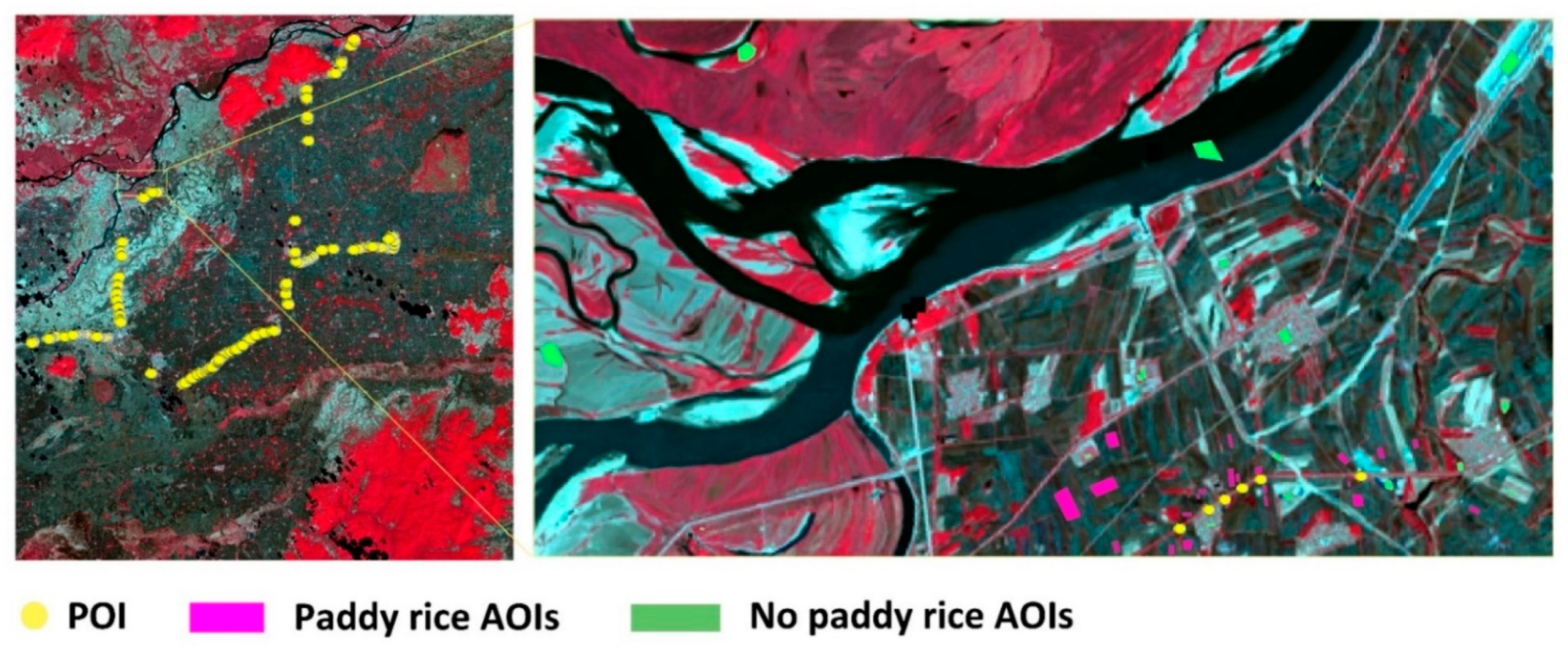
Reference samples were visually interpreted from (1) high resolution image collections from Google Earth, and (2) the 311 geo-referenced field photos mostly collected in May 2017 from the Global Geo-Referenced Field Photo Library (http://www.eomf.ou.edu/photos/). The geo-referenced field photos were converted into points of interest (POIs) in kmz format for displaying in Google Earth. In those photos, rice fields were usually farmland covered by water. A total of 711 vector polygons (Areas of Interest, AOIs) were drawn around the acquired POIs by referring to both the field photos and the Google’s historical high-resolution images, including paddy rice (347 AOIs, 9997 pixels) and non-paddy rice (332 AOIs, 9908 pixels) (Figure 5). The area of paddy rice AOIs (900 ha) is close to non-paddy rice AOIs (892 ha). Those AOIs contained only one kind of land cover and their boundaries kept a distance of over 30 m away from the boundaries of other land cover types. The detailed non-paddy rice AOIs generation method was as follows: the non-paddy rice land cover types were divided into five major types: upland crop, forest, wetland/swamp, water body, and built-up land, according to the auxiliary data in Section 2.3 and the paddy rice map from Qin et al. (2015) [3]. Random points in the study area were generated in each stratum by referring to the high-resolution images from Google Earth and field photos, and then non-rice AOIs were generated around the random points with the same method as paddy rice AOIs. The Google historical images used in the AOI drawing process were mainly in 2016–2018.
3. Method
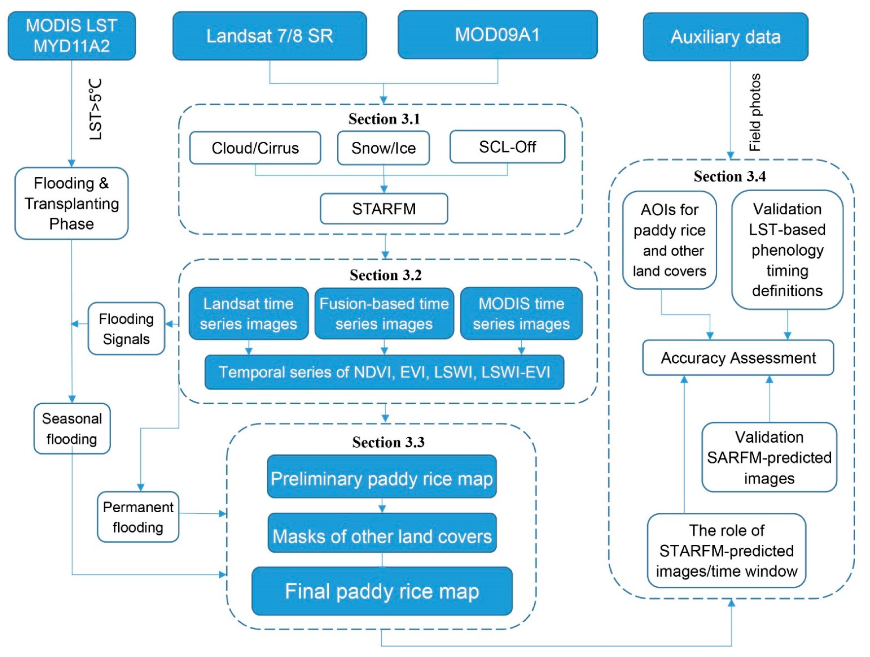
The fusion- and phenology-based paddy rice mapping methodology (Figure 6) mainly involved the following steps: (1) STARFM prediction by using images after pre-processing (Landsat ETM+/OLI, MODIS); (2) Calculation of time series VIs, namely EVI, NDVI, and LSWI; (3) Mapping paddy rice fields using the phenology-based algorithm; and (4) Accuracy Assessment.
3.1. STARFM Prediction
STARFM is the most widely used spatiotemporal fusion model, which has stable and reliable performance in predicting fine resolution images [40,41]. In the study, STARFM was used to fuse Landsat and MODIS surface reflectance data to generate Landsat-like images. The algorithm was proposed based on two assumptions: (1) if MODIS and Landsat surface reflectances are equal on date , then they should be equal at date ; (2) if no change happens in the MODIS surface reflectance, then no change should be predicted at the Landsat spatial resolution [22]. STARFM takes into account the spectral and spatial similarities between pixels, using one or two base pairs of Landsat and MODIS images at date and one MODIS image for the prediction date to predict a synthetic Landsat-like image with a 30 m spatial resolution at the prediction date [22]. In order to minimize the effect of pixel outliers, the algorithm uses a moving window from fine-resolution images (Landsat) to search for similar pixels by using spatial, temporal and spectral information. Then, the surface reflectance for the central pixels of the window at date is computed with a weighting function by introducing additional information of similar pixels as follows:
where is the searching window size, is the central pixel of the moving window, and is the weight to decide the contribution of the similar pixels to the estimated reflectance of the central pixel. is the predicted surface reflectance of pixel with the fine resolution at date . , are the surface reflectances of MODIS pixel at date and , respectively. is the surface reflectance of Landsat pixel at date . More detailed descriptions of the algorithm can be found in Gao et al., 2006 [22].
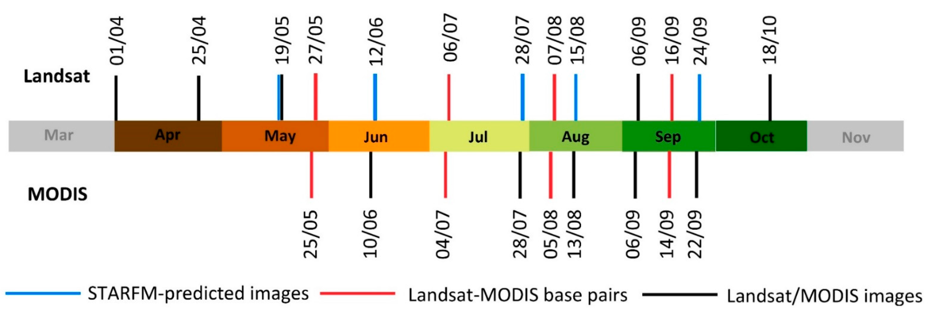
In the study, the MODIS images used in STARFM were selected based on the date of available Landsat images to minimize the time interval between the base pair. In addition, the time interval between the acquisition date () and the prediction date () was also taken into consideration for more precise fine images. In order to capture spectral characteristics during key phenology phases (e.g., rice flooding and transplanting period) and remove noises from other vegetation and crops, we tried to make Landsat and Landsat-like images distributed evenly during the growing season. Finally, the STARFM-predicted images combined with the real Landsat images were assembled into a time series dataset (hereafter referred to as ‘fused time series data’) ready for phenology-based paddy rice mapping. The Landsat and MODIS images used in STARFM and the Landsat and STARFM-predicted images used in the phenology-based algorithm are shown in Figure 7.
3.2. Fused Time Series NDVI and EVI and LSWI Data
In the phenology-based algorithm, the paddy rice fields can be identified by its unique physical characteristics. The characteristics can be detected by using the relationship between the time-series LSWI, NDVI and EVI [13,16,42]. The three indices are widely used in the study of vegetation canopy, biomass and phenology. Therefore, for each image in the fused time series data, we calculated the NDVI, EVI, and LSWI using the surface reflectance values of the blue band (), red band (), NIR band () and SWIR band (). The functions are as follows:
In addition, we calculated the difference between LSWI and EVI () and the difference LSWI and NDVI () for each image in the fused time series data. Finally, for comparison purposes, we also obtained another two sets of VIs (EVI, NDVI, and LSWI) data calculated from the Landsat only dataset and the MODIS only dataset, respectively.
3.3. Identification of Paddy Rice Fields
3.3.1. Algorithms to Identify Inundation/Flooding Signals
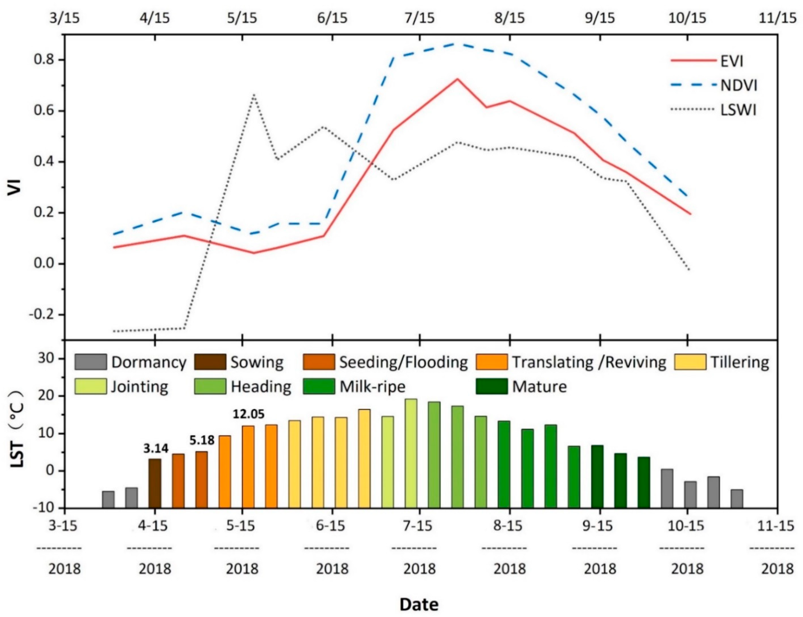
In the study, only paddy rice, natural wetlands, and some vegetation (e.g., grass, trees, and shrubs growing on the edge of water bodies) have flooding/inundation events/signals. Previous works have proved that LSWI-NDVI 0 or LSWI-EVI 0 coincide with flooding events [13,16,42]. Generally, the pixels identified as flooded are a mixture of water and plants during the whole year [9]. For paddy rice, this phenomenon can be found in Figure 8. Paddy rice is the only crop that needs to be transplanted into a mixed environment of water and soil. Before transplanting, paddy rice fields are covered with water. After transplanting, as rice plants grow in flooded fields, rice fields are a mixture of rice plants, soil and water (open-canopy stage). Then, rice plants continue to grow until plants canopy completely covers the fields. In the open-canopy stage, the indices of paddy rice fields have unique temporal characteristics: the LSWI values of paddy fields are higher than their NDVI and EVI values. This phenomenon is called flooding events/signals (Figure 8).
Paddy rice transplanting date varies in different regions. Identification of the growing season and the flooding/transplanting period of paddy rice could help us select images at appropriate times for better distinguishing paddy rice from other vegetation types [10,14,31], and improve the efficiency of paddy rice field detection. Crops need certain accumulated temperatures to complete their life cycle, so it is more reliable to use nighttime LST as a physical indicator for biophysical limitation [7]. Hence, the nighttime MODIS LST data was used to determine the growing season and the paddy rice flooding/transplanting of the study area. First, the first and last dates of nighttime LST larger than 0 C were extracted as the start and end dates of the plant growing season of the study area (Figure 4a,d). Second, according to previous studies, the start date of nighttime LST above 5 °C or 10 C was determined as the likely start date of flooding and transplanting (SOF) [10,31]. Then, by comparing the temporal profiles of VIs and nighttime LST (Figure 8, the flooding signals of paddy rice fields mainly occur before the date that LSWI and EVI curves cross), the start date of nighttime LST over 5 °C was close to the SOF in the study (Figure 4b). The flooding signals of paddy rice can last for about two months after transplanting until rice canopy almost covers the entire fields [13], so the length of the flooding/transplanting phase was SOF+60. The phenology stages recorded by the phenology calendar matched well with the temperature-defined plant growing season and the temperature-defined flooding and transplanting period of paddy rice (Figure 8).
Considering that NDVI is limited under a closed canopy and soil background [43], and EVI is more sensitive to NIR and more robust to biomass variation [44], we marked the pixels with flooding signals by using rule LSWI-EVI 0 for each image during the flooding and transplanting period. Then we assumed pixels with flooding signals to be “potential or likely” paddy rice pixels and got a preliminary paddy rice map.
3.3.2. Implementation of Phenology-Based Paddy Rice Mapping Algorithm
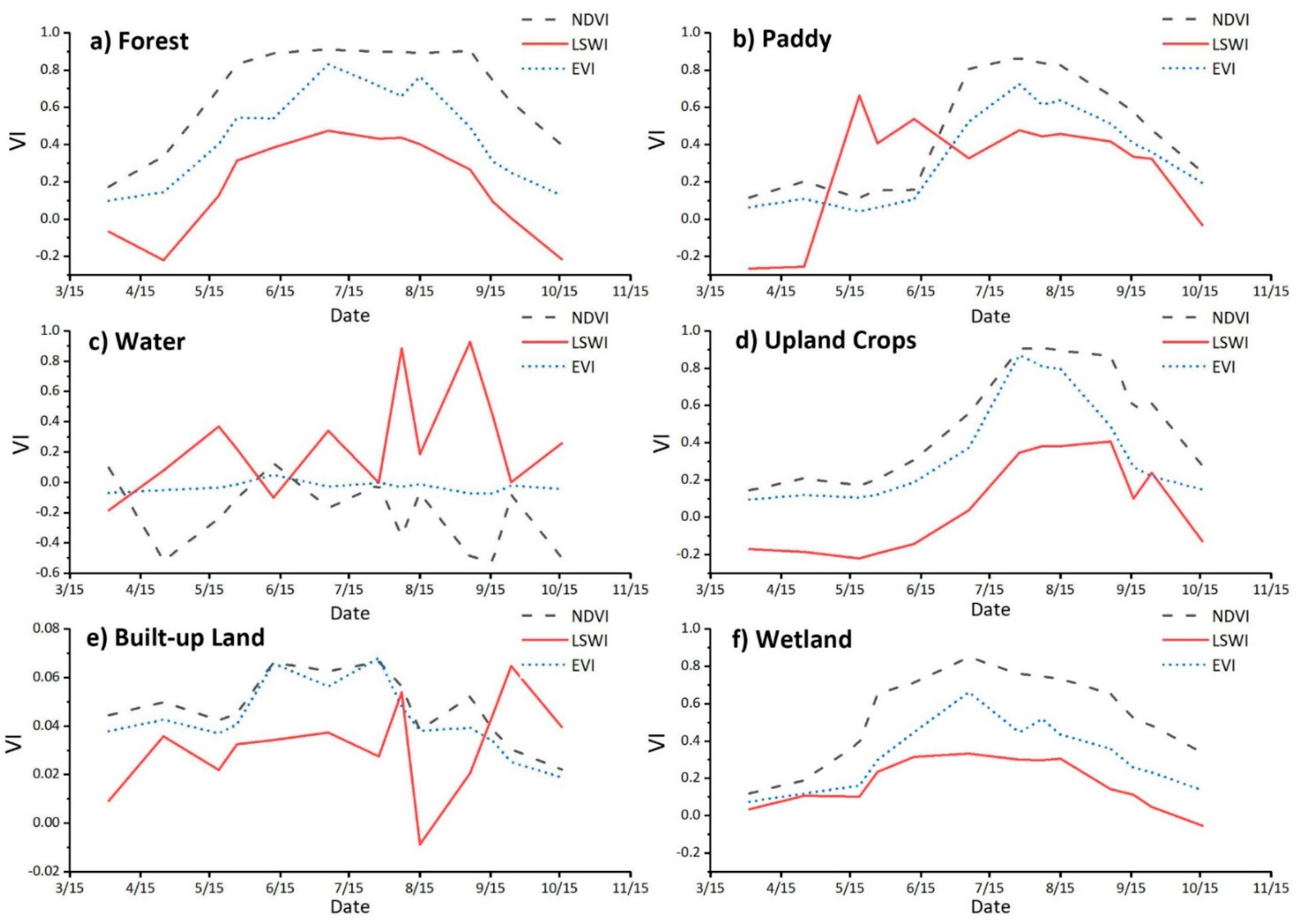
Influenced by factors such as atmospheric conditions and other land cover types that have some similar physical characteristics to paddy rice, the preliminary paddy rice map was inevitably polluted by noises. Therefore, according to the phenology characteristics and the temporal profiles of VIs of other land cover types in the study area (Figure 9) [3,9,14,31], masks were established to remove these noises as follows:
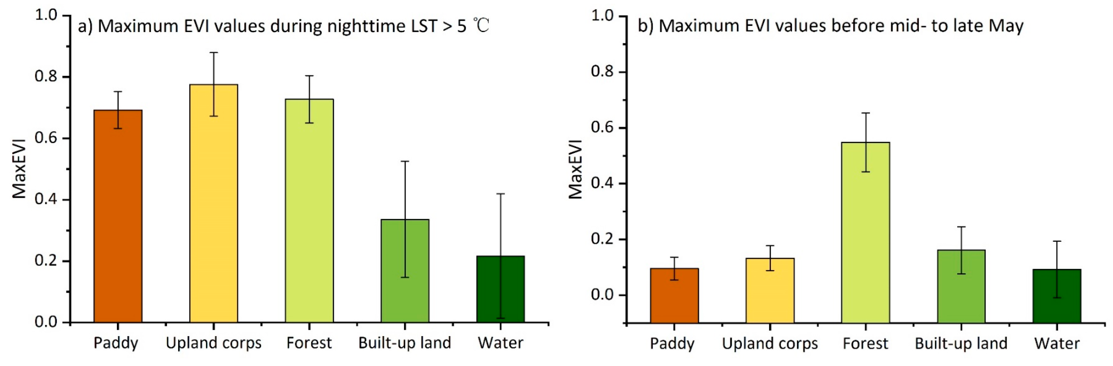
- Natural vegetation. Forests, grasslands and shrubs grow earlier and are greener than paddy rice, so the EVI values of natural vegetation are higher than the EVI values of paddy field before the rice plants begin to grow. We identified the pixels with maximum EVI value ≥ 0.30 before the mid-flooding/transplanting period (corresponding to the images before May 29 in the study) as natural vegetation and generated a preliminary mask of natural vegetation. Then we combined the preliminary mask with the ALOS/PALSAR-based fine resolution (25 m) forest map (2017) to get a final natural vegetation mask.
- Sloping land. Rice plants grow in water and therefore cannot be planted in sloping land. The sloping land mask was generated based on the rule of slope ≥ 3° to exclude the areas with low probabilities of growing paddy rice by using the SRTM DEM data.
- Sparse vegetation. There are some low-vegetated lands in the field roads, built-up land, water edge and other areas. Those low-vegetated lands have very low greenness within the entire growing season (Figure 9 and Figure 11). Thus, pixels with the maximum EVI value ≤ 0.60 within the plant growing season (nighttime LST > 0 °C) were labeled as sparse vegetation. In addition, the preliminary paddy rice map had obvious strips. That was mainly because the EVI values of paddy rice pixels reached their maximum from July to August, while the images in July all contained SLC-off gaps from Landsat ETM+. Therefore, the maximum EVI values of paddy rice pixels in the strip region were mostly replaced by the paddy rice EVI values from images in September, and those paddy rice pixels were misclassified into sparse vegetation. Referring to the dates of the Landsat ETM+ images in the fused time series data, pixels in the strip region with the maximum EVI value ≤ 0.55 within the plant growing season (nighttime LST > 0 °C) were classified as sparse vegetation.
- Open canopies in permanent flooding areas, such as vegetation (grass, trees, shrubs) growing on the edge of water bodies. Pixels in the open canopies are a mixture of natural vegetation and water and have flooding signals. Therefore, it is necessary to distinguish open canopies in permanent flooded areas from open canopies in seasonally flooded areas. Unlike seasonal flooding areas such as rice fields, permanent flooded areas usually have flooding signals throughout the entire growing season. Therefore, if a pixel had the flooding signal for all images within the entire growing season, then it was marked as a permanent flooded canopy.
- Natural wetlands. There are natural wetlands in the Sanjiang Plain due to long-term waterlogging. When the temperature rises above 0 °C, natural wetlands start to flood due to snowmelt. Therefore, wetland vegetation has grown a few weeks before the flooding signals appear in paddy rice fields. The difference in EVI values between the wetland vegetation and paddy rice reaches to the maximum around the middle of June (Figure 9 and Figure 10). Therefore, if a pixel with flooding signals had maximum EVI value ≥ 0.30 between LST > 0 °C and mid-June after excluding the masks described above, then it was classified as natural wetlands.
Finally, all of the pixels in the above mask were excluded from the preliminary paddy rice map and obtain a final paddy rice maps (hereafter referred to as ‘the fusion-based paddy rice map’).
3.4. Evaluation of Fusion-and Phenology-Based Paddy Rice Map Strategy
3.4.1. Evaluation of STARFM Prediction
We evaluated the accuracy of STARFM predictions by comparing the STARFM-predicted images with the real Landsat images. The images used as input data and validation data are shown in Table 1. For example, the Landsat image on 27 May, the MODIS image on 17–25 May were used to predict the Landsat-like image on 19 May, and then the Landsat-like image was compared with the original Landsat image on 19 May for evaluation.
We selected three groups of data to evaluate the accuracy of STARFM-predicted images in different situations, including (1) using one fine resolution image to predict the Landsat-like image of the latter date (Prediction Tests 1 and 3), and (2) using one fine resolution image to predict the Landsat-like image of the previous date (Prediction Test 2). In addition, the time interval between date and date was also taken into consideration: the time interval of the Prediction Test 3 was close to one month, which was much longer than Prediction Test 1 and Prediction Test 2 (eight days).
We employed the root mean square error (RMSE), correlation coefficient (r) and absolute average error (AAD) of predicted reflectance compared with real reflectance (including blue, green, red, NIR, SWIR1 and SWIR2 bands) to quantitatively assess the accuracy. AAD can reflect the difference between fusion images and real images. The closer the AAD is to zero, the better the prediction is. r can well detect the consistency between fusion images and real images. The closer the r is to one, the more similar the fusion images are to the real images. RMSE can well measure the deviation of fusion images from real images. The smaller the RMSE, the better the prediction. The functions are shown in Formulas (5)–(7).
where is the number of pixels involved in the calculation, is the value of each pixel in fusion images, is the value of each pixel in the corresponding real image, , are the mean values of and , respectively. Moreover, the RMSE, r, AAD between fused NDVI/LSWI/EVI values and Landsat NDVI/LSEI/EVI values were calculated to assess the performance of the key VIs used in the study.
3.4.2. Comparison with Other Classification Results
For comparison purposes, we used the same phenology-based strategies to generate two additional maps from Landsat images only and from MODIS time series images, respectively. We also compared the fusion-and phenology-based strategy with the random forest (RF) classification method. RF is a well-known, widely used learning-based algorithm. In this study, RF was chosen for its stability since it is not sensitive to noise. Then RF was employed based on the same set of features, i.e., time series NDVI, EVI, LSWI and LSWI-EVI from each of the 13 Landsat and Landsat-like images. For the RF classifier, we generated ROIs for all land cover types (i.e., paddy rice, upland crop, forest, wetland/swamp, water body, and built-up land) in the same way described in Section 2.3 to support classification (16,371 pixels). Two parameters were defined as follows: the number of the trees was set to 200, and the number of the random variable to split each node of the individual tree was set to eight. First, 200 bootstrap samples were drawn from the 2/3 of the training data set. The remaining 1/3 of the training data called out-of-bag data was used for evaluating the performance of RF. Then, the decision trees were constructed based on randomly selected features of the bootstrapped sample. Finally, the class label of each pixel was determined by the majority voting of the decision trees. The classification result was divided into two categories as well: paddy rice and others. At the same time, the feature importance (namely variable importance in RF) was obtained, which allowed us to analyze the importance of each image and different time windows. The feature importance was estimated by the degradation of model prediction, caused by the random permutation [45]. Then we used the same set of reference samples as in the accuracy assessment of the phenology-based paddy rice map to evaluate the four classification results by comparing the map class and reference class at the reference sample locations. The number of samples for training the models in RF was close to the number of samples for accuracy assessment.
4. Result
4.1. Accuracy of the STARFM Predictions
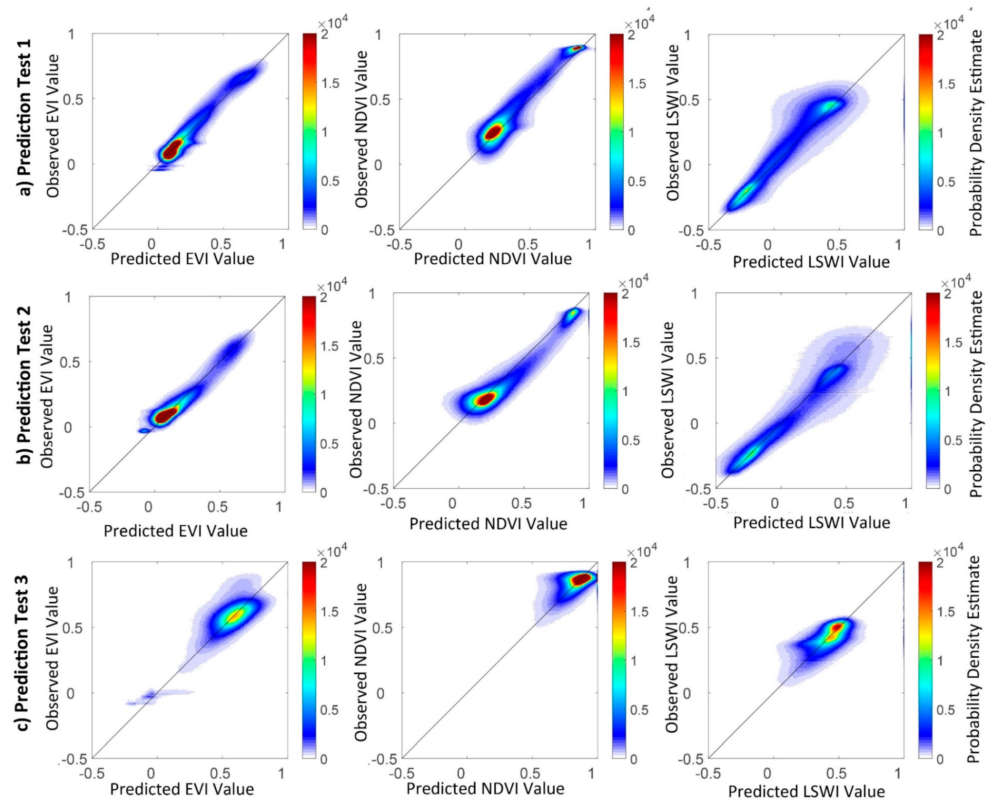
Scatter density plots in Figure 11 show the relationships of the VIs between the predicted and the actual values of Prediction Test 1/2/3. All the data in the scatter density plots fall close to the 1:1 line. Therefore, all the results show that the STARFM algorithm can predict the fine resolution images with high accuracy and reliably express the spectral information of the Landsat image in the corresponding period.
Table 2 and Table 3 list the results of AAD, RMSE and r calculations on the six bands and VIs between the predicted images and the real images. For reflectance (six bands), the RMSE values vary from 0.01 to 0.08, r values range from 0.66 to 0.93, and AAD values vary from 0.01 to 0.05; for VIs, the RMSE values vary from 0.05 to 0.27, r values range from 0.71 to 0.96, and AAD values vary from 0.03 to 0.16. Generally, the comparison between real Landsat and STARFM-predicted images show high correlations and small biases, both for reflectance (six bands) and VIs. The fusion image of Prediction Test 3 shows greater errors and lower correlations than the fusion images of Prediction Test 1 and 2. The AAD and RMSE values of Prediction Test 3 (ranges from 0.01 to 0.05, and 0.01 to 0.08, respectively) were generally larger than Prediction Test 1 (ranges from 0.01 to 0.03, and 0.02 to 0.04, respectively) and Prediction Test 2 (ranges from 0.02 to 0.04, and 0.01 to 0.05, respectively). The r values of prediction Test 3 (ranges from 0.65 to 0.73) were smaller than Prediction Test 1 (ranges from 0.79 to 0.93) and Prediction Test 2 (ranges from 0.79 to 0.93). One potential explanation for the relatively low accuracy of Prediction Test 3 may be due to that its time interval between base date and prediction date was larger than the other two. In Prediction Test 3, the paddy rice has undergone more rapid growth around August, which further makes the difference between the image on the base date and the image on the prediction date larger and brings more errors to the fused image. There is a small difference between the image predicted by the real image on the previous date and the image acquired by the real image on the later date (Prediction Test 1 and 2). Therefore, when using real fine images to predict images, the images before and after the prediction date both can be taken into consideration. However, the time interval between the acquisition date and the prediction date needs to be taken into consideration. In the study, all the situations above have been taken into consideration for more precise, predicted images.
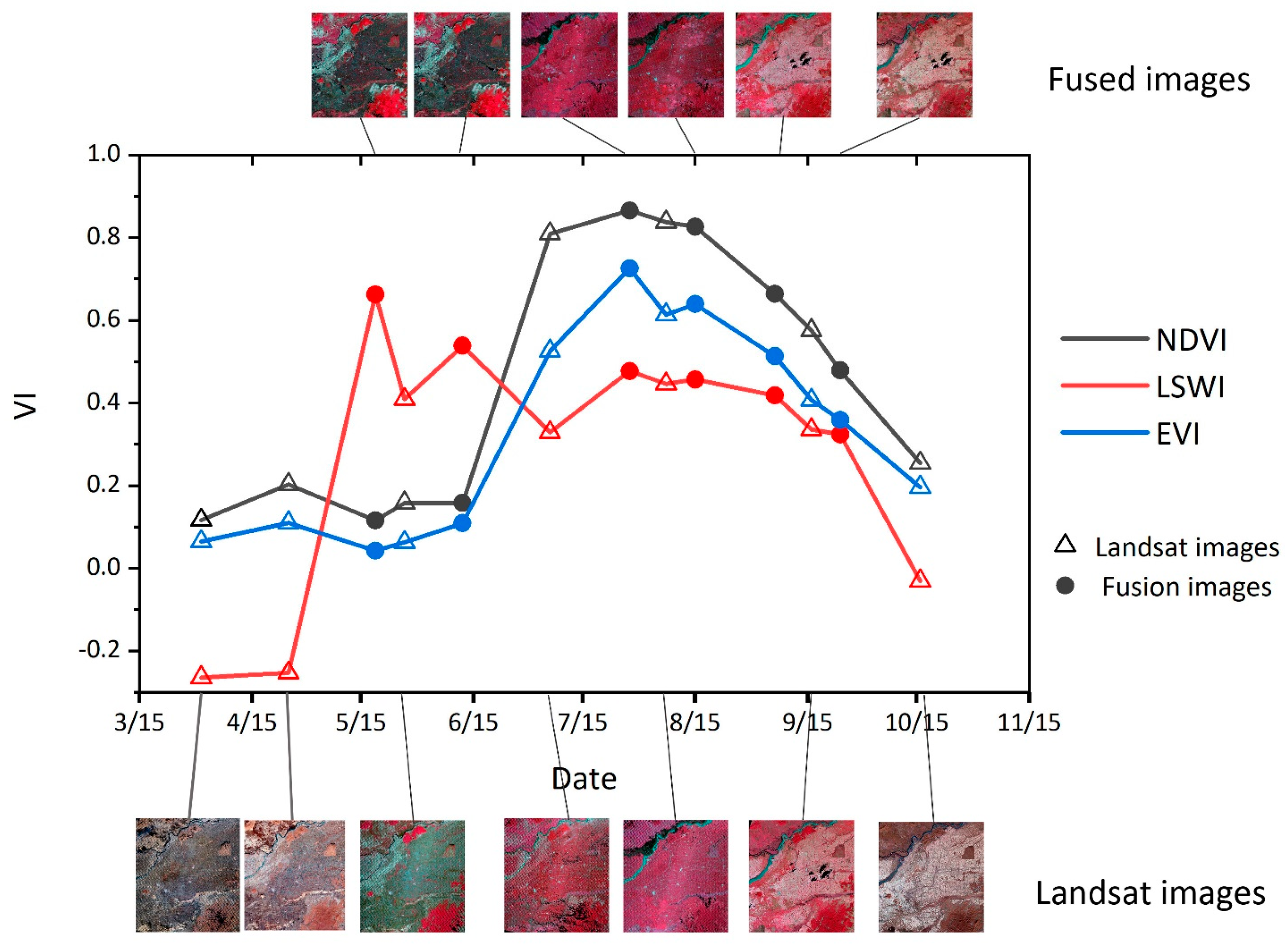
Figure 12 shows an example of temporal profiles of paddy rice vegetation indices (NDVI, EVI, and LSWI) extracted from fused time series data. We can see clearly the growing cycle of paddy rice, with the growing season peaks around July 28, the flooding and transplanting period starts around May 1 and ends around July 1. It is worth noting that if we only use Landsat data, we will get a much narrower time window corresponding to the flooding and transplanting period and will have few available scenes during the peak growing season.
4.2. Comparisons with Non-Fusion-Based and RF Classification Results
In order to verify the availability of the new strategy in paddy rice field mapping, the MODIS and the Landsat time series imagery were also used to map paddy rice by using the same classification strategies described in Section 3, respectively (hereafter referred to as ‘the Landsat-based paddy rice map’, ‘the MODIS-based paddy rice map’). In addition, the RF classification method was used to map paddy rice based on the same fused time series data (hereafter referred to as ‘the RF-based paddy rice map’). The results of the above four classifications are shown in Figure 13. Most of the paddy rice fields were distributed in flat areas near rivers, which was consistent with the real situation.
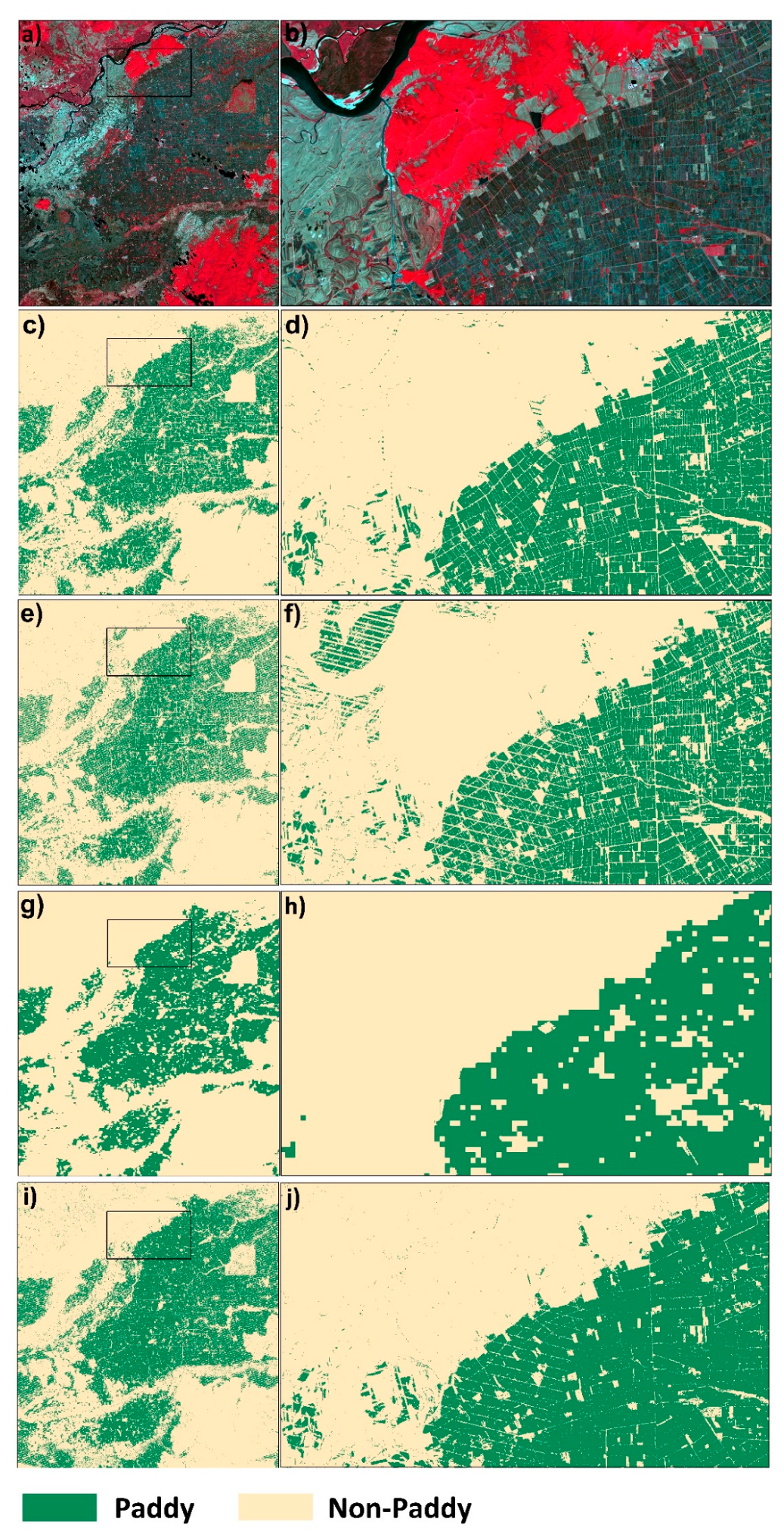
All maps maintained good spatial consistency. Compared with the Landsat-based map (Figure 13e,f), the map based on the fused time series data (Figure 13c,d) can better distinguish paddy rice from wetland/swamp vegetation, and had higher classification accuracy for paddy rice fields, especially the paddy rice fields near rivers, wetlands, and marshes. In addition, the fusion-based classification can effectively remove the SLC-off gap effects by using the phenology-based algorithm. However, the Landsat imagery can hardly exactly extract phenology information such as the maximum EVI/NDVI value due to data limitation (Figure 12). Thus, there were some commission errors, omissions errors and obvious SLC-off gap effects in the Landsat-based map. Compared with the MODIS-based map (Figure 13g,h), the fusion-based map contained more spatial details. For example, it can clearly show some patchy and fragmented paddy rice fields and the roads between paddy rice fields, which were omitted on the MODIS-based map. Compared with the RF-based map (Figure 13i,j), the fusion-based map also contained more spatial details for it can clearly show the roads between fields. The paddy rice fields estimated from the Landsat-based map and the MODIS-based map accounted for about 29.38% (6.48 × 10⁴ ha), 32.11% (7.08 × 10⁴ ha) of the study respectively, which were smaller than that estimated from the fusion-based map (33.46%, 7.38 × 10⁴ ha).
Confusion matrices in Table 4 show that the overall accuracy and Kappa coefficient of the fusion-based paddy rice map were 98.19% and 0.96 respectively, which were larger than the MODIS-based paddy rice map (89.23%, 0.78) and the Landsat-based paddy rice map (92.12%, 0.84). The difference between the fusion-based map and Landsat-based map mainly in the classification of sparse vegetation in the areas of strips and wetlands. Greater commission and omission errors were found in the MODIS-based map. Therefore, the combination of fusion images, Landsat ETM + and OLI can make the phenology-based algorithm more powerful in mapping paddy rice fields and improve classification accuracy. Furthermore, for comparison purposes, the overall accuracy and Kappa coefficient of the RF-based paddy rice map were calculated in the same way, and were 93.53%, 0.87 respectively. This further indicates that our classification strategy used in this paper can obtain higher classification accuracy.
4.3. Evaluation of the Feature Importance
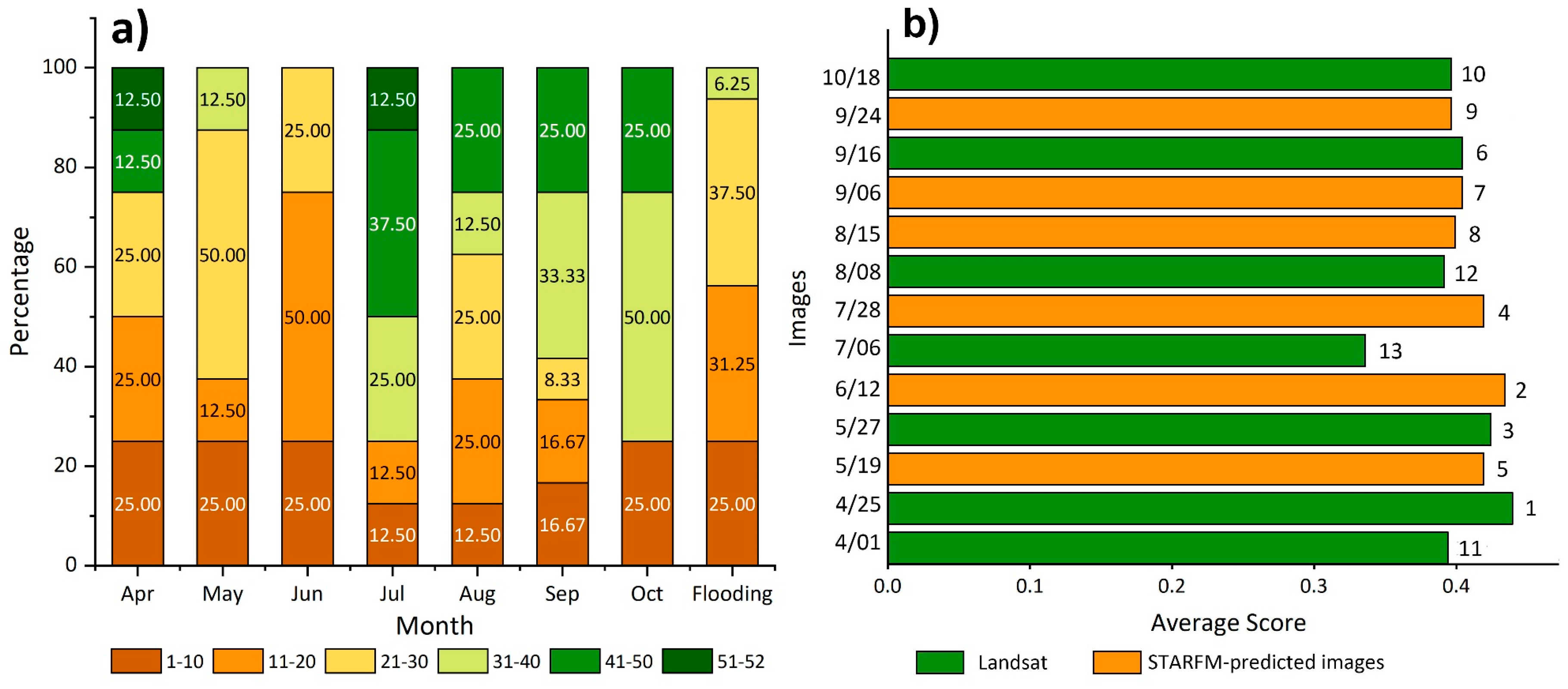
All 52 features were sort into six groups by variable importance in descending order. For all features in one time window (e.g., each month), the number of features in each group was counted and then its percentage in all features of the time window was calculated (hereafter referred to as ‘the percentages of each group’). The importance of each month and the entire transplanting and flooding period was evaluated by the percentages of each group (Figure 14a): the higher the percentage of the crucial groups in the time window, the higher the importance of the time window. The importance of each image was presented by the average score of its feature importance (Figure 14b). On the one hand, the result shows that April, May and June contributed more than other months to the classification. Especially, the images within the transplanting and flooding period played an important role in the classification, which shows the importance of the images in the key phenology period for paddy rice identification. From Figure 8 and Figure 12, the flooding and transplanting period starts around May 1 and ends around July 1. This may explain why April, May and June were deemed as the important time window in mapping paddy rice and prove the importance of the images from the transplanting and flooding period. On the other hand, the result indicates that almost all the images within the planting growing season have provided valuable information for distinguishing different land cover types. Fused images were mostly ranked with higher importance. The potential explanation for the relatively high importance of fused images may be due to it has filled the gap of data in the flooding and transplanting period and peak growing season (Figure 12) that play an important role in distinguishing different land cover types. This further proved the necessity and the importance of those fusion images used in the classification.
5. Discussion
5.1. Advantages of Fusion-and Phenology-Based Paddy Rice Mapping Strategy
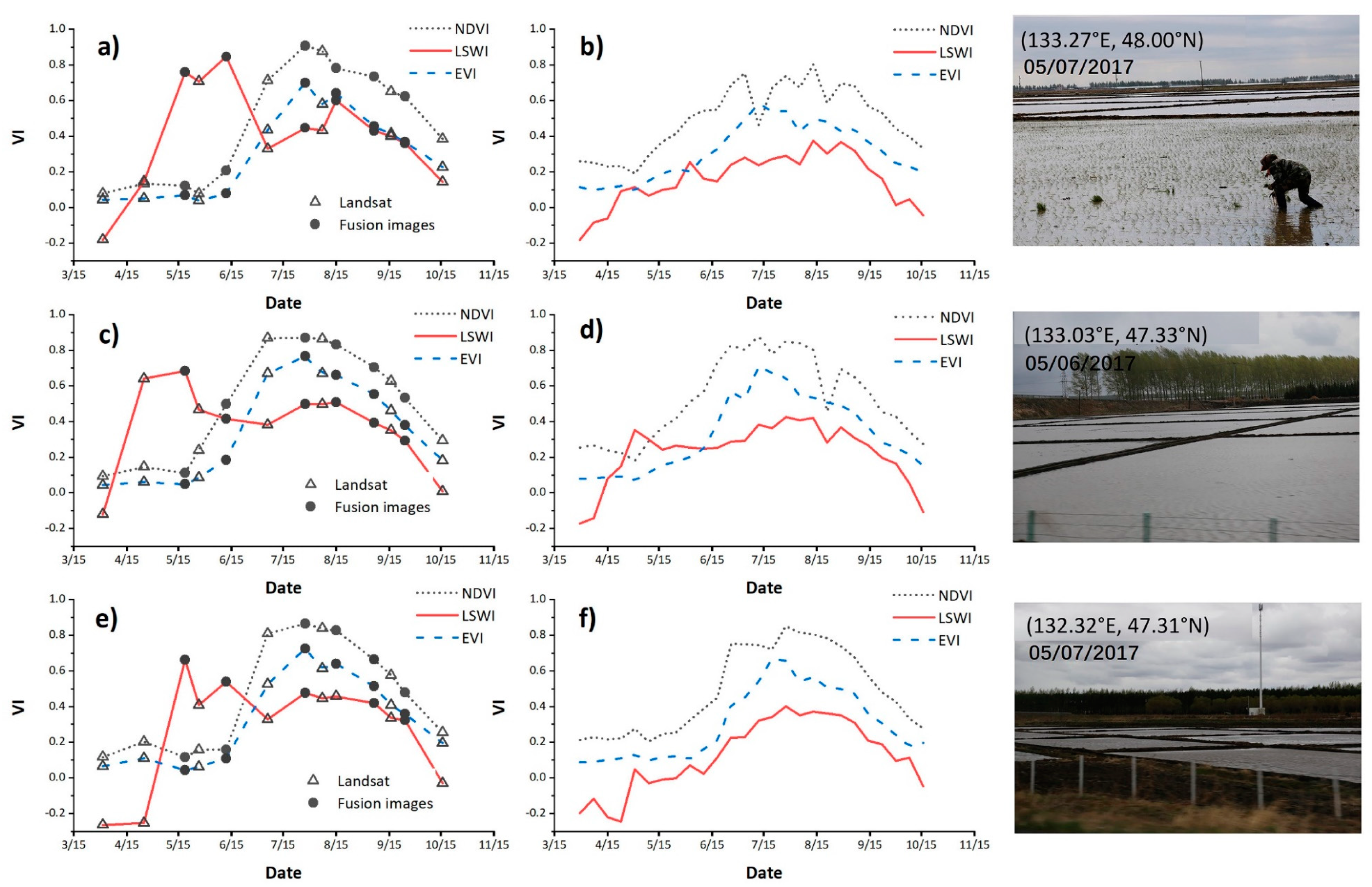
High-quality observations during paddy rice growth period are essential for paddy rice field mapping. There are persistent and heavy cloud coverages in most paddy rice planting regions, which brings uncertainties and noises to paddy rice classification due to those unfavorable observing conditions. Therefore, the ultimate goal of the study is to provide a pathway leading to an operational strategy for paddy rice mapping by alleviating or overcoming the data limitation to some degree. To achieve the goal, we presented a new strategy by integrating the STARFM spatiotemporal fusion algorithm and phenology-based algorithm. Our results show that the strategy performs better than the conventional phenology-based algorithm using MODIS data alone or using Landsat data alone. The paddy rice map shows more spatial details and lower errors than the Landsat-based and MODIS-based maps. This is mainly because that the fusion data helps recover the temporal profiles of VIs, which play an essential role in identifying unique phenological characteristics of paddy rice. The comparisons with the existing MODIS-map by Zhang et al., 2015 [17] and the existing Landsat-map by Dong et al., 2015 [14] also confirm that our map has more spatial details and fewer omission errors especially in SLC-off strip areas and regions with patchy and fragmented fields. Figure 15 compares the temporal profiles of VIs extracted from time series Landsat and Landsat-like data with those extracted from MODIS data at three sites (all the three sites were selected according to field photos). It can be seen that the EVI/NDVI values from the fused time series data show similar trends with those from MODIS data. Generally, the VIs based on the red-edge and NIR bands have strong correlations with LAI and are sensitive to the dynamics of the canopy and surface water content [17,46]. Therefore, the NDVI, EVI, LSWI should ideally capture the unique physical features of paddy rice during the flooding and transplanting phases. However, the MODIS LSWI time series failed to depict the flooding signals during the paddy rice transplanting and flooding period because of its low spatial resolution and mixed pixels. During the flooding and transplanting period, the LSWI values from the MODIS time series (the maximum LSWI value was lower than 0.40) were much smaller than those from the fused time series data (the maximum LSWI value was over 0.60). Using Landsat data alone cannot capture greening and maturing signals of rice plants. From Figure 15a,d,g, the increasing trend of NDVI/EVI values from May to July and decreasing trend from July to November were well reconstructed by the fused time series data. Therefore, the fusion images are desirable to capture phenological information and for paddy rice classification.
Previous researches [23,32] reported that using all of the time-series Landsat and fused Landsat-like data for land cover classification may be not a judicious choice. However, in our study, we found that the utilization of time-series Landsat imagery is necessary. In their studies, SVM was used for classification. Redundant information in the spectral time series might cause overfitting and lower generalization power of SVM, thus leading to larger errors. Different from the training-based classification, the phenology-based algorithm used in our strategy relies on a clear phenological pattern to select the threshold suitable for paddy rice detection. Moreover, in our study, we found that our strategy-based classification performed better than the RF-based classification. In the map derived from RF, the roads between fields were misclassified as paddy rice, and there were obvious omission errors caused by SLC-off gaps. In addition, our method does not need training samples and is easy to implement. However, the RF-based map shows higher accuracy and lower errors than the Landsat-based and MODIS-based maps, which may indicate the role of the fusion images. The feature importance derived from the RF model reveals that features from fused Landsat-like data have higher ranks, confirming the necessities of spatiotemporal fusion in paddy rice mapping, regardless of the classification method used.
Previous research by Qin et al., 2015 [3] using both Landsat OLI and ETM+ images in the same study area showed that there was reasonable agreement on the spatial distribution of the paddy rice fields, although their results were generated for the year of 2012 and 2013. The overall accuracy and Kappa coefficient of their results were 97.32% and 0.94 respectively, which were smaller than our result (98.19%, 0.96). According to the high-resolution images in Google Earth from 2012–2013 and 2018, we found that areas which showed differences in the two paddy rice maps may be attributed to either the omission error in the result by Qin et al. (associated with data limitation) or the expansion of rice paddy fields in 2012–2018.
5.2. Limitation and Future Opportunities
There are still some limitations in the strategy presented in this study. First, errors from STARFM predictions may affect the classification results. How these errors affect the following phenology-based classification results were not fully investigated in this study. Generally, the quality of predicted Landsat-like images is affected by the time interval between the base pair and the time interval between the acquisition date () and the prediction date () [47]. A greater time interval between and indicates worse quality of the STARFM-predicted image. In our study, the fusion image of Prediction Test 3 shows greater errors and lower correlations than the other two (Table 3). The rapid growth period such as August would further enlarge the difference between images from different dates and cause more errors in the fused image. It needs to be investigated in the future that how temporal change intensity influences the performance of the fusion algorithm, and how errors in prediction influence the construction of time-series phenology patterns. We recognize that there are continuous efforts in improving the spatiotemporal fusion model [19,21,48]. For example, Zhu et al. developed the enhanced spatial and temporal adaptive reflectance fusion model (ESTARFM) using two base pairs of images and proved that the model can improve the prediction accuracy in heterogeneous regions [21]. However, the algorithm was based on the assumption that the reflectance changes linearly, which may be not applicable for predicting images in different phenology periods. In addition, it has been shown that using two MODIS-Landsat base pairs does not necessarily improve the prediction, and even increases the errors on some bands [23]. Future research may further improve the spatiotemporal fusion algorithm based on only one pair of base images.
Second, the strategy presented in this study may not be directly used for other regions due to different timing of phenological stages. Thresholds of the indices for paddy rice detection need to be carefully examined and selected when applying to other regions. The strategy may also face challenges for regions with very frequent cloud covers, such as in South Asia. Sparse availability of cloud-clear observations will hinder the application of optical remote sensing images. In those regions, SAR data that is not influenced by cloud may be a better choice for paddy rice mapping [18].
6. Conclusions
In this study, we presented a fusion- and phenology-based strategy for paddy rice mapping in areas where severe cloud contamination limits data availability. MODIS LST data was first used to improve the selection of images and determination of the fusion images date at appropriate phenological stages. STARFM was used to predict Landsat-like images during rice growth period based on MODIS and Landsat images. The fusion images help to reconstruct the time series VIs at 30 m resolution, allowing for paddy rice mapping in patchy and fragmented fields. Auxiliary data including DEM data and forest map were also used to further improve the accuracy of the paddy rice classification result. The overall accuracy and the kappa coefficient of our paddy rice map were 98.19% and 0.96, respectively, which were higher than the maps based on MODIS, Landsat only. Compared with paddy rice maps based on low spatial resolution such as MODIS, our map has more spatial details information, and greatly reduce the influence of mixed pixels on the accuracy; compared with maps based on Landsat data alone, our map can effectively distinguish paddy rice fields from other crops, wetland marshes, and identify the paddy rice fields within areas covered by SLC-off gaps, clouds, shadows, et al. Our result shows that our strategy is effective and robust in the regions with limited available images, as well as the areas with patchy and fragmented fields.
The results prove the role of the fusion images in mapping paddy rice and indicate the importance of high-quality images within the growing season for paddy rice mapping. With the unprecedented opportunities provided by fused time series imagery, it is believed that this proposed fusion-and phenology-based classification strategy is promising to facilitate the long-term and effective monitoring and mapping of paddy rice. Our future work will consider taking new satellite images, such as Landsat and Sentinel-2 MSI data, as the input data of the spatiotemporal fusion algorithm in order to provide higher spatial and higher temporal resolution time series data for the phenology-based algorithm.
Author Contributions
Q.Y. conceived and designed the experiment, wrote the main programs and wrote the paper. M.L. supervised the research and complemented the algorithm, provided significant suggestions in revising. Y.K. supervised the work and provided significant comments and suggestions. J.C. was involved in the data processing and writing—review & Editing. X.C. gave the help in paper writing.
Funding
This work was funded by The National Key Research and Development Program of China (No. 2017YFC1500900) and Beijing Natural Science Foundation under Grant [5172002].
Acknowledgments
This work was supported by the Navigation and Location-based service (NAL) Lab, Peking University. We would thank Feng Gao providing the corresponding source codes. Last, we would like to thank the editors and the anonymous reviewers for their suggestions.
Conflicts of Interest
The authors declare no conflict of interest.
References
- Liu, J.; Kuang, W.; Zhang, Z.; Xu, X.; Qin, Y.; Ning, J.; Zhou, W.; Zhang, S.; Li, R.; Yan, C.; et al. Spatiotemporal characteristics, patterns, and causes of land-use changes in China since the late 1980s. J. Geogr. Sci. 2014, 24, 195–210. [Google Scholar] [CrossRef]
- Wang, Z.B.; Hao, H.W.; Yin, X.C.; Liu, Q.; Huang, K. Exchange rate prediction with non-numerical information. Neural Comput. Appl. 2011, 20, 945–954. [Google Scholar] [CrossRef]
- Qin, Y.; Xiao, X.; Dong, J.; Zhou, Y.; Zhu, Z.; Zhang, G.; Du, G.; Jin, C.; Kou, W.; Wang, J.; et al. Mapping paddy rice planting area in cold temperate climate region through analysis of time series Landsat 8 (OLI), Landsat 7 (ETM+) and MODIS imagery. ISPRS J. Photogramm. Remote Sens. 2015, 105, 220–233. [Google Scholar] [CrossRef] [PubMed] [Green Version]
- Tao, F.; Hayashi, Y.; Zhang, Z.; Sakamoto, T.; Yokozawa, M. Global warming, rice production, and water use in China: Developing a probabilistic assessment. Agric. For. Meteorol. 2008, 148, 94–110. [Google Scholar] [CrossRef]
- Gilbert, M.; Xiao, X.; Pfeiffer, D.U.; Epprecht, M.; Boles, S.; Czarnecki, C.; Chaitaweesub, P.; Kalpravidh, W.; Minh, P.Q.; Otte, M.J.; et al. Mapping H5N1 highly pathogenic avian influenza risk in Southeast Asia. Proc. Natl. Acad. Sci. USA 2008, 105, 4769–4774. [Google Scholar] [CrossRef] [PubMed] [Green Version]
- Roy, D.P.; Wulder, M.A.; Loveland, T.R.; Woodcock, C.E.; Allen, R.G.; Anderson, M.C.; Helder, D.; Irons, J.R.; Johnson, D.M.; Kennedy, R.; et al. Landsat-8: Science and product vision for terrestrial global change research. Remote Sens. Environ. 2014, 145, 154–172. [Google Scholar] [CrossRef] [Green Version]
- Kontgis, C.; Schneider, A.; Ozdogan, M. Mapping rice paddy extent and intensification in the Vietnamese Mekong River Delta with dense time stacks of Landsat data. Remote Sens. Environ. 2015, 169, 255–269. [Google Scholar] [CrossRef]
- Zhang, G.; Xiao, X.; Biradar, C.M.; Dong, J.; Qin, Y.; Menarguez, M.A.; Zhou, Y.; Zhang, Y.; Jin, C.; Wang, J.; et al. Spatiotemporal patterns of paddy rice croplands in China and India from 2000 to 2015. Sci. Total. Environ. 2017, 579, 82–92. [Google Scholar] [CrossRef]
- Zhou, Y.; Xiao, X.; Qin, Y.; Dong, J.; Zhang, G.; Kou, W.; Jin, C.; Wang, J.; Li, X. Mapping paddy rice planting area in rice-wetland coexistent areas through analysis of Landsat 8 OLI and MODIS images. Int. J. Appl. Earth Obs. Geoinf. 2016, 46, 1–12. [Google Scholar] [CrossRef]
- Xiao, X.; Zhang, Q.; Hollinger, D.; Aber, J.; Berrien, A.; Moore, B., III. Modeling gross primary production of an evergreen needleleaf forest using MODIS and climate data. Ecol. Appl. 2005, 15, 954–969. [Google Scholar] [CrossRef]
- Tucker, C.J. Red and photographic infrared linear combinations for monitoring vegetation. Remote Sens. Environ. 1979, 8, 127–150. [Google Scholar] [CrossRef] [Green Version]
- Huete, A.; Didan, K.; Miura, T.; Rodriguez, E.P.; Gao, X.; Ferreira, L.G. Overview of the radiometric and biophysical performance of the MODIS vegetation indices. Remote Sens. Environ. 2002, 83, 195–213. [Google Scholar] [CrossRef]
- Xiao, X.; Boles, S.; Frolking, S.; Li, C.; Babu, J.Y.; Salas, W.; Moore, B. Mapping paddy rice agriculture in South and Southeast Asia using multi-temporal MODIS images. Remote Sens. Environ. 2006, 100, 95–113. [Google Scholar] [CrossRef]
- Dong, J.; Xiao, X.; Kou, W.; Qin, Y.; Zhang, G.; Li, L.; Jin, C.; Zhou, Y.; Wang, J.; Biradar, C.; et al. Tracking the dynamics of paddy rice planting area in 1986–2010 through time series Landsat images and phenology-based algorithms. Remote Sens. Environ. 2015, 160, 99–113. [Google Scholar] [CrossRef]
- Sakamoto, T.; Van Phung, C.; Kotera, A.; Nguyen, K.D.; Yokozawa, M. Analysis of rapid expansion of inland aquaculture and triple rice-cropping areas in a coastal area of the Vietnamese Mekong Delta using MODIS time-series imagery. Landsc. Urban Plan. 2009, 92, 34–46. [Google Scholar] [CrossRef]
- Xiao, X.; Boles, S.; Liu, J.; Zhuang, D.; Frolking, S.; Li, C.; Salas, W.; Moore, B. Mapping paddy rice agriculture in southern China using multi-temporal MODIS images. Remote Sens. Environ. 2005, 95, 480–492. [Google Scholar] [CrossRef]
- Zhang, G.; Xiao, X.; Dong, J.; Kou, W.; Jin, C.; Qin, Y.; Zhou, Y.; Wang, J.; Angelo Menarguez, M.; Biradar, C. Mapping paddy rice planting areas through time series analysis of MODIS land surface temperature and vegetation index data. ISPRS J. Photogramm. Remote Sens. 2015, 106. [Google Scholar] [CrossRef]
- Dong, J.; Xiao, X. Evolution of regional to global paddy rice mapping methods: A review. ISPRS J. Photogramm. Remote Sens. 2016, 119, 214–227. [Google Scholar] [CrossRef] [Green Version]
- Hilker, T.; Wulder, M.A.; Coops, N.C.; Linke, J.; McDermid, G.; Masek, J.G.; Gao, F.; White, J.C. A new data fusion model for high spatial- and temporal-resolution mapping of forest disturbance based on Landsat and MODIS. Remote Sens. Environ. 2009, 113, 1613–1627. [Google Scholar] [CrossRef]
- Zhang, W.; Li, A.; Jin, H.; Bian, J.; Zhang, Z.; Lei, G.; Qin, Z.; Huang, C. An Enhanced Spatial and Temporal Data Fusion Model for Fusing Landsat and MODIS Surface Reflectance to Generate High Temporal Landsat-Like Data. Remote Sens. 2013, 5, 5346–5368. [Google Scholar] [CrossRef] [Green Version]
- Zhu, X.; Chen, J.; Gao, F.; Chen, X.; Masek, J.G. An enhanced spatial and temporal adaptive reflectance fusion model for complex heterogeneous regions. Remote Sens. Environ. 2010, 114, 2610–2623. [Google Scholar] [CrossRef]
- Gao, F.; Masek, J.; Schwaller, M.; Hall, F. On the Blending of the Landsat and MODIS Surface Reflectance: Predicting Daily Landsat Surface Reflectance. IEEE Trans. Geosci. Remote Sens. 2006, 44, 2207–2218. [Google Scholar] [CrossRef]
- Zhu, L.; Radeloff, V.C.; Ives, A.R. Improving the mapping of crop types in the Midwestern U.S. by fusing Landsat and MODIS satellite data. Int. J. Appl. Earth Obs. Geoinf. 2017, 58, 1–11. [Google Scholar] [CrossRef]
- Wang, C.; Fan, Q.; Li, Q.; SooHoo, W.M.; Lu, L. Energy crop mapping with enhanced TM/MODIS time series in the BCAP agricultural lands. ISPRS J. Photogramm. Remote Sens. 2017, 124, 133–143. [Google Scholar] [CrossRef] [Green Version]
- Zhang, M.; Lin, H. Object-based rice mapping using time-series and phenological data. Adv. Space Res. 2019, 63, 190–202. [Google Scholar] [CrossRef]
- Chen, B.; Huang, B.; Xu, B. Multi-source remotely sensed data fusion for improving land cover classification. ISPRS J. Photogramm. Remote Sens. 2017, 124, 27–39. [Google Scholar] [CrossRef]
- Jia, K.; Liang, S.; Zhang, N.; Wei, X.; Gu, X.; Zhao, X.; Yao, Y.; Xie, X. Land cover classification of finer resolution remote sensing data integrating temporal features from time series coarser resolution data. ISPRS J. Photogramm. Remote Sens. 2014, 93, 49–55. [Google Scholar] [CrossRef]
- Li, Q.; Wang, C.; Zhang, B.; Lu, L. Object-Based Crop Classification with Landsat-MODIS Enhanced Time-Series Data. Remote Sens. 2015, 7, 16091–16107. [Google Scholar] [CrossRef] [Green Version]
- Guan, K.; Li, Z.; Rao, L.N.; Gao, F.; Xie, D.; Hien, N.T.; Zeng, Z. Mapping Paddy Rice Area and Yields Over Thai Binh Province in Viet Nam From MODIS, Landsat, and ALOS-2/PALSAR-2. IEEE J. Sel. Top. Appl. Earth Obs. Remote Sens. 2018, 11, 2238–2252. [Google Scholar] [CrossRef]
- Zheng, Y.; Zhang, M.; Wu, B. Using high spatial and temporal resolution data blended from SPOT-5 and MODIS to map biomass of summer maize. In Proceedings of the 2016 Fifth International Conference on Agro-Geoinformatics (Agro-Geoinformatics), Tianjin, China, 18–20 July 2016; pp. 1–5. [Google Scholar]
- Dong, J.; Xiao, X.; Menarguez, M.A.; Zhang, G.; Qin, Y.; Thau, D.; Biradar, C.; Moore, B. Mapping paddy rice planting area in northeastern Asia with Landsat 8 images, phenology-based algorithm and Google Earth Engine. Remote Sens. Environ. 2016, 185, 142–154. [Google Scholar] [CrossRef] [Green Version]
- Senf, C.; Leitão, P.J.; Pflugmacher, D.; van der Linden, S.; Hostert, P. Mapping land cover in complex Mediterranean landscapes using Landsat: Improved classification accuracies from integrating multi-seasonal and synthetic imagery. Remote Sens. Environ. 2015, 156, 527–536. [Google Scholar] [CrossRef]
- Zhang, S.; Na, X.; Kong, B.; Wang, Z.; Jiang, H.; Yu, H.; Zhao, Z.; Li, X.; Liu, C.; Dale, P. Identifying Wetland Change in China’s Sanjiang Plain Using Remote Sensing. Wetlands 2009, 29. [Google Scholar] [CrossRef]
- Lu, Z.J.; Qian, S.O.; Liu, K.B.; Wu, W.B.; Liu, Y.X.; Rui, X.I.; Zhang, D.M. Rice cultivation changes and its relationships with geographical factors in Heilongjiang Province, China. J. Integr. Agric. 2017, 16, 2274–2282. [Google Scholar] [CrossRef] [Green Version]
- Li, H.; Wan, W.; Fang, Y.; Zhu, S.; Chen, X.; Liu, B.; Yang, H. A Google Earth Engine-enabled Software for Efficiently Generating High-quality User-ready Landsat Mosaic Images. Environ. Model. Softw. 2018, 112. [Google Scholar] [CrossRef]
- Masek, J.; Vermote, E.; Saleous, N.; Wolfe, R.; Hall, F.; Huemmrich, K.F.; Gao, F.; Kutler, J.; Lim, T.-K. A Landsat Surface Reflectance Data Set for North America, 1990–2000. IEEE Geosci. Remote Sens. Lett. 2006, 3, 68–72. [Google Scholar] [CrossRef]
- Vermote, E.; Justice, C.; Claverie, M.; Franch, B. Preliminary analysis of the performance of the Landsat 8/OLI land surface reflectance product. Remote Sens. Environ. 2016, 185, 46–56. [Google Scholar] [CrossRef]
- Zhu, Z.; Woodcock, C.E. Object-based cloud and cloud shadow detection in Landsat imagery. Remote Sens. Environ. 2012, 118, 83–94. [Google Scholar] [CrossRef]
- Shimada, M.; Itoh, T.; Motooka, T.; Watanabe, M.; Shiraishi, T.; Thapa, R.; Lucas, R. New global forest/non-forest maps from ALOS PALSAR data (2007–2010). Remote Sens. Environ. 2014, 155, 13–31. [Google Scholar] [CrossRef]
- Cui, J.; Zhang, X.; Luo, M. Combining Linear Pixel Unmixing and STARFM for Spatiotemporal Fusion of Gaofen-1 Wide Field of View Imagery and MODIS Imagery. Remote Sens. 2018, 10, 1047. [Google Scholar] [CrossRef]
- Yang, G.; Weng, Q.; Pu, R.; Gao, F.; Sun, C.; Li, H.; Zhao, C. Evaluation of ASTER-Like Daily Land Surface Temperature by Fusing ASTER and MODIS Data during the HiWATER-MUSOEXE. Remote Sens. 2016, 8, 75. [Google Scholar] [CrossRef]
- Xiao, X.; Boles, S.; Frolking, S.; Salas, W.; Moore, B.; Li, C.; He, L.; Zhao, R. Observation of flooding and rice transplanting of paddy rice fields at the site to landscape scales in China using VEGETATION sensor data. Int. J. Remote Sens. 2002, 23, 3009–3022. [Google Scholar] [CrossRef]
- Xiao, X.; Braswell, B.; Zhang, Q.; Boles, S.; Frolking, S.; Moore, B. Sensitivity of vegetation indices to atmospheric aerosols: Continental-scale observations in Northern Asia. Remote Sens. Environ. 2003, 84, 385–392. [Google Scholar] [CrossRef]
- Cheng, Q. Multisensor Comparisons for Validation of MODIS Vegetation Indices1 1Project supported by the National Natural Science Foundation of China (No. 40171065) and the National High Technology Research and Development Program (863 Program) of China (No. 2002AA243011). Pedosphere 2006, 16, 362–370. [Google Scholar] [CrossRef]
- Breiman, L. Random Forests. Mach. Learn. 2001, 45, 5–32. [Google Scholar] [CrossRef] [Green Version]
- Wang, L.; Chang, Q.; Li, F.; Yan, L.; Huang, Y.; Wang, Q.; Luo, L. Effects of Growth Stage Development on Paddy Rice Leaf Area Index Prediction Models. Remote Sens. 2019, 11, 361. [Google Scholar] [CrossRef]
- Ke, Y.; Im, J.; Park, S.; Gong, H. Spatiotemporal downscaling approaches for monitoring 8-day 30 m actual evapotranspiration. ISPRS J. Photogramm. Remote Sens. 2017, 126, 79–93. [Google Scholar] [CrossRef]
- Gevaert, C.M.; García-Haro, F.J. A comparison of STARFM and an unmixing-based algorithm for Landsat and MODIS data fusion. Remote Sens. Environ. 2015, 156, 34–44. [Google Scholar] [CrossRef]
Figure 1.
The location of the study area and its digital elevation model (DEM). The DEM is from Shuttle Radar Topography Mission (SRTM) 90 m Digital Elevation Data Version 4, obtained from http://www.srtm.csi.cgiar.org. Main rivers, the county boundary and Landsat scene extent (path/row 114/27) are highlighted.

Figure 2.
Availability of time series cloudless Landsat images in China. The annual average observation numbers during 2000–2018 for (a) Landsat 8 and (b) Landsat 7; the total observation numbers in 2018 for (c) Landsat 8 and (d) Landsat 7. The study area is marked with red polygons.
Figure 2.
Availability of time series cloudless Landsat images in China. The annual average observation numbers during 2000–2018 for (a) Landsat 8 and (b) Landsat 7; the total observation numbers in 2018 for (c) Landsat 8 and (d) Landsat 7. The study area is marked with red polygons.

Figure 3.
Landsat images used in study after preprocessing (NIR, red and green bands) on the (a) April 1st, (b) April 25th, (c) May 19th, (d) May 27th, (e) July 6th, (f) August 7th, (g) September 16th, and h) October 18th, and the cloud cover percentage of each image is shown in the figure.
Figure 3.
Landsat images used in study after preprocessing (NIR, red and green bands) on the (a) April 1st, (b) April 25th, (c) May 19th, (d) May 27th, (e) July 6th, (f) August 7th, (g) September 16th, and h) October 18th, and the cloud cover percentage of each image is shown in the figure.

Figure 4.
The Spatial-temporal changes of nighttime LST derived from MYD11A2 data in 2018. (a) The first date with nighttime LST 0 C; (b) the first date with nighttime LST 5 C; (c) the first date with nighttime LST 10 C; (d) the end date with nighttime LST 0 C; (e) the end date with nighttime LST 5 C; (f) the end date with nighttime LST 10 C.

Figure 5.
Spatial distribution of field photos in the study area is shown in the left panel and part of the validation area of interest (AOIs) in the right panel.
Figure 5.
Spatial distribution of field photos in the study area is shown in the left panel and part of the validation area of interest (AOIs) in the right panel.

Figure 6.
Overview of the methodology for fusion-and phenology-based paddy rice mapping using the Landsat data, MODIS data and other ancillary data.
Figure 6.
Overview of the methodology for fusion-and phenology-based paddy rice mapping using the Landsat data, MODIS data and other ancillary data.

Figure 7.
The details of images (MODIS and Landsat) used in the study, including the data used for the STARFM and phenology-based algorithm.
Figure 7.
The details of images (MODIS and Landsat) used in the study, including the data used for the STARFM and phenology-based algorithm.

Figure 8.
The temporal profile of paddy rice VIs (NDVI, EVI, and LSWI) at the AOIs, the nighttime LST, and the crop calendar are shown in the figure. The nighttime LST first over 0 C, 5 C, 10 C are marked.
Figure 8.
The temporal profile of paddy rice VIs (NDVI, EVI, and LSWI) at the AOIs, the nighttime LST, and the crop calendar are shown in the figure. The nighttime LST first over 0 C, 5 C, 10 C are marked.

Figure 9.
The seasonal dynamics of NDVI, EVI and LSWI for the major land cover types at select sites, extracted from the fused time series data. (a) Forest, (b) paddy, (c)water, (d)upland crops, (e)built-up land, and (f) wetland. All sites were selected according to field photos and high spatial resolution Google Earth images.

Figure 10.
Threshold selection for mask, (a) sparse vegetation mask, and the curves shows the maximum EVI values of different land covers during nighttime LST >5 C, (b) natural vegetation mask, and the curve shows the maximum values of different land cover types before mid-to late May.
Figure 10.
Threshold selection for mask, (a) sparse vegetation mask, and the curves shows the maximum EVI values of different land covers during nighttime LST >5 C, (b) natural vegetation mask, and the curve shows the maximum values of different land cover types before mid-to late May.

Figure 11.
Scatter density plots of the real VIs and the predicted ones by the STARFM in (a) Prediction Test 1, (b) Prediction Test 2, (c) Prediction Test 3.
Figure 11.
Scatter density plots of the real VIs and the predicted ones by the STARFM in (a) Prediction Test 1, (b) Prediction Test 2, (c) Prediction Test 3.

Figure 12.
Example of VIs temporal profiles from the fused time series data. The top and bottom rows show the fused images and the real Landsat images from different times used in the study, respectively (site: 132.32°N, 47.31°E).
Figure 12.
Example of VIs temporal profiles from the fused time series data. The top and bottom rows show the fused images and the real Landsat images from different times used in the study, respectively (site: 132.32°N, 47.31°E).

Figure 13.
The comparison of four paddy rice maps: (a) Landsat image (false color composite, include red band, green band and blue band); (c) fusion-based paddy rice map, and (e) Landsat-based paddy rice map; (g) MODIS-based paddy rice map; (i) RF-based paddy rice map. (b,d,f,h,j) display the spatial details of (a,c,e,g,i) respectively within the black box.

Figure 14.
Contribution of different time windows and images to the classification. (a) Contribution of each month and the entire transplanting and flooding period to the classification through evaluating its feature importance. The top crucial features were colored in dark brown, while the least decisive features were shown in dark green. (b) Contribution of each image to the classification by calculating the average score of its feature importance. The rankings of importance for all images (in descending order) are marked.

Figure 15.
The temporal profiles of paddy rice vegetation indices (NDVI, EVI, and LSWI) extracted from the fused time series data (left column) and MODIS (right column) respectively, at (a,b) a paddy rice site (132.27°N, 48.00°E), (c,d) a paddy rice site (133.03°N, 47.33°E), and (e,f) a paddy rice site (132.32°N, 47.31°E). The locations and the dates of the field photos taken were marked in the photos. The VIs values obtained from fused images were marked with black dots, and the VIs values obtained from MODIS images were marked with hollow triangles.


Table 1.
Images used in the STARFM for assessment.
| Prediction Test | Input Landsat | Input MODIS | Input MODIS | Validation Landsat |
|---|---|---|---|---|
| 1 | 19/05/2018 | 17/05/2018 | 25/05/2018 | 27/05/2018 |
| 2 | 27/05/2018 | 25/05/2018 | 17/05/2018 | 19/05/2018 |
| 3 | 06/07/2018 | 04/07/2018 | 05/08/2018 | 07/08/2018 |
Table 2.
Root Mean Square Error (RMSE), Correlation Coefficient (r), and Absolute Average Difference (AAD) between the STARFM-predicted surface reflectance and the corresponding Landsat surface reflectance.
Table 2.
Root Mean Square Error (RMSE), Correlation Coefficient (r), and Absolute Average Difference (AAD) between the STARFM-predicted surface reflectance and the corresponding Landsat surface reflectance.
| Band | Prediction Test 1 | Prediction Test 2 | Prediction Test 3 | ||||||
|---|---|---|---|---|---|---|---|---|---|
| Blue | 0.02 | 0.80 | 0.01 | 0.02 | 0.79 | 0.01 | 0.01 | 0.68 | 0.01 |
| Green | 0.02 | 0.83 | 0.01 | 0.02 | 0.82 | 0.01 | 0.01 | 0.72 | 0.01 |
| Red | 0.02 | 0.89 | 0.02 | 0.02 | 0.88 | 0.02 | 0.02 | 0.74 | 0.01 |
| NIR | 0.04 | 0.93 | 0.03 | 0.04 | 0.91 | 0.03 | 0.08 | 0.67 | 0.05 |
| SWIR1 | 0.04 | 0.92 | 0.03 | 0.04 | 0.92 | 0.03 | 0.04 | 0.73 | 0.03 |
| SWIR2 | 0.04 | 0.91 | 0.03 | 0.04 | 0.92 | 0.03 | 0.04 | 0.66 | 0.02 |
Table 3.
Root Mean Square Error (RMSE), Correlation Coefficient (r), and Absolute Average Difference (AAD) between the STARFM-predicted NDVI/EVI/LSWI values and the corresponding Landsat NDVI/EVI/LSWI values.
Table 3.
Root Mean Square Error (RMSE), Correlation Coefficient (r), and Absolute Average Difference (AAD) between the STARFM-predicted NDVI/EVI/LSWI values and the corresponding Landsat NDVI/EVI/LSWI values.
| VI | Prediction Test 1 | Prediction Test 2 | Prediction Test 3 | ||||||
|---|---|---|---|---|---|---|---|---|---|
| NDVI | 0.13 | 0.90 | 0.07 | 0.09 | 0.94 | 0.06 | 0.13 | 0.95 | 0.05 |
| EVI | 0.05 | 0.71 | 0.03 | 0.05 | 0.96 | 0.03 | 0.27 | 0.96 | 0.16 |
| LSWI | 0.20 | 0.86 | 0.11 | 0.15 | 0.89 | 0.09 | 0.14 | 0.82 | 0.06 |
Table 4.
The confusion matrixes between the four maps and areas of interest (AOIs).
| Paddy Rice Map | Class | PA (%) | UA (%) | OA (%) | Kappa Coefficient |
|---|---|---|---|---|---|
| Fusion-based | Paddy rice | 97.96 | 98.42 | 98.19 | 0.96 |
| Others | 98.42 | 97.95 | |||
| MODIS-based | Paddy rice | 82.84 | 95.09 | 89.23 | 0.78 |
| Others | 95.68 | 84.68 | |||
| Landsat-based | Paddy rice | 90.91 | 93.23 | 92.12 | 0.84 |
| Others | 93.34 | 91.05 | |||
| RF-based | Paddy rice | 96.20 | 91.38 | 93.53 | 0.87 |
| Others | 90.85 | 95.95 |
© 2019 by the authors. Licensee MDPI, Basel, Switzerland. This article is an open access article distributed under the terms and conditions of the Creative Commons Attribution (CC BY) license (http://creativecommons.org/licenses/by/4.0/).
Share and Cite
MDPI and ACS Style
Yin, Q.; Liu, M.; Cheng, J.; Ke, Y.; Chen, X. Mapping Paddy Rice Planting Area in Northeastern China Using Spatiotemporal Data Fusion and Phenology-Based Method. Remote Sens. 2019, 11, 1699. https://doi.org/10.3390/rs11141699
AMA Style
Yin Q, Liu M, Cheng J, Ke Y, Chen X. Mapping Paddy Rice Planting Area in Northeastern China Using Spatiotemporal Data Fusion and Phenology-Based Method. Remote Sensing. 2019; 11(14):1699. https://doi.org/10.3390/rs11141699
Chicago/Turabian StyleYin, Qi, Maolin Liu, Junyi Cheng, Yinghai Ke, and Xiuwan Chen. 2019. "Mapping Paddy Rice Planting Area in Northeastern China Using Spatiotemporal Data Fusion and Phenology-Based Method" Remote Sensing 11, no. 14: 1699. https://doi.org/10.3390/rs11141699
Note that from the first issue of 2016, this journal uses article numbers instead of page numbers. See further details here.