Capsule Networks for Object Detection in UAV Imagery

Abstract

Recent advances in Convolutional Neural Networks (CNNs) have attracted great attention in remote sensing due to their high capability to model high-level semantic content of Remote Sensing (RS) images. However, CNNs do not explicitly retain the relative position of objects in an image and, thus, the effectiveness of the obtained features is limited in the framework of the complex object detection problems. To address this problem, in this paper we introduce Capsule Networks (CapsNets) for object detection in Unmanned Aerial Vehicle-acquired images. Unlike CNNs, CapsNets extract and exploit the information content about objects’ relative position across several layers, which enables parsing crowded scenes with overlapping objects. Experimental results obtained on two datasets for car and solar panel detection problems show that CapsNets provide similar object detection accuracies when compared to state-of-the-art deep models with significantly reduced computational time. This is due to the fact that CapsNets emphasize dynamic routine instead of the depth.

1. Introduction

Unmanned Aerial Vehicles (UAVs) are miniaturized pilotless aircrafts that have proven very useful for a broad range of military applications (e.g., bomb detection, surveillance) and civilian/scientific applications (e.g., item shipping, disaster management, precision agriculture, filming and journalism, archeological surveying, geographic mapping). Their size enables them to reach targets of interest that are rather inaccessible or hazardous for a human operative. Moreover, they are environment-friendly, cost-effective, and operable (remotely) in real-time or pre-programmed, notwithstanding their customizability. For instance, they can carry multiple sensors, which is very advantageous to acquire data in various modalities and fine details (e.g., high resolution images). These peculiarities explain why UAVs have been bearing an ongoing use in both research and industry. In this respect, remote sensing is one of the disciplines that benefits largely from the adoption of UAV platforms [1,2,3,4,5,6]. For a more in-depth review regarding UAVs and their uses, the reader is referred to [7,8,9,10].

Recognition at object and scene levels is arguably one of the most popular topics in remote sensing. A typical pipeline proceeds by drawing raw or handcrafted attributes, which are opportunely fed into a classifier for further decision [11,12,13,14,15,16]. Although such solutions can yield reasonable results, they remain limited when addressing multispectral or hyperspectral images [17,18] since they hold relatively (to UAVs) low spatial resolution, so they usually fail to accurately recognize or identify the objects or materials of interest. This constitutes a bottleneck in the classification process since a semantic object may be represented by a few pixels. Nevertheless, thanks to the Extremely High Resolution (EHR) of UAV-acquired images, mitigating the semantic gap is far more accessible. However, beyond the gain in spatial context, adopting EHR data may need handling subtle details such as object orientation, illumination, and scale changes, among others, due to the fact that such details become more challenging at higher resolutions [19,20]. Thus, handcrafted features are not robust enough in order to accommodate such changes.

Deep learning has demonstrated cutting-edge performance in the general computer vision lately. For instance, it has been tailored to scene classification [21,22], scene/object segmentation [23,24], object detection [25,26], and image retrieval [27,28], and recently in remote sensing [29,30,31,32]. In particular, Convolutional Neural Networks (CNNs) are the most widely used models among deep architectures. Typical CNNs operate over three steps. The first two consist of convolving the input image at hand with an ensemble of kernels (filters) of a predefined size to produce a bunch of feature maps. The convolution filters can be in various sizes and numbers. These two parameters define the number of the obtained feature maps. Further, these latter are down-sampled by the way of pooling in order to reduce the processing load but also to expand the field of view of the subsequent layers. Therefore, these two steps (convolution and pooling) are consecutively replicated several times up to a certain predefined depth (layer), where the size and number of kernels may vary among the layers. Finally, the obtained feature maps are aggregated at a fully connected layer, which projects the learned features into a likely class to which they belong (when a classification problem is considered). As proven in the literature, deeper architectures convey more information with the rich representations of the input images. Nonetheless, this is achieved at the cost of large processing overheads and large labeled training datasets in order to accomplish convergence of a deep CNN architecture. The basic technique that has been implemented to address this issue is the data augmentation, which consists in introducing some changes such as rotation and mirroring on the original images in order to enrich the training dataset with more samples [33,34]. Another efficient way is to exploit models pre-trained on largescale computer vision archives, such as ResNet [35], GoogLeNet [36], VGGNet [37], and AlexNet [33]. Another challenging aspect in object detection in remote sensing images is the fact that objects manifest various rotation changes, notwithstanding the orientation of the acquisition platform itself (e.g., a sensor that is mounted on a UAV may capture images, thus objects, of various orientations owing to the way in which the UAV is manoeuvred). On this point, several works attempt to solve this problem by incorporating a rotation-invariant property into deep models [38,39,40].

Although the CNN pooling operations widen up (to some extent) the field of view (i.e., the image portion under analysis) by narrowing the size of the feature maps gradually, spatial context of objects in an image is largely suppressed at later fully connected layers of the network. In other words, CNNs do not take into account the relative location of an object with respect to other objects present in the same image. G. Hinton’s efforts capitalized on this observation, which led to the definition of Capsule Networks (CapsNets) [41], thanks to the so-called dynamic routing by agreement mechanism that propagates the co-occurrence of objects and smaller parts across a chain of capsules. Thus, with proper learning, the CapsNet architecture inspired by the (reversed) rendering process has proven to maintain the inner equivariance of objects under high overlap scenarios. Unlike CNN, which assumes that the vision system uses the same knowledge at all locations in an image (i.e., features learned in one location are available at other locations), the CapsNet network, during training, progressively learns a transformation matrix for each pair (i.e., current and above) of capsules, which enables modelling the part-whole hierarchical relationships among the entities (e.g., the orientation of an object part with respect to other parts of the object, or else with regards to the whole structure of the object). This is a paramount property to effectively parse crowded scenes with overlapping objects, especially in the case of high resolution of UAV images, where the complexity multiplies as mentioned earlier.

This paper adopts CapsNets to address the problem of object detection in UAV-acquired images. The CapsNet architecture is validated on two datasets in the framework of the car and solar panel detection. Exhaustive experiments have been conducted to assess the performance of CapsNets on both datasets with regards to accuracy and processing requirements. We also compare the CapsNet architecture with the state-of-the-art object detection algorithms in the remote sensing literature.

2. Capsule Networks

2.1. Knowledge Propagation via Routing by Agreement

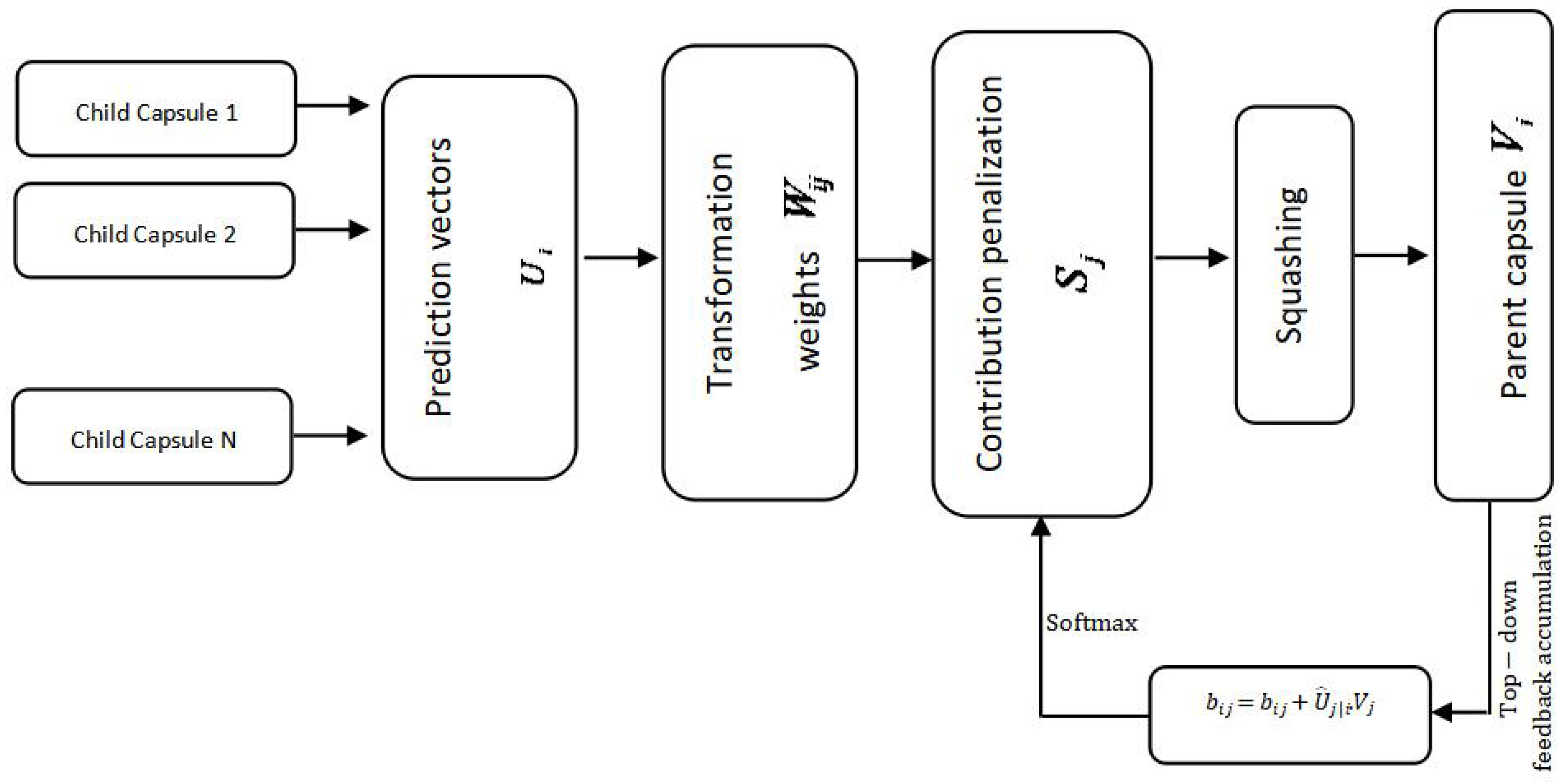
As mentioned previously, CNNs offer a high generalization capability in object recognition and detection tasks. However, their capability of modeling the relative positions of objects in an image is limited. Furthermore, the (standard) max-pooling operation omits fine details that could be informative for delicate image interpretation scenarios. Despite these limitations, CNNs offer a very good property of translating knowledge regarding the learned weights across the image and into a chain of layers. Therefore, the underlying insight characterizing CapsNets is to retain this property, while tackling the limitations of the CNNs mentioned above. CapsNets thus operate on convolutional feature maps generated from the image at hand. CapsNets consists of a set of capsules that receive knowledge about an entity (e.g., object part or object structure) from a preceding set of capsules (except for the first layer, which acquires convolutional maps of the image) and delivers a ‘prediction vector’ by multiplying its own output by a weight matrix. If the prediction vectors exhibit a large scalar product with the output of the potential parent capsule in the layer above, a top-down feedback is leveraged to magnify the coupling coefficient joining the current capsule with the possible parent capsule on the one hand, and shrink the coupling coefficients stemming into other potential parent capsules in the upper layer. This agreement-based routing perpetuates the likelihood of associating an object part with its main object as we ascend through the hierarchy.

A straightforward approach to quantify the presence of objects is appending a logistic unit to draw the probability of existence of a certain entity. However, in CapsNets, the length of the output vector of a capsule is converted into a probability, while its orientation is forced to accommodate the instantiation parameters (e.g., position, size, orientation, deformation, velocity, albedo, hue, texture) of the object or object part that the capsule is tied to. In order to scale down the length of the output vector while ensuring that its orientation remains unchanged, a non-linear squashing is applied as follows:

$$V_j=\frac{{\Vert S_j\Vert }^2}{1+{\Vert S_j\Vert }^2}\frac{S_j}{\Vert S_j\Vert }$$

(1)

where $V_j$ represents the vector output of capsule $j$ and $S_j$ is its total output. Thus, short vectors and long vectors are scaled down to almost zero and slightly below 1, respectively.

The total input to a capsule $S_j$ collects penalized contributions of prediction vectors ${\widehat{U}}_{j\vee i}$ emanating from the layers below by multiplying the output the previous layer capsules by a weight matrix $W_{ij}$ as follows:

$$S_j={\displaystyle {\sum }_i{C}_{ij}}{\widehat{U}}_{j|i}\mathrm{and}{\widehat{U}}_{j|i}=W_{ij}{U}_i$$

(2)

where $C_{ij}$ is the coupling coefficients between the capsule in the current layer and the capsule in the layer above which is determined via a top-down feedback through iterative dynamic routing. We want $C_{ij}$ to sum to 1. Therefore, a softmax unit is applied.

$$C_{ij}\frac{\exp (b_{ij})}{{\displaystyle \sum _k{b}_{ik}}}$$

(3)

where $b_{ij}$ is the initial logit, set as log prior probability, which represents the coupling between the current capsule and its potential parent above. Thus, it is learned by assessing the agreement between the output of the potential parent $V_j$ and the prediction vector ${\widehat{U}}_{j\vee i}$ generated by the capsule below (in the previous layer). The agreement is measured via a scalar product, and then accumulated to the initial logit as follows:

$$b_{ij}=b_{ij}+{\widehat{U}}_{{}_{j|i}}{V}_j$$

(4)

This refinement process permits the magnification of coupling coefficients between child and parent capsules that represent the same entity, and the decay of coefficients of capsules that are tied to irrelevant entities.

Figure 1 shows a graphical representation of the routing algorithm between two layers. We refer the readers to [41] for the detailed explanation on the routing algorithm.

2.2. Architecture

The basic architecture of the CapsNet, which is adopted in this work, is composed of two convolutional layers and one fully connected layer. The first convolutional layer, which is produced by 256 9 × 9 kernels with a stride of 1 and ReLU activation, delivers feature maps that are further fed to the primary set of capsules in the layer above.

The second layer represents the primary capsules, and accommodates 32 channels, thus 8D convolutional capsules of 9 × 9 kernels and a stride of 2, where each capsule captures all the units in the first convolutional layer whose receptive fields overlap with the center of the capsule. Thus, the set of primary capsules outputs a total of 32 × 6 × 6 8D vectors, and the capsules of the same grid share their weights with each other. The last layer of the CapsNet is a fully connected layer of 2 16D units that are connected to all the capsules in the previous layer.

Since the output of first convolutional layer is one dimensional, it does not convey the same quality of information as the capsules in the layer above (i.e., the output of the first layer does not provide orientation attributes to agree upon), no routing is envisioned with the primary capsules. It is noteworthy that all the logits $b_{ij}$ are initialized as zero, which implies that the initial capsule output is sent to all potential parent capsules with equal probability $C_{ij}$. In other words, prior to knowledge optimization, the primary capsules assume an equal agreement with parent capsules (e.g., all the entities tied with primary capsules are likely associated to the entities tied to the parent capsules above).

With regards to the loss function for the network to learn, it consists in increasing the length of the instantiation vector $V_k$ for an entity class (car and solar panel in our case) only if that particular entity is indeed observed in the image. This can be extended for multiple entities by using a separate margin loss $L_k$ for each entity capsule $k$:

$$L_k=T_k\max {(0,m^{+}-\Vert V_k\Vert )}^2+\lambda (1-T_k)\max {(0,\Vert V_k\Vert -m^{-})}^2$$

(5)

where $T_k$ is set to one if the entity is present and $m^{+}=0.9,m^{-}=0.1$ are fixed thresholds, $\lambda =0.5$ is a down-weighting of the loss for absent object classes. It is worth-mentioning that the number of routing iterations is set to three as in [41] with a batch size of 16. The learning rate is set to 0.001.

2.3. Image Reconstruction

In order to rebuild the input image of a certain entity, the activity vectors, except the one associated to the entity of interest, are masked. Then, the output of the correct capsule is fed into a decoder of 3 fully connected layers, and the squared differences between the outputs of the logistic units and the pixel intensities are minimized. This loss is scaled down by 5.10⁻⁴ to prevent it from dominating the margin loss during the training phase. The architecture of the CapsNet, as well as the reconstruction module, are given in [41].

3. Experimental Results

The following two subsections describe the datasets and experimental setup, and present experimental results with a detailed analysis on different CapsNet configurations.

3.1. Dataset Description and Design of Experiments

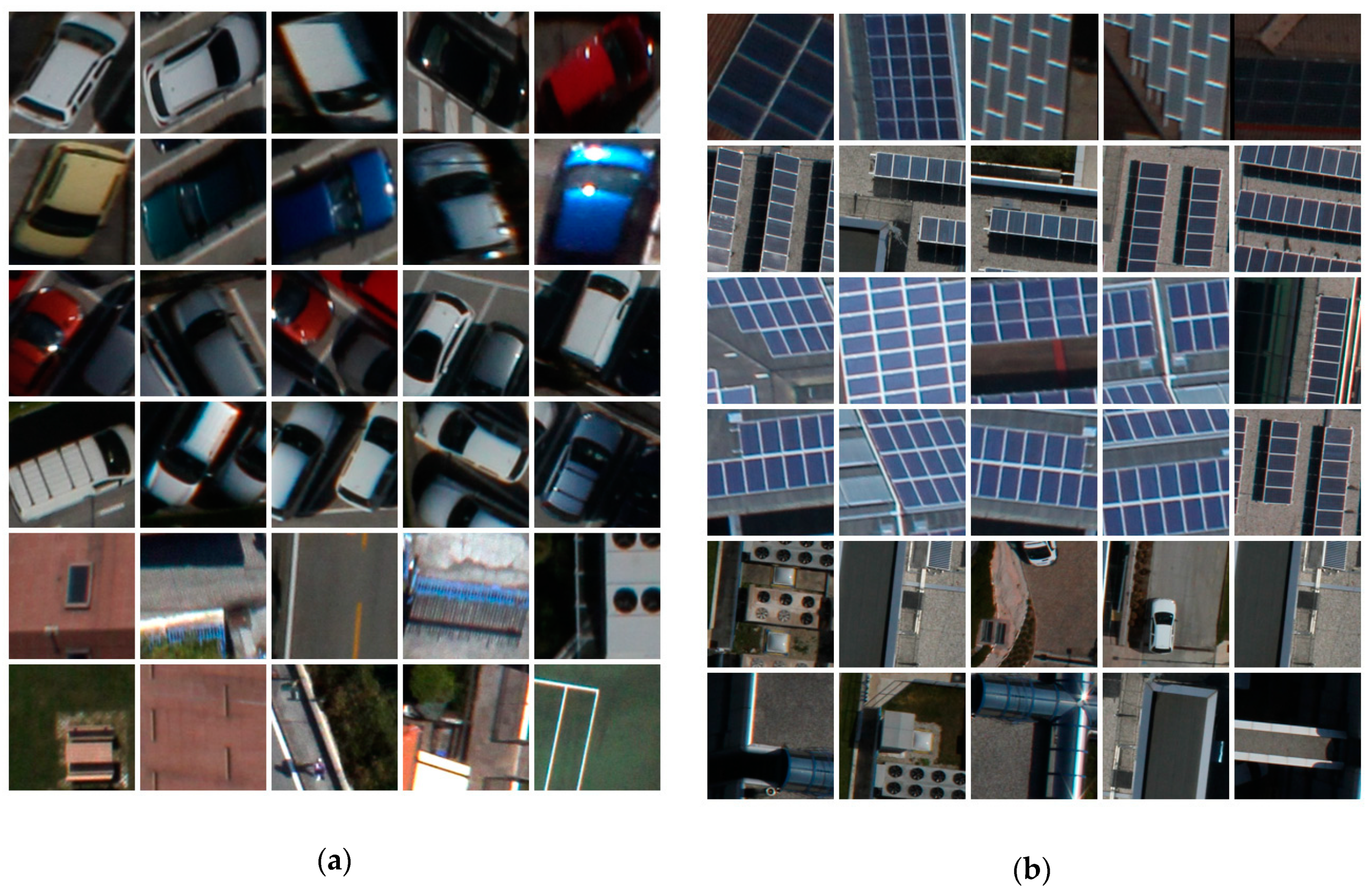
We evaluated the CapsNet on two UAV datasets, which were acquired over different areas on the city of Trento, Italy by a Canon EOS 550D camera (which includes CMOS APS-C sensor with 18 megapixels) mounted on an UAV. Both datasets include images in the red-green-blue (RGB) color space that have a spatial resolution of roughly 2 cm and a radiometric resolution of 8 bits. For both datasets, the pixel size of the images is 224 × 224. The first dataset is the car dataset (see Figure 2a). Vehicle detection and counting constitutes a vital part of urban planning, especially in dense metropolitan cities. Having an accurate estimate of cars either on-road or in parking lots can help avoid traffic congestion and better space allocation, especially during peak hours. The training set consists of 200 images (100 images include cars, while 100 images do not include cars) that were acquired over two parking lots in the city of Trento. The test set comprises 1000 images (500 images include cars, while 500 images do not include cars) that were acquired over three parking lots on the city of Trento. The second dataset is the solar panel dataset (see Figure 2b). Clean sustainable energy is arguably one of the most discussed issues since the late ‘Paris Agreement’ [42]. Solar panels offer a cheap source of green energy in the long run. Thus, solar panel detection can play a pivotal role towards drawing an accurate solar panel distribution and planning, particularly in dense residential cities. Similar to the car dataset, the training set consists of 200 images (100 images include solar panels, while 100 images do not include solar panels). The test set comprises 1000 images (500 images include solar panels, while 500 images do not include solar panels).

It is worth noting that all the images of both datasets were acquired over different time spans under different acquisition conditions and thus they represent challenging object detection problems. In the experiments, the pixel size of the images was down-sampled to 28 × 28 for both datasets. Since we are addressing a binary classification problem, the number of output activation vectors is two, whereas the dimension of the final layer is retained as 16. The first convolutional layer applies a 9 × 9 × 3 filter in order to take into account the input with all the three channels of the images. Our code has been implemented in Python via TensorFlow on a NVIDIA GPU GEFORCE GTX 960 M with 4GB RAM. The CapsNet has been trained with Adam Optimizer initialized with the default parameters and a batch size of 16. The same loss function suggested in the original paper was used, and thus m+ = 0.9, m− = 0.1 and λ = 0.5. The dynamic routing algorithm performs three iterations as suggested in [43]. The accuracy of correctly classified test images over the total number of test images is considered as evaluation metric.

3.2. Experimental Results

A. Sensitivity Analysis with respect to different parameter settings and strategies

In this subsection, we carried out different kinds of experiments in order to assess the impact of the convolutional kernel size, the parameters of the primary caps, the length of activation vectors and adding an extra hidden layer.

A paramount parameter in the network is the size of the filters adopted in the convolutional as well as the PrimaryCaps layers, since their size decides the spot in the input image to analyse, which is related to the features learned by the network (thus to the classification accuracy). Therefore, we study the impact of the following filter sizes: 3 × 3, 5 × 5, 7 × 7, 9 × 9 and 11 × 11 in both layers. The results are reported in

Table 1. Analysis of the filter size of the Conv layer versus the accuracy (in %): Left: Car dataset, Right: Solar Panel dataset.

	Filter size
	3 × 3	5 × 5	7 × 7	9 × 9	11 × 11
Car dataset	94.95	95.36	95.26	95.06	94.25
Solar Panel dataset	93.64	91.73	89.91	98.21	88.2

.

The results of Table 1 indicate that, in general, increasing the filter size reduces the accuracy except for the filter size of 3 × 3 on the Car dataset, which is due to initialization. This is likely traced back to the fact that small-sized kernels capture finer details in the Conv layer, which are further propagated among the capsules for strengthening the agreement with potential upper capsules.

The behavior of the primary caps that can significantly affect the performance of the CapsNet depends on three parameters: (i) filter size, (ii) depth (i.e., number of channels in primary caps) and (iii) dimension of the output vectors.

Table 2. Analysis of filter size versus accuracy in primary caps layer (in %): Left: Car dataset, Right: Solar Panel dataset.

	Filter size
	3 × 3	7 × 7	11 × 11
Car dataset	95.36	95.66	95.96
Solar Panel dataset	92.23	92.54	93.54

compares the filter size versus accuracy obtained for the two datasets. The results show that slight improvements are observed when the filter size increases.

We also evaluated the effect of the number of channels in primary caps. We recall that the original architecture of CapsNet uses 32 channels of 8D capsules in order to cover up the 256 feature maps of the Conv layer.

Table 3. Accuracy versus the number of channels in primary caps: Left: Car dataset, Right: Solar Panel dataset.

	Number of channels
	8	16	32	48
Car dataset	94.65	95.86	95.96	95.86
Solar Panel dataset	93.04	93.04	93.64	93.95

shows that, in general, increasing the number of channels introduces improvements. However, it is worth noting that this might cause the network to overfit the data.

We also assessed the length of output vectors in the primary caps. It is worth noting that the output vectors encode various instantiation parameters, which implies that their length is determined based on the problem at hand. Thus, objects that exhibit a wide range of changes might require a long vector in order to properly encode their behavior, whereas objects that remain stable in different observations across several images would require shorter instantiation arrays. This issue is shown in

Table 4. Accuracy versus the length of output vectors in primary caps: Left: Car dataset, Right: Solar Panel dataset.

	Length of output vectors
	4	8	12	16	20
Car dataset	95.86	95.96	96.06	96.47	95.76
Solar Panel dataset	93.34	93.65	93.34	93.24	93.75

, where the accuracy fluctuates as the length of the output vectors changes.

Since we deal with a binary classification problem, two (one for each class) OutputCaps of 16D each are envisioned. However, the length of the activation vectors is worth of investigation. We opt for the following lengths 8, 12, 16, 20 and 24, and the respective results are given in

Table 5. Analysis of the length of activation vectors: Left: Car dataset, Right: Solar Panel dataset.

	Length of activation vectors
	8	12	16	20	24
Car dataset	96.16	96.27	96.47	96.27	95.46
Solar Panel dataset	93.24	93.54	93.95	93.44	93.24

.

It can be observed that for both datasets, the trend of the accuracy is comparable overall, since it increases up to the vector length of 16 and slightly declines afterwards. At this point, increasing the vector length offers too much space to encode the information received from the layer below. Similarly, shrinking the vector length does not seem to be enough to encode such information either. A trade-off between the two extremes, 16D activation vectors in both datasets, remains an optimal option.

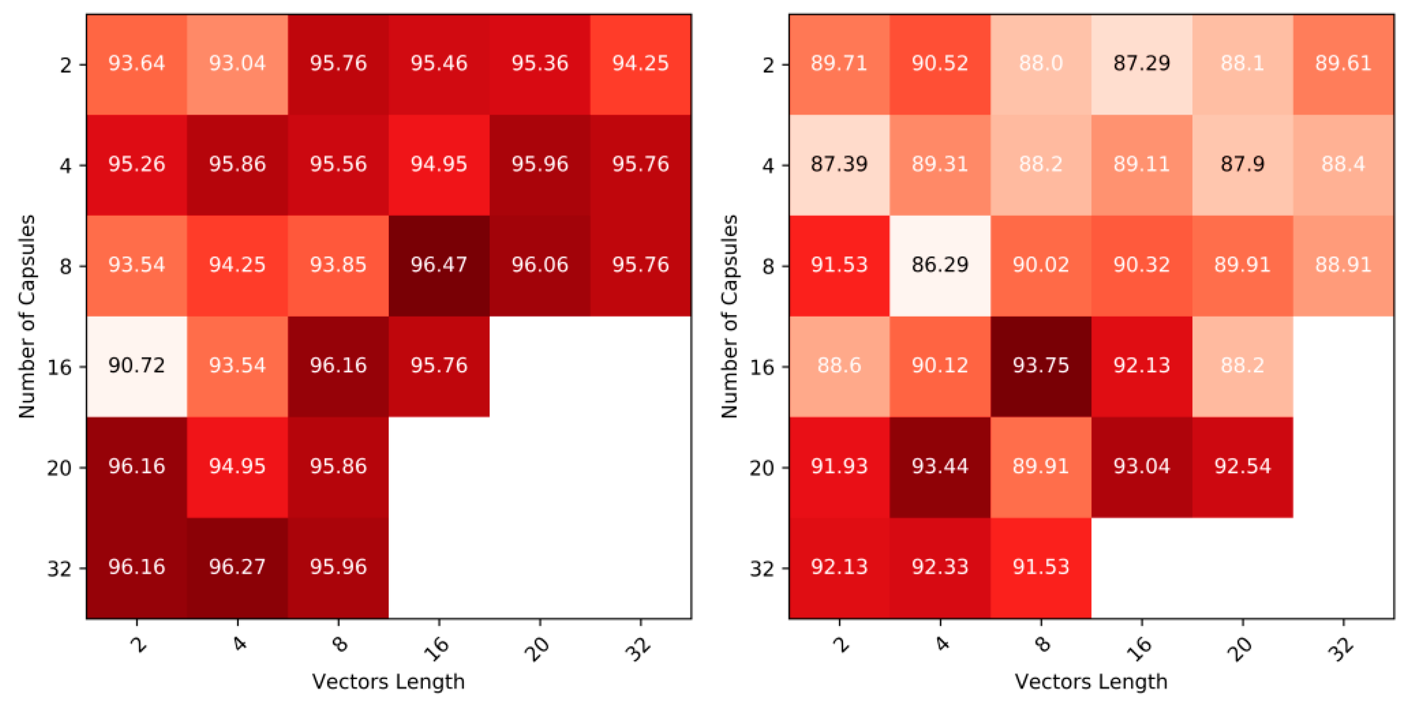
Adding more layers to the network may inflate the processing load, notwithstanding the potential to overfit the training data. If both scenarios are well-approached, classification gains might be envisioned, since deeper features convey richer information. Thus, we study the behavior of the network when an extra Caps layer is added. Therefore, two parameters are to be assessed (i) number of capsules and (ii) the length of the output vectors in these capsules. Figure 3 provides a heatmap of the accuracy in terms of both parameters (white cells represent cases that the capacity of the adopted GPU could not handle).

It can be noted that the number of Caps exhibits a larger impact than the length of the output vectors. This might be explained by the reason that capsules are tied to entities (partial/full objects), which seems to be more significant in our datasets than the length of the vectors that encodes the instantiation of the entities.

B. Comparison of the CapsNet with the State-of-the-Art Methods

In this subsection, we address a cross-dataset transfer learning scenario. Therefore, we consider the case when the Car and Solar Panel datasets are utilized interchangeably for training and test. Afterwards, we compare the CapsNet with the state-of-the-art methods applied to the same datasets.

Given that the Car and the Solar Panel datasets are acquired by the same sensor, it is possible for a network that was trained on the one dataset to be applied to the other dataset. This is a paramount process in real applications as it can save time and resources when dealing with large scale data. In details, we train a CapsNet on the Car datasets with the following parameters: image size of 36 × 36, 5 × 5 Conv layer filer, PrimaryCaps of 11 × 11 filers and 32 channels 16D output vectors, 16D activation vectors, and then apply it on the Solar Panel dataset. Then, the same architecture is trained on the Solar Panel dataset and applied on the Car dataset. The results are reported in

Table 6. Accuracies and processing time (in sec) obtained with and without applying transfer learning on the Solar Panel dataset.

	Trans. Learning	Without Trans. Learn.
Accuracy (in %)	90.82	91.73
Processing Time (in sec)	7.6	7.6

and

Table 7. Accuracies and processing time (in sec) obtained with and without applying transfer learning on the Car dataset.

	Trans. Learning	Without Trans. Learn.
Accuracy (in %)	95.86	95.76
Processing Time (in sec)	6.5	6.5

.

From the Tables, one can see that transfer learning is comparable to the traditional case in terms of both accuracy and processing time. On the one hand, this might be due to the fact that the images were acquired by the same sensor. On the other hand, the Car and the Solar Panel datasets share some similarities in terms of shape (i.e., rectangular). Furthermore, the negative samples in both datasets have a certain similarity.

One of the main properties of CapsNet is that the classification paradigm is embedded in the architecture itself, by relying on the length of the activation vectors. However, it would be interesting to consider CapsNet for feature extraction only. Therefore, we considered a support vector machines (SVM) classifier (with RBF kernel) placed at different positions (i.e., fed with the features of the primary caps, and then with the features of the output caps) within the network. The parameters of the SVM (the penalization parameter and the kernel parameter) were optimized by means of a cross-validation strategy on the training set with a split of 50/50 percent. On this point, we consider two scenarios, namely (i) the original architecture and (ii) adding another hidden layer.

By analyzing the

Table 8. Classification accuracies (%) obtained by the CapsNet and the support vector machines (SVM) classifier fed with features from different layers of the network.

Dataset/Scenario	CapsNet	SVM Fed with Primary Caps Features	SVM Fed with Output Caps Features
Car	96.47	59.4	96.1
Solar Panel	93.95	75.6	93.9

one can see that accuracies obtained by SVM are slightly smaller than those of the CapsNet when the features of the output caps are used, and significantly smaller when the features of the primary caps are adopted. Moreover, using the embedded classifier of CapsNet lifts the need to tune up extra parameters (which is the case of the SVM). We also draw the attention to the poor performance of the Primary Caps features, which is expected since the network, at this layer, has not matured discriminative features with respect to the output layer. However, the results reported in

Table 9. Classification accuracies (%) obtained by the CapsNet and the SVM classifier fed with features from different layers of the network with an extra hidden layer.

Dataset/Scenario	CapsNet	SVM Fed with Primary Caps Features	SVM Fed with Hidden Caps Features	SVM Fed with Output Caps Features
Car	96.47	93.3	96.4	96.2
Solar Panel	93.75	93.1	93.2	93.8

suggest that adding a hidden layer stimulates the primary caps (via routing by agreement) and thus generates more meaningful representations.

In order to compare the CapsNet with the state-of-the-art methods, we consider several well-known CNN models, namely ResNet-50, ResNet-152, GoogLeNet, VGG16, VGGM, AlexNet. We also compare our work with a recent paper, which presents a Convolutional SVM (CSVM) [44] on the same datasets. Results regarding training time, testing time and accuracy are summarized in

Table 10. Comparison with the state-of-the-art on the Car dataset.

	ResNet-50	ResNet-152	GoogLeNet	VGG16	VGGM	AlexNet	CSVM (11 × 11, 5 × 5, 3 × 3, 1 × 1, 1 × 1) [44]	CSVM (7 × 7, 1 × 1, 3 × 3, 1 × 1, 1 × 1) [44]	CapsNet
Accuracy (%)	91.10	90.05	94.74	95.66	88.34	91.93	95.78	97	96,47
Train/Test time (Sec)	75/274	270/1220	126/510	235/976	45/212	42/161	130/9	185/12	221/8,8

and

Table 11. Comparison with the state-of-the-art on the Solar Panel dataset.

	ResNet-50	ResNet-152	GoogLeNet	VGG16	VGGM	AlexNet	CSVM (11 × 11, 5 × 5, 3 × 3, 1 × 1, 1 × 1) [44]	CSVM (7 × 7, 1 × 1, 3 × 3, 1 × 1, 1 × 1) [44]	CapsNet
Accuracy (%)	66.43	66.37	84.45	93.59	95.45	93.01	96.24	96.97	93,95
Train/Test time (Sec)	81/396	289/1300	102/509	201/988	45/213	40/154	120/10	156/12	111/4

. The scores indicate that CapsNet yields comparable results to the aforementioned baselines in terms of accuracy on both datasets, except for the Solar Panel dataset where CSVM remains better. Regarding the processing time (test phase). However, CapsNet is the fastest among all, since it does not accumulate the feature maps over a long chain of layers. Thus, CapsNet is much more suitable to be used on real operational object detection scenarios.

5. Conclusions

This paper has presented a Capsule Networks (CapsNet) framework for object detection in UAV-acquired images. Unlike usual deep models such as CNNS (which capitalize on the depth aspect and omit the object’s relative position), CapsNet consists of a simple shallow architecture that can detect complex objects under challenging scenarios thanks to the routing by agreement strategy, which enables the spread of objects relative position within an image across several layers. This further lessens the processing overheads with respect to CNNs.

Experiments conducted on two UAV-acquired datasets of cars and solar panels show that CapsNet can detect objects effectively. Moreover, owing to its shallow architecture, CapsNet runs in a shorter processing time as compared to recent deep models in the literature. This property is favoured in real-time object detection scenarios.

Another property of the CapsNet is that it could be used as a feature reconstruction module. Potentially, it could benefit other areas of remote sensing such as cloud removal and area reconstruction.

References

- Holness, C.; Matthews, T.; Satchell, K.; Swindell, E.C. Remote sensing archeological sites through Unmanned Aerial Vehicle (UAV) imaging. In Proceedings of the IEEE International Geoscience and Remote Sensing Symposium, Beijing, China, 10–15 July 2016; pp. 6695–6698. [Google Scholar]
- Malek, S.; Bazi, Y.; Alajlan, N.; AlHichri, H.; Melgani, F. Efficient framework for palm tree detection In UAV images. IEEE J. Sel. Top. Appl. Earth Obs. Remote Sens. 2014, 7, 4692–4703. [Google Scholar] [CrossRef]
- Niethammer, U.; James, M.R.; Rothmund, S.; Travelletti, J.; Joswig, M. UAV-based remote sensing of the Super-Sauze landslide: Evaluation and results. Eng. Geol. 2012, 128, 2–11. [Google Scholar] [CrossRef]
- Berni, J.A.; Zarco-Tejada, P.J.; Suárez, L.; Fereres, E. Thermal and narrowband multispectral remote sensing for vegetation monitoring from an unmanned aerial vehicle. IEEE Trans. Geosci. Remote Sens. 2009, 47, 722–738. [Google Scholar] [CrossRef]
- Lin, A.Y.M.; Novo, A.; Har-Noy, S.; Ricklin, N.D.; Stamatiou, K. Combining GeoEye-1 satellite remote sensing, UAV aerial imaging, and geophysical surveys in anomaly detection applied to archaeology. IEEE J. Sel. Top. Appl. Earth Obs. Remote Sens. 2011, 4, 870–876. [Google Scholar] [CrossRef]
- Zhou, C.; Yang, G.; Liang, D.; Yang, X.; Xu, B. An Integrated Skeleton Extraction and Pruning Method for Spatial Recognition of Maize Seedlings in MGV and UAV Remote Images. IEEE Trans. Geosci. Remote Sens. 2018, 56, 4618–4632. [Google Scholar] [CrossRef]
- Everaerts, J. In The use of unmanned aerial vehicles (UAVs) for remote sensing and mapping. ISPRS Int. Arch. Photogramm., Remote Sens. Spat. Inf. Sci. 2008, 38, 1187–1192. [Google Scholar]
- Remondino, F.; Barazzetti, L.; Nex, F.; Scaioni, M.; Sarazzi, D. In UAV photogrammetry for mapping and 3D modeling–current status and future perspectives. ISPRS Int. Arch. Photogramm., Remote Sens. Spat. Inf. Sci. 2011, 38, 25–31. [Google Scholar] [CrossRef]
- Watts, A.C.; Ambrosia, V.G.; Hinkley, E.A. Unmanned aircraft systems in remote sensing and scientific research: Classification and considerations of use. Remote Sens. 2012, 4, 1671–1692. [Google Scholar] [CrossRef]
- Crommelinck, S.; Bennett, R.; Gerke, M.; Nex, F.; Yang, M.Y.; Vosselman, G. Review of automatic feature extraction from high-resolution optical sensor data for UAV-based cadastral mapping. Remote Sens. 2016, 8, 689. [Google Scholar] [CrossRef]
- Melgani, F.; Bruzzone, L. Classification of hyperspectral remote sensing images with support vector machines. IEEE Trans. Geosci. Remote Sens. 2004, 42, 1778–1790. [Google Scholar] [CrossRef] [Green Version]
- Du, P.; Xia, J.; Zhang, W.; Tan, K.; Liu, Y.; Liu, S. Multiple classifier system for remote sensing image classification: A review. Sensors 2012, 12, 4764–4792. [Google Scholar] [CrossRef]
- Tuia, D.; Volpi, M.; Copa, L.; Kanevski, M.; Munoz-Mari, J. A survey of active learning algorithms for supervised remote sensing image classification. IEEE J. Sel. Top. Appl. Earth Obs. Remote Sens. 2011, 5, 606–617. [Google Scholar] [CrossRef]
- Zhang, L.; Zhang, L.; Tao, D.; Huang, X. On combining multiple features for hyperspectral remote sensing image classification. IEEE Trans. Geosci. Remote Sens. 2012, 50, 879–893. [Google Scholar] [CrossRef]
- Mekhalfi, M.L.; Melgani, F.; Bazi, Y.; Alajlan, N. Land-use classification with compressive sensing multifeature fusion. IEEE Geosci. Remote Sens. Lett. 2015, 12, 2155–2159. [Google Scholar] [CrossRef]
- Jiang, J.; Chen, C.; Yu, Y.; Jiang, X.; Ma, J. Spatial-aware collaborative representation for hyperspectral remote sensing image classification. IEEE Geosci. Remote Sens. Lett. 2017, 14, 404–408. [Google Scholar] [CrossRef]
- Hong, D.; Yokoya, N.; Zhu, X.X. Learning a robust local manifold representation for hyperspectral dimensionality reduction. IEEE J. Sel. Top. Appl. Earth Obs. Remote Sens. 2017, 10, 2960–2975. [Google Scholar] [CrossRef]
- Hong, D.; Yokoya, N.; Chanussot, J.; Zhu, X.X. An augmented linear mixing model to address spectral variability for hyperspectral unmixing. IEEE Trans Image Process. 2018, 28, 1923–1938. [Google Scholar] [CrossRef]
- Moranduzzo, T.; Mekhalfi, M.L.; Melgani, F. LBP-based multiclass classification method for UAV imagery. In Proceedings of the IEEE International Geoscience and Remote Sensing Symposium, Milan, Italy, 26–31 July 2015; pp. 2362–2365. [Google Scholar]
- Moranduzzo, T.; Melgani, F.; Mekhalfi, M.L.; Bazi, Y.; Alajlan, N. Multiclass coarse analysis for UAV imagery. IEEE Trans. Geosci. Remote Sens. 2015, 53, 6394–6406. [Google Scholar] [CrossRef]
- Al Rahhal, M.; Bazi, Y.; Abdullah, T.; Mekhalfi, M.; AlHichri, H.; Zuair, M. Learning a Multi-Branch Neural Network from Multiple Sources for Knowledge Adaptation in Remote Sensing Imagery. Remote Sens. 2018, 10, 1890. [Google Scholar] [CrossRef]
- Zhou, B.; Lapedriza, A.; Xiao, J.; Torralba, A.; Oliva, A. Learning deep features for scene recognition using places database. In Proceedings of the Advances in Neural Information Processing Systems, Montreal, QC, Canada, 8–13 December 2014; pp. 487–495. [Google Scholar]
- Ahmad, K.; Mekhalfi, M.L.; Conci, N.; Melgani, F.; Natale, F.D. Ensemble of Deep Models for Event Recognition. ACM Trans. Multimed. Comput. 2018, 14, 51. [Google Scholar] [CrossRef]
- Qi, C.R.; Su, H.; Mo, K.; Guibas, L.J. Pointnet: Deep learning on point sets for 3d classification and segmentation. In Proceedings of the Computer Vision and Pattern Recognition, Kauai, HI, USA, 21–26 July 2017; pp. 652–660. [Google Scholar]
- Diao, W.; Sun, X.; Zheng, X.; Dou, F.; Wang, H.; Fu, K. Efficient saliency-based object detection in remote sensing images using deep belief networks. IEEE Geosci. Remote Sens. Lett. 2016, 13, 137–141. [Google Scholar] [CrossRef]
- Zhang, Y.; Li, X.; Zhang, Z.; Wu, F.; Zhao, L. Deep learning driven blockwise moving object detection with binary scene modeling. Neurocomputing. 2015, 168, 454–463. [Google Scholar] [CrossRef]
- Lin, K.; Yang, H.F.; Hsiao, J.H.; Chen, C.S. Deep learning of binary hash codes for fast image retrieval. In Proceedings of the IEEE Conference on Computer Vision and Pattern Recognition Workshops, Boston, MA, USA, 11–12 June 2015; pp. 27–35. [Google Scholar]
- Gordo, A.; Almazán, J.; Revaud, J.; Larlus, D. Deep image retrieval: Learning global representations for image search. In Proceedings of the European Conference on Computer Vision, Amsterdam, The Netherlands, 8–16 October 2016; pp. 241–257. [Google Scholar]
- Zhang, L.; Zhang, L.; Du, B. Deep learning for remote sensing data: A technical tutorial on the state-of-the-art. IEEE Geosci. Remote Sens. Mag. 2016, 4, 22–40. [Google Scholar] [CrossRef]
- Penatti, O.A.; Nogueira, K.; dos Santos, J.A. Do deep features generalize from everyday objects to remote sensing and aerial scenes domains? In Proceedings of the IEEE Conference on Computer Vision and Pattern Recognition Workshops, Boston, MA, USA, 11–12 June 2015; pp. 44–51. [Google Scholar]
- Chen, Y.; Lin, Z.; Zhao, X.; Wang, G.; Gu, Y. Deep learning-based classification of hyperspectral data. IEEE J. Sel. Top. Appl. Earth Obs. Remote Sens. 2014, 7, 2094–2107. [Google Scholar] [CrossRef]
- Kussul, N.; Lavreniuk, M.; Skakun, S.; Shelestov, A. Deep learning classification of land cover and crop types using remote sensing data. IEEE Geosci. Remote Sens. Lett. 2017, 14, 778–782. [Google Scholar] [CrossRef]
- Krizhevsky, A.; Sutskever, I.; Hinton, G.E. Imagenet classification with deep convolutional neural networks. In Proceedings of the Advances in Neural Information Processing Systems, Harrah’s Lake Tahoe, CA, USA, 3–8 December 2012; pp. 1097–1105. [Google Scholar]
- Chatfield, K.; Simonyan, K.; Vedaldi, A.; Zisserman, A. Return of the devil in the details: Delving deep into convolutional nets. arXiv 2014, arXiv:1405.3531. [Google Scholar]
- He, K.; Zhang, X.; Ren, S.; Sun, J. Deep residual learning for image recognition. In Proceedings of the IEEE Conference on Computer Vision and Pattern Recognition, Las Vegas, CA, USA, 26 June–1 July 2016; pp. 770–778. [Google Scholar]
- Szegedy, C.; Liu, W.; Jia, Y.; Sermanet, P.; Reed, S.; Anguelov, D.; Rabinovich, A. Going deeper with convolutions. In Proceedings of the IEEE Conference on Computer Vision and Pattern Recognition, Boston, CA, USA, 8–10 June 2015; pp. 1–9. [Google Scholar]
- Simonyan, K.; Zisserman, A. Very deep convolutional networks for large-scale image recognition. arXiv 2014, arXiv:1405.3531. [Google Scholar]
- Li, K.; Cheng, G.; Bu, S.; You, X. Rotation-insensitive and context-augmented object detection in remote sensing images. IEEE Trans. Geosci. Remote Sens. 2017, 56, 2337–2348. [Google Scholar] [CrossRef]
- Cheng, G.; Zhou, P.; Han, J. Learning rotation-invariant convolutional neural networks for object detection in VHR optical remote sensing images. IEEE Trans. Geosci. Remote Sens. 2016, 54, 7405–7415. [Google Scholar] [CrossRef]
- Cheng, G.; Han, J.; Zhou, P.; Xu, D. Learning rotation-invariant and fisher discriminative convolutional neural networks for object detection. IEEE Trans Image Process. 2018, 28, 265–278. [Google Scholar] [CrossRef]
- Sabour, S.; Frosst, N.; Hinton, G.E. Dynamic routing between capsules. In Proceedings of the Advances in Neural Information Processing Systems, Long Beach, NV, USA, 4–9 December 2017; pp. 3856–3866. [Google Scholar]
- The Paris Agreement. Available online: https://unfccc.int/process-and-meetings/the-paris-agreement/the-paris-agreement (accessed on 22 October 2018).
- Hinton, G.E.; Sabour, S.; Frosst, N. Matrix capsules with EM routing. In Proceedings of the International Conference on Learning Representations, Vancouver, BC, Canada, 30 April–3 May 2018. [Google Scholar]
- Bazi, Y.; Melgani, F. Convolutional SVM Networks for Object Detection in UAV Imagery. IEEE Trans. Geosci. Remote Sens. 2018, 56, 3107–3118. [Google Scholar] [CrossRef]
Figure 1.
Abstract illustration of the routing by agreement algorithm.
Figure 2.
Examples of the images: (a) the car dataset, (b) the solar panel dataset. First four rows depict images that include objects of interest (car or solar panel), while last two rows show the images that do not contain them.
Figure 3.
Number of Caps in the hidden layer versus the length of their output vectors: Left: Car dataset, Right: Solar Panel dataset.