Multi-Resolution Weed Classification via Convolutional Neural Network and Superpixel Based Local Binary Pattern Using Remote Sensing Images

Abstract

Automatic weed detection and classification faces the challenges of large intraclass variation and high spectral similarity to other vegetation. With the availability of new high-resolution remote sensing data from various platforms and sensors, it is possible to capture both spectral and spatial characteristics of weed species at multiple scales. Effective multi-resolution feature learning is then desirable to extract distinctive intensity, texture and shape features of each category of weed to enhance the weed separability. We propose a feature extraction method using a Convolutional Neural Network (CNN) and superpixel based Local Binary Pattern (LBP). Both middle and high level spatial features are learned using the CNN. Local texture features from superpixel-based LBP are extracted, and are also used as input to Support Vector Machines (SVM) for weed classification. Experimental results on the hyperspectral and remote sensing datasets verify the effectiveness of the proposed method, and show that it outperforms several feature extraction approaches.

1. Introduction

Weeds have global impact on economy, environment, public welfare and livestock [1]. Hence, continuous weed monitoring and control are inevitable. There is a strong need for the development of automated systems that can correctly recognize weed categories at the right time to make weed control effective and efficient. Remote sensing is a powerful means to monitor land cover and has a great potential to provide weed mapping with the aid of advanced data analysis tools.

In the literature, several methods have been proposed to classify weed category using different sensors. The main idea of weed classification is to capture the image of the vegetation from the field, process it using different feature extraction methods and then characterize each category of crop and weed. It can be facilitated by removing sensing that provides wide coverage and frequent observations via Red-Green-Blue (RGB) images, multi-spectral images (MSI) or hyper-spectral images (HSI).

Extensive research has been conducted to identify each category of weed. Pixel-based classification methods have been used by researchers to differentiate the background from crops [2,3]. With the availability of high-resolution hyperspectral sensors, it is possible to deploy object-based classification methods [4,5]. Object-based weed classification incorporates both spatial and spectral information, which has several advantages compared to the pixel-based classification methods when only spectral information of the material is required. It can extract the shape and textural features of each category of weed to improve the separability between weeds and other vegetation.

RGB images have been broadly utilized for weed mapping since they are simple and easy to adopt [3,4,6,7,8,9,10]. A Support Vector Machine (SVM) was used with RGB images for the arrangement of maize crops and sunflowers [11], where spectral intensity, textures, shapes, and geometrical properties were the attributes used for the classification. RGB images were also exploited for grouping of the species [7,8]. The texture and color details were extracted using neural networks to improve discriminant capacity [9]. A learning tactic was applied, which relied on decision trees for identifying vegetation using RGB images [10]. Recently, home lawn weed detection system using deep learning was established [3] using synthetic RGB images. Synthetic RGB images were formed artificially to generate a large dataset for deep network training. Hung et al. [4] used Unmanned Aerial Vehicle (UAV) to capture high-resolution RGB images for recognition of three weed types via feature learning. All the above methods utilized color images containing three bands in the visible range. Using pixel-based classification methods, multispectral images were used for weed mapping [2]. Multispectral/hyperspectral images contain a large number of contiguous and narrow bands. Consequently, more comprehensive spectral features could also be extracted [12].

The most dominant texture descriptor is Local Binary Pattern (LBP) [13,14], which has been successfully applied to face recognition and texture classification [15,16,17,18]. The LBP operator is a powerful means of feature extraction since it is rotational-invariant [13]. The LBP model has also been applied to remote sensing image analysis based on both spectral and spatial information. The LBP model was combined with fuzzy C-means algorithms [19] for the classification of multispectral images. The authors in [20] proposed a modified texture descriptor using LBP operator for land use and land cover classification via very high-resolution satellite imagery. LBP and Gabor filters were utilized in a subset of bands from HSIs to generate a complete set of texture data [21]. These spatial features were then concatenated to perform scene classification. In this paper, the LBP operator is used as one of the components of the proposed method.

Superpixel segmentation has advanced an effective and economical strategy to present the arrangement of the spatial distribution of surface materials [22,23,24]. The simple linear iterative clustering (SLIC) algorithm proposed by Achanta et al. [24] has been widely used as a superpixel generation method in the field of remote sensing. In particular, SLIC algorithms combine similar neighboring pixels into superpixels, whose shapes and sizes are adaptable according to different spatial structure. There are several advantages of using superpixels such as noise removal, redundancy reduction, and computational load saving.

For extracting the spatial attributes within superpixels, Fang et al. [25] made use of the mean and weighted average filter. Li et al. [26] developed a superpixel-level sparse representation classification (SRC) structure for hyperspectral descriptions while Jia et al. [27] presented a multitask learning structure using superpixel for HSI classification. Based on superpixel and fuzzy logic, Chen et al. [28] proposed an improved framework for spectral and spatial classification. For HSI classification, He et al. [29] merged SVM and superpixel division. Hence, we exploit the benefits of superpixels for weed classification. Conventional computer vision-based weed classification systems have been developed that mainly rely on handcrafted features [30,31]. Recently, Convolutional Neural Network (CNN) have spurred the use of end-to-end learning for the weed classification [32,33] and for other areas in remote sensing [34,35] to deal with the inflexibility and limitation of handcrafted methods. CNN is applied for the classification of weeds using MSI and RGB datasets. CNN has the ability to discover and learn semantic features appropriate for the organization of weeds. Using deep CNN, Ref. [36] assessed individual biomass extents of numerous dissimilar kinds of crops. Using RGB + Near-Infrared Reflectance (NIR)descriptions, two different CNN designs for classifying crop and weed are utilized [37].

Recent developments show the importance of deep learning techniques for weed classification [12,38]. Cost-effective automatic weed classification can be done using UAV/airborne sensors. However, each UAV/airborne sensor captures images with its own specification. For example, the same weed can be captured at different altitudes with a different focal length, diameter of the sensor and hence different resolutions. It is difficult to extract features from multi-resolution images using methods that are designed for different image resolutions. This multi-resolution problem is addressed in this study, where an automated method using CNN with superpixel based LBP coding is proposed. This method combines the features from different levels, i.e., local texture features are extracted from superpixel based LBP method and mid- and high-level spatial and spectral features from CNN. To the best of our knowledge, the multi-resolution issue has not been addressed so far using remote sensing images.

The following novel contributions are propounded in this study:

• CNN’s are widely used for the classification and detection of different objects. However, it is the first time that CNN architecture with two dropout (DPO) and fully connected (FC) layers is investigated for the classification of weeds using HSI and MSI datasets.
• We combine mid-level and high-level of features extracted from different layers of CNN to form a rich feature representation for the classification of weeds.
• Local texture features from superpixels based LBP codes and CNN features are combined to improve weed separability from the multi-resolution remote sensing images.

The remainder of the paper is organised as follows: the proposed frameworks are described in Section 2. Dataset and implementation details, training strategy, experimental results and discussions are presented in Section 3. Section 4 concludes all the experiments and research findings.

2. Methodology

To deal with the challenging issue of multi-resolution images of weeds, this paper integrates CNN with superpixel treatments, LBP operator and SVM. The proposed architecture is shown in Figure 1.

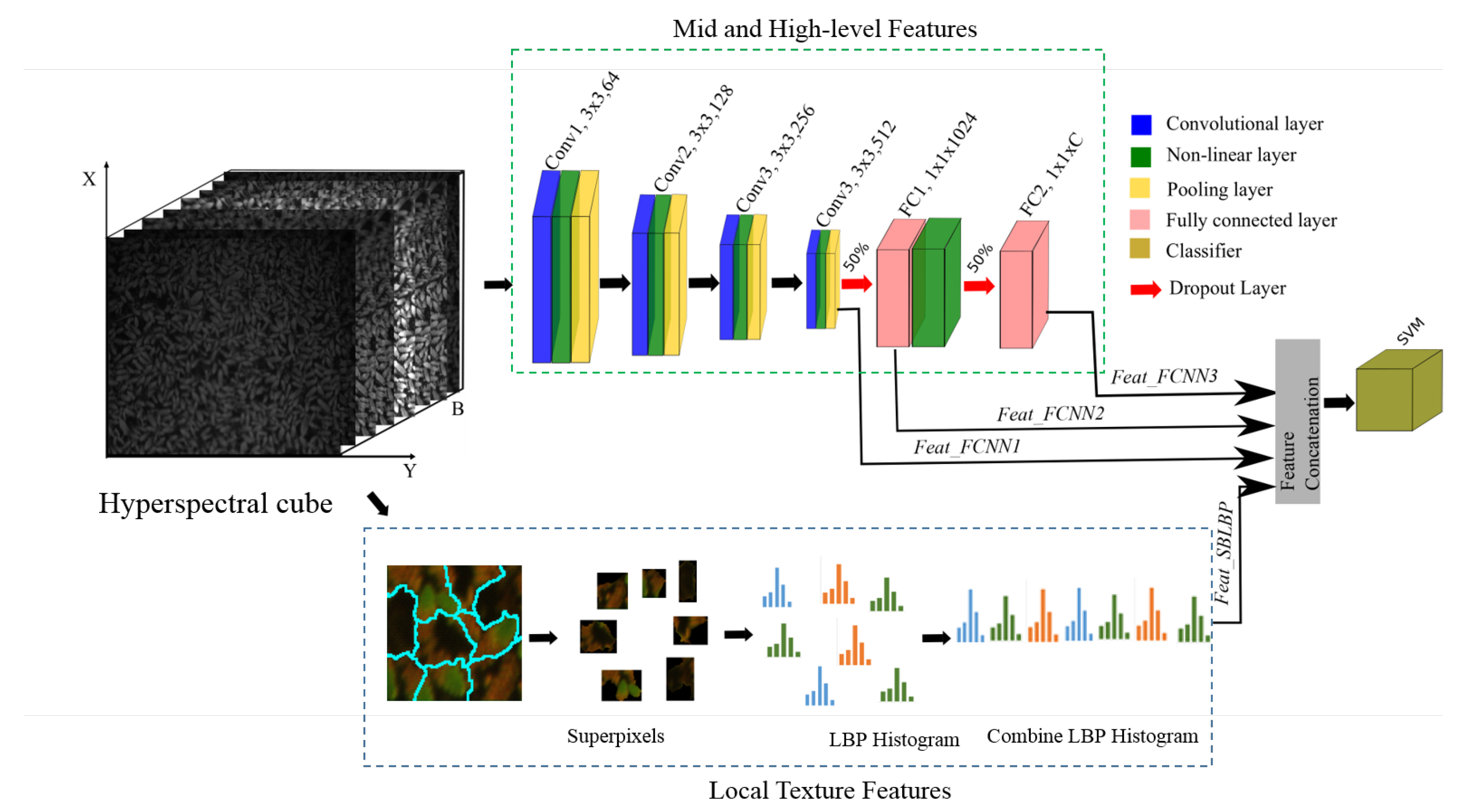
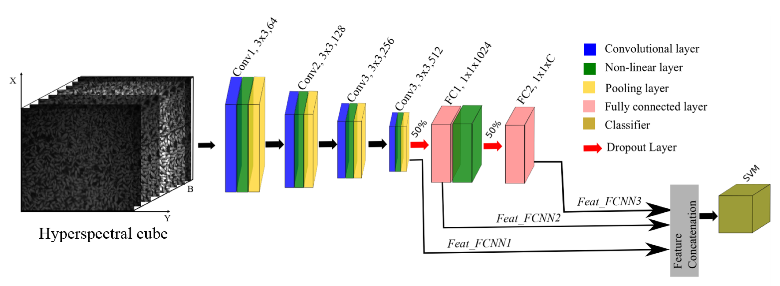
2.1. Multi-Layer Fused Convolution Neural Network (FCNN)

CNN lies in one of the categories of artificial neural networks that has been successfully adapted to understand the visual imagery [39]. CNN architectures are commonly designed by gathering various convolutional layers, pooling layers, and nonlinearity layers. This hierarchy allows the CNN’s network to learn the data at multiple levels. Low-level features, such as edges and corners, are extracted from the bottom layers, and high-level semantic information is taken out from the top layers. CNN has the advantage of internal connection between each layer and weight sharing which helps the CNN architecture to achieve state-of-the-art results in Computer Vision and Natural Language Processing.

For weed classification, multi-resolution weed images with 2D structure are the CNN inputs. Then, 2D convolutional filters are applied. The size of input images to CNN architecture is $W_t\times H_t$ pixels. Each convolutional layer of the CNN architecture can be defined as follows:

$$F_{map}^W=\sum _{n=1}^D{W}_n\ast I^n+b,$$

(1)

where I is the image or the feature map of the previous layer of size $W_t\times H_t\times D$ and filter bank W of size $w\times h\times D$, * is the discrete convolutional operator, b corresponds to the trainable bias parameters and $F_{map}$ is the feature map of convolutional layer.

To introduce the nonlinearity in the model, the activation function is used. The most commonly used activation function after each convolutional layer is the rectified linear unit (ReLU). The ReLU layer consists of a nonlinearity function and is applied to the output of convolutional layer $F_{map}$. This nonlinearity layer can be computed as:

$$F_{NL}=f\left(F_{map}\right),$$

(2)

where $f(.)$ is defined as $f\left(x\right)=max(0,x)$.

This nonlinearity layer sets all the negative numbers in the convolution matrix to zero while the positive numbers remain unchanged. To make the features robust against the distortion and noise, a pooling layer is adopted. Max pooling function has successfully been used in the literature after the activation layer. On each feature map, max operation is applied on spatial regions G as follows:

$$F_{PL}=\underset{i\in G}{max}{F}_{N{L}_i}.$$

(3)

CNN has the limitation of over-fitting and one way to avoid this is by having large training samples. There are, however, limited data available in remote sensing. In this paper, the data set is increased by data augmentation methods. Well-known and effective data augmentation methods [12], such as random cropping and rotation, are used to increase the data sets. The performance of the classifier depends upon the weight and bias parameters. Therefore, to find weights and biases that will minimize the error (i.e., minimizing the predicted values and the target values), the loss function is penalized by the misclassifications. The most commonly used loss function is the cross-entropy loss function:

$$\mathcal{L}(x,t,p)=-\sum _i{t}_{i}logp\left(x_i\right).$$

(4)

Herein, a Stochastic Gradient Descent (SGD) with back-propagation algorithm [40] is used in the paper for optimization. Based on the comparison of different optimizers conducted in [41], we used an SGD optimizer with momentum.

As stated above, CNN is based on feature learning, where each layer is taught to extract different types of features. With a human eye, we initially recognize edges of some objects and, as it comes closer, we recognize the whole object. However, only a small amount of information is available for the middle layers of the human brain. Generally, features extracted from the middle layers are the mixture of low and high-level features that can be used to distinguish each category of weed. Zeiler and Fergus [42] and Lee et al. [43] visually demonstrated features of each layer. From that visualization, low-level features extracted from the earlier CNN layers are different from the low-level feature extracted from the hand-crafted methods because these methods were designed for only specific problems. However, features extracted from each layer of trained CNN are used to extract useful features for the given set of images. For instance, mid-level features are successfully used for object recognition in different areas of computer vision [44,45]. More class-specific features can be extracted using layers before the final layer(s) and more significant features of each class can be extracted using the final layer [42]. Hence, features are extracted from the final layer as well as from previous layers to have a more rich feature representation of each category of weed. The proposed model is shown in Figure 2. Extracted features from each layer is then concatenated to make a single feature vector as $Feat\_FCNN=\left[Feat\_FCNN1,Feat\_FCNN2,Feat\_FCNN3\right]$.

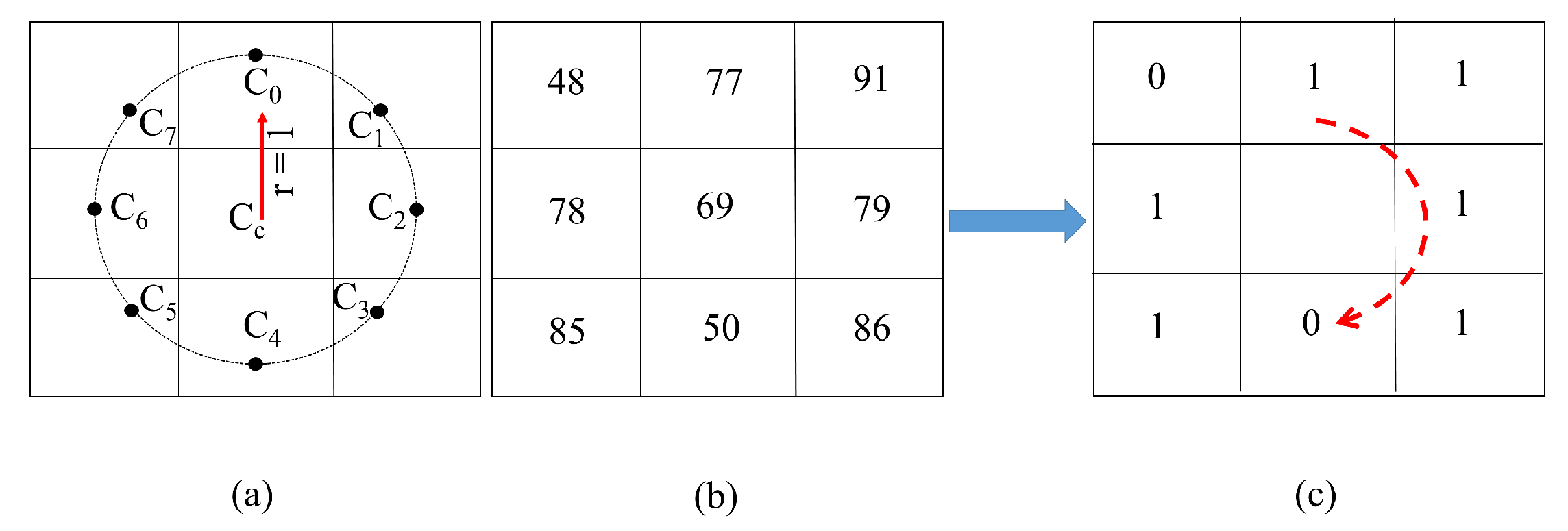
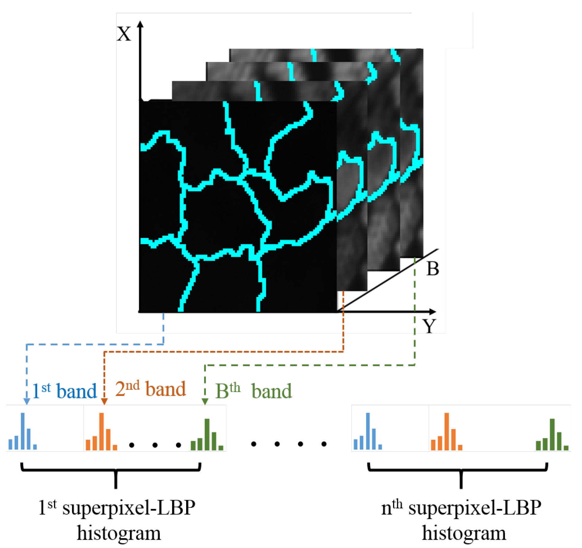
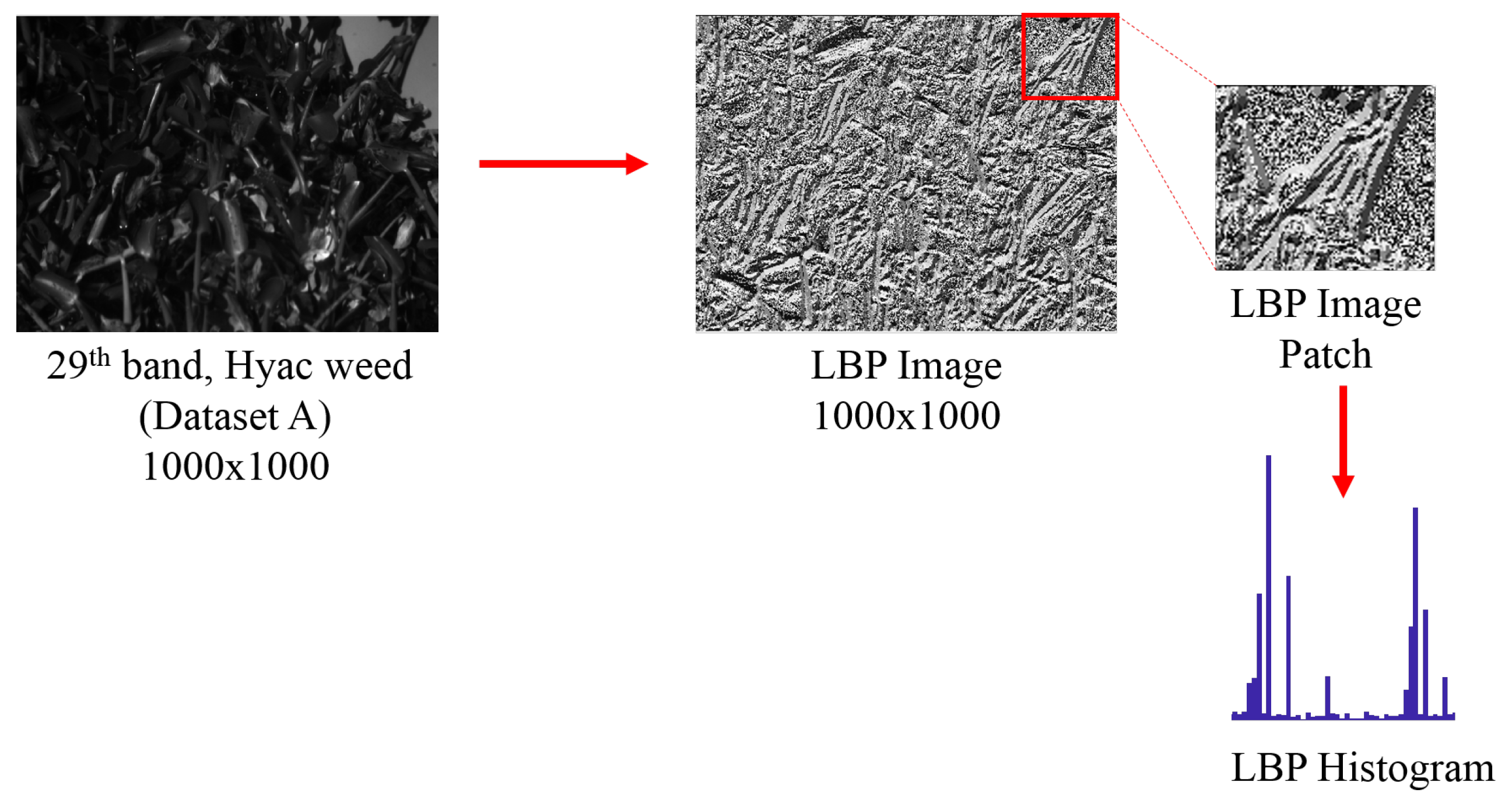
2.2. Superpixel-Based Local Binary Pattern (SPLBP)

LBP is suitable to extract local texture features. To make its spatial properties more effective and descriptive, LBP is applied at superpixel levels. The SLIC based superpixel segmentation method is widely used by the researchers in remote sensing. With this multi-resolution challenge, it is important to utilize a strategy that divides the image into non-uniform regions depending upon the structure of the object. Weeds generally are of different shapes and structures. Therefore, it is important to segment the image based on the structure of the weeds so that in-depth features can be extracted. Superpixels can be generated using SLIC as follows [46]:

• The input image is converted to the CIELAB color space.
• The five-dimensional vector $(l,a,b,x,y)$ is obtained from each pixel, where $(l,a,b)$ are the LAB pixel components and $(x,y)$ are the coordinates of the image pixel.
• To achieve the clustering on a five-dimensional vector, pixel similarity metric is constructed. The similarity metric $D_{ij}$ between pixels $x_i$ and $x_j$ is calculated as follows:

$$D_{lab}=\sqrt{{(l_i-l_j)}^2+{(a_i-a_j)}^2+{(b_i-b_j)}^2},$$

(5)

$$D_{xy}=\sqrt{{(x_i-x_j)}^2+{(y_i-y_j)}^2},$$

(6)

$$D_{ij}=d_{lab}+\frac{M}{S}{d}_{xy},$$

(7)

where each superpixel’s area is represented as S. M is the degree of polymerization. Using the initial cluster (i.e., divide the image into equal parts), the clustering process is continuously updated until it converges using the gradient ascent method. The output of the SLIC based superpixel is a label matrix of each superpixel which is then further used to extract superpixel from each band to form a superpixel cube.

The LBP is obtained for each superpixel as shown in Figure 3. Considering the central pixel $C_p$, the neighbour pixels of central pixel are assigned with a binary label (i.e., ‘0’or ‘1’) depending upon if their values are larger or smaller than the central pixel’s value. Using circular neighborhood of the pixel values, the LBP code of the centre pixel $(x,y)$ can be calculated mathematically as:

$$LB{P}_{(m,r)}\left(C_n\right)=\sum _{i=0}^{m-1}U(C_p-C_n)2^i,$$

(8)

where

$$U(C_p-C_n)=\left\{\begin{array}{c}1,C_p>C_n,\hfill \\ 0,C_p\le C_n,\hfill \end{array}\right.$$

(9)

where $P=m-1$ is the number of sampling points on the circle of the radius r. $C_p$ is the central pixel and $C_n$ is the $n-th$ neighbourhood. Both $C_p$ and $C_n$ have gray value pixels. Figure 3 shows an example of binary thresholding process of eight circular neighbours of the central pixel $C_p$. In the following, the LBP code is computed in the clockwise direction. If the coordinates of the central pixel is $(0,0)$, then each neighbour $C_p$ can be calculated as $rsin(2\pi /m),rcos(2\pi /m)$. The number of sampling point and radius may possess different combinations i.e., (4, 2), (8,3), etc. Bilinear interpolation [37] is used on the locations of the circular neighbours which do not match absolutely on the image mesh. The output of the Equation (8) shows that the binary labels represent the smoothness and texture orientation in the local region. After acquiring the LBP binary labels, the histogram is computed over the local patch. Finally, in order to make the histogram features of equal size, a binning procedure is applied. As each band contains different information, therefore, the LBP operator is then applied on all the bands of superpixels separately. The histogram of each band is also calculated individually and then concatenated to form one feature vector of the superpixel cube. Similarly, the LBP histogram is computed for all the superpixel cubes. The complete process of concatenating SPLBP features is shown in Figure 4.

2.3. Feature Fusion

Feature concatenation is adopted in this study. Each feature set shows different meaning and has its special properties. SPLBP features reflect the local texture of each spatial structure in an image and FCNN extracts different levels of features from low to high. These features, including mid layer features of FCNN, are concatenated into one composite feature vector. Before stacking these feature sets, feature normalization is performed using a linear transformation method. It sets the feature values in the range of [0, 1] with the relationship among the data preserved. After normalization, feature vectors are stacked as $Feat\_vector=\left[Feat\_SPLBP,Feat\_FCNN]\right]$.

2.4. Classification of Fused Features

SVM [47,48] is widely used for remote sensing image classification [21,27]. The motivation for using SVM are: it is a supervised non-parametric statistical learning approach and it works well where a limited amount of data are available [49]. Features extracted using CNN, FCNN, SPLBP and the fused features are classified using the SVM method. Fused features (FCNN-SPLBP) are heterogeneous as they contain both handcrafted and learned features. Consider a training sample with C classes arranged row-wise $x={[x_1,x_2,\dots ,x_C]}^2$, where $x_k(k=1,2,\dots ,C)$ is the subset of training associated with class k. One-versus-one approach is used for the experiments, therefore binary labels $y_i\in \left\{1,-1\right\}$ are used. Binary classes are separated in the kernel-induced space by defining the optimal hyperplane as:

$$mi{n}_{w,\xi ,p}=\left\{\frac{1}{2}{∥\omega ∥}^2+\varsigma \sum _{i=1}^n{\xi }_i\right\},$$

(10)

subject to:

$$y_i\left(〈\varphi (\omega ,x_i)〉\right)+p)\ge 1-{\xi }_i,$$

(11)

where $\varphi$ is the nonlinear kernel mapping that maps the input x into m dimensional vector space, n is the number of samples, p is the bias term, regularization parameter $\varsigma$, ${\xi }_i\ge 0$ for $i=1,\dots ,n$, $\omega$ is the weight, which controls the generalization capacity. ${\xi }_i$ is the non-negative slack variable allows for accommodating errors. The above-mentioned issue is resolved using the Lagrangian dual form.

Radial Based Function (RBF) kernel is used in this paper, and which is represented as:

$$K(x_i,x_j)=exp\left(-\frac{{∥x_i-x_j∥}^2}{2{\sigma }^2}\right),$$

(12)

where the width parameter is $\sigma$ and the decision function is represented as

$$f\left(x\right)=sgn\left(\sum _{i=1}^n{\beta }_i{y}_{i}K(x_i,x)+p\right).$$

(13)

3. Experimental Settings and Results

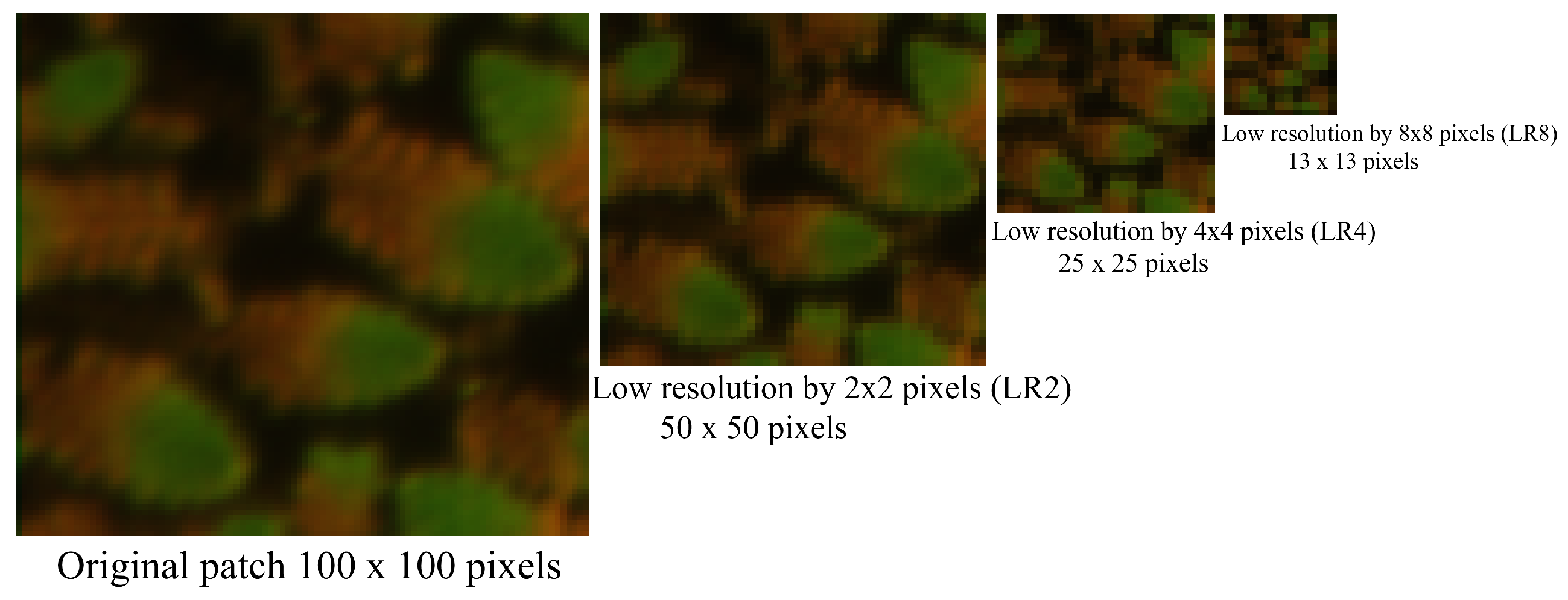
3.1. Hyper/Multi-Spectral Dataset

In this paper, two different weed datasets i.e., UNSW hyperspectral weed dataset (Dataset A) and Multispectral weed dataset (Dataset B) are used for the investigation and validation of the effectiveness and superiority of the proposed architecture. These datasets are described as follows:

(1) Dataset A [12] was captured using a JAI BM-141 camera and a Brimrose VA210 filter with 61 bands which covers the wavelength from 400 nm to 1000 nm. The spatial resolution is $1040\times 1320$ pixels and the spectral resolution of each band is 10 nm by average. This hyperspectral dataset consists of four different categories of weeds which are Alli, Hyme, Hyac, and Azol. Example images of these weeds are demonstrated in Figure 5. As a pre-processing step, each hyperspectral cube in the dataset is cropped from the edges to reduce the image size (i.e., $1000\times 1000$) pixels. As the weed covered the whole image, therefore, the image is divided into 10 equal size patches of $100\times 100$ pixels.

Table 1. Number of hyperspectral cubes in Dataset A.

No	Class	Total_Images
1	Azol	100
2	Alli	200
3	Hyac	100
4	Hyme	200

shows the number of samples in Dataset A. Due to the limited dataset, this size is chosen to generate different hyperspectral cubes of the same category.

(2) The Sequoia multispectral sensor was used to capture Dataset B [2]. This sensor captures four bands (i.e., Green (550 nm), Red (660 nm), Red Edge (735 nm), and NIR (790 nm)). The spatial dimension of each band is $1280\times 960$ pixels. Images are captured at the altitude of 2 m, therefore each multispectral cube consists of multiple weed and crop plants. Hence, from each multispectral image, crops and weeds image patches are randomly selected and then crops are labelled as 0, weed as 1 and mix (weed + crop) as 2. In total, 142 and 198 multispectral cubes are generated for the crop and weed categories, respectively. To make the problem more challenging, there are 188 multispectral images of mixed categories in which weed is mixed with the crop.

Table 2. Number of multispectral cubes from the Dataset B.

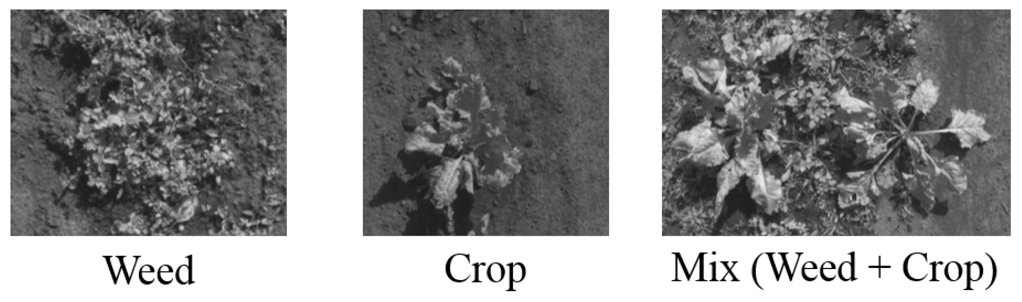
No	Class	Total_Images
1	Crop	142
2	Weed	198
3	Mix (Crop + Weed)	188

shows the number of available samples in Dataset B and Figure 6 shows the sample images of weed, crop and mix.

To demonstrate the multi-resolution problem, images of different resolutions were artificially generated. In this paper, three different resolutions were simulated via the down-sampling method. For example, $LR2$ is computed by averaging $2\times 2$ pixels. The size of the $LR2$ image is half of the input image. In a similar way, the $LR4$ image is averaged by $4\times 4$ and for $LR8$, $8\times 8$ pixels are averaged. Correspondingly, the size of the $LR4$ image is $1/4$ and $LR8$ is $1/8$ of the actual image. Example multi-resolution patches are demonstrated in Figure 7.

The MATLAB based MatConvNet [50] library is utilized for the implementation of the deep CNN method. For the experiments, the number of images in both data sets were artificially increased using data augmentation strategies. Each image is rotated with five different angles. After that, three different images are randomly cropped. The size of the cropped image is 90–95% of the original image. The size of the input image to all the algorithms used in this study was set to $56\times 56$. The dataset is randomly divided into three sets i.e., training set (60%), testing set (20%) and validation set (20%). Data augmentation is only applied to images in the training set. To make the comparison reliable, each experiment was repeated 10 times with different, randomly split training, testing and validation sets. Feature extraction and learning method(s) such as CNN, FCNN, LBP, superpixel based LBP, and FCNN-superpixel based LBP methods were compared. The overall accuracy (OA) was used to assess the classification performance. For CNN, convolutional layers CONV1, CONV2, CONV3 and CONV4 with pad size 1 were implemented. For the pooling layer, kernel size was [2, 2] and stride was 2. To avoid over-fitting, two dropout layers (i.e., DPO1 and DPO2) were introduced of ratio 0.5. Finally, fully connected (FC) layers are added at the top of all the layers followed by the softmax loss function for the training of the model. The value of batch size is set to 100. The learning rate is set to ${10}^{-5}$ for Dataset A and ${10}^{-3}$ for Dataset B. The optimizer used in this work is SGD with momentum. The number of iterations is set to 100 for Dataset A and 50 for Dataset B.

LBP features are computed from each band using the build-in MATLAB function. Figure 3 shows the implementation of the LBP feature extraction. Parameters of LBP such as $(m,r)$ play an important role in the classification process, where r is the radius that determines the region for selecting circular neighbours and m defines the dimensionality of the LBP histogram. For HSI or Multispectral dataset R$\in R^{X\times Y\times B}$, where B is the number of bands, each band is used as a gray-scale image to extract the LBP feature. Figure 8 displays LBP texture feature extraction of the 29th band of the Hyac weed category from Dataset A. After feature extraction from each band, all the features are concatenated to get the final LBP feature vector.

Table 3. Classification accuracy of the Local Binary Pattern (LBP) method with parameter values $(m,r)$ using Dataset A.

m	4	6	8	10
$r=1$	$72.85$	$73.42$	$75.63$	$75.22$
$r=2$	$73.65$	$74.19$	$\mathbf{76.75}$	$75.55$
$r=3$	$71.32$	$72.85$	$74.38$	$73.89$

shows the classification accuracies of LBP method using different $(m,r)$ values on Dataset A. The results show that the accuracy is steady when $(m\ge 8)$ and is insensitive to the value of r. Based on the classification accuracies in Table 3, the optimal values are $m=8$ and $r=2$. Similarly, the SLIC algorithm is used to generate $n=9$ superpixels from each band.

3.2. Classification Results and Discussions

Table 4. Mean and overall accuracy (%) using CNN, LBP, FCNN, SPLBP and FCNN-SPLBP for Dataset A.

Class	CNN Mean Accuracy	LBP Mean Accuracy	FCNN Mean Accuracy	SPLBP Mean Accuracy	FCNN-SPLBP Mean Accuracy
1	$78.40$	$83.64$	$92.55$	$82.75$	$\mathbf{92.80}$
2	$76.65$	$72.45$	$82.85$	$76.82$	$\mathbf{91.47}$
3	$74.89$	$65.45$	$78.25$	$79.26$	$\mathbf{89.55}$
4	$73.3$	$67.80$	$70.35$	$71.48$	$\mathbf{88.62}$
OA	$79.3\pm 0.22$	$75.8\pm 0.30$	$85.7\pm 0.18$	$80.25\pm 0.25$	$89.70\pm 0.35$

and

Table 5. Mean and overall accuracy (%) using CNN, LBP, FCNN, SPLBP and FCNN-SPLBP for Dataset B.

Class	CNN Mean Accuracy	LBP Mean Accuracy	FCNN Mean Accuracy	SPLBP Mean Accuracy	FCNN-SPLBP Mean Accuracy
1	$91.78$	$81.56$	$93.63$	$94.21$	$\mathbf{95.84}$
2	$94.73$	$82.28$	$94.82$	$95.55$	$\mathbf{96.7}$
3	$80.6$	$77.96$	$83.28$	$83.78$	$\mathbf{88.45}$
OA	$89.75\pm 0.74$	$83.64\pm 0.90$	$92.5\pm 0.55$	$91.67\pm 0.65$	$96.35\pm 0.77$

show the OA using CNN, FCNN, LBP, SPLBP and FCNN-SPLBP on Dataset A and Dataset B. From Table 4 and Table 5, it can be seen that the performance of FCNN, SPLBP, FCNN-SPLBP methods increases when texture, mid and high-level features are added.

3.2.1. Dataset A

The multi-resolution problem is itself a challenging problem to deal with. Table 4 shows the mean accuracy of each class and the OA of different algorithms such as CNN, FCNN, LBP, SPLBP and FCNN-SPLBP. From the results on the CNN method, it can be seen that, for the multi-resolution Dataset A, the features extracted from the higher layers cannot clearly distinguish each category of weed. Usually, CNN is designed for one standard resolution of images to get valuable features at higher layers. However, from the results in Table 4, it is observed that traditional CNN-based stacked layer feature extraction method is not suitable for the multi-resolution images.

FCNN architecture fuses features from different layers for multi-resolution images. As shown in [42,43], each layer of the traditional CNN architecture provides different level of features. For instance, at earlier layers, low-level features can be extracted such as edges and blobs. At mid-layers, more discriminative features can be extracted. These mid-level features are useful to deal with the low-resolution images. This phenomenon is proved with the experimental results. As shown in Table 4, the overall accuracy for the FCNN architecture is improved by 6.4% by adding additional information (i.e., mid-level features) with high-level features when these features are concatenated and classified using the SVM classifier.

Local texture features are compared with feature learning method in their classification performance. Results in Table 4 show that they achieve low recognition accuracy as compared to the CNN and FCNN methods. These local features are hand-crafted which are only designed to resolve specific issues. These texture features are not generalized enough for the classification of multi-resolution images. Therefore, it is difficult to distinguish each category and overall recognition accuracy is low as compared to CNN and FCNN.

To address this issue, a method based on superpixel and LBP (SPLBP) is proposed. This method uses a superpixel to extract clear object boundaries of each weed category within the image and then local texture features are obtained from each superpixel. These dense local features are then used with the SVM classifier for the classification. Results on Dataset A show improvement as compared to the local features extracted from the entire image. The combination of SPLBP features shows significant improvement in Table 4 compared to the LBP method. Moreover, equivalent results are achieved with CNN and FCNN.

To achieve high recognition accuracy for the multi-resolution dataset, it is found that additional information in a feature representation is required. Therefore, a combination of dense local texture and fusion of features from mid and high layers of CNN are concatenated to form a rich feature representation. This dense feature representation shows significant improvement in Table 4. Finally, it is observed that utilizing rich information from different layers of a feature learning method, it is possible to achieve an improved recognition accuracy by 5.45%.

Overall, the experiments are repeated 10 times to analyze the robustness of the proposed method. From the repetition, it is found that there is a variation of about ± 0.35% in the overall accuracy of the FCNN-SPLBP method. This shows that the proposed feature extraction and combination of features are generalized enough to deal with the variations in the training and testing sets.

3.2.2. Dataset B

Similarly, there are three classes i.e., crop, weed and mix (crop + weed) in Dataset B. Using the CNN architecture, multi-resolution images in Dataset B were evaluated, whose results are shown in Table 5. High-level features extracted from the final layer were not discriminative enough to deal with the multi-resolution images. Therefore, we needed to have a feature vector that can deal with both high-resolution and low-resolution images at the same time.

To address this issue, the FCNN model is trained and tested using SVM. This model exploits the features extracted from the mid and high-layers. From the results in Table 5, it is found that the combination of mid-level and high-level features are more discriminative and robust as compared to the traditional CNN architecture. As a result, the overall accuracy is increased by 2.75 percent for the test data.

The feature learning method is then compared to handcrafted feature extraction method. Using LBP, the overall accuracy is decreased by 6.11% as compared to the CNN methods and 8.86% compared to the FCNN, respectively. From these facts, it is observed that the local features alone are not suitable to deal with the multi-resolution weed dataset as they are not designed for these scenarios. By dividing the image using the structural information of the weeds, superpixels are used with the LBP (i.e., SPLBP) to deal with the multi-resolution images. Using the SPLBP method, the testing accuracy is improved as compared to the LBP method on Dataset B. From the results in Table 5, it is observed that the accuracy of SPLBP is comparable to CNN and FCNN. Therefore, investigating the combination of local, mid-level and high-level features for the multi-resolution data are worthwhile.

A combination of local (i.e., SPLBP), mid-level and high-level features from FCNN architecture is trained and tested using the SVM classifier. Table 5 shows the mean accuracy of each class and overall accuracy achieved using FCNN-SPLBP. Results indicate that it is possible to deal with the multi-resolution issues of the weed classification using the combination of feature levels. Overall, the performance of superpixels based methods (SPLBP and FCNN-SPLBP) is higher as compared to the non-superpixel based methods (CNN, FCNN, LBP). This indicates the importance of using superpixels for the classification of weed categories. Our proposed FCNN-SPLBP method consistently shows the best results, which delivers significant improvements of the classification performance over the compared methods on Dataset B.

Hence, it is established that to handle the multi-resolution weed classification problem there is a need for complete feature representation to correctly classify each category of weed. As each sensor captures the data with it’s own specification, this feature representation method will help to address this issue.

Similar to the setting for Dataset A, the experiment on Dataset B is done 10 times for FCNN-SPLBP. For each experiment, the training (60%), validation (20%) and testing (20%) are sampled randomly. The total variation observed on the overall accuracy is ± 0.77%.

4. Conclusions

In this paper, we propose a framework FCNN-SPLBP that utilizes several levels of features for the classification of weeds in remote sensing images. The proposed framework uses high-level and mid-level features from a CNN-based feature learning method and extracts low-level features using the SP based LBP coding. This novel framework greatly increases the overall performance of the system particularly when dealing with the multi-resolution data. The experiments demonstrate the superiority of the FCNN-SPLBP method over CNN, LBP, and SPLBP on two remote sensing datasets. Given the increasingly available multisensor datasets, the proposed framework would be advantageous in this area and offer great value for multi-resolution image classification.

References

- Invasive Plants and Animals Committee. Australian Weeds Strategy 2017 to 2027; Australian Government Department of Agriculture of Water Resources: Canberra, Australia, 2016.
- Sa, I.; Chen, Z.; Popovi, M.; Khanna, R.; Liebisch, F.; Nieto, J.; Siegwart, R. WeedNet: Dense semantic weed classification using multispectral images and MAV for smart farming. IEEE Robot. Autom. Lett. 2018, 3, 588–595. [Google Scholar] [CrossRef]
- Pearlstein, L.; Kim, M.; Seto, W. Convolutional neural network application to plant detection, based on synthetic imagery. In Proceedings of the 2016 IEEE Applied Imagery Pattern Recognition Workshop (AIPR), Washington, DC, USA, 18–20 October 2016; pp. 1–4. [Google Scholar]
- Hung, C.; Xu, Z.; Sukkarieh, S. Feature learning based approach for weed classification using high-resolution aerial images from a digital camera mounted on a UAV. Remote Sens. 2014, 6, 12037–12054. [Google Scholar] [CrossRef]
- Paoletti, M.; Haut, J.; Plaza, J.; Plaza, A. A new deep convolutional neural network for fast hyperspectral image classification. ISPRS J. Photogramm. Remote Sens. 2018, 145, 120–147. [Google Scholar] [CrossRef]
- Chavan, T.R.; Nandedkar, A.V. Agroavnet for crops and weeds classification: A step forward in automatic farming. Comput. Electron. Agric. 2018, 154, 361–372. [Google Scholar] [CrossRef]
- Burks, T.; Shearer, S.; Gates, R.; Donohue, K. Backpropagation neural network design and evaluation for classifying weed species using color image texture. Trans. ASAE 2000, 43, 1029. [Google Scholar] [CrossRef]
- Burks, T.; Shearer, S.; Payne, F. Classification of weed species using color texture features and discriminant analysis. Trans. ASAE 2000, 43, 1001. [Google Scholar] [CrossRef]
- El-Faki, M.; Zhang, N.; Peterson, D. Factors affecting color-based weed detection. Trans. ASAE 2000, 43, 441. [Google Scholar]
- Guo, W.; Rage, U.K.; Ninomiya, S. Illumination invariant segmentation of vegetation for time series wheat images based on decision tree model. Comput. Electron. Agric. 2013, 96, 58–66. [Google Scholar] [CrossRef]
- Perez-Ortiz, M.; Pena, J.M.; Gutierrez, P.A.; Torres-Sanchez, J.; Hervas-Martnez, C.; Lopez-Granados, F. Selecting patterns and features for between-and within-crop-row weed mapping using uav imagery. Expert Syst. Appl. 2016, 47, 85–94. [Google Scholar] [CrossRef]
- Farooq, A.; Hu, J.; Jia, X. Analysis of spectral bands and spatial resolutions for weed classification via deep convolutional neural network. IEEE Geosci. Remote. Sens. Lett. 2018, 16, 183–187. [Google Scholar] [CrossRef]
- Ojala, T.; Pietikainen, M.; Maenpaa, T. Multiresolution gray-scale and rotation invariant texture classification with local binary patterns. IEEE Trans. Pattern Anal. Mach. Intell. 2002, 24, 971–987. [Google Scholar] [CrossRef]
- Brahnam, S.; Jain, L.C.; Nanni, L.; Lumini, A. Local Binary Patterns: New Variants and Applications; Springer: Berlin/Heidelberg, Germany, 2014. [Google Scholar]
- Zhao, G.; Pietikainen, M. Dynamic texture recognition using local binary patterns with an application to facial expressions. IEEE Trans. Pattern Anal. Mach. Intell. 2007, 29, 915–928. [Google Scholar] [CrossRef] [PubMed]
- Guo, Z.; Wang, X.; Zhou, J.; You, J. Robust texture image representation by scale selective local binary patterns. IEEE Trans. Image Process. 2016, 25, 687–699. [Google Scholar] [CrossRef] [PubMed]
- Liao, S.; Law, M.W.; Chung, A.C. Dominant local binary patterns for texture classification. IEEE Trans. Image Process. 2009, 18, 1107–1118. [Google Scholar] [CrossRef] [PubMed]
- Guo, Z.; Zhang, L.; Zhang, D. Rotation invariant texture classification using lbp variance (lbpv) with global matching. Pattern Recognit. 2010, 43, 706–719. [Google Scholar] [CrossRef]
- Pietikainen, M.; Ojala, T.; Xu, Z. Rotation-invariant texture classification using feature distributions. Pattern Recognit. 2000, 33, 43–52. [Google Scholar] [CrossRef] [Green Version]
- Musci, M.; Feitosa, R.Q.; da Costa, G.A.O.P.; Velloso, M.L.F. Assessment of binary coding techniques for texture characterization in remote sensing imagery. IEEE Geosci. Remote Sens. Lett. 2013, 10, 1607–1611. [Google Scholar] [CrossRef]
- Li, W.; Chen, C.; Su, H.; Du, Q. Local binary patterns and extreme learning machine for hyperspectral imagery classification. IEEE Trans. Geosci. Remote. Sens. 2015, 53, 3681–3693. [Google Scholar] [CrossRef]
- Liu, M.-Y.; Tuzel, O.; Ramalingam, S.; Chellappa, R. Entropy rate superpixel segmentation. In Proceedings of the IEEE Conference on Computer Vision and Pattern Recognition (CVPR), Washington, DC, USA, 20–25 June 2011; pp. 2097–2104. [Google Scholar]
- Shi, J.; Malik, J. Normalized cuts and image segmentation. IEEE Trans. Pattern Anal. Mach. Intell. 2000, 22, 888–905. [Google Scholar]
- Achanta, R.; Shaji, A.; Smith, K.; Lucchi, A.; Fua, P.; Susstrunk, S. Slic superpixels compared to state-of-the-art superpixel methods. IEEE Trans. Pattern Anal. Mach. Intell. 2012, 34, 2274–2282. [Google Scholar] [CrossRef]
- Fang, L.; Li, S.; Duan, W.; Ren, J.; Benediktsson, J.A. Classification of hyperspectral images by exploiting spectralspatial information of superpixel via multiple kernels. IEEE Trans. Geosci. Remote Sens. 2015, 53, 6663–6674. [Google Scholar] [CrossRef]
- Li, J.; Zhang, H.; Zhang, L. Efficient superpixel-level multitask joint sparse representation for hyperspectral image classification. IEEE Trans. Geosci. Remote Sens. 2015, 53, 5338–5351. [Google Scholar]
- Jia, S.; Deng, B.; Zhu, J.; Jia, X.; Li, Q. Local binary pattern-based hyperspectral image classification with superpixel guidance. IEEE Trans. Geosci. Remote. Sens. 2018, 56, 749–759. [Google Scholar] [CrossRef]
- Chen, Z.; Wang, B. An improved spectral-spatial classification framework for hyperspectral remote sensing images. In Proceedings of the International Conference on Audio, Language and Image Processing (ICALIP), Shanghai, China, 7–9 July 2014; pp. 532–536. [Google Scholar]
- He, Z.; Shen, Y.; Zhang, M.; Wang, Q.; Wang, Y.; Yu, R. Spectralspatial hyperspectral image classification via svm and superpixel segmentation. In Proceedings of the International Proceedings on Instrumentation and Measurement Technology Conference (I2MTC), Montevideo, Uruguay, 12–15 May 2014; pp. 422–427. [Google Scholar]
- Lottes, P.; Horferlin, M.; Sander, S.; Stachniss, C. Effective vision based classification for separating sugar beets and weeds for precision farming. J. Field Robot. 2017, 34, 1160–1178. [Google Scholar] [CrossRef]
- Lottes, P.; Khanna, R.; Pfeifer, J.; Siegwart, R.; Stachniss, C. UAV based crop and weed classification for smart farming. In Proceedings of the IEEE International Conference on Robotics and Automation (ICRA), Singapore, 29 May–3 June 2017; pp. 3024–3031. [Google Scholar]
- McCool, C.; Perez, T.; Upcroft, B. Mixtures of lightweight deep convolutional neural networks: applied to agricultural robotics. IEEE Robot. Autom. Lett. 2017, 2, 1344–1351. [Google Scholar] [CrossRef]
- Milioto, A.; Lottes, P.; Stachniss, C. Real-time semantic segmentation of crop and weed for precision agriculture robots leveraging background knowledge in CNNs. In Proceedings of the IEEE International Conference on Robotics and Automation (ICRA), Brisbane, Australia, 21–26 May 2018; pp. 2229–2235. [Google Scholar]
- Sellami, A.; Farah, M.; Farah, I.R.; Solaiman, B. Hyperspectral imagery classification based on semi-supervised 3D deep neural network and adaptive band selection. Expert Syst. Appl. 2019, 129, 246–259. [Google Scholar] [CrossRef]
- Li, Y.; Zhang, H.; Shen, Q. Spectral–spatial classification of hyperspectral imagery with 3D convolutional neural network. Remote Sens. 2017, 9, 67. [Google Scholar] [CrossRef]
- Mortensen, A.K.; Dyrmann, M.; Karstoft, H.; Jorgensen, R.N.; Gislum, R. Semantic segmentation of mixed crops using deep convolutional neural network. In Proceedings of the International Conference on Agricultural Engineering, Aarhus, Denmark, 28–29 June 2016. [Google Scholar]
- Potena, C.; Nardi, D.; Pretto, A. Fast and accurate crop and weed identification with summarized train sets for precision agriculture. In Proceedings of the International Conference on Intelligent Autonomous Systems, Shanghai, China, 3–7 July 2016; pp. 105–121. [Google Scholar]
- dos Santos Ferreira, A.; Freitas, D.M.; da Silva, G.G.; Pistori, H.; Folhes, M.T. Weed detection in soybean crops using convnets. Comput. Electron. Agric. 2017, 143, 314–324. [Google Scholar] [CrossRef]
- Zhang, L.; Zhang, L.; Du, B. Deep learning for remote sensing data: A technical tutorial on the state of the art. IEEE Geosci. Remote. Sens. Mag. 2016, 4, 22–40. [Google Scholar] [CrossRef]
- Rumelhart, D.E.; Hinton, G.E.; Williams, R.J. Learning representations by back-propagating errors. Nature 1986, 323, 533. [Google Scholar] [CrossRef]
- Wilson, A.C.; Roelofs, R.; Stern, M.; Srebro, N.; Recht, B. The marginal value of adaptive gradient methods in machine learning. In Advances in Neural Information Processing Systems; The MIT Press: Cambridge, MA, USA, 2017; pp. 4148–4158. [Google Scholar]
- Zeiler, M.D.; Fergus, R. Visualizing and understanding convolutional networks. In Proceedings of the European Conference on Computer Vision, Zurich, Switzerland, 6–12 September 2014; pp. 818–833. [Google Scholar]
- Lee, S.H.; Chan, C.S.; Mayo, S.J.; Remagnino, P. How deep learning extracts and learns leaf features for plant classification. Pattern Recognit. 2017, 71, 1–13. [Google Scholar] [CrossRef] [Green Version]
- Chen, Z.; Lam, O.; Jacobson, A.; Milford, M. Convolutional neural network-based place recognition. arXiv 2014, arXiv:1411.1509. [Google Scholar]
- Oquab, M.; Bottou, L.; Laptev, I.; Sivic, J. Learning and transferring mid-level image representations using convolutional neural networks. In Proceedings of the IEEE Conference on Computer Vision and Pattern Recognition (CVPR), Columbus, OH, USA, 24–27 June 2014; pp. 1717–1724. [Google Scholar]
- Sun, X.; Zhang, F.; Yang, L.; Zhang, B.; Gao, L. A hyperspectral image spectral unmixing method integrating slic superpixel segmentation. In Proceedings of the 7th Workshop on Hyperspectral Image and Signal Processing: Evolution in Remote Sensing (WHISPERS), Tokyo, Japan, 2–5 June 2015; pp. 1–4. [Google Scholar]
- Li, W.; Prasad, S.; Fowler, J.E.; Bruce, L.M. Locality-preserving dimensionality reduction and classification for hyperspectral image analysis. IEEE Trans. Geosci. Remote Sens. 2012, 50, 1185–1198. [Google Scholar] [CrossRef]
- Camps-Valls, G.; Gomez-Chova, L.; Munoz-Mari, J.; Vila-Frances, J.; Calpe-Maravilla, J. Composite kernels for hyperspectral image classification. IEEE Geosci. Remote Sens. Lett. 2014, 3, 93–97. [Google Scholar] [CrossRef]
- Mountrakis, G.; Im, J.; Ogole, C. Support vector machines in remote sensing: A review. ISPRS J. Photogramm. Remote Sens. 2011, 66, 247–259. [Google Scholar] [CrossRef]
- Vedaldi, A.; Lenc, K. Matconvnet: Convolutional neural networks for matlab. In Proceedings of the 23rd ACM International Conference on Multimedia, Brisbane, Australia, 26–30 October 2015; pp. 689–692. [Google Scholar]