Wind Speed Retrieval from Simulated RADARSAT Constellation Mission Compact Polarimetry SAR Data for Marine Application

Abstract

RADARSAT Constellation Mission (RCM) compact polarimetry (CP) data were simulated using 504 RADARSAT-2 quad-pol SAR images. These images were used to samples CP data in three RCM modes to build a data set with co-located ocean wind vector observations from in situ buoys on the West and East coasts of Canada. Wind speeds up to 18 m/s were included. CP and linear polarization parameters were related to the C-band model (CMOD) geophysical model functions CMOD-IFR2 and CMOD5n. These were evaluated for their wind retrieval potential in each RCM mode. The CP parameter Conformity was investigated to establish a data-quality threshold (>0.2), to ensure high-quality data for model validation. An accuracy analysis shows that the first Stokes vector (SV₀) and the right-transmit vertical-receive backscatter (RV) parameters were as good as the VV backscatter with CMOD inversion. SV₀ produced wind speed retrieval accuracies between 2.13 m/s and 2.22 m/s, depending on the RCM mode. The RCM Medium Resolution 50 m mode produced the best results. The Low Resolution 100 m and Low Noise modes provided similar results. The efficacy of SV₀ and RV imparts confidence in the continuity of robust wind speed retrieval with RCM CP data. Three image-based case studies illustrate the potential for the application of CP parameters and RCM modes in operational wind retrieval systems. The results of this study provide guidance to direct research objectives once RCM is launched. The results also provide guidance for operational RCM data implementation in Canada’s National SAR winds system, which provides near-real-time wind speed estimates to operational marine forecasters and meteorologists within Environment and Climate Change Canada.

1. Introduction

Wind speed retrieval using spaceborne scatterometer and synthetic aperture radar (SAR) data is a mature field with operational implementation in many countries. The most widely-used algorithms are the C-band model (CMOD) family of geophysical model functions. These models were based on the relationship of the C-band vertical-transmit vertical-receive (VV) backscatter with wind speed, wind direction and incidence angle, derived from scatterometer data [1,2]. Early development based on European Remote Sensing (ERS-1) scatterometer data resulted in CMOD-IFR2 [1], with additional development producing CMOD4 and CMOD5, to arrive at CMOD5n [2] and, most recently, CMOD7 [3]. SAR imagery applications have employed the CMOD family of models and have also developed SAR-specific models to take advantage of other polarizations. The horizontal-transmit horizontal-receive (HH) SAR backscatter was associated with the CMOD VV backscatter through the use of a polarization ratio (PR) [4,5]. The cross-polarized backscatter, i.e., horizontal-transmit vertical-receive (HV), was associated with wind speed, without wind direction or incidence angle input [5]. Models employing both co- and cross-polarized parameters (i.e., VV and VH), in addition to incidence angle and sensor noise, with or without wind direction, were associated with wind speed and are found to be comparable to or better than CMOD-IFR2 retrievals [6]. Using cross-polarized wind speed retrieval in concert with CMOD5n, [7] reported capabilities for SAR wind direction retrieval. Alternatively, azimuthal smearing due to surface motion was associated with wind speed via the SAR azimuth cutoff [8]. Geophysical model functions relating the azimuth cutoff to wind speed and significant wave height were described by [9]. The azimuth cutoff was explored further by [10], who also establish criteria for the optimal use of azimuth cutoff for wind speed retrieval.

The development of the RADARSAT Constellation Mission (RCM) and Radar Imaging Satellite-1 (RISAT-1) necessitates an examination of C-band compact polarimetry (CP) SAR data for wind retrieval. CP data provides near-polarimetric SAR capabilities, but at much larger swath widths, making these data more operationally viable. However, while RCM and RISAT-1 can provide linear polarizations, in CP mode, no linear polarizations are available, relying instead on right-circular-transmit orthogonal-linear-receive architecture (CTLR) [11,12,13]. Operational systems, such as Canada’s National SAR Winds programme (NSW), must therefore be able to accommodate CP data in their workflows. The CTLR architecture enables the derivation of many CP parameters, several of which are analogous to linear parameters (i.e., right-circular-transmit linear-receive: RV, RH), while others are analogous to polarimetric parameters (e.g., RV-RH phase difference), and still others are a function of the right- or left-circular-return (i.e., RR, RL).

CP data can be simulated from polarimetric data under the assumption of cross-polarized reciprocity. An RCM data simulator, developed by F. Charbonneau at the Canada Centre for Mapping and Earth Observation, Natural Resources Canada, was employed by the authors to simulate the CP data from RADARSAT-2 quad-polarized data [14,15,16,17]. The RCM simulator adds noise to the RADARSAT-2 data to simulate the various RCM mode noise floors. In early versions of the RCM simulator (v.2 in 2013/2014), random noise was added to the first Stokes vector, causing the noise to be cancelled out in the other Stokes vectors [14]. Therefore, noise effects on phase-related parameters could not be assessed. In later versions of the RCM simulator (v.3.1. in 2016), noise was added to the complex imagery prior to Stokes vector generation, allowing phase-related parameters to be evaluated for different noise floors.

A subset of CP parameters can be directly related to CMOD models for wind speed retrieval: these are RV, RH, RL and SV₀ [14,15]. Model functions for RV and RH have also been derived directly from CP data, using both empirical [16] and semi-empirical models associated with Bragg and non-Bragg scattering [17]. Model functions for CP parameters unrelated to CMOD have been derived and have skill in wind speed retrieval; in particular RR [14,18], m-χ-volume [14], and randomly polarized power [15].

Limitations to wind speed retrieval using both CMOD-related parameters and CP parameters are associated with the sensor noise floor and/or the geophysical conditions of the water surface. The higher the noise floor, the more the parameters are affected, particularly those that rely on non-Bragg scattering, i.e., cross-polarized parameters [6,15]. In low wind conditions [19], or in the presence of ocean slicks [20], CP parameters that rely on phase information may also be affected. A low wind speed threshold of 3 m/s is occasionally used to avoid data issues at low wind speeds [17]. Modification to CP parameter values may also originate from rain, internal waves, or ocean currents [17]. Sensor noise and surface conditions can, therefore, lead to poor data quality, which must be considered both during model development and during wind speed retrieval.

In this study, we evaluated the set of CMOD-related CP (CMOD-CP) parameters for their utility in SAR wind speed retrieval. Using a recent version of the RCM simulator (v.3.1.), we aimed to (1) establish a novel data-quality threshold based on CP parameters and (2) test CMOD-CP parameter wind speed retrievals against buoy-observed wind speeds. The latter represents the most robust testing thus far for the full set of CMOD-CP parameters (RV, RH, RL and SV₀), and provides a comparative analysis of two CMOD models (CMOD-IFR2 and CMOD5n) and three RCM modes. We also performed a model comparison between CP and linear CMOD-related parameters. We concluded with a forward look at future data products derived from RCM CP and linear data.

2. Methods

2.1. Data

2.1.1. C-band SAR Data

RCM data were simulated from RADARSAT-2 Fine Quad (FQ) data using the RCM simulator (v.3.1). A total of 504 FQ SAR images were acquired for the period 2008 to 2012, over Environment and Climate Change Canada (ECCC) meteorological buoys. Three RCM modes were simulated: Low Resolution (LowRes), Low Noise (LowNoise) and Medium Resolution (MR50). The specifications of the selected beam modes are shown in

Table 1. Specification of RCM modes used for this study; all modes are capable of providing HH, VV, HH+HV, VV+VH and CP polarizations. LowRes and MR50 are also capable of providing HH+VV [21].

RCM Mode	Short Form	Resolution (m)	Looks (Range × Azimuth)	Swath Width (km) (Accessible)	Nominal NESZ (dB)
Low Resolution (100 m)	LowRes	100	8 × 1	500 (500)	−22
Low Noise	LowNoise	100	4 × 2	350 (600)	−25
Medium Resolution (50 m)	MR50	50	4 × 1	350 (600)	−22

. The simulation options are specification noise floor (NESZ) and speckle filtering using a Sigma-Lee filter with a window size of 7 × 7 and a target size of 5 × 5; no second filter run was used. Backscatter values were in sigma-naught (σ⁰).

Post-simulation image processing included the derivation of additional CP parameters and image georectification. Twenty CP parameters and five linear polarization parameters were used in this study (

Table 2. Compact-polarimetry and linear polarization parameters used in this study.

Short Form	Description
σ0RV,σ0RH, σ0RL	Right-circular transmit, vertical, horizontal, left receive
δRVRH	Phase difference [12]
Conformity	Conformity coefficient [22]
SV0	First Stokes vectors
σ0VV, σ0HH	Linear polarizations

). Image sampling was performed using a 3 × 3 km region of interest (ROI), centred on a meteorological buoy. The mean and standard deviation for each parameter were calculated for each ROI, for each RCM mode simulated. Therefore, the data set comprised 1512 samples (504 × 3 modes). Sample ROIs encompassed ~1915 pixels for the LowNoise and LowRes modes, and ~7680 pixels for the MR50 mode. Parameter values were normalized to decibels (dB) when appropriate for more reliable calculation of the statistics.

2.1.2. Meteorological Data

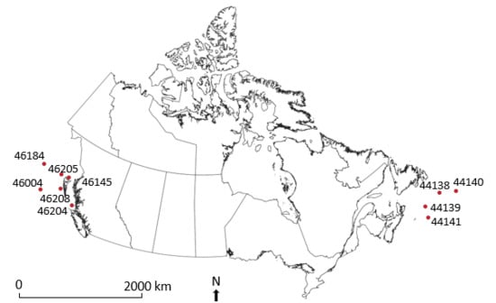
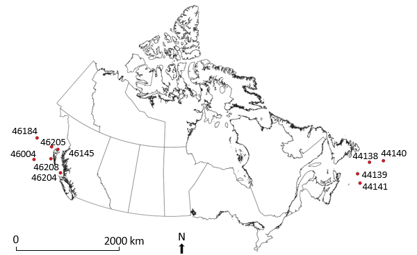
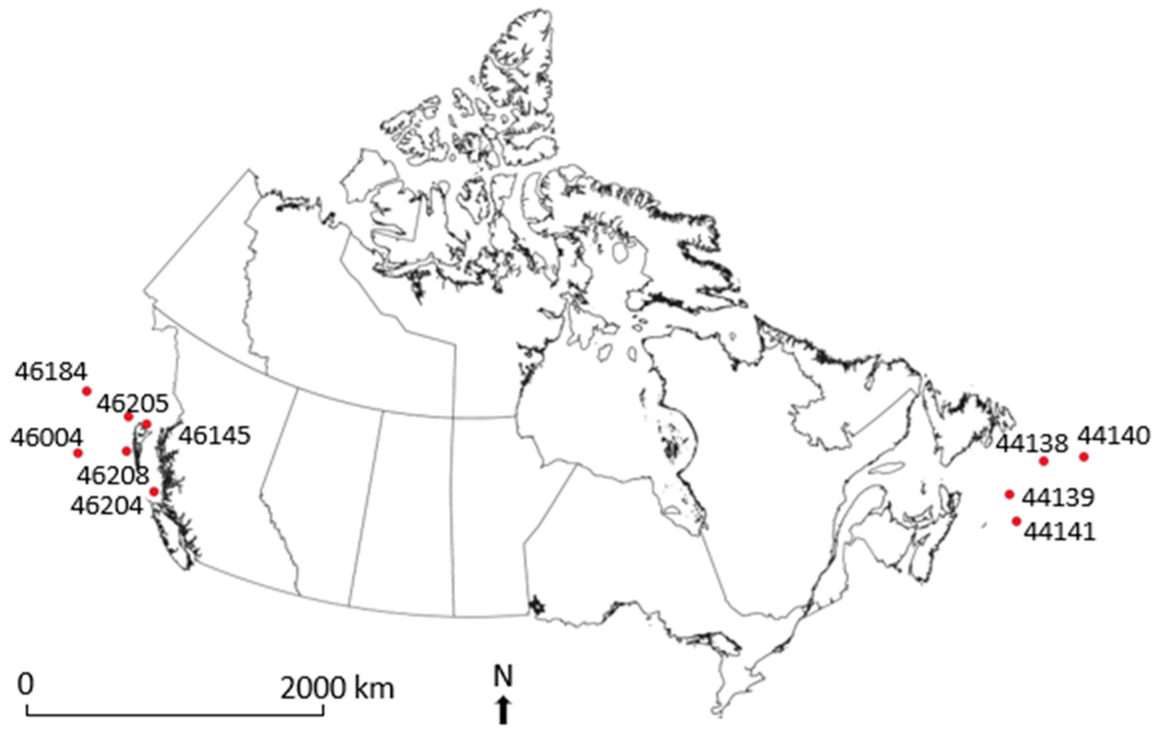
The ECCC meteorological buoys used in this study are in marine areas on the East and West coasts of Canada (Figure 1); these areas have calibrated and well-maintained buoys. The buoys report hourly wind speed and wind direction measured by two sensors, averaged over an eight-minute interval. The observed wind speed was converted to winds at a 10 m reference height above the ocean surface using the Tropical Ocean and Global Atmosphere Coupled Ocean-Atmosphere Response Experiment (TOGA COARE) bulk flux algorithm [23]. Wind direction must be relative to the satellite look direction. This was calculated by adjusting the observed wind direction relative to the satellite track direction +90° (right-looking).

2.2. SAR Data Quality

Various factors can influence the quality of the data used for algorithm development and testing. Spatio-temporal issues concern the temporal, and thus spatial, difference between buoy data at its reporting time and at the SAR acquisition time. These issues were mitigated somewhat by the use of 3 × 3 km ROIs. Two additional factors were spatial variability within sample ROIs, and low-quality backscatter in the proximity of the noise floor.

2.2.1. Spatial Variability

ROIs that exhibit high variability in backscatter are likely representative of image areas (i.e., 3 × 3 km) containing discontinuous wind slicks or strong wind gradients. Such ROI sample values are probably unrepresentative of the buoy wind speed and/or direction. Therefore, they are likely to introduce a significant source of error and should be removed from further analysis.

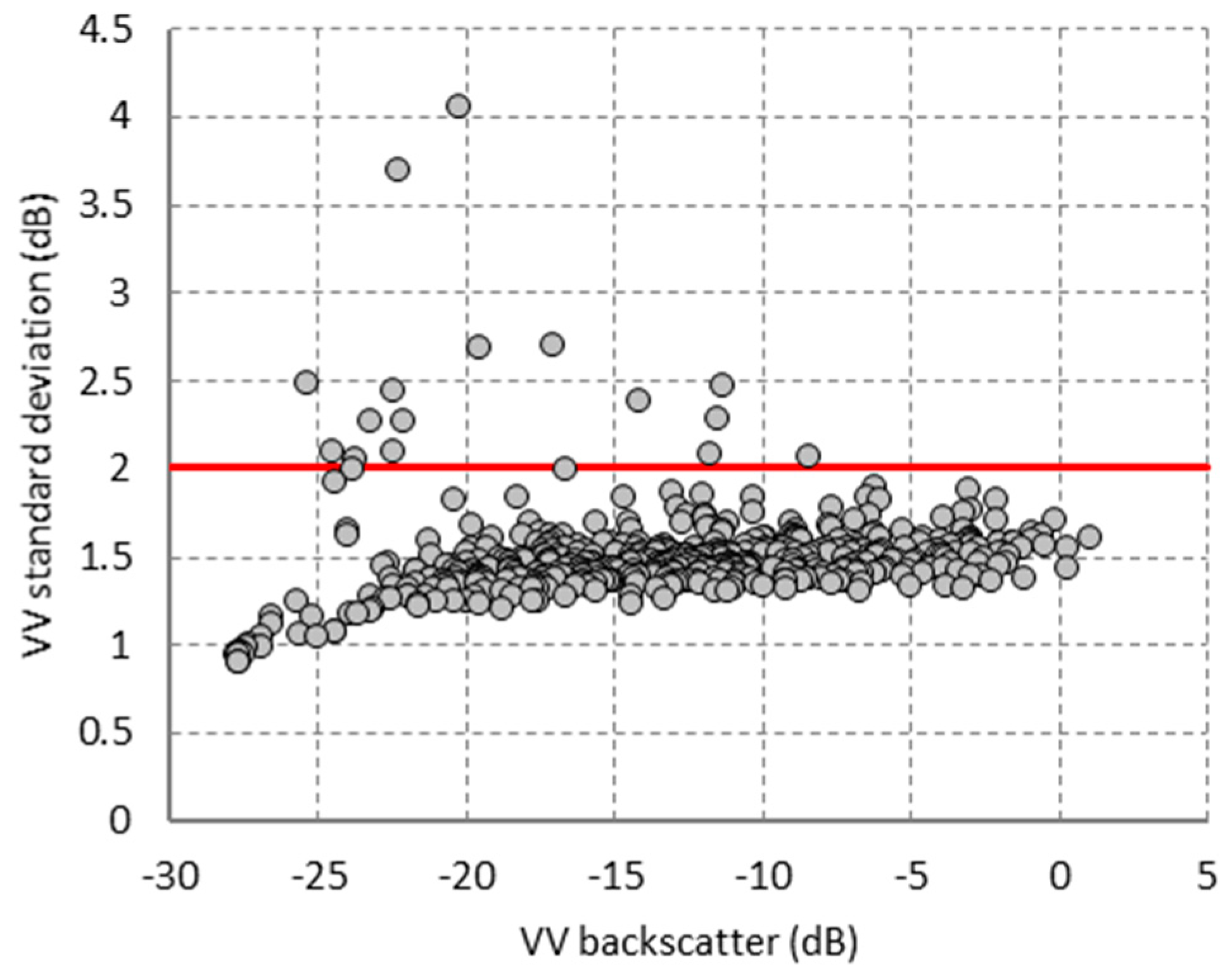
An analysis of σ⁰_VV standard deviation values shows that a number of samples exhibited relatively high variability compared to the bulk of the samples (Figure 2). An upper threshold for the acceptable spatial variability was set at two standard deviations above the mean:

$$\tau =\overline{x}+2s$$

(1)

where $\overline{x}$ is the mean of the σ⁰_VV standard deviation values and s is the standard deviation of the standard deviation values. A lower threshold is not needed, as low variability is desired. For example, for the LowNoise mode, the mean of the σ⁰_VV standard deviation values was 1.49 dB, and the standard deviation of the standard deviation values was 0.26 dB; thus $\tau =1.49+2\cdot 0.26=2.01$ dB. Samples ≥ τ were omitted: 16 samples for LowNoise (τ = 2.01 dB), 14 for LowRes (τ = 2.04 dB), and 14 for MR50 (τ = 2.17 dB).

2.2.2. Low-Quality Backscatter

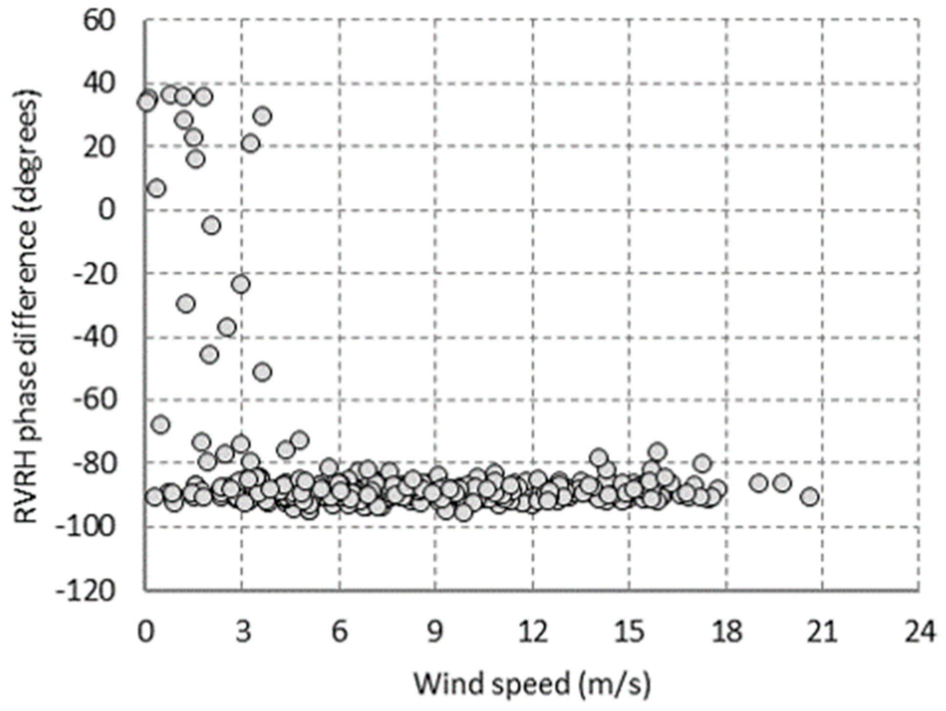
Low-quality backscatter exists in situations of low wind speed over water [20]. This results from the presence of wind slicks, either at the pixel level or as a portion of a spatially-averaged region of interest. Wind slicks occur when wind forces cannot overcome viscous forces, resulting in specular reflecting surfaces that do not exhibit the commonly-observed Bragg-scattering from water surfaces [24,25]. At C-band, this usually occurs at wind speeds <~3 m/s (Figure 3). Low-quality backscatter is caused by the contamination of the radar signal by antenna side lobes and by returns from nearby pixels [20].

Low-quality backscatter negatively affects the phase information of the radar return. This influences any algorithm development that includes such data, often causing non-linear relationships. Low-quality data should, therefore, be treated separately from high-quality data.

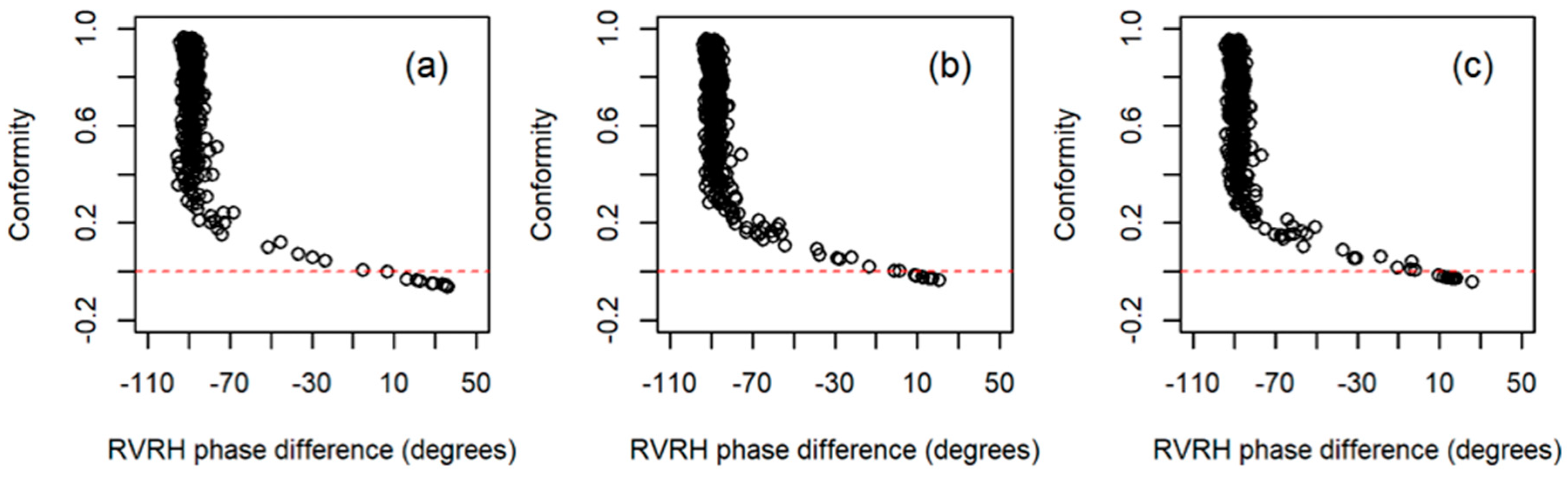
Low-quality backscatter can be identified using Conformity, ρ_RVRH, and/or δ_RVRH [19,20]. An analysis of the data shows that δ_RVRH and Conformity are closely related (Figure 4). A Conformity threshold ≤0 clearly identifies samples with highly divergent phase information, i.e., significant departures from the −90° value expected for open water. However, samples with conformity values as high as ~0.25 also appear to be associated with divergent phase values; these may also affect algorithm development.

Breakpoint analysis was used to identify the Conformity value at which data quality diverges. This was carried out using segmented regression, using all the samples remaining after the spatial variability constraint. The respective breakpoints were at Conformity values of 0.176 (LowNoise), 0.212 (LowRes) and 0.211 (MR50). The higher noise floor of the LowNoise mode resulted in fewer samples exhibiting low data quality, as expected. To ensure high quality data, a Conformity threshold of >0.2 (mean for three modes) was used. This is supported by the analysis of [20]. The Conformity threshold removed 19 samples from the LowNoise mose, 32 from the LowRes mode, and 31 from the MR50 mode.

2.3. Final Data Set

There was a very limited number of high-wind speed samples: only three samples (in each mode) were >17.8 m/s, and these did not have a sufficient incidence angle distribution. Therefore, these samples were removed, and analysis and model development were limited to wind speeds ≤18 m/s.

The final data set contained between 435 and 446 samples, depending on RCM mode (

Table 3. Summary of samples; numbers are approximate (mean of three modes) as they vary somewhat with mode: LowNoise (n = 446), LowRes (n = 435) and MR50 (n = 436).

Wind Speed/Inc. Angle	19°–29°	30°–39°	40°–49°
0–3.3 m/s	22	17	4
3.4–5.4 m/s	27	34	18
5.5–7.9 m/s	54	55	21
8.0–13.8 m/s	55	55	29
13.9–18 m/s	15	24	11

). Stratified random selection during sampling was used to ensure that the desired incidence angle ranges and wind speed ranges were sufficiently represented. The justification for the incidence angle ranges and wind speed ranges is outlined in [14].

2.4. CMOD Models

Two CMOD models were used in this study: CMOD-IFR2 [1] and CMOD5n [2]. Relative comparisons were made with σ⁰_VV, σ⁰_HH (using the polarization ratio (PR) of [5]), and the four CP parameters related to CMOD (σ⁰_RV, σ⁰_RH, σ⁰_RL, SV₀); the derivation for the CP parameters are described in [14]:

$${\sigma }_{RV}^0\approx 0.5CMOD$$

(2)

$${\sigma }_{RH}^0\approx 0.5CMOD/PR$$

(3)

$${\sigma }_{RL}^0\approx 0.25\left(CMOD+CMOD/PR\right)+0.5\sqrt{CMO{D}^2/PR}$$

(4)

$$S{V}_0\approx 0.5\left(CMOD+CMOD/PR\right)+CrossPol$$

(5)

where CrossPol is modelled based only on wind speed following [5].

Noise reduction was used in order to compare observed backscatter with CMOD5n-modelled values because CMOD5n was developed with noise subtracted. Both the RCM simulator mode nominal noise floor and the original Rdarasat-2 FQ noise floor were subtracted from the observed backscatter. A further 3 dB was subtracted to account for the noise floor pattern of FQ images, which was lower towards the centre of an image [14]. No RCM simulator or RADARSAT-2 FQ noise reduction was used for CMOD-IFR2, as it appeared that no noise subtraction was used during its development; only the 3 dB noise floor pattern value was subtracted.

2.5. Wind Speed Retrieval

Wind speed retrieval was performed by inverting the backscatter models. This was accomplished by beginning at two extreme wind speeds (low and high), then incrementing or decrementing the wind speed (by 0.01 m/s) until an observed parameter value was reached. Both the incrementing and decrementing methods must converge at a similar value (within 1 m/s) for a retrieval to occur. The difference between the two methods is usually ≤0.03 m/s. The resulting retrieval is the average of the incrementing and decrementing results.

If the difference between the two methods is >1 m/s, this indicates that the model does not exhibit a monotonic relationship with wind speed. This can result in the retrieval of two significantly different wind speeds, and thus in a lack of convergence. No retrieval occurs in such cases.

Wind speed retrievals < 0 m/s or > 18 m/s occasionally occurred, even though the data set was restricted to values ≤ 18 m/s. This was due the incomplete statistical representation of the model and the stochastic nature of the data. We omitted retrievals < 0 m/s and > 20 m/s.

2.6. Wind Speed Accuracy Assessment

Wind speed accuracy assessment was done by comparing the parameter-modelled wind speed with the buoy-measured wind speed. This was assessed using statistical measures: Spearman’s correlation, Root-Mean-Square Error (RMSE), slope (and intercept), and overall bias.

3. Results

3.1. CMOD Assessment

The association of observed backscatter with CMOD-IFR2- and CMOD5n-modelled σ⁰_RV, σ⁰_RH, σ⁰_RL and SV₀ provided similar statistics to σ⁰_VV and σ⁰_HH (Figure 5,

Table 4. Association of observed backscatter with CMOD-IFR2- and CMOD5n-modelled backscatter for RCM-simulated LowNoise data (n = 446).

	Parameter	Spearman’s ρ	RSE (dB)	Intercept	Slope	Bias
CMOD−IFR2	σ0VV	0.96	1.79	−0.60	0.98	−0.42
	σ0HH	0.97	1.82	−0.57	0.97	−0.16
	σ0RV	0.96	1.74	−0.91	0.95	−0.14
	σ0RH	0.97	1.76	−1.18	0.91	0.26
	σ0RL	0.96	1.81	−0.53	1.00	−0.49
	SV0	0.96	1.74	−0.78	0.94	−0.04
CMOD5n	σ0VV	0.94	2.17	−0.25	0.97	0.11
	σ0HH	0.96	2.31	0.63	1.04	0.03
	σ0RV	0.94	2.21	0.02	1.00	0.07
	σ0RH	0.96	2.69	1.74	1.11	−0.20
	σ0RL	0.95	2.26	0.23	1.03	−0.13
	SV0	0.95	2.07	−0.37	0.94	0.46

). The Spearman correlations for CMOD-IFR2 were ~0.96 and the RSE values were ~1.78; slopes were ~0.96 and biases were generally negative, except for σ⁰_RH. For CMOD5n, the Spearman correlations were ~0.95 and the RSE values were ~2.29; slopes were ~1.02 and biases were generally positive, except for σ⁰_RH and σ⁰_RL.

3.2. Wind Speed Retrieval

CMOD-related parameters have dependencies with incidence angle, wind speed, and wind direction. Therefore, the use of these models for wind speed retrieval necessitates a priori knowledge of wind direction. Buoy measurements are the source of wind direction for the wind speed retrieval tests.

The model comparison focused on the RMSE and slope statistics, because together, they described most of the models’ efficacy (

Table 5. Wind retrieval accuracies for the C-band models (CMOD). The green cells indicate the best three values for RMSE and slope in each RCM mode.

	RMSE (m/s)		Slope
Parameter	CMOD-IFR2	CMOD5n	CMOD-IFR2	CMOD5n
LowNoise
σ0VV	2.51	2.17	0.70	0.65
σ0HH	2.54	2.37	0.75	0.75
σ0RV	2.50	2.24	0.69	0.67
σ0RH	2.58	2.49	0.74	0.79
σ0RL	2.49	2.25	0.71	0.68
SV0	2.50	2.19	0.71	0.68
LowRes
σ0VV	2.40	2.26	0.76	0.72
σ0HH	2.42	2.44	0.81	0.81
σ0RV	2.40	2.35	0.75	0.75
σ0RH	2.52	2.62	0.80	0.84
σ0RL	2.42	2.35	0.77	0.75
SV0	2.38	2.22	0.76	0.74
MR50
σ0VV	2.25	2.22	0.76	0.73
σ0HH	2.31	2.36	0.81	0.81
σ0RV	2.26	2.20	0.75	0.74
σ0RH	2.37	2.51	0.79	0.84
σ0RL	2.28	2.27	0.78	0.75
SV0	2.25	2.13	0.77	0.75

). When averaging all the parameters, the lowest RMSE values occurred in the MR50 mode, and the best slopes were also in the MR50 mode. When averaging each parameter across the three modes, CMOD5n-SV₀ had the lowest RMSE, followed by CMOD5n-σ⁰_VV and CMOD5n-σ⁰_RV (Figure 6). CMOD5n-σ⁰_RH also seemed to perform relatively well at high wind speeds; however, its overall variability was greater.

3.3. RCM SAR Wind Case Studies

Three image-based case studies illustrate the applications of RCM CP and linear wind retrieval models.

Case 1 illustrates retrievals within an FQ image for a small incidence angle (Figure 7). The small extent of the FQ images (~25 × 25 km) limits wind speeds to a narrow range of values. Therefore, the colour scale is relative to the range of the wind speeds retrieved for the image. Wind direction input to the model comes from the buoy data located within the image (buoy 44141).

The original image was a RADARSAT-2 FQ3 image (incidence angle 20.9°–22.9°). The first eight pixels along the near-range side of the original image were affected by a filter artifact caused by the simulator and were thus removed prior to wind retrieval. The image was resampled to a 1 km pixel spacing. The wind speed retrieval model used was CMOD-IFR2-σ⁰_RV. The resulting image was trimmed to avoid stepped edges. The related buoy wind speed was 15 m/s from a relative wind direction of 206°.

Operational wind speed retrieval at the NSW programme primarily use wide-swath RCM data, in either linear or CP modes. Cases 2 and 3 in Figure 8 illustrate CMOD-IFR2-σ⁰_VV retrievals for full swath MR50 data with a 20 m pixel spacing. These data were simulated from RADARSAT-2 ScanSAR-Narrow data. Wind direction input to the model used Regional Deterministic Prediction System data with a ~10 km spacing [26]. Case 2 represents a gradual gradient in the wind field (Figure 8a), and Case 3 a complex wind field (Figure 8b).

4. Discussion

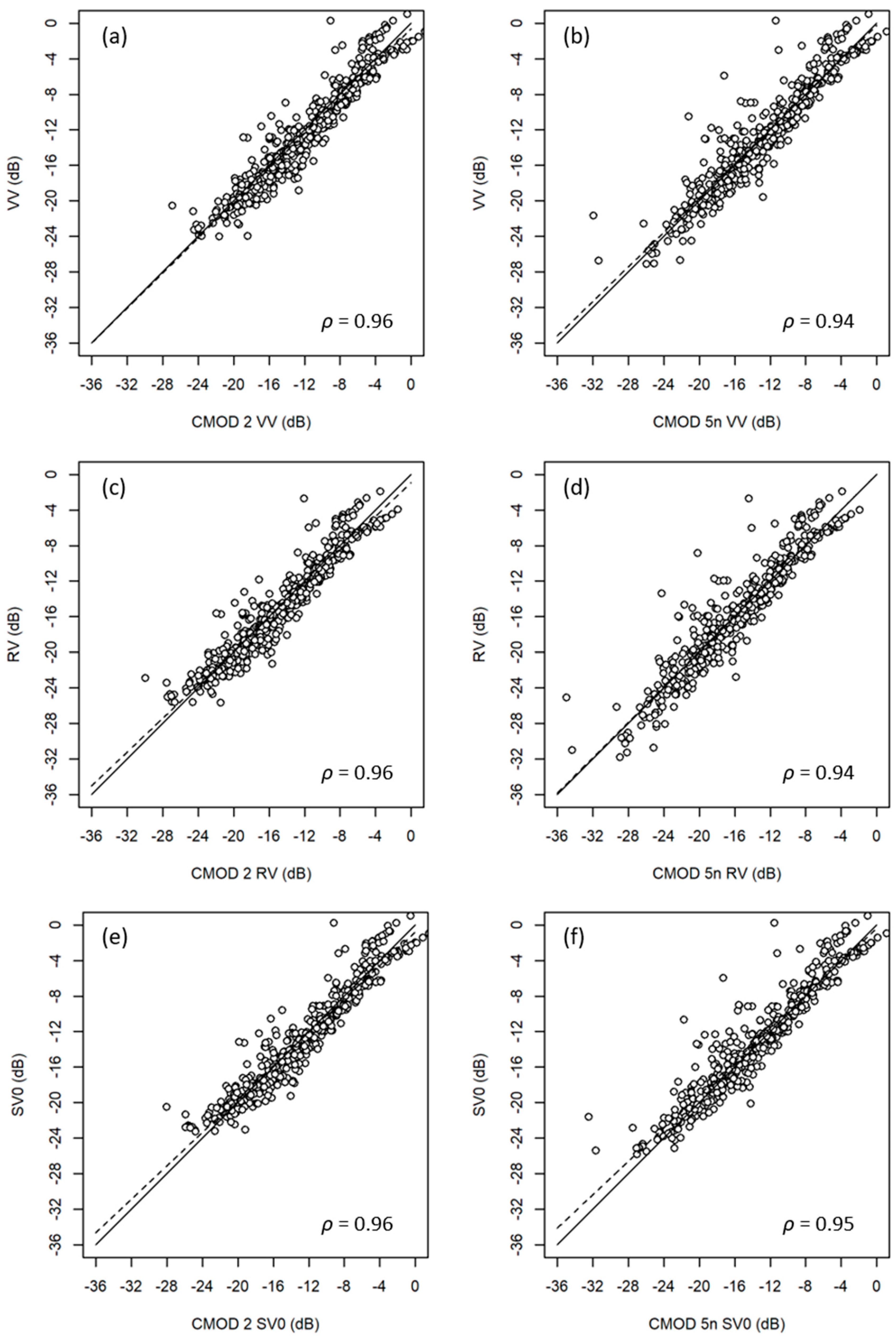
The strong correlations between simulated RCM backscatter and CMOD-modelled backscatter (based on SAR image incidence angle, and buoy wind speed and direction) provide evidence that both CMOD-IFR2- and CMOD5n-modelled parameters are appropriate for SAR wind speed retrieval within operations such as the NSW system (Table 4). CMOD-IFR2-modelled backscatter is generally more biased than CMOD5n-modelled backscatter, and the biases are more negative; these observations are consistent with previous comparisons [2]. Of the CP parameters, σ⁰_RV exhibited consistently good statistics, with relatively low RSE values, slopes near 1, and low absolute biases for both models. These are comparable with the results for σ⁰_VV. Given the general similarity in the correlation values between the linear and CP parameters, the analysis supports the use of CP parameters in lieu of linear parameters, should only CP parameters be available.

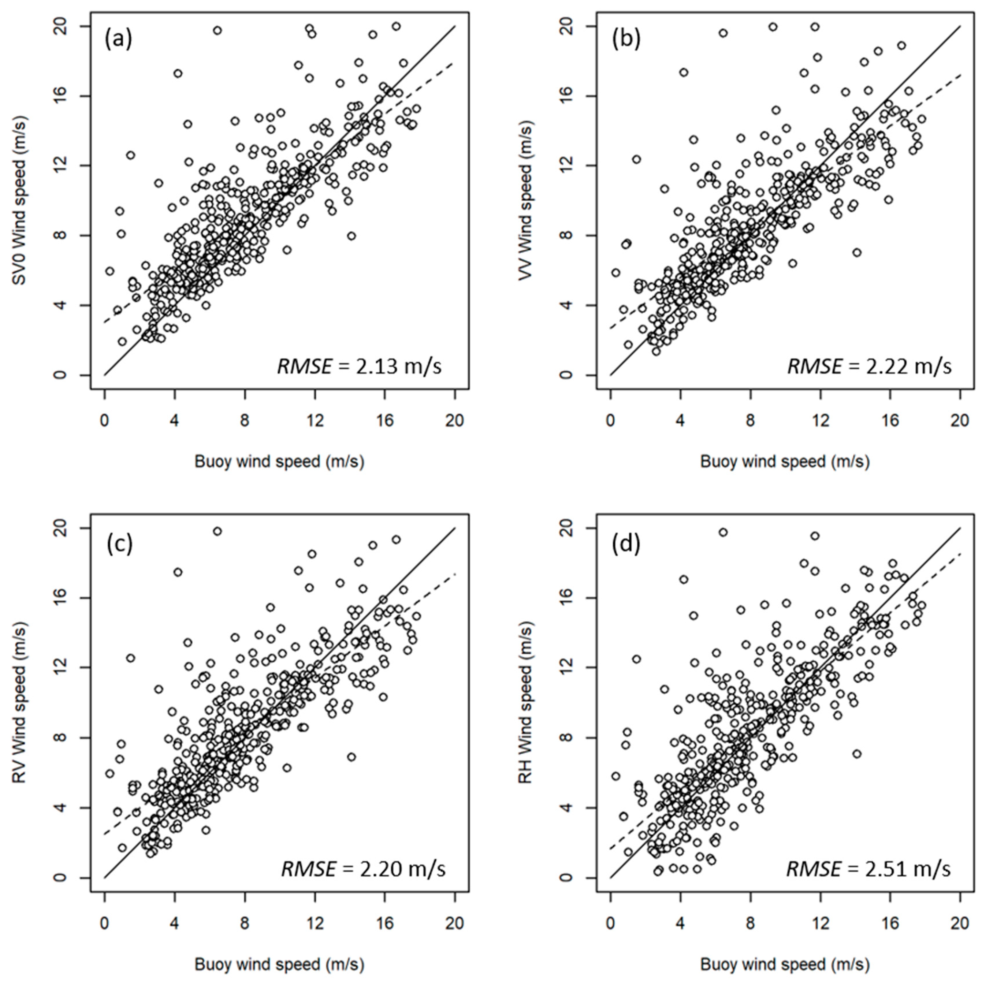
The wind speed retrievals exhibited a general overestimation at low wind speeds and underestimation at high wind speeds (Figure 6), leading to slope values <1 (Table 5). For the CP parameters, this was most prevalent for σ⁰_RV and least prevalent for σ⁰_RH, with σ⁰_RL, exhibiting a compromise between the two. Overall, CMOD5n-SV₀ had the lowest RMSE values in the MR50 and LowRes modes and was only bested by CMOD5n-σ⁰_VV in the LowNoise mode. The skill of CMOD5n-SV₀ was likely the result of its cross-polarized component, which compensated somewhat for the wind speed underestimation of the co-polarized components at high wind speeds. The cross-polarized contribution can likely be improved by using a more nuanced model than the Vachon and Wolfe [5] model used in this study. This may make the CMOD5n-SV₀ retrieval even better. The similarity in slope values between CMOD-IFR2 and CMOD5n was the result of appropriate handling of the noise values: minimal noise reduction in the case of CMOD-IFR2 and significant noise reduction in the case of CMOD5n. Once RCM mode noise values are known, following launch and commissioning, mode-specific noise reduction analysis will be needed to obtain robust retrievals.

All model results were within the accuracy range reported for SAR wind retrieval: between 1.5 and 2.7 m/s [5,6,27,28,29]. Although CMOD5n models usually had better RMSE values than CMOD-IFR2 models, the mean difference across all parameters and modes was only 0.1 m/s. These results provide additional evidence that CMOD-IFR2- and CMOD5n-modelled CP parameters can be used with confidence, instead of CMOD-σ⁰_VV models, when only CP data are available.

Although the accuracies reported in this study were adequate, they did not achieve RMSE <2 m/s. A number of factors that may have caused the somewhat reduced accuracy, including (1) the temporal mismatch between SAR acquisition and buoy wind speed measurement, (2) the buoy wind direction measurements may not have always been representative of the 3 × 3 km sample area, (3) the addition of noise by the simulator, and subsequent noise reduction, may have added error, and (4) the use of a relatively simple retrieval technique. Higher accuracy can likely be achieved with more sophisticated retrieval schemes; however, the relative accuracy between the linear and CP parameters was of interest in this study. Once actual RCM data are available, greater effort will be devoted to increasing the retrieval accuracy.

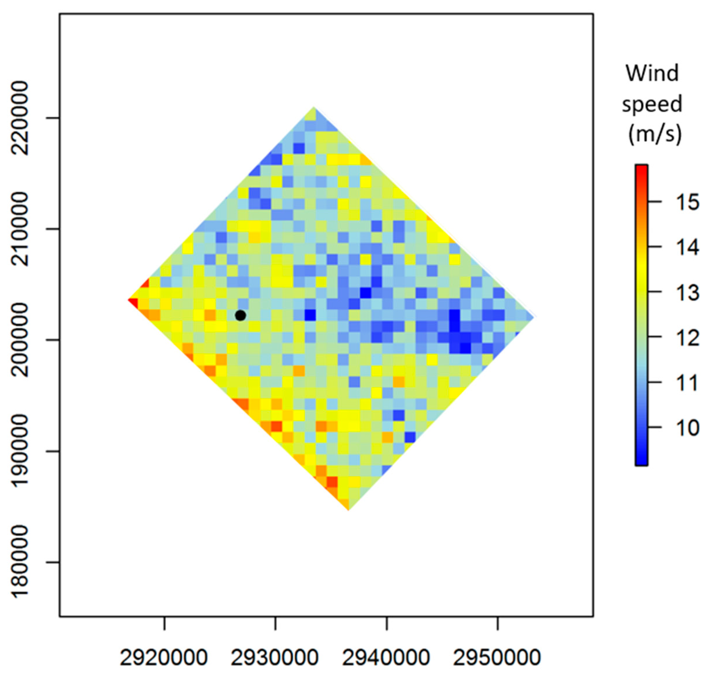
The wind speed retrieval at the buoy location (buoy 44141) in Case 1 (Figure 7) was underestimated (11.6 m/s versus a buoy measurement of 15.0 m/s). However, the wind speed gradient in the image was quite strong and the 12-minute temporal mismatch between the buoy measurements and the SAR acquisition can account for this discrepancy. The greater prevalence of higher wind speed retrievals along the near-range edge (left side), and to a lesser degree, the far-range edge, may be representative of the actual wind pattern. However, this may also be due to the noise floor pattern of RADARSAT-2 FQ scenes, which was higher at the near- and far-range edges. Furthermore, on the near-range side, there may also have been remnant filter artifact effects. Further research is needed to isolate the actual cause(s). 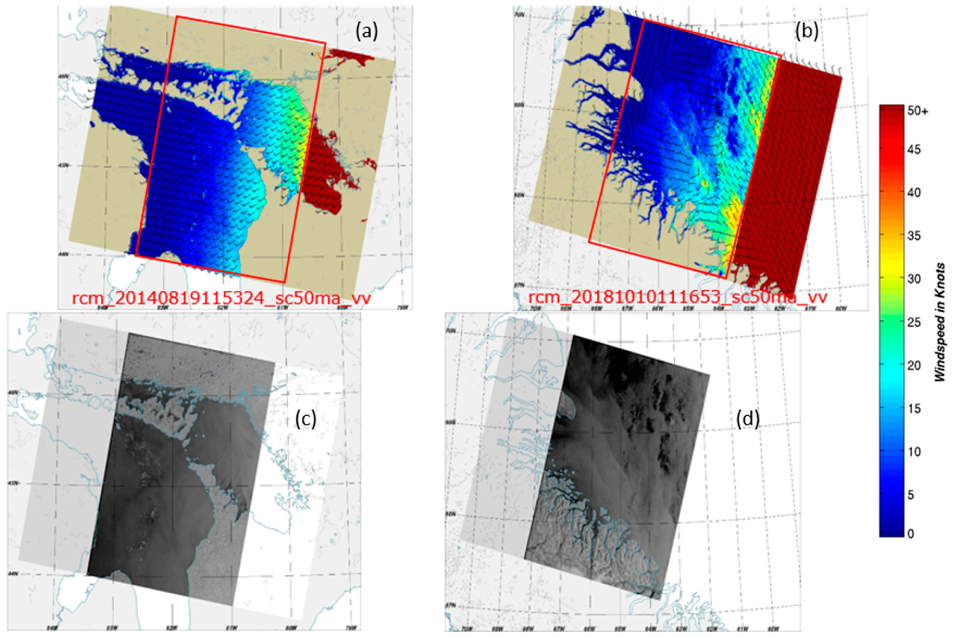However, the retrieval in Figure 7 is solely illustrative of a retrieval within the small areal extent (25 × 25 km) of a RADARSAT-2 FQ image, and does not reflect the scale of the operational systems, which are not constrained by such small swath widths. The operational swath width images shown in Figure 8 illustrate retrievals with the RCM MR50 mode (350 km wide); these are able to resolve complex wind fields and provide retrievals in convoluted coastlines over large geographic extents. Nevertheless, noise effects are likely to be a limiting factor and must be carefully considered once actual RCM data become available.

5. Conclusions

In this study, a set of 504 RADARSAT-2 FQ images was used to simulate RCM image modes, in order to sample CP parameters over meteorological buoy locations on the West and East coasts of Canada. Three RCM modes were simulated: Low Noise, Low Resolution 100 m, and Medium Resolution 50 m. These samples were used to evaluate the efficacy of CMOD-related CP (CMOD-CP) parameters (σ⁰_RV, σ⁰_RH, σ⁰_RL and SV₀) for wind speed retrieval, using CMOD-IFR2 and CMOD5n. CMOD-CP accuracy was compared to CMOD results for σ⁰_VV and σ⁰_HH.

To ensure a high-quality data set, a data quality threshold was established using the CP parameters Conformity and RVRH phase difference. A Conformity threshold value of 0.2 was obtained via break-point analysis, and found to be reasonably consistent for the three RCM modes considered.

Modelled CMOD-CP backscatter was found to be highly correlated with simulated RCM CP backscatter. Both CMOD-IFR2 and CMOD5n were suitable for generating CMOD-CP parameters, should linear parameters be unavailable, as will be the case with RCM CP data.

The wind retrieval accuracies of CMOD-SV₀ and CMOD-σ⁰_RV were as good as, or better than, the accuracy of CMOD-σ⁰_VV. This applied to both CMOD-IFR2 and CMOD5n. CMOD5n-SV₀ was the best CMOD-CP parameter, with accuracy values of 2.13 m/s to 2.22 m/s, depending on the RCM mode; the Medium Resolution 50 m mode had the best accuracy. Therefore, CMOD-CP parameters, and CMOD5n-SV₀ and CMOD5n-σ⁰_RV, in particular, can be substituted for CMOD-σ⁰_VV when linear data are unavailable.

This study provides significant results for marine surface wind speed retrieval using RCM data, and for the transition of the operational NSW system from RADARSAT-2 to RCM SAR data. The effect of noise is a controlling factor for marine surface wind retrievals. A careful reanalysis must be done when RCM is launched to assess the actual noise floors. However, the relative errors should remain similar. RCM’s three satellites, in addition to the existing RADARSAT-2, Sentinel-1A and Sentinel-1B, will provide spatial and temporal coverage that will foster new research and development in marine surface wind field estimation. After the launch of RCM, a study will be carried out with actual RCM SAR data to further evaluate the potential of the CP parameters.