Analytical Approximation Model for Quadratic Phase Error Introduced by Orbit Determination Errors in Real-Time Spaceborne SAR Imaging

Abstract

Research on real-time spaceborne synthetic aperture radar (SAR) imaging has emerged as satellite computation capability has increased and applications of SAR imaging products have expanded. The orbit determination data of a spaceborne SAR platform are essential for the SAR imaging procedure. In real-time SAR imaging, onboard orbit determination data cannot achieve a level of accuracy that is equivalent to the orbit ephemeris in ground-based SAR processing, which requires a long processing time using common ground-based SAR imaging procedures. It is important to study the influence of errors in onboard real-time orbit determination data on SAR image quality. Instead of the widely used numerical simulation method, an analytical approximation model of the quadratic phase error (QPE) introduced by orbit determination errors is proposed. The proposed model can provide approximation results at two granularities: approximations with a satellite’s true anomaly as the independent variable and approximations for all positions in the satellite’s entire orbit. The proposed analytical approximation model reduces simulation complexity, extent of calculations, and the processing time. In addition, the model reveals the core of the process by which errors are transferred to QPE calculations. A detailed comparison between the proposed method and a numerical simulation method proves the correctness and reliability of the analytical approximation model. With the help of this analytical approximation model, the technical parameter iteration procedure during the early-stage development of an onboard real-time SAR imaging mission will likely be accelerated.

1. Introduction

Real-time synthetic aperture radar (SAR) imaging has always been a research focus in certain applications. Real-time imaging enhances the effectiveness and widens the application range of the SAR technique. In airborne SAR, real-time sensing plays an important role, and there are many well-established systems [1,2,3,4,5] and techniques [6,7,8,9,10,11]. Real-time processing techniques are also available for unmanned aerial vehicle (UAV) SAR applications [12,13,14]. For spaceborne SAR, because of its unique configuration and onboard computation capabilities, real-time SAR imaging systems and techniques are still being developed for both digital [15,16,17] and optical [18] methods.

For the purpose of implementing onboard real-time spaceborne SAR imaging, a set of Doppler parameters with high precision and accuracy must be calculated, and accurate position and velocity vectors are needed for the Doppler parameter calculation. In typical methods used to process SAR echo data, a high-accuracy orbit ephemeris is applied in the ground-based processing system, and state vectors, i.e., position and velocity vectors of the SAR satellite, are determined with high accuracy. However, this kind of high-accuracy orbit ephemeris is only generated hours, days, or even weeks after a single SAR observation [19]. Thus, this kind of high-accuracy orbit ephemeris cannot be obtained during real-time SAR imaging. Nevertheless, we are still able to achieve onboard orbit determination using GNSS-based receivers and appropriate algorithms [20,21]. It is acknowledged that this approach to orbit determination has relatively low accuracy in the state vectors of SAR satellites compared with the high-accuracy orbit ephemeris. However, it remains the best, and possibly the only, onboard orbit determination method that is available for real-time SAR imaging.

SAR mission designers must account for the fact that errors in such onboard orbit determination data will adversely affect the quality of the SAR imaging product through inaccurate Doppler parameter calculation. Although estimation algorithms have been developed to generate the Doppler centroid and Doppler rate with high accuracy for SAR imaging, they are time-consuming in practice. Real-time spaceborne SAR imaging certainly does not belong on a mission that is not time-sensitive. The product of real-time SAR imaging may be the source data for other mission types, such as onboard deformation monitoring or target recognition. Given these requirements, the estimation algorithm should not be built into the processing workflow because of its long processing time. Thus, the concept of quadrature phase error (QPE) is introduced to evaluate the influence of onboard orbit determination errors on spaceborne SAR imaging products. The azimuth impulse response width of a SAR image has a certain relationship with QPE, and it provides a more intuitive evaluation standard of the errors.

Errors of an onboard orbit determination system are often given in the form of probabilities, along with the type of probability distributions and the corresponding parameters. The most common case for these errors is a normal distribution with an expected value of zero and a standard deviation $\sigma$. Therefore, the probability distribution of QPE needs to be examined. In practice, there exist two major methods that have been applied to QPE analysis, i.e., the extreme value method and the numerical simulation method. The extreme value method is the simplest way to investigate QPE; it includes the maximum possible error in the calculation and ignores the probability distribution of the errors. This method faces challenges in revealing the QPE probability distribution, which means it only reflects the extreme situation in practice. For the numerical simulation methods, Monte Carlo simulations are often applied [22]. However, this approach requires a huge number of generated error samples and repeated experiments.

In this paper, an analytical approximation model of the QPE introduced by orbit determination errors is proposed. With the a priori probability of the onboard orbit determination system and SAR satellite orbit elements, together with the observing geometry of the spaceborne SAR and appropriate approximations, a series of equations describing the parameters of the QPE probability distribution are presented. This analytical approximation model can provide approximation results at two granularities, i.e., the approximations with the satellite’s true anomaly as the independent variable and the approximations for all positions of the satellite during its entire orbit.

Following this section, Section 2 describes the QPE analytical approximation model in general. Section 3 derives the key variables in the analytical approximation model and reveals the appropriate approximations in the model. This is followed by the evaluation of the analytical approximation model by comparing it with numerical simulation results in Section 4, and a related discussion is presented in Section 5. Finally, Section 6 provides a brief conclusion regarding the analytical approximation model.

2. Proposed Model: QPE Analytical Approximation Model

The QPE analytical approximation model requires four groups of parameters as input, i.e., the Earth’s physical parameters, the satellite platform orbit parameters, the SAR payload key parameters, and the a priori probability of the onboard orbit determination system. In this section, the coordinate systems, vector in the line-of-sight method, and QPE approximation method in the proposed model are described.

2.1. Coordinate Systems for Modeling

Two main coordinate systems are used in the derivation of the analytical approximation model. These two coordinate systems can be helpful in generating a clear description of the relative movement of the spaceborne SAR and the point of interest on the surface of the Earth.

2.1.1. Earth-Centered Inertial Coordinate System

Generally, the QPE calculation requires the position, velocity, and acceleration coordinates of the spaceborne SAR platform and the SAR antenna aiming point on the Earth’s surface, together with other variables. A widely used coordinate system in modeling the relative motion between the spaceborne SAR and the point of interest is the Earth-Centered Inertial (ECI) coordinate system. This system has an x-axis and z-axis aligned with the mean equinox and the celestial North Pole, respectively. The y-axis forms a right-handed coordinate system that joins the x-axis and z-axis.

In common practice, the onboard GNSS-based orbit determination system of a spaceborne satellite calculates its positions in a given coordinate system using the GNSS broadcast message [21]. Each GNSS in service now has its own unique coordinate system, e.g., WGS 84 in GPS, CGCS2000 in BDS, and GTRF in Galileo. For modeling the orbit determination errors in the proposed analytical approximation model, all real-time-measured position and velocity coordinates of the spaceborne SAR platform are transformed into the ECI system in this paper.

2.1.2. Orbital Plane Coordinate System

The movement parameters of a spaceborne SAR satellite can be described in the orbital plane coordinate system. In this system, the Earth is located at one of the foci of the elliptical orbit, and the satellite can be regarded as a point. Polar coordinates are used to describe the movement parameters.

There exist six orbital elements that uniquely identify a specific orbit of the satellite: the semi-major axis a, eccentricity e, and true anomaly $\nu$ are used in the orbital plane coordinate system to determine the satellite’s movement at a certain time. The inclination i, the longitude of the ascending node $\Omega$, and the argument of periapsis $\omega$ are necessary to construct the transformation matrix between the orbital plane coordinate system and the ECI system.

The orbital plane coordinate system and the ECI system are summarized in Figure 1.

2.2. Vector in the Line-of-Sight Method

In the analytical approximation model presented in this paper, the attitude errors of the spaceborne SAR satellite are not taken into consideration. The true value of the attitude of the platform is used in both the analytical approach and the following numerical verification.

With this assumption, the vector in the line-of-sight (VLS) method can be used to calculate the state vectors of the point of interest. The relative range from the SAR antenna phase center to the point of interest can be derived from the time delay of the echo signal. For spaceborne SAR geometry, the echo signal enters the receiver after several pulse repetition intervals (PRIs) until the moment of transmission, and then it is demodulated and sampled by the receiver. In each range profile of the sampled data, each sampled time delay can be determined by the index number of its range gate. The signal transmission delay from the antenna phase center to the sampling ADCs in the receiver can be accurately measured in the state-of-the-art spaceborne SAR system. $t_{delay}$ represents the delayed time of the echo of the point-of-interest signal from its transmission time, and c represents the velocity of light, whose relative range is described by

$$\begin{array}{c}\hfill \rho ={\displaystyle \frac{c{t}_{delay}}{2}}\end{array}$$

(1)

A unit line-of-sight vector ${\widehat{\mathbf{u}}}_{a,ECI}$ in the ECI system can be created; it is perpendicular to the aperture of the SAR antenna and points to the surface of the Earth. The position vector ${\mathbf{P}}_{tar,ECI}$ and velocity vector ${\mathbf{V}}_{tar,ECI}$ of the point on the surface of the Earth at which the antenna points can be shown in stripmap SAR geometry as

$$\begin{array}{cc}\hfill {\mathbf{P}}_{tar,ECI}& ={\mathbf{P}}_{sat,ECI}+\rho ·{\widehat{\mathbf{u}}}_{a,ECI}=\left[\begin{array}{c}{P}_{tar,ECI,x}\\ P_{tar,ECI,y}\\ P_{tar,ECI,z}\end{array}\right]\hfill \end{array}$$

(2)

$$\begin{array}{cc}\hfill {\mathbf{V}}_{tar,ECI}& =\left[\begin{array}{c}-{\omega }_e·P_{tar,ECI,y}\\ {\omega }_e·P_{tar,ECI,x}\\ 0\end{array}\right]\hfill \end{array}$$

(3)

in which ${\omega }_e$ is the angular speed of the Earth’s rotation.

Because there are errors in the satellite’s position and velocity measurements from the onboard GNSS-based orbit determination system, the calculated ${\mathbf{P}}_{tar,ECI}$ and ${\mathbf{V}}_{tar,ECI}$ will also contain errors at the same time. The relative range $\rho$ remains unaffected because errors exist in measurements while the real geometry remains unchanged, which means that the time delay remains equal to the accuracy value.

2.3. QPE Approximation

QPE can be expressed in radians as [23]

$$\begin{array}{cc}\hfill \mathrm{QPE}& =\pi \Delta f_r{\left({\displaystyle \frac{T_{int}}{2}}\right)}^2\hfill \end{array}$$

(4)

in which $f_r$ is the Doppler rate of the echo signal, and $T_{int}$ represents the integration time, also known as the synthetic-aperture time. In stripmap SAR geometry, the integration time is the time it takes the point of interest to enter and exit the entire 3 dB edge of the SAR antenna’s beam illumination.

The variables ${\mathbf{R}}_{st}$, ${\mathbf{V}}_{st}$, and ${\mathbf{A}}_{st}$ represent the relative position, velocity, and acceleration of the spaceborne SAR satellite, respectively. In the ECI system, for the antenna aiming point on the ground, the commonly used $f_r$ expression in stripmap mode when the squint angle equals zero is

$$\begin{array}{cc}\hfill f_r& ={\displaystyle \frac{2}{\lambda }}\left[{\displaystyle \frac{{\mathbf{V}}_{st}·{\mathbf{V}}_{st}}{\left|{\mathbf{R}}_{st}\right|}}+{\displaystyle \frac{{\mathbf{A}}_{st}·{\mathbf{R}}_{st}}{\left|{\mathbf{R}}_{st}\right|}}-{\displaystyle \frac{{\left({\mathbf{V}}_{st}·{\mathbf{R}}_{st}\right)}^2}{{\left|{\mathbf{R}}_{st}\right|}^3}}\right]\hfill \end{array}$$

(5)

The $f_r$ expression in Equation (5) is an approximation expression, and it can achieve high precision if more terms remain. In the analytical approximation model, only the first two terms in Equation (5) are analyzed. This simplifies the model while retaining a relatively high precision.

The orbit determination system measurements contain errors, which will lead to errors in ${\mathbf{R}}_{st}$, ${\mathbf{V}}_{st}$, and ${\mathbf{A}}_{st}$. The terms that define the differences between the state vectors derived from measurements and the true state vectors are

$$\begin{array}{cc}\hfill \Delta {\mathbf{R}}_{st}& ={\mathbf{R}}_{st,e}-{\mathbf{R}}_{st}\hfill \end{array}$$

(6)

$$\begin{array}{cc}\hfill \Delta {\mathbf{V}}_{st}& ={\mathbf{V}}_{st,e}-{\mathbf{V}}_{st}\hfill \end{array}$$

(7)

$$\begin{array}{cc}\hfill \Delta {\mathbf{A}}_{st}& ={\mathbf{A}}_{st,e}-{\mathbf{A}}_{st}\hfill \end{array}$$

(8)

where the subscript e indicates that the vectors contain measurement errors. Thus, the difference between the measured $f_r$ and true $f_r$ value is

$$\begin{array}{c}\hfill \Delta f_r=f_{r,e}-f_r\end{array}$$

(9)

The parameter $f_r$ in Equation (5) is often used to determine the precise value for SAR raw data simulation or imaging algorithms. For the approximate expression of QPE, considering the magnitude of each term in $f_r$, some terms can be omitted while still achieving an acceptable approximation of QPE. The VLS method in Section 2.2 maintains the real value of the relative range $\rho =\left|{\mathbf{R}}_{st}\right|$. Thus, Equation (4) combined with Equation (9) gives the QPE approximation expression

$$\begin{array}{cc}\hfill \mathrm{QPE}& =\pi \left(f_{r,e}-f_r\right){\left({\displaystyle \frac{T_{int}}{2}}\right)}^2\hfill \\ & \approx {\displaystyle \frac{2\pi }{\lambda \rho }}\left(2\Delta {\mathbf{V}}_{st}·{\mathbf{V}}_{st}+\Delta {\mathbf{A}}_{st}·{\mathbf{R}}_{st}\right){\left({\displaystyle \frac{T_{int}}{2}}\right)}^2\hfill \end{array}$$

(10)

For convenience, the terms $\Delta {\mathbf{V}}_{st}·{\mathbf{V}}_{st}$ and $\Delta {\mathbf{A}}_{st}·{\mathbf{R}}_{st}$ are named velocity and acceleration vector term in the following sections.

The approximation of QPE in Equation (10) is the basis of the QPE analytical approximation function and maximum QPE derivation.

3. Key Variables in the Analytical Approximation Model

For a given true anomaly $\nu$, the distance between the satellite and the Earth’s center is

$$\begin{array}{cc}\hfill r& ={\displaystyle \frac{a\left(1-e^2\right)}{1+ecos\nu }}={\displaystyle \frac{p}{1+ecos\nu }}\hfill \end{array}$$

(11)

where $p=a\left(1-e^2\right)$ in Equation (11) is the semi-latus rectum of the elliptic orbit. The position, velocity, and acceleration vectors of the satellite in the orbital plane (OP) are

$$\begin{array}{cc}\hfill {\mathbf{P}}_{sat,OP}& =r\left[\begin{array}{c}cos\nu \\ sin\nu \\ 0\end{array}\right]\hfill \end{array}$$

(12)

$$\begin{array}{cc}\hfill {\mathbf{V}}_{sat,OP}& =\sqrt{{\displaystyle \frac{\mu }{p}}}\left[\begin{array}{c}-sin\nu \\ e+cos\nu \\ 0\end{array}\right]\hfill \end{array}$$

(13)

$$\begin{array}{cc}\hfill {\mathbf{A}}_{sat,OP}& =-{\displaystyle \frac{\mu {\left(1+ecos\nu \right)}^2}{p^2}}\left[\begin{array}{c}cos\nu \\ sin\nu \\ 0\end{array}\right]\hfill \end{array}$$

(14)

where $\mu$ is the standard gravitational parameter of the Earth.

The transformation matrix $A_{O2E}$ is used to convert the vector in the orbital plane to the ECI system:

$${\mathbf{A}}_{O2E}=\left[\begin{array}{ccc}cos\omega & -sin\omega & 0\\ sin\omega & cos\omega & 0\\ 0& 0& 1\end{array}\right]\left[\begin{array}{ccc}1& 0& 0\\ 0& cosi& -sini\\ 0& sini& cosi\end{array}\right]\left[\begin{array}{ccc}cos\Omega & -sin\Omega & 0\\ sin\Omega & cos\Omega & 0\\ 0& 0& 1\end{array}\right]$$

(15)

The parameter $\Omega$ in ${\mathbf{A}}_{O2E}$ results in rotation with the z-axis in the ECI system. Considering the geometry and the Earth’s ellipsoid reference, in the following discussion, we set $\Omega =0$ for convenience, and this will not result in an error value in the QPE approximation.

The onboard orbit determination system measurements are given in ECI terms, which can be regarded as the true state vector plus an error vector. With the assumption that the measurement errors of the satellite’s position and velocity follow a normal distribution with an expected value of 0, the error vectors can be described as

$$\begin{array}{cc}\hfill \Delta \mathbf{P}& =\left[\begin{array}{c}\Delta p_x\\ \Delta p_y\\ \Delta p_z\end{array}\right]\sim \left[\begin{array}{c}N\left(0,{\sigma }_{p,x}^2\right)\\ N\left(0,{\sigma }_{p,y}^2\right)\\ N\left(0,{\sigma }_{p,z}^2\right)\end{array}\right]\hfill \end{array}$$

(16)

$$\begin{array}{cc}\hfill \Delta \mathbf{V}& =\left[\begin{array}{c}\Delta v_x\\ \Delta v_y\\ \Delta v_z\end{array}\right]\sim \left[\begin{array}{c}N\left(0,{\sigma }_{v,x}^2\right)\\ N\left(0,{\sigma }_{v,y}^2\right)\\ N\left(0,{\sigma }_{v,z}^2\right)\end{array}\right]\hfill \end{array}$$

(17)

Then, the state vector measurements of the satellite are

$$\begin{array}{cc}\hfill {\mathbf{P}}_{sat,ECI,e}& ={\mathbf{A}}_{O2E}{\mathbf{P}}_{sat,OP}+\Delta \mathbf{P}\hfill \end{array}$$

(18)

$$\begin{array}{cc}\hfill {\mathbf{V}}_{sat,ECI,e}& ={\mathbf{A}}_{O2E}{\mathbf{V}}_{sat,OP}+\Delta \mathbf{V}\hfill \end{array}$$

(19)

From Equations (2), (3), (18) and (19), the position vectors of the antenna aiming point are

$$\begin{array}{cc}\hfill {\mathbf{P}}_{tar,ECI,e}& ={\mathbf{P}}_{sat,ECI,e}+\rho ·{\widehat{u}}_{a,ECI}\hfill \end{array}$$

(20)

With the help of Equations (3), (19) and (20), the difference in the relative velocity from the satellite to the antenna aiming point can be given as

$$\begin{array}{cc}\hfill \Delta {\mathbf{V}}_{st}& =\left({\mathbf{V}}_{sat,ECI,e}-{\mathbf{V}}_{tar,ECI,e}\right)-\left({\mathbf{V}}_{sat,ECI}-{\mathbf{V}}_{tar,ECI}\right)=\left[\begin{array}{c}\Delta v_x+{\omega }_e\Delta p_y\\ \Delta v_y-{\omega }_e\Delta p_x\\ \Delta v_z\end{array}\right]\hfill \end{array}$$

(21)

3.1. The Velocity Vector Term in the Approximate Doppler Rate

With Equation (21), we have $\Delta {\mathbf{V}}_{st}$. However, we still need the expression of ${\mathbf{V}}_{st}$ to calculate the velocity vector term $\Delta {\mathbf{V}}_{st}·{\mathbf{V}}_{st}$. It is worth recalling that we need the approximate Doppler rate expression. To calculate the velocity vector term in Equation (10), we propose using the velocity vector of a satellite traveling in a circular orbit ${\mathbf{V}}_s$ in our analytical approximation model rather than using ${\mathbf{V}}_{st}$. Thus, we have

$$\begin{array}{cc}\hfill {\mathbf{V}}_{st}& ={\mathbf{A}}_{O2E}{\mathbf{V}}_{sat,OP}{|}_{e=0}\hfill \\ & =\sqrt{{\displaystyle \frac{\mu }{p}}}\left[\begin{array}{c}-sin\left(\nu +\omega \right)\\ cos\left(\nu +\omega \right)cosi\\ cos\left(\nu +\omega \right)sini\end{array}\right]\hfill \end{array}$$

(22)

The velocity vector term results in a Doppler rate difference by

$$\begin{array}{cc}\hfill \Delta f_{r,v}& ={\displaystyle \frac{2}{\lambda \rho }}·2\Delta {\mathbf{V}}_{st}·{\mathbf{V}}_{st}\hfill \\ & ={\displaystyle \frac{4}{\lambda \rho }}\sqrt{{\displaystyle \frac{\mu }{p}}}\left[-\left(\Delta v_x+{\omega }_e\Delta p_y\right)sin\left(\nu +\omega \right)\right.\hfill \\ & \left.+\left(\Delta v_y-{\omega }_e\Delta p_x\right)cos\left(\nu +\omega \right)cosi+\Delta v_{z}cos\left(\nu +\omega \right)sini\right]\hfill \end{array}$$

(23)

Assuming that the variances of the position and velocity errors are the same standard deviation in the x-, y-, and z-direction in the ECI system, i.e., ${\sigma }_{p,x}={\sigma }_{p,y}={\sigma }_{p,z}={\sigma }_p$ and ${\sigma }_{v,x}={\sigma }_{v,y}={\sigma }_{v,z}={\sigma }_v$, we can find the expected value and standard deviation of $\Delta f_{r,v}$ by

$$\begin{array}{cc}\hfill \mathbb{E}\left[\Delta f_{r,v}\right]& =0\hfill \end{array}$$

(24)

$$\begin{array}{cc}\hfill \sigma \left[\Delta f_{r,v}\right]& ={\displaystyle \frac{4}{\lambda \rho }}\sqrt{{\displaystyle \frac{\mu }{p}}}\sqrt{{\sigma }_v^2+{\omega }_e^2\left[{sin}^2\left(\nu +\omega \right)+{cos}^2\left(\nu +\omega \right){cos}^{2}i\right]{\sigma }_p^2}\hfill \end{array}$$

(25)

We also need an approximate maximum value of the standard deviation of $\Delta f_{r,v}$ to calculate the approximate maximum value of QPE. We suppose that $cosi$ has a maximum value of $cosi=1$, and

$$\begin{array}{c}\hfill \sigma {\left[\Delta f_{r,v}\right]}_{max}={\displaystyle \frac{4}{\lambda \rho }}\sqrt{{\displaystyle \frac{\mu }{p}}}·\sqrt{{\omega }_e^2{\sigma }_p^2+{\sigma }_v^2}\end{array}$$

(26)

3.2. True Anomaly

Equation (21) gives the expression of difference vectors in the velocity vector term in Equation (10). However, the difference vector in the acceleration vector term, i.e., $\Delta {\mathbf{A}}_{st}$, is given its expression with the help of true anomaly calculation.

The accurate acceleration vector term in the orbital plane is given in Equation (14). True anomaly $\nu$ should be calculated using the onboard-measured satellite’s position and velocity vectors. A common way to solve $\nu$ is given in [24]

$$\begin{array}{c}\hfill \nu =2\left(\sqrt{{\displaystyle \frac{p}{\mu }}}\left({\mathbf{V}}_{sat,ECI}·{\mathbf{R}}_{sat,ECI}\right),p-\left|{\mathbf{R}}_{sat,ECI}\right|\right)\end{array}$$

(27)

where the $2\left(Y,X\right)$ function returns an unambiguous result of $arctan\left(Y/X\right)$ with a range of $\left(-\pi ,\pi \right]$. Obviously, the measured state vectors of the satellite ${\mathbf{P}}_{sat,ECI,e}$ and ${\mathbf{V}}_{sat,ECI,e}$ will result in a value of ${\nu }_e$ that is not accurate. The probably distribution parameters of ${\nu }_e$ should be determined in order to analyze the term $\Delta {\mathbf{A}}_{st}$ and its influence on QPE.

The detailed derivation is in Appendix A. Here, the standard deviation and its maximum value of the difference between the calculated ${\nu }_e$ and its accurate value $\Delta \nu ={\nu }_e-\nu$ are given.

$$\begin{array}{cc}\hfill \sigma \left[\Delta \nu \right]& =\left|cos\nu \right|·{\displaystyle \frac{1+ecos\nu }{\sqrt{\mu a{e}^2\left(1-e^2\right)}}}·\sqrt{{\displaystyle \frac{\mu }{p}}\left(1+e^2+2ecos\nu \right){\sigma }_p^2+{\displaystyle \frac{p^2}{{\left(1+ecos\nu \right)}^2}}{\sigma }_v^2}\hfill \end{array}$$

(28)

$$\begin{array}{cc}\hfill \sigma {\left[\Delta \nu \right]}_{max}& ={\displaystyle \frac{1}{e}}\sqrt{{\displaystyle \frac{1}{a^2}}{\sigma }_p^2+{\displaystyle \frac{a}{\mu }}{\sigma }_v^2}\hfill \end{array}$$

(29)

We assume that the variances of the position and velocity errors are the same standard deviation in the x-, y-, and z-direction in the ECI system, i.e., ${\sigma }_{p,x}={\sigma }_{p,y}={\sigma }_{p,z}={\sigma }_p$ and ${\sigma }_{v,x}={\sigma }_{v,y}={\sigma }_{v,z}={\sigma }_v$. Equation (29) can provide a good approximation when orbit eccentricity e is rather small.

It is important to point out that $\sigma {\left[\nu \right]}_{max}$ is not equal to the exact maximum value of $\sigma \left[\nu \right]$ for $\nu \in \left[0,2\pi \right]$. This approximate maximum value is subsequently used to calculate the maximum value of QPE. With this assumption, it would be clearer to identify the core error terms of each variable. A more general expression without the assumption can be found in Appendix A.

3.3. The Acceleration Vector Term in the Approximate Doppler Rate

With the expression $\sigma \left[\Delta \nu \right]$, the standard deviation of the difference between $\nu$ calculated from state vector measurements and its true value is addressed, and the acceleration vector term can now can be dealt with. As ${\mathbf{R}}_{st}$ needs to be analyzed, the traditional yaw steering method [25] is applied here.

$$\begin{array}{cc}\hfill {\theta }_{yaw}& =arctan\left[{\displaystyle \frac{sini}{N-cosi}}cos\left(\nu +\omega \right)\right]\hfill \end{array}$$

(30)

where N is the number of revolutions per day.

In this approximation model, we replace $\Delta {\mathbf{A}}_{st}$ with $\Delta {\mathbf{A}}_s$ only and ignore the errors in the target acceleration vector while keeping the satellite’s part. In the meantime, $\nu$ is replaced by $\nu +\Delta \nu$ in the row vector of Equation (14). We can combine Equations (14), (18) and (20) with

$$\begin{array}{cc}\hfill {\widehat{\mathbf{u}}}_{a,ECI}& =\left[\begin{array}{ccc}-sin\nu & -cos\nu & 0\\ cos\nu & -sin\nu & 0\\ 0& 0& 1\end{array}\right]\left[\begin{array}{ccc}cos{\theta }_{yaw}& 0& -sin{\theta }_{yaw}\\ 0& 1& 0\\ sin{\theta }_{yaw}& 0& cos{\theta }_{yaw}\end{array}\right]\left[\begin{array}{ccc}1& 0& 0\\ 0& cos{\theta }_L& sin{\theta }_L\\ 0& -sin{\theta }_L& cos{\theta }_L\end{array}\right]\left[\begin{array}{c}0\\ 1\\ 0\end{array}\right]\hfill \end{array}$$

(31)

where ${\theta }_L$ is the center off-nadir angle in stripmap SAR. The acceleration vector term results in a Doppler rate difference of

$$\begin{array}{cc}\hfill \Delta f_{r,a}& ={\displaystyle \frac{2}{\lambda \rho }}\Delta {\mathbf{A}}_{st}·{\mathbf{R}}_{st}\hfill \\ & =k_a\left[cos{\theta }_L+\sqrt{{sin}^2{\theta }_L{sin}^2{\theta }_{yaw}+{cos}^2{\theta }_L}sin\left(\Delta \nu -arctan{\displaystyle \frac{cos{\theta }_L}{sin{\theta }_{L}sin{\theta }_{yaw}}}\right)\right]\hfill \end{array}$$

(32)

in which

$$\begin{array}{cc}\hfill k_a& ={\displaystyle \frac{2\mu {\left(1+ecos\nu \right)}^2}{\lambda p^2}}\hfill \end{array}$$

(33)

In common SAR operations, ${\theta }_{yaw}$ is usually small. Then, we have the following expansion without cubic and higher-order terms.

$$\begin{array}{cc}\hfill arctan{\displaystyle \frac{cos{\theta }_L}{sin{\theta }_{L}sin{\theta }_{yaw}}}& ={\displaystyle \frac{\pi }{2}}-arctan{\displaystyle \frac{sin{\theta }_{L}sin{\theta }_{yaw}}{cos{\theta }_L}}\hfill \\ & \approx {\displaystyle \frac{\pi }{2}}-tan{\theta }_{L}sin{\theta }_{yaw}\hfill \end{array}$$

(34)

With the result from Appendix B and Equations (32)–(34), the expected value and standard deviation of $\Delta f_{r,a}$ are

$$\begin{array}{cc}\hfill \mathbb{E}\left[\Delta f_{r,a}\right]& =k_{a}cos{\theta }_L+k_a\sqrt{{sin}^2{\theta }_L{sin}^2{\theta }_{yaw}+{cos}^2{\theta }_L}\left(1-{\displaystyle \frac{Var\left[\Delta \nu \right]}{2}}\right)\left({\displaystyle \frac{1}{2}}{tan}^2{\theta }_L{sin}^2{\theta }_{yaw}-1\right)\hfill \end{array}$$

(35)

$$\begin{array}{cc}\hfill \sigma \left[\Delta f_{r,a}\right]& =k_a\sqrt{{sin}^2{\theta }_L{sin}^2{\theta }_{yaw}+{cos}^2{\theta }_L}\sqrt{Var\left[\Delta \nu \right]\left({tan}^2{\theta }_L{sin}^2{\theta }_{yaw}+{\displaystyle \frac{Var\left[\Delta \nu \right]}{2}}\right)}\hfill \end{array}$$

(36)

Equation (35) shows an interesting result. Instead of the expected zero value, we have $\mathbb{E}\left[\Delta f_{r,a}\right]$, which means there will be bias in the expected value of the Doppler rate $f_r$ due to the calculated true anomaly. This bias can be and should be removed when calculating the Doppler parameters for the imaging algorithm.

However, we need the approximate maximum value of $\sigma \left[\Delta f_{r,a}\right]$. If we put aside the quadratic term of $Var\left[\Delta \nu \right]$ in Equation (36), the leftover part is modulated by $Var\left[\Delta \nu \right]$ and ${sin}^2{\theta }_{yaw}$ at each $\nu$ point. When x is relatively small, $arctanx\propto x$. Combined with Equation (30), we can ascertain that ${sin}^2{\theta }_{yaw}\propto {sin}^2\left[cos\left(\nu +\omega \right)\right]\propto {cos}^2\left(\nu +\omega \right)$. It can also be found that, from Equation (28), if we take the appropriate approximation, then $\sigma \left[\Delta \nu \right]\propto cos\nu$. From these approximations, $\nu$ in $f\left(\nu \right)=cos\left(\nu +\omega \right)\cos \nu$ when it reaches its maximum value $f{\left(\nu \right)}_{max}$, and the very same $\nu$ will also make $\sigma \left[\Delta f_{r,a}\right]$ reach its maximum. Obviously, at this moment,

$$\begin{array}{cc}\hfill \nu & =k\pi -{\displaystyle \frac{\omega }{2}},\mathrm{for}k\in {\mathbb{Z}}_{>0}\hfill \end{array}$$

(37)

If $k=1$, then

$$\begin{array}{cc}\hfill Var{\left[\Delta \nu \right]}_{max}{|}_{\nu =\pi -\omega /2}& \approx {\left(\left|cos{\displaystyle \frac{\omega }{2}}\right|\sigma {\left[\Delta \nu \right]}_{max}\right)}^2\hfill \\ & ={\displaystyle \frac{{cos}^2{\displaystyle \frac{\omega }{2}}}{e^2}}\left({\displaystyle \frac{1}{a^2}}{\sigma }_p^2+{\displaystyle \frac{a}{\mu }}{\sigma }_v^2\right)\hfill \end{array}$$

(38)

together with

$$\begin{array}{cc}\hfill k_{a,max}& ={\displaystyle \frac{2\mu {\left(1+e\right)}^2}{\lambda p^2}}\hfill \end{array}$$

(39)

and ${\theta }_{yaw}={\theta }_{yaw,max}$ in Equation (36). Thus, we have

$$\begin{array}{cc}\hfill \sigma {\left[\Delta f_{r,a}\right]}_{max}& =k_{a,max}\sqrt{{sin}^2{\theta }_L{sin}^2{\theta }_{yaw,max}+{cos}^2{\theta }_L}\hfill \\ & ·\sqrt{Var{\left[\Delta \nu \right]}_{max}\left({tan}^2{\theta }_L{sin}^2{\theta }_{yaw,max}+{\displaystyle \frac{Var{\left[\Delta \nu \right]}_{max}}{2}}\right)}\hfill \end{array}$$

(40)

3.4. Integration Time, Slant Range, and Approximate QPE

For a given SAR configuration and true anomaly, the integration time is used to calculate QPE, while the slant range contributes both to the integration time and QPE. In our proposed analytical approximation model for QPE, both the accurate and approximate integration time and slant range are considered. The former ones are applied to generate the approximate QPE with true anomaly as the independent variable, and the latter ones are merged into the maximum of the QPE calculation.

In the accurate calculation, the slant ranges are obtained by solving a quadratic equation:

$$\begin{array}{c}\hfill {\displaystyle \frac{{\left(\rho {\hat{u}}_{a,ECI,x}+R_{sat,ECI,x}\right)}^2+{\left(\rho {\widehat{u}}_{a,ECI,y}+R_{sat,ECI,y}\right)}^2}{E_a^2}}+{\displaystyle \frac{{\left(\rho {\widehat{u}}_{a,ECI,z}+R_{sat,ECI,z}\right)}^2}{E_b^2}}=1\end{array}$$

(41)

where $E_a=$ 6,378,137.000 m and $E_b=$ 6,356,752.314 m are the semi-major axis and semi-minor axis of the ellipsoid reference in WGS 84, respectively. Then, the integration time is

$$\begin{array}{cc}\hfill T_{int}& ={\displaystyle \frac{\lambda }{L_a}}{\displaystyle \frac{\left|{\mathbf{R}}_{st}\right|}{\left|{\mathbf{V}}_{st}\right|}}{\displaystyle \frac{\left|{\mathbf{R}}_s\right|}{\left|{\mathbf{R}}_t\right|}}\hfill \end{array}$$

(42)

In the approximate maximum QPE calculation, we use a slant range that is based on the circular Earth with a radius of $E_{mean}=\left(2E_a+E_b\right)/3$ and

$$\begin{array}{c}\hfill {\rho }_{mean}=E_{mean}{\displaystyle \frac{sin\left[{\theta }_L+\pi -arcsin\left(asin{\theta }_L/E_{mean}\right)\right]}{sin{\theta }_L}}\end{array}$$

(43)

With the satellite’s velocity at apogee only instead of $\left|{\mathbf{V}}_{st}\right|$, together with a instead of $\left|{\mathbf{R}}_s\right|$, we get the mean integration time.

$$\begin{array}{cc}\hfill T_{int,mean}& ={\displaystyle \frac{a\lambda {\rho }_{mean}}{E_{mean}{L}_a}}\sqrt{{\displaystyle \frac{a\left(1+e\right)}{\mu \left(1-e\right)}}}\hfill \end{array}$$

(44)

Thus, we have the approximate expected value and standard deviation of QPE and its maximum expression:

$$\begin{array}{cc}\hfill \mathbb{E}\left[\mathrm{QPE}\right]& =\pi \mathbb{E}\left[\Delta f_{r,a}\right]{\left({\displaystyle \frac{T_{int}}{2}}\right)}^2\hfill \end{array}$$

(45)

$$\begin{array}{cc}\hfill \sigma \left[\mathrm{QPE}\right]& =\pi \sqrt{{\sigma }^2\left[\Delta f_{r,v}\right]+{\sigma }^2\left[\Delta f_{r,a}\right]}{\left({\displaystyle \frac{T_{int}}{2}}\right)}^2\hfill \\ & =\sqrt{{\sigma }^2\left[{\mathrm{QPE}}_v\right]+{\sigma }^2\left[{\mathrm{QPE}}_a\right]}\hfill \end{array}$$

(46)

$$\begin{array}{cc}\hfill \sigma {\left[\mathrm{QPE}\right]}_{max}& =\pi \sqrt{{\sigma }^2{\left[\Delta f_{r,v}\right]}_{max}+{\sigma }^2{\left[\Delta f_{r,a}\right]}_{max}}{\left({\displaystyle \frac{T_{int,mean}}{2}}\right)}^2\hfill \end{array}$$

(47)

where $\sigma \left[{\mathrm{QPE}}_v\right]$ and $\sigma \left[{\mathrm{QPE}}_a\right]$ are the standard deviations of QPE introduced by the velocity vector term and acceleration vector term, respectively.

4. Evaluation and Results

In this section, the analytical approximation model is evaluated by comparing it with the Monte Carlo simulation approach.

4.1. Evaluation Model

For the purpose of validating the proposed analytical approximation model for QPE, a Monte Carlo-based numerical simulation is introduced as a reference for validating the proposed method. In the simulation approach, large samples of error data are generated first according to the specified probability distribution parameters. Then, these error samples are input to a simulation program. For each sample of error data in the orbit determination data, the simulation program calculates the Doppler parameters of the SAR imaging procedure with and without the given error sample set and records the difference between these two situations. The probability distribution of the difference from the Doppler parameter simulation is analyzed to provide a reference for the validation of the analytical approximation model.

In this simulation program, there are no approximations such as those in the analytical approximation model. For beam steering, the simulation uses the total zero Doppler steering (TZDS) method [26] of TerraSAR-X, which has a joint yaw and pitch steering to minimize the Doppler centroid residence. The ellipsoid reference in WGS 84 is chosen to be the Earth’s surface mode in the simulation.

The QPE approximation has the same slant range and integration time data as the Monte Carlo simulation in order to get a more precise approximation result for $\nu \in \left[0,2\pi \right]$. The QPE maximum value calculation works with the mean slant range and integration time for a much simpler computation.

The Monte Carlo method generates 30,000 error samples of the position and velocity vectors per true anomaly, and there are 1000 true anomaly calculation points in $\nu \in \left[0,2\pi \right]$.

The inputs of the simulation are provided in

Table 1. Simulation Parameters.

Parameter	Value	Parameter	Value
$E_a$	6,378,137.000 m	$E_b$	6,356,752.314 m
a	6,778,140.000 m	$\omega$	90.00${}^{\circ }$
i	97.42${}^{\circ }$	e	0.0011
SAR Center Frequency	9.60 GHz	${\sigma }_p$	3 m
Center off-nadir angle	33.8${}^{\circ }$	${\sigma }_v$	0.1 m/s
Antenna Azimuth Length	1.92 m

. These parameters can be divided into four groups. The first group includes the Earth’s physical parameters $E_a$ and $E_b$, which represent the semi-major and semi-minor axes of the Earth ellipsoid, respectively. The second group includes the satellite platform orbit parameters, namely, the semi-major axes of the orbit a, the argument of periapsis $\omega$, the orbital inclination i, and the eccentricity e. The third group contains the SAR payload parameters, i.e., the center frequency of the transmitting signal, the center off-nadir angle, and the azimuth length of the antenna. The last group represents the probability distribution of the errors in the real-time orbit determination data. The errors have a normal distribution with an expected value of zero, thus only the standard deviations are listed in the table. ${\sigma }_p$ and ${\sigma }_v$ represent the standard deviations of the errors in the position and velocity data from the real-time orbit determination system. A comparison of the 3D positioning residuals (RMS) using broadcast ephemerides results in around 1.5 m in the reference [21]. We selected a 3 m standard deviation in the real-time positioning errors. The standard deviation in the real-time velocity error is approximated by the results in [20].

4.2. Approximation of the Velocity Vector Term

Figure 2 shows the result of comparing the statistical parameters of $\Delta f_{r,v}$ and ${\mathrm{QPE}}_v$ between the Monte Carlo simulation and the analytical approximation model. $\mathbb{E}\left[{\mathrm{QPE}}_v\right]$ shows oscillations around zero, and these are due to the Monte Carlo simulation method. With more error samples processed in the numerical simulation, the oscillation would be much smaller, which confirms the effectiveness of the analytical approximation model. The mean differences in the results between the numerical simulation and analytical approximation model in Figure 2c,d are $1.64\times {10}^{-3}$ Hz/s and ${0.093}^{\circ }$. The difference of $\sigma \left[\Delta f_{r,v}\right]$ may be high for the algorithm method, but it is a satisfactory result for the approximate QPE calculation. The integration time is not a consistent value, which leads to the differently shaped curves in Figure 2c,d.

4.3. True Anomaly Calculation

$\sigma \left[\Delta \nu \right]$ plays an important role in the analytical approximation model of QPE, and Figure 3 presents the results from both the numerical simulation and the analytical approximation model. Figure 3a indicates that the results of the analytical approximation model are almost identical to those of the numerical simulation. However, in the analytical approximation model, at ${90}^{\circ }$ and ${270}^{\circ }$, $\sigma \left[\Delta \nu \right]$ reaches zero according to Equation (28), while the numerical simulation result is not zero at that position. In the proposed model, we assume that there are no errors in the term $p-\left|{\mathbf{R}}_{sat,ECI}\right|$ in Equation (27), which leads to a value of zero for $\sigma \left[\Delta \nu \right]$ when the satellite is positioned at true anomalies ${90}^{\circ }$ and ${270}^{\circ }$. In fact, at those positions, the errors in the measurements start playing a major role in the $\sigma \left[\Delta \nu \right]$ calculation. However, at those two specific positions, $\sigma \left[\Delta \nu \right]$ reaches its minimum, thus it does not introduce much error to the analytical approximation model.

4.4. Approximation of the Acceleration Vector Term

The expected value of the Doppler rate by the acceleration vector term $\mathbb{E}\left[\Delta f_{r,a}\right]$ shows different characteristics from those of the velocity vector terms. Figure 4a no longer has an expected value of zero compared with Figure 2a. This non-zero $\mathbb{E}\left[\Delta f_{r,a}\right]$ value is due to the calculation of true anomaly from onboard state vector measurements, which also result in a non-zero $\mathbb{E}\left[{\mathrm{QPE}}_a\right]$. In addition, the analytical approximation model fits the numerical simulation result for all $\nu \in \left[0,2\pi \right]$.

For the comparison between $\sigma \left[\Delta f_{r,a}\right]$ and $\sigma \left[{\mathrm{QPE}}_a\right]$, at most positions, the analytical approximation model fits the numerical simulation point by point. Apart from some simulation points, it maintains accuracy. From the comparison of Figure 4c,d, the influence of the integration time may not seem significant in contrast to the comparison of Figure 2c,d. In fact, both $\sigma \left[{\mathrm{QPE}}_a\right]$ and $\sigma \left[{\mathrm{QPE}}_v\right]$ are calculated with the same integration time series. This major difference in the curve appearance is caused by the relatively narrow fluctuation interval of $\sigma \left[{\mathrm{QPE}}_v\right]$.

4.5. QPE Approximation

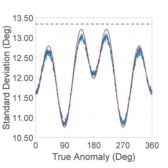
The Monte Carlo simulation and analytical approximation model are illustrated in Figure 5. Figure 5a shows exactly the same result as that in Figure 4b, which confirms Equation (45) in the analytical approximation model. The results of $\sigma \left[\mathrm{QPE}\right]$ in Figure 5b, however, are presented in a slightly complex form. This is because of the combination of the properties of $\sigma \left[{\mathrm{QPE}}_v\right]$ and $\sigma \left[{\mathrm{QPE}}_a\right]$.

The dashed magenta line in Figure 5b is $\sigma {\left[\mathrm{QPE}\right]}_{max}$. This maximum value does not equal the exact maximum of $\sigma \left[\mathrm{QPE}\right]$; instead, it has a $1.80\%$ relative error with the given simulation parameters. The most important advantage of $\sigma {\left[\mathrm{QPE}\right]}_{max}$ is that researchers can calculate this value easily with the aid of only a calculator and the appropriate parameters, combined with Equation (47) and related equations, and an acceptable approximation maximum value can still be determined.

5. Discussion

We designed an analytical approximation model of the QPE introduced by orbit determination errors. Our aim is to reduce the calculations and the processing time while revealing the core of the process by which error is transferred to QPE calculations. The technical parameter iteration period during early-stage development for an onboard real-time SAR imaging mission will benefit from the proposed methods.

SAR imaging requires the relative position, velocity, and acceleration vectors between the radar antenna and the targets to estimate the Doppler centroid and Doppler rate. Currently, in many ground-based processing systems for existing SAR missions, high-accuracy orbit determination data are applied to estimate the Doppler parameters. Such data have a time delay from the SAR raw data acquisition period, which is usually in the range of several hours or more. For real-time onboard SAR imaging missions, it is not realistic to wait for such high-accuracy orbit determination data to meet the “real-time” requirement. Real-time onboard orbit determination data have to be applied in the real-time onboard SAR imaging procedure. Current spaceborne SAR missions are usually based on a professional remote sensing satellite platform, and they are not as sensitive to perturbation. For a spaceborne SAR payload mounted on a small satellite platform to perform a constellation mission, such as MirrorSAR proposed by the DLR [27], there will be some differences (i.e., it is not as steady as a large remote sensing satellite platform) in the movement of the actual target satellite. In these situations, the errors in the real-time onboard orbit determination data should be evaluated in order to examine whether they will jeopardize the new real-time SAR imaging mission concept.

There exist other terms of phase error in the context of SAR data processing [28]. Besides QPE, there are linear, higher-order (more than cubic), sinusoidal, and random phase errors, among others. We selected QPE as the error of interest because it has defocus and loss-of-resolution effects on the image. An acceptable QPE should be seen as a tool that is used out of necessity but is not adequate for new SAR missions.

Research on the prediction of SAR imaging quality from the precision of the orbit ephemeris has been carried out [29]: the upper limit expressions of multiple phase errors and their sensitivity to the orbit ephemeris covariance have been previously established. However, this method has two major limitations when applied to spaceborne real-time SAR imaging missions. Firstly, those upper limits only reflect the extreme situation, which will not always occur during a mission. We need to examine the whole situation of the phase error, as well as its probability form. Currently, the numerical simulation method can produce the probability of the phase error, but it is time-consuming. Secondly, in spaceborne real-time SAR imaging missions, it is impossible to get the orbit ephemeris directly, and it is calculated from onboard orbit determination data. The direct link between the precision of the onboard orbit determination data and the phase error in SAR imaging is still unclear. The proposed analytical approximation model is a potential solution to the two limitations above. With the precision of the onboard orbit determination system, which can be measured on the ground, the proposed analytical approximation model gives the direct QPE probability distribution result, which can simplify the analysis.

Compared with existing methods, the proposed analytical approximation model reduces the total calculations and processing time while revealing the core of the process by which errors are transferred to QPE calculations. This proposed analytical approximation model can reveal the QPE distribution, compared with the extreme value method mentioned in Section 1. For the numerical simulation method, with M error samples for each true anomaly calculation point and a total of N true anomaly calculation points, the calculation complexity reaches $O\left(MN\right)$. It is important to point out that M is usually a large number for better statistical results. No error sample set is generated in the analytical approximation model; thus, the calculation complexity is reduced. The QPE distribution result for N true anomaly calculation points is $O\left(N\right)$, and for the distribution parameters, the validated true anomaly $\nu \in \left[0,2\pi \right]$ is $O\left(1\right)$, which can significantly reduce the total calculation and processing time. Spaceborne real-time SAR imaging mission designers can quickly determine the maximum QPE with the help of only a calculator and the appropriate parameters. Therefore, this model will accelerate the technical parameter iteration procedure during the early-stage development of an onboard real-time SAR imaging mission and provide strong proof for the feasibility of such spaceborne real-time SAR missions.

There will always be some processing blocks in the design of a spaceborne SAR system. For each processing block, the errors introduced by processing must be limited for optimal performance of the whole system. From the design practice of the existing system, an azimuth impulse response width of $1.02$ can be an acceptable limitation for a single processing block, which equals a QPE of no more than $0.27\pi$ [23]. The results in Section 4 are used here as an example. With the analytical approximation model, the result, and the three-sigma rule, it is clear that, with the simulation parameters given, if $\mathbb{E}\left[\Delta f_{r,a}\right]$ is removed during the Doppler rate calculation, then the QPE introduced by the onboard orbit determination system will be less than 40.02${}^{\circ }$, with a probability of 99.73%. This result equals an azimuth impulse response width of less than 2%, with a probability of 99.73%.

In its current form, the proposed analytical approximation model is given when the attitude error is ignored; i.e., the orbit determination error and the attitude error of the platform are decoupled. The next generation of the analytical approximation model will take the attitude error into consideration in order to examine the coupled relationship. In addition, for spaceborne bistatic real-time SAR imaging missions, a bistatic form of the model will be needed. These two directions will be our future research topics.

6. Conclusions

As the errors in the state vectors from an onboard orbit determination system for a spaceborne SAR affect real-time SAR imaging quality, this paper proposes an analytical approximation model to identify the introduction of QPE by state vector errors. This analytical approximation model can provide approximation results at two granularities, i.e., the approximation with the satellite’s true anomaly as the independent variable and the approximation for $\nu \in \left[0,2\pi \right]$. Compared with numerical simulation methods such as Monte Carlo, the proposed analytical approximation model reduces the total calculations and processing time. Another benefit of the proposed analytical approximation model is that it reveals the core of the error transfer, so each parameter’s role in the introduced QPE is clear. Spaceborne real-time SAR imaging mission designers can quickly determine QPE with the help of only a calculator and the appropriate parameters. In some ways, this will accelerate the technical parameter iteration period during early-stage development of an onboard real-time SAR imaging mission and provide convincing evidence of the feasibility of spaceborne real-time SAR missions.

References

- Moreira, A.; Brodacholl, A.; Dom, J.; Kochsiek, F.; Potzsch, W. Airborne real-time SAR processing activities at DLR. In Proceedings of the IGARSS ’92 International Geoscience and Remote Sensing Symposium, Houston, TX, USA, USA, 26–29 May 1992; Volume 1, pp. 412–414. [Google Scholar]
- Tian, H.; Chang, W.; Li, X. Integrated system of mini-SAR real-time signal processing and data storage. In Proceedings of the 2015 IEEE Radar Conference, Johannesburg, South Africa, 27–30 October 2015; pp. 354–358. [Google Scholar]
- Jia, G.; Buchroithner, M.; Chang, W.; Li, X. Simplified Real-Time Imaging Flow for High-Resolution FMCW SAR. IEEE Geosci. Remote Sens. Lett. 2015, 12, 973–977. [Google Scholar]
- Gu, C.; Chang, W.; Li, X.; Jia, G.; Liu, Z. A compact FMCW SAR real-time imaging system and its performance analysis. In Proceedings of the IET International Radar Conference, Hangzhou, China, 14–16 October 2015. [Google Scholar]
- Li, C.; Jie, L.; Cui, L.; Yao, D. The Squinted-looking SAR real-time imaging Based on Multi-core DSP. In Proceedings of the IET International Radar Conference, Hangzhou, China, 14–16 October 2015; p. 4. [Google Scholar] [CrossRef]
- Moreira, A. Real-time synthetic aperture radar (SAR) processing with a new subaperture approach. IEEE Trans. Geosci. Remote Sens. 1992, 30, 714–722. [Google Scholar] [CrossRef]
- Palm, S.; Wahlen, A.; Stanko, S.; Pohl, N.; Wellig, P.; Stilla, U. Real-time onboard processing and ground based monitoring of FMCW-SAR videos. In Proceedings of the EUSAR 2014 10th European Conference on Synthetic Aperture Radar, Berlin, Germany, 3–5 June 2014; pp. 1–4. [Google Scholar]
- Que, R.; Ponce, O.; Scheiber, R.; Reigber, A. Real-time processing of SAR images for linear and non-linear tracks. In Proceedings of the 2016 17th International Radar Symposium (IRS), Krakow, Poland, 10–12 May 2016; pp. 1–4. [Google Scholar]
- Que, R.; Ponce, O.; Baumgartner, S.V.; Scheiber, R. Multi-mode real-time SAR on-board processing. In Proceedings of the EUSAR 2016—11th European Conference on Synthetic Aperture Radar, Hamburg, Germany, 6–9 June 2016; pp. 1–6. [Google Scholar]
- Gu, C.; Chang, W.; Li, X.; Jia, G.; Luan, X. A new distortion correction method for FMCW SAR real-time imaging. IEEE Geosci. Remote Sens. Lett. 2017, 14, 429–433. [Google Scholar] [CrossRef]
- Sun, G.C.; Liu, Y.; Xing, M.; Wang, S.; Guo, L.; Yang, J. A Real-Time Imaging Algorithm Based on Sub-Aperture CS-Dechirp for GF3-SAR Data. Sensors 2018, 18, 2562. [Google Scholar] [CrossRef] [PubMed]
- Walker, B.; Sander, G.; Thompson, M.; Burns, B.; Fellerhoff, R.; Dubbert, D. A High Resolution, Four-Band SAR Testbed with Real-Time Image Formation. In Proceedings of the International Geoscience and Remote Sensing Symposium, Lincoln, NE, USA, 31–31 May 1996; Volume 3, pp. 1881–1885. [Google Scholar]
- Wang, J.; Xue, G.; Zhou, Z.; Song, Q. A new subaperture nonlinear chirp scaling algorithm for real-time UWB-SAR imaging. In Proceedings of the 2006 CIE International Conference on Radar, Shanghai, China, 16–19 October 2006; pp. 1–4. [Google Scholar]
- Malanowski, M.; Krawczyk, G.; Samczyński, P.; Kulpa, K.; Borowiec, K.; Gromek, D. Real-time high-resolution SAR processor using CUDA technology. In Proceedings of the 2013 14th International Radar Symposium (IRS), Dresden, Germany, 19–21 June 2013; Volume 2, pp. 673–678. [Google Scholar]
- Tang, H.; Li, G.; Zhang, F.; Hu, W.; Li, W. A spaceborne SAR on-board processing simulator using mobile GPU. In Proceedings of the 2016 IEEE International Geoscience and Remote Sensing Symposium (IGARSS), Beijing, China, 10–15 July 2016; pp. 1198–1201. [Google Scholar]
- Ding, Z.; Xiao, F.; Xie, Y.; Yu, W.; Yang, Z.; Chen, L.; Long, T. A Modified Fixed-Point Chirp Scaling Algorithm Based on Updating Phase Factors Regionally for Spaceborne SAR Real-Time Imaging. IEEE Trans. Geosci. Remote Sens. 2018, 56, 7436–7451. [Google Scholar] [CrossRef]
- Sugimoto, Y.; Ozawa, S.; Inaba, N. Near Real-Time SAR Image Focusing Onboard Spacecraft. In Proceedings of the IGARSS 2018—2018 IEEE International Geoscience and Remote Sensing Symposium, Valencia, Spain, 22–27 July 2018; pp. 8038–8041. [Google Scholar]
- Bergeron, A.; Doucet, M.; Harnisch, B.; Suess, M.; Marchese, L.; Bourqui, P.; Desnoyers, N.; Legros, M.; Guillot, L.; Mercier, L.; et al. Satellite on-board real-time SAR processor prototype. In Proceedings of the International Conference on Space Optics—ICSO 2010, International Society for Optics and Photonics, Rhodes Island, Greece, 4–8 October 2010; Volume 10565, p. 105652W. [Google Scholar]
- Montenbruck, O.; Yoon, Y.; Gill, E.; Garcia-Fernandez, M. Precise orbit determination for the TerraSAR-X mission. In Proceedings of the International Symposium on Space Technology and Science, Kanazawa, Japan, 4–11 June 2006; Volume 25, p. 613. [Google Scholar]
- Yu, Z.; You, Z. Real-time onboard orbit determination using GPS navigation solutions. In Proceedings of the 2011 First International Conference on Instrumentation, Measurement, Computer, Communication and Control, Beijing, China, 21–23 October 2011; pp. 949–952. [Google Scholar]
- Yang, Y.; Yue, X.; Dempster, A.G. GPS-based onboard real-time orbit determination for LEO satellites using consider Kalman filter. IEEE Trans. Aerosp. Electron. Syst. 2016, 52, 769–777. [Google Scholar] [CrossRef]
- Yan, X.; Chen, J.; Yang, W. Monte Carlo Analysis of Orbital Station Motion Parameter Errors Influence on SAR Azimuth Resolution Degradation. In Proceedings of the IGARSS 2018—2018 IEEE International Geoscience and Remote Sensing Symposium, Valencia, Spain, 22–27 July 2018; pp. 7805–7808. [Google Scholar]
- Cumming, I.; Wong, F. Digital Processing of Synthetic Aperture Radar Data: Algorithms and Implementation; Artech House Remote Sensing Library; Artech House: Norwood, MA, USA, 2005. [Google Scholar]
- Crassidis, J.; Junkins, J. Optimal Estimation of Dynamic Systems; Chapman & Hall/CRC Applied Mathematics & Nonlinear Science; CRC Press: Boca Raton, FL, USA, 2004. [Google Scholar]
- Raney, R. Doppler properties of radars in circular orbits. Int. J. Remote Sens. 1986, 7, 1153–1162. [Google Scholar] [CrossRef]
- Fiedler, H.; Boerner, E.; Mittermayer, J.; Krieger, G. Total zero Doppler steering-a new method for minimizing the Doppler centroid. IEEE Geosci. Remote Sens. Lett. 2005, 2, 141–145. [Google Scholar] [CrossRef]
- Krieger, G.; Zonno, M.; Mittermayer, J.; Moreira, A.; Huber, S.; Rodriguez-Cassola, M. MirrorSAR: A Fractionated Space Transponder Concept for the Implementation of Low-Cost Multistatic SAR Missions. In Proceedings of the EUSAR 2018 12th European Conference on Synthetic Aperture Radar, Aachen, Germany, 4–7 June 2018; pp. 1–6. [Google Scholar]
- Carrara, W.; Goodman, R.; Majewski, R. Spotlight Synthetic Aperture Radar: Signal Processing Algorithms; Artech House Remote Sensing Library; Artech House: Norwood, MA, USA, 1995. [Google Scholar]
- Jin, M.Y. Prediction of SAR focus performance using ephemeris covariance. IEEE Trans. Geosci. Remote Sens. 1993, 31, 914–920. [Google Scholar] [CrossRef]
Figure 1.
The orbital plane (OP) coordinate system and the ECI system. Elements related to the OP coordinate system are in red. is the argument of periapsis, i is the orbit eccentricity, is true anomaly, and is the center off-nadir angle in SAR.
Figure 2.
Velocity vector term: numerical simulation results (blue) and analytical approximation results (red). The figures show that the results from the analytical approximation model are consistent with the numerical simulation results. (a,b) The expected values have no significant relationship with the variation in the true anomaly and are positioned at a relatively low level, i.e., around zero. The differences between the two sets of results in (c,d) are due to the ignored terms in the approximation derivations.
Figure 3.
The true anomaly result from measurements between numerical simulation and the analytical approximation model. (a) The analytical approximation model (red) fits the numerical simulation (blue) in most areas of true anomaly. However, at certain true anomalies, which are the unique positions of the satellite in its orbit, the difference between the two sets of results increases. (b) At around and , significant peaks arise for approximately in the standard deviation of .
Figure 4.
Acceleration vector term: numerical simulation results (blue) and analytical approximation results (red). The analytical approximation results are consistent with the numerical simulation results. The expected values in (a,b) no longer have an expected value of zero, indicating different characteristics from those of the velocity vector terms. The differences around and of true anomaly between the two sets of results in (c,d) are due to the ignored terms in the calculated true anomaly approximation derivations.
Figure 5.
QPE result from numerical simulation (blue) compared with that from the analytical approximation model (red). The expected value and standard deviation of QPE are shown in (a) and (b), respectively. The dashed magenta line in (b) is the value of from Equation (47).