The Inter-Calibration of the DSCOVR EPIC Imager with Aqua-MODIS and NPP-VIIRS

Abstract

The Deep Space Climate Observatory (DSCOVR) through the earth polychromatic imaging camera (EPIC) continuously observes the illuminated disk from the Lagrange-1 point. The EPIC sensor was designed to monitor the diurnal variation of ozone, clouds, aerosols, and vegetation, especially those features that benefit from observation near-backscatter conditions. The EPIC sensor does not contain any onboard calibration systems. This study describes the inter-calibration of EPIC channels 5 (0.44 µm), 6 (0.55 µm), 7 (0.68 µm), and 10 (0.78 µm) with respect to Aqua-MODIS and NPP-VIIRS. The calibration is transferred using coincident ray-matched reflectance pairs over all-sky tropical ocean (ATO) and deep convective cloud (DCC) targets. A robust and automated image-alignment technique based on feature matching was formulated to improve the navigation quality of the EPIC images. The EPIC V02 dataset exhibits improved navigation over V01. As the visible channels display similar spatial features, a single visible channel can be used to co-register the remaining visible bands. The VIIRS-referenced EPIC ATO and DCC ray-matched calibration coefficients are within 0.3%. The EPIC four-year calibration trends based on VIIRS are within 0.15%/year. The MODIS-based EPIC calibration coefficients were compared against the Geogdzhayev and Marshak 2018 published calibration coefficients and were found to be within 1.6%.

1. Introduction

The Deep Space Climate Observatory (DSCOVR) [1] satellite was launched on 11 February 2015 and arrived at the Lagrange point 1 (L1) point on 8 June 2015. L1 is located 1.5 million km away from the Earth in the solar direction. The DSCOVR satellite, having both sun- and earth-viewing sensors, orbits the sun and has the same orbital period as the Earth. This positioning allows the earth polychromatic imaging camera (EPIC) sensor to continuously view the sunlit portion of the Earth [2].

EPIC and geostationary (GEO) full-disk images provide similar Earth views. The GEO full disk image, however, is always centered at the equator and never captures Earth’s imagery poleward of ±70° latitude. The EPIC image center varies seasonally with the Earth’s inclination because L1 is coplanar with the Earth’s orbit around the Sun. This orientation allows EPIC to view the polar region tilted towards the sun during solstice events and both poles during equinox events [2]. The orbital configuration of DSCOVR in the L1 position is such that EPIC cannot view the entire sunlit side of the Earth. As a consequence of its position, EPIC acquires the Earth-view measurements under near backscattering conditions with a scattering angle between 168.5° and 175.5°.

The EPIC sensor has four spectral bands between 0.3 µm and 0.4 µm, and six spectral bands between 0.4 µm and 0.8 µm. The channel bandwidths are all less than 3 nm. The EPIC charge-coupled device (CCD) 2-D detector array can easily image the Earth near-instantaneously, and uses a filter wheel to cycle through the spectral bands. The EPIC sensor was designed to observe the diurnal variation of clouds, ozone, vegetation, and aerosols. Some of these retrievals benefit from near-backscatter views that are not typically provided by low-Earth-orbit sensors. Unfortunately, the data link transmission rate limits the operational sampling of the Earth from 68 to 110 min depending on the season [3].

In order for the EPIC-generated retrievals to be useful for scientific analysis, the EPIC sensor is expected to be properly calibrated. The EPIC sensor does not have any onboard calibration systems and therefore is calibrated using vicarious methods. The moon can be used as a stable calibration during lunar transects. As the moon does not have an atmosphere, the oxygen absorption band and the corresponding adjacent reference band can easily be inter-calibrated by assuming the lunar reflectance is identical for both bands. Earth-based invariant target calibration can also be used as long as the Earth target is properly characterized over the observed range of EPIC view and solar angles. For EPIC, the greatest challenges for Earth invariant target calibration are achieving sufficient sampling and overcoming questionable navigation accuracy, which may be in error by 50 km [4]. The EPIC navigation is improved by employing a navigation-correction algorithm based on spatial-feature-matching with MODIS. Fortunately, a new EPIC dataset record release is expected to be available shortly following this publication, with two days of the new R06 EPIC dataset having already been made available to the science team for testing. This study compares the navigation improvement between the EPIC V01, V02, and R06, datasets.

Rather than using invariant targets, EPIC sensors are calibrated using the well-characterized MODIS and VIIRS reference instruments. Ray-matching, or bore-sighting, coincident EPIC and MODIS/VIIRS analogous spectral bands allows EPIC to be standardized to the reference calibration. Comparing the relative stability of the EPIC sensor with respect to MODIS/VIIRS may reveal possible anomalous EPIC sensor channel calibration drifts.

Two independent ray-matching calibration methods are considered for this study. The first method uses 50-km coincident MODIS/VIIRS and EPIC ray-matched radiances located over tropical oceans, and is referred to as all-sky tropical ocean ray-matching (ATO-RM). The second method uses 25-km coincident MODIS and EPIC ray-matched radiances located over deep convective clouds (DCC-RM), regardless of underlying surface type. Consistency between the two-independent ray-matching methods lends confidence to both methods. This study also compares the EPIC V02 and R06 calibration results.

This paper is a follow-on study of the Haney et al. 2106 [4] EPIC calibration methodology paper. It introduced an automated navigation-correction algorithm, formulated the spectral band adjustment factors (SBAF) critical for inter-calibration due to the very narrow EPIC spectral response functions, and evaluated the straylight improvement of V02. This paper improves upon the methodology, quantifies the navigation-correction shifts between the two EPIC versions, provides the EPIC calibration gain and trends for all channels based on a 3.5-year record with respect to both MODIS and VIIRS and notes their consistency, and compares them to the Geogdzhayev and Marshak [5] calibration gains.

The paper is outlined as follows. Section 2 (Methodology) contains the description of the EPIC, Aqua-MODIS, and NPP-VIIRS datasets. It also highlights the navigation correction, ATO-RM, and DCC-RM methodologies, the latter two of which require a SBAF to account for the EPIC and reference radiance difference due to the disparate band spectral response functions. Section 3 (Results) quantifies the EPIC V01, V02, and R06 navigation improvements. The resulting EPIC V02 and R06 ATO-RM calibration coefficient statistics are compared. The EPIC V02 mean record calibration gains based on the ATO-RM and DCC-RM are evaluated for consistency using both Aqua-MODIS and NPP-VIIRS as a reference. Similarly, the EPIC V02 record calibration temporal trends are compared against MODIS and VIIRS. Section 4 (Discussion) highlights comparisons of the EPIC ATO-RM and DCC-RM relative to the Geogdzhayev and Marshak [5] calibration gains. Lastly, Section 5 (Conclusions) summarizes the findings.

2. Methodology

2.1. Data

The NASA DSCOVR-EPIC imager L1B data V01 products were available between June 2015 and July 2017, whereas the V02 data were analyzed between June 2015 and October 2018. The main difference between V01 and V02 are the stray light and flatfielding improvements, which resulted in increasing the contrast between bright and dark pixels as well as geolocation improvements [5]. Two days (5 September 2015 and 19 April 2016) of the latest test dataset, known as version R06, was made available to the DSCOVR science team for analysis. The EPIC image is produced by the 2048 by 2048 CCD detector array [2]. The nominal L1B pixel resolution is 18 km, except for the 0.443 µm band, which retains the nominal pixel resolution of 8 km. The EPIC pixel-level L1B measurements are in photon counts per second (cnt s⁻¹), which are proportional to radiance. EPIC has a quantization rate of 12 bits. EPIC uses a filter wheel to cycle through the 10 reflected solar band (RSB) channels, which takes approximately 7 min, during which the Earth rotates ~200 km at the equator. All 10 bands are geo-rectified onto the same common EPIC projection grid by applying a complex spherical geometry geolocation algorithm based on star tracking, an optical path model, satellite ephemeris, and the location of the Earth disk on the CCD array [3].

Aqua-MODIS Collection 6.1 (C6.1) L1B 1-km nominal pixel resolution radiances were used. The SNPP VIIRS V1 L1B dataset generated by the NASA Land Science Investigator-led Processing System (SIPS) provided stable calibration during the EPIC observation period. VIIRS has both imager (I) and moderate (M) resolution bands. The I and M channels have 375-m and 750-m nominal pixel resolutions, respectively. Furthermore, VIIRS uses pixel aggregation in order to maintain the pixel resolution across the scan. For convenience, this study used the Clouds and the Earth’s Radiant Energy System (CERES) project locally archived MODIS and VIIRS datasets, where the MODIS pixel-level data was subsampled at 2-km resolution, and both the VIIRS I and M bands were sub-sampled at 1.5 km. Finally, Aqua and NPP are in a sun-synchronous orbit with a local equator crossing time of 01:30 PM.

The following EPIC, MODIS, and VIIRS band nomenclature is used in this paper. EPIC bands 5 through 10 are identified as E5 through E10. The Aqua-MODIS bands are designated as A bands and the NPP-VIIRS M and I bands are referred as such.

Both MODIS and VIIRS rely on solar diffusers to transfer the ground-characterized reference on orbit. Once in orbit, the solar diffusers and lunar looks are used to stabilize the calibration. The MODIS/VIIRS measurements are reflectance based, that is, the at sensor radiance is scaled by the solar diffuser radiance. The EPIC sensor does not have an onboard calibration reference and the observations are proportional to radiance units (cnt s⁻¹). The EPIC radiance (Rad_EPIC) is proportional to the MODIS (or VIIRS) L1B reflectance (Ref_MODIS):

$$Re{f}_{MODIS}=\frac{Ra{d}_{MODIS}\times d^2}{E_{SUN}} \propto Ra{d}_{EPIC}$$

(1)

where E_SUN is the band solar constant in radiance units and d is the Earth-Sun distance in astronomical units. The L1B reflectance or scaled radiance is not be confused with the true reflectance (Ref_TRUE):

$$Re{f}_{TRUE}=\frac{Rad \times d^2}{E_{SUN} \times \cos \left(SZA\right)}$$

(2)

The MODIS L1B reflectance is defined as the true reflectance multiplied by the cosine of the solar zenith angle cos(SZA), which equals the measurement MODIS reflectance [6]. The NASA Land SIPS VIIRS L1B reflectance is defined exactly as the MODIS L1B reflectance [7]. The MODIS L1B radiance is computed by multiplying the L1B reflectance by the MCST solar spectra-based band solar constant [8], and the NPP-VIIRS L1B radiances are computed using the IDPS (MODTRAN 4.3) solar spectra [9]. The band solar constants (E_SUN) in Wm⁻²sr⁻¹µm⁻¹ units can be computed using the NASA Langley solar constant tool [10]. When comparing the MODIS and VIIRS based EPIC radiance calibration gains, it must be noted that part of the difference is due to the band solar constant difference. For example, the A1 and M5 band solar constant difference exceeds 4%. The MODIS/VIIRS and EPIC reflectance difference owed to the spectral band disparity still are expected to be accounted for, however (see Section 2.6).

2.2. EPIC Navigation

The ray-matching calibration algorithm requires coincident and angle-matched EPIC and MODIS radiance pairs. The EPIC nominal field of view (FOV) is 18 km. Whereas, the MODIS pixels had a 1-km nominal resolution, but were sub-sampled at 2 km. Two spatial matching approaches can be utilized given the relatively large difference between the MODIS/VIIRS and EPIC FOVs. The first approach maps the MODIS/VIIRS high-resolution pixels into the larger EPIC FOV. The second approach simply averages EPIC and reference pixel radiances onto the same spatial grid.

The first approach has been regularly employed over the decades, starting with mapping the Geostationary Operational Environmental Satellite (GOES)-2 1-km pixels to the Nimbus-7 Earth Radiation Budget (ERB) scanner 90-km FOV [11]. However, more recently, as part of the Global Space-based Inter-calibration System (GSICS) effort, GEO ~4-km IR pixel-level radiances were averaged within the larger infrared atmospheric sounding interferometer (IASI) 12-km FOV for the purpose of establishing a calibration standard [12]. For oblique views, the pixel geometry is more elliptical, and as such the pixel radiances are weighted using a geometric point spread function in order to mitigate the spatial matching errors [13]. To determine the GOES-16 geolocation accuracy with respect to the NPP-VIIRS navigation reference, the reference images are shifted at the sub-pixel resolution and mapped into the GOES-16 FOV using a 2-dimensional FFT algorithm [14].

The second approach is usually implemented when given two high-resolution datasets whose pixel centers are not aligned. For example, the well-calibrated Tropical Rainfall Measuring Mission (TRMM), visible and infrared scanner (VIRS) (nominal 2 km), and European Remote-sensing Satellite (ERS)-2 Along-Track Scanning Radiometer (ATSR)-2 (1 km) sensors were used to calibrate the GOES-8 (1 km) visible channel radiances using either a 0.5° or 0.25° latitude by longitude grids [15]. Further, GOES-8 (1 km) and Meteosat-7 (2.5 km) visible imager pixel radiances were averaged onto a 0.06° grid in order to inter-calibrate the two GEO imagers [16]. Similarly, the Meteosat-9 (3 km) visible imager was intercalibrated with NOAA17/18-Advanced Very High Resolution Radiometer (AVHRR) (3 × 5 km), and Terra/Aqua-MODIS (1 km) using a 0.15° latitude by 0.15° longitude grid [17]. The GSICS visible ray-matching algorithm uses a 0.5° latitude by 0.5° longitude grid to intercalibrate GEO sensors against MODIS or VIIRS [18]. The advantage of increasing the spatial grid size is mitigated effects of cloud advection, navigation error, and parallax error, thereby reducing the uncertainty of inter-calibration coefficients [19].

Whenever there is a large FOV difference, the first approach is preferred, however, the first approach is not used in this study because the EPIC V02 projection requires the navigation improvement. The second approach can easily be implemented to correct the EPIC navigation. The underlying grid resolution dictates the navigation accuracy. The navigation correction algorithm has been documented in [4] and is briefly summarized here. For each EPIC image acquired, any MODIS/VIIRS granules that are located within ±30° latitude and within 15 min of an EPIC image time are paired. A 0.25° latitude by 0.25° longitude grid is used, which is slightly larger than the EPIC nominal FOV, to ensure that each grid point contains an EPIC pixel observation. The EPIC point spread function was not considered in the gridding process. The point spread function is a combination of the optics and the rotation of the Earth. By applying the point spread function in a future study may decrease the uncertainty in both the navigation correction and resulting calibration gains.

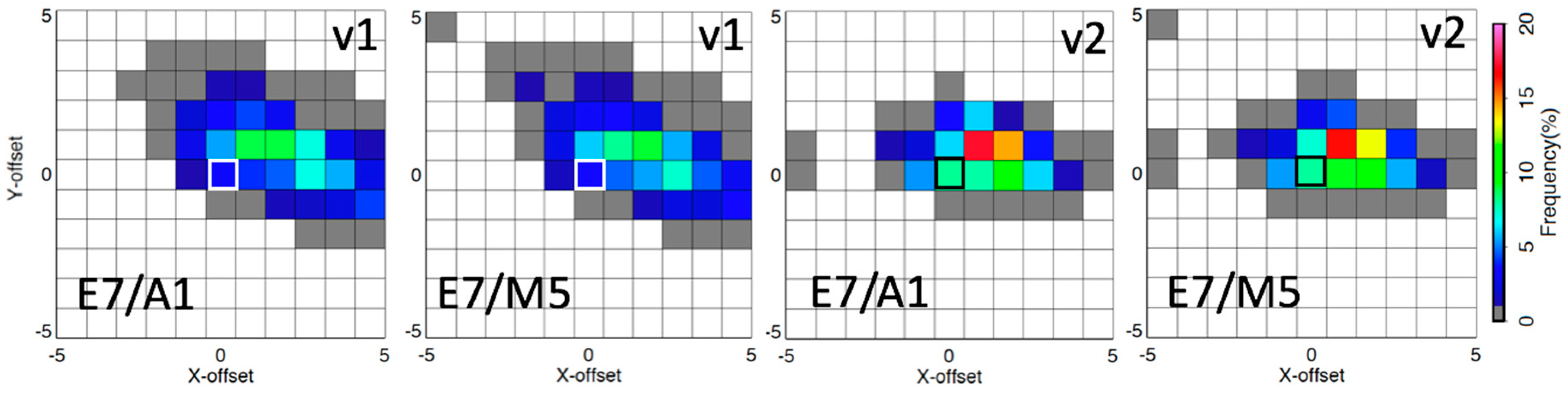
For each image pair, the EPIC gridded radiances are allowed to shift by 5 grid locations in both the latitude and longitude direction with respect to the reference grid. Notably, neither perfect ray-matching nor spectral correction is required for navigation analysis. The EPIC and MODIS/VIIRS radiance pairs are linearly regressed and the square of the correlation coefficient (r²) is noted. The EPIC image shift with the greatest r² determines the EPIC navigation correction. The EPIC and MODIS/VIIRS matched grids are then used by the ray-matching calibration algorithms. There may be several reference granules that overlay a single EPIC image, and each MODIS/VIIRS granule is matched independently to each EPIC band.

2.3. ATO-RM

All-sky tropical ocean (ATO) targets provide near-overhead sun observations that cover the entire reflectance dynamic range and utilizes most of the images contained in the EPIC record. The all-sky tropical ocean ray-matching (ATO-RM) algorithm follows the historical approach of [15,18]. Both the EPIC and MODIS 0.25° gridded reflectance values are first averaged into a 0.5° gridded domain. The coincident (within 15 min) reflectance pairs are then ray-matched within 15° in both view zenith angle (VZA) and relative azimuthal angle (RAA). Any grid region containing more than 10% land is excluded because land spectra are geographically and temporally varying. Sun-glint conditions are also avoided. Lastly, a spatial homogeneity threshold is applied to eliminate spectrally complex, partly cloudy conditions, wherein the standard deviation of the eight surrounding and center grid reflectance is expected to be less than 20% of the average. For the E5 and E6 bands, the spatial homogeneity is set to 10%. The MODIS/VIIRS scaled radiances are normalized to the solar conditions of the EPIC measurements by multiplying by the ratio of the cosine of the solar zenith angle. The spectral band reflectance difference is considered by applying an SBAF to the MODIS/VIIRS reflectance (see Section 2.6).

Reflectance-incremented, or graduated angle matching (GAM), thresholds are applied to take advantage of uneven sampling distribution over the reflectance dynamic range [20]. Dark reflectance pairs are more numerous than bright reflectance pairs, with the low values being highly anisotropic, and brighter reflectance values more Lambertian. For the bottom quarter of the reflectance range, both the EPIC and MODIS VZA and RAA differences are restricted to 5°, but for the 2^nd quartile the VZA and RAA differences are limited to 10°. The remaining top half of the reflectance samples are matched within the initial 15° VZA and RAA difference threshold.

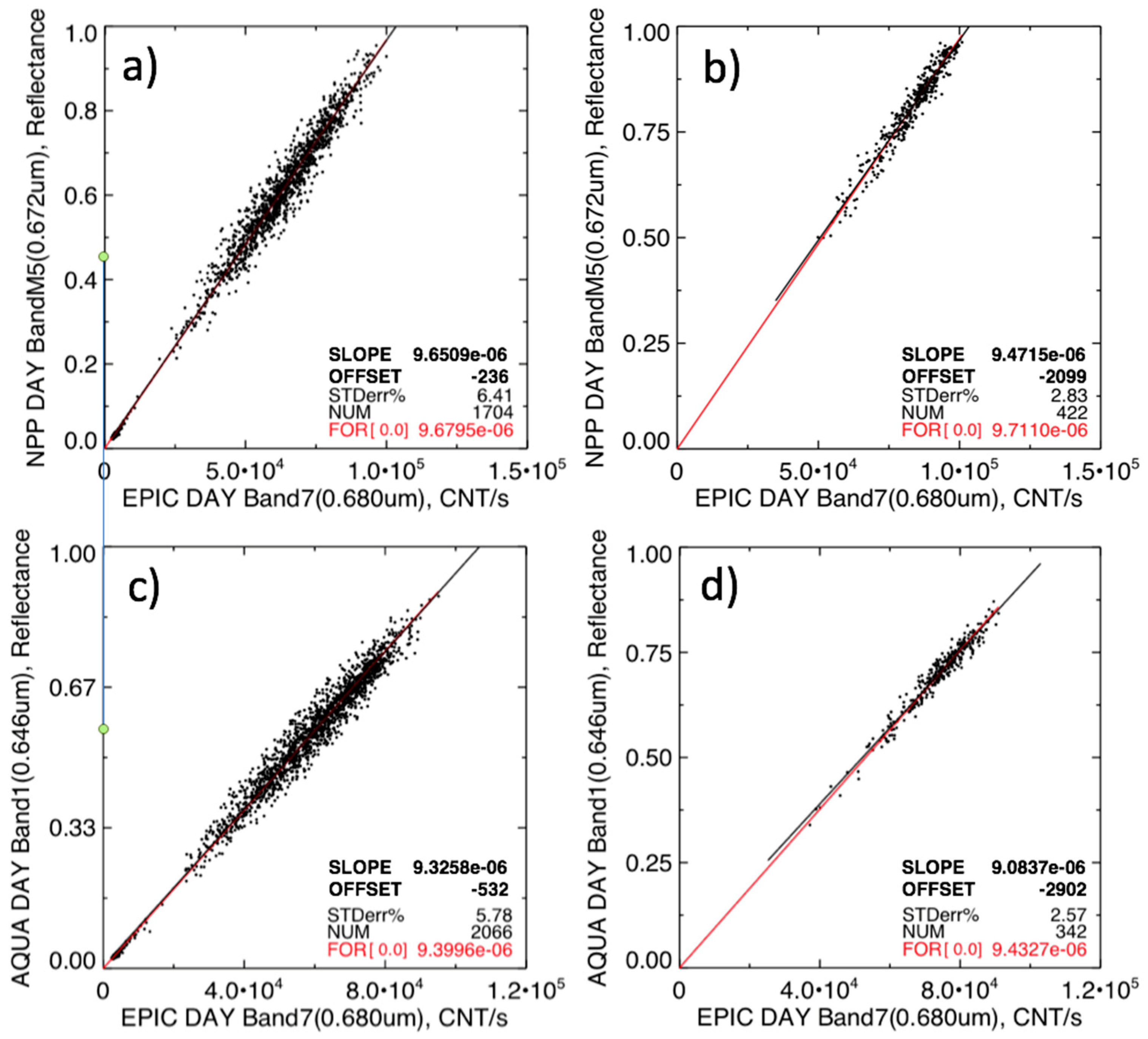
Figure 1 shows the coincident ray-matched ATO E7/M5 and E7/A1 measurement pairs observed during November 2016. It is noted how the strict angle matching of the first quartile reflectance pairs results in a narrow cluster of points along the regression line beginning near the origin. The E7/M5 and E7/A1 standard error of the linear regression is 6.4% and 5.8%, respectively. The ATO-RM reflectance, or scaled radiance, pairs show that the EPIC sensor response is linear across the dynamic range. The EPIC deep space look radiance value is assumed to be stable and properly removed. Therefore, the EPIC calibration gain is based on the linear regression through the origin and is referred to as the force fit. The standard linear regression slope and offset are also provided in Figure 1. The E7/M5 and E7/A1 slope is within 0.3% and 0.8% of the force fit, and the offset of −236 and −532, respectively, which is relatively close to 0, given the range of possible cnt s⁻¹. By specifying the offset in this way, a more accurate gain is computed and the reflectance values near the offset are improved [21].

2.4. DCC-RM

Tropical DCC are the brightest Earth targets that provide near-Lambertian reflectance for near-nadir viewing and solar illumination conditions [22]. As their cloud tops are located at the tropopause, the impact of the near infrared water vapor absorption is minimal resulting in near uniform top of atmosphere spectra for wavelengths less than 1 µm. Deep convective clouds allow for large angular matching tolerances and are associated with small SBAF uncertainties, but unfortunately are not stationary nor strictly consistent in location/time. At any given time ~0.5% of the tropics is covered by DCC [23]. The 15-min coincident EPIC and MODIS/VIIRS 0.25° grids are used to obtain the DCC-RM reflectance pairs. Potential DCC targets are identified by finding the MODIS B31 or VIIRS M15 (11 µm) grid brightness temperature (BT) that are less than 220 K. Generally, the more pristine DCC are identified with a BT less than 205 K. However, the BT threshold was increased to expand the spatial coverage in order to ensure sufficient sampling of ray-matched pairs. The identified DCC locations are then angle matched within 15° in VZA and RAA. Also, both the EPIC and MODIS/VIIRS VZA and SZA are expected to be less than 40°, and the RAA is expected to be between 10° and 170°. To avoid cloud shadowing or edge effects, the BT and visible spatial homogeneity are expected to be within 2.5 K BT and 5% of the mean value, respectively. For DCC ray-matching all surface types are utilized. The DCC reflectance may vary over land and ocean surfaces due to the cloud microphysics. This fact does not impact the DCC ray-matching results, as long as each ray-matched pair observes the same Earth viewed footprint. As with ATO-RM, the MODIS/VIIRS scaled radiance is normalized to the solar geometry of the EPIC measurement and spectrally adjusted to match the EPIC spectral band response.

Figure 1b shows the DCC-RM E7/M5 and E7/1A1 measurement pairs observed during November 2016. The E7/M5 DCC-RM force fit gain (9.7110e-6/cnt s⁻¹) is within 0.33% of the ATO-RM force fit gain (9.6795e-6/cnt s⁻¹). Similarly, the E7/A1 DCC-RM and ATO-RM force fit gains are within 0.35%. The gain consistency between ray-matching methods provides confidence that the derived gain has accurately transferred the VIIRS calibration reference. Each method has associated strengths and weaknesses. The E7/M5 and E7/1A1 DCC-RM linear regression standard error is 2.8% and 2.6%, which is less than half of the ATO-RM standard error of 6.4% and 5.8%, respectively. The SBAF uncertainty is less than 0.3% for both DCC and ATO. The DCC angular matching uncertainties are smaller than ATO-RM because DCC targets are near-Lambertian. The impact of the residual EPIC navigation and time mismatch error is greater for the DCC 0.25° grid than the ATO 0.5° grid. This impact is mitigated by applying a spatial uniformity filter of 5% for DCC-RM, which is much lower than the 20% applied for ATO-RM.

2.5. The EPIC Calibration Coefficients

The ATO-RM and DCC-RM force fit linear regression gain is used to compute the calibration coefficients based on the assumption that the EPIC calibration team has succesfully removed residual or deep space count in the L1B product. The EPIC calibration gain based on the MODIS (or VIIRS) L1B reflectance (Ref_MODIS) is computed from the EPIC cnt s⁻¹ (C_EPIC) as follows:

Ref_MODIS = gain × C_EPIC

(3)

The monthly EPIC channel gains are monitored over time to determine if the EPIC sensor is degrading. The EPIC degradation is estimated to be linear over time and is tracked as a function of the days since EPIC launch (dsl),

gain = g₀ + g₁ × dsl

(4)

where g₀ and g₁ are the linear regression coefficients. The E7/M5 ATO-RM and DCC-RM temporal gain trends are shown in Figure 2. The monthly gain noise relative to the linear regression is assumed to be associated with the uncertainty of the ray-matching calibration method and is not sensor-related. The mean record ATO-RM and DCC-RM E7 gain difference is within 0.3%. There is an insignificant negative E7 calibration drift of −0.02%/year and −0.01%/year based on the ATO-RM and DCC-RM calibration methods, respectively.

2.6. SBAF

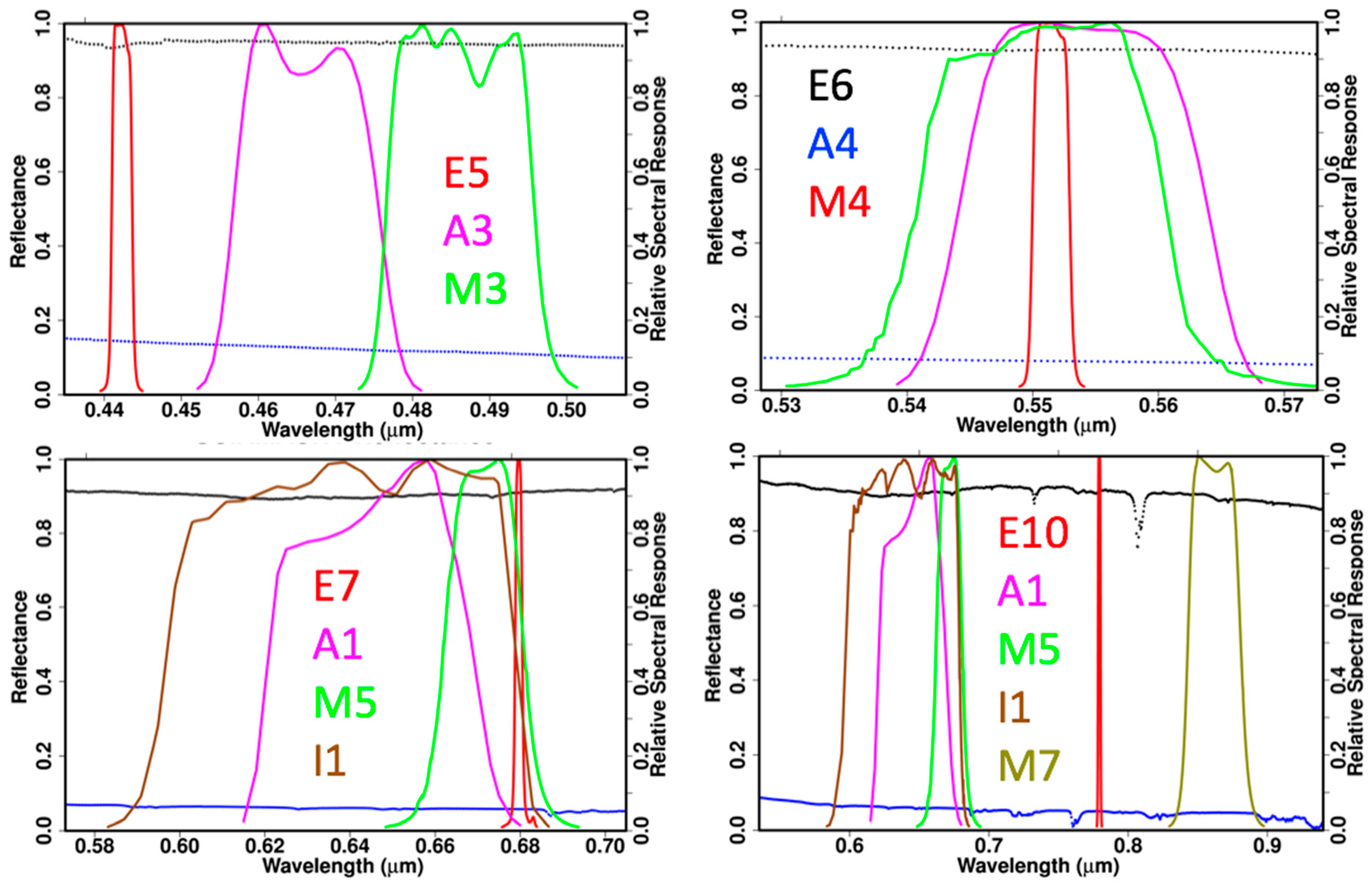
When the EPIC and MODIS/VIIRS coincident ray-matched radiance pairs are compared, the non-shared band spectral response radiance contribution is removed in order to not bias the true EPIC and MODIS/VIIRS calibration difference. The spectral band adjustment factor, or SBAF, adjusts the reference reflectance to spectrally match the EPIC channel reflectance. The Earth-reflected spectrum is the combined effect of the incoming solar spectra modified by the ground and cloud top reflection as well as the atmospheric absorption. The Envisat SCanning Imaging Absorption SpectroMeter for Atmospheric CHartographY (SCIAMACHY) hyper-spectral visible radiances are used to estimate the SBAF for all of the MODIS/VIIRS and EPIC band pairs shown in Figure 3. The 2002 to 2012 SCIAMACHY hyper-spectral record does not overlap the EPIC record, but SCIAMACHY footprints with similar viewing and solar geometry found for EPIC and MODIS/VIIRS ATO and DCC ray-matching conditions are used. The SCIAMACHY footprint spectra are convolved with both the EPIC and MODIS/VIIRS band spectral response functions to compute the pseudo EPIC and reference reflectance pairs. It is noted that the SCIAMACHY DCC reflectance is nearly flat across the 4 EPIC channels, except for the oxygen absorption lines in Figure 3.

All channel pair SBAFs used in this study were obtained from the NASA-Langley SBAF web tool [24,25,26]. The DCC SBAF is based on the force fit regression applied to the SCIAMACHY DCC pseudo reflectance pairs. ATO is a multi-scene target, which combines clear-ocean, partly cloudy, and bright cloud conditions. Each scene condition has a unique SBAF. A quadratic fit is applied to the pseudo reflectance pairs and predicts the SBAF along the reflectance dynamic range. The quadratic fit significantly lowers the standard error of the ATO pseudo reflectance pairs from a linear fit, in this case.

3. Results

3.1. V01 and V02 Navigation Assessment

The EPIC V01 and V02 navigation improvement was quantified by the magnitude of the shift position required to align the EPIC image with respect to the MODIS image. The EPIC shift position with the greatest r² is saved for all of the EPIC MODIS coincident image pairs. Image shifting occasionally does not return the true navigation error. For example, it is difficult to properly align images with no spatial contrast, that is having no cloud edges or coastlines. Furthermore, the greater the MODIS and EPIC viewing and solar angular differences, the greater the bidirectional effects, which may interfere with the image shifting. To help visualize the navigation correction, the navigation shift position frequency plots of the 0.25° longitude (x-axis, east is positive) by 0.25° latitude (y-axis, north is positive) EPIC V01 and V02 E7/A1 and E7/M5 band pairs are shown in Figure 4. The navigation shift position frequency results were similar for E7/A1 and E7/M5 for EPIC version 01. The MODIS and VIIRS referenced pixel navigation error was found to be nearly identical. The EPIC V01 navigation shift position was systematically biased mostly towards the northeast quadrant and was spread out across 4 grid boxes. For EPIC V02, the magnitude of the navigation shift position has been reduced and the shift was mostly concentrated within 2 grid boxes or ~50 km towards the northeast. In order to quantify the V01 to V02 E7/M5 improvement, the mean navigation-correction shift was computed based on all image pairs. The V01 east-west and north-south shifts were 43.2 ± 47.3 km and 19.1 ± 21.2 km, respectively, whereas the corresponding V02 shifts were only 27.4 ± 35.9 km and 15.9 ± 19.9 km, respectively. The V02 east-west and north-south shifts were reduced by 35% and 15%, respectively, compared with V01.

The EPIC navigation correction method works best for overlapping MODIS/VIIRS and EPIC spectral band pairings. The question of how well the navigation correction method works for the EPIC E10 bands (0.78 µm), which is paired with both the M5 (0.65 µm) and M7 (0.86 µm) bands, remains, however. It is expected that all EPIC channel image navigation is consistent because the EPIC L1B dataset was geo-rectified to a common grid. Any changes in the channel-specific navigation correction may indicate that the spectral features are not spatially consistent. Figure 5 shows that the E10/M5 and E10/M7 navigation correction is very similar to the E7/M5 or E7/A1 distributions, as in Figure 4, for both EPIC V01 and V02. The EPIC navigation correction algorithm was also tested for the EPIC oxygen absorption band E9 (0.764 µm) against the VIIRS M5 and M7 bands and the frequency distribution as shown in Figure 5. The E9 navigation error was very similar to E10, the reference band for E9. The oxygen absorption spectral band images provide enough high cloud features for image alignment. In fact, all EPIC E5 though E10 channels showed the same navigation shift position distribution (not shown). In summary, for wavelengths less than 1 µm, any reference band can be used to correct the navigation of another band.

In order to quantify the image quality improvement between the EPIC versions, EPIC V01 and V02 record mean r², of the most aligned EPIC image for each band combination is compared. The average band pair r² was 0.85 and 0.78 for V02, when pairing the E10 (0.78 µm) with the 0.86 µm and the 0.65 µm channel indicating that the E10 band (0.78 µm) was more spectrally consistent with the 0.86 µm band. The average r² of all the EPIC/MODIS band combinations as shown in Figure 3 was 0.790 ± 0.027 for V01 and 0.818 ± 0.030 for V02. For EPIC/VIIRS the r² was 0.777 ± 0.029 for V01 and 0.814 ± 0.0328 for V02. V02 showed a slight r² increase of ~0.03 across all band combinations over V01, indicating that the V02 image quality has improved over V01. It was also found that the E10 band (0.78 µm) was more spectrally consistent with the 0.86 µm band than with the 0.65 µm, because the average band pair r² was 0.85 and 0.78 for V02 for the 0.86 µm and 0.65 µm bands, respectively.

3.2. R06 Navigation Assessment

Two test days (5 September 2015 and 19 April 2016) of EPIC version (R06) were made available to the science team for evaluation. It was mentioned that the R06 navigation accuracy was significantly increased. Sufficient sampling was available for 19 April 2016, which used the ATO-RM thresholds as described in Section 2.3. The V02 and after navigation correction (V02-NAV), along with the R06 results, were compared against the NPP-I1 ATO-RM radiance pairs and displayed in Figure 6. By correcting the EPIC V02 navigation, the linear regression standard error (stderr) was reduced from 9.68% to 2.65%, which was very close to the R06 stderr of 2.39%. This result indicates that the navigation correction performed in this study is close to the R06 navigation quality. Also, the V02-NAV linear regression computed offset of 189 cnts⁻¹ was closer to the R06 value of 43 cnts⁻¹ than the V02 offset of −514 cnts⁻¹. The V02 and V02-NAV linear regression slopes were within 0.9% and 0.2% with respect to R06. However, the V02 and V02-NAV force fit gain difference was less than 0.1% when compared with R06, indicating that the force fit was more robust to compute the calibration gain than the linear regression slope.

3.3. R06 Calibration Assessment

All of the EPIC bands were compared with their VIIRS band counterparts. The band pair stderr and offset are found in

Table 1. A comparison of the EPIC E7 V02, V02 with navigation correction (V02-NAV), and R06 and NPP-VIIRS I1 (0.65 µm) band pair linear regression standard error offset for 19 April 2016.

	Standard Error (%)			Offset (cnt s−1)
Band Pair	V02	V02 NAV	R06	V02	V02 NAV	R06
E5/M3	6.92	2.65	0.99	2943	2573	2489
E6/M4	6.55	2.22	1.26	672	557	402
E7/I1	9.69	2.65	2.39	−514	189	43
E7/M5	9.63	2.67	2.38	−344	500	359
E10/I1	11.06	3.18	2.61	−942	−147	−228
E10/M5	10.96	3.22	2.68	−795	19	−10
E10/M7	10.56	2.96	2.59	−544	624	477

. On average, the band pair V02, V02-NAV, and R06 stderr were 9.34%, 2.79% and 2.13%, respectively. The EPIC navigation correction reduced the stderr by a third, and nearly reduced the stderr to the R06 baseline. The mean pair V02, V02-NAV, and R06 offset was −544 cnts⁻¹, 616 cnts⁻¹, and 505 cnts⁻¹, respectively. Note that the EPIC navigation correction reduced the offset with respect to R06 by an order of magnitude, and the V02-NAV was within ~100 cnts⁻¹ of R06.

The EPIC V02-NAV and R06 force fit calibration gains were compared. All of the band pair force fits and offset differences were within 0.3% and 500 cnt s⁻¹, respectively, except that for E5/M3. E5/M3 force fit difference was 0.8% and the offset was 2489 cnt s⁻¹ (Table 1). This result suggests that the V02-NAV and R06 calibration coefficients are similar. The offset is a good indicator of the stray light impact. Geogdzhayev and Marshak [5] noted that the impact of stray-light can be quantified by how close the offset value is to zero. The large E5/M3 offset compared with the other EPIC/VIIRS channel pairs in Table 1 is similar to the E5/A3 large offset when compared with other MODIS band pair plots displayed in Figure 4 in [5] and more than likely the effect of stray light. Most of the EPIC band R06 offsets were closer to zero than V02 suggesting that the EPIC R06 dataset reduced the impact of stray light compared with V02.

3.4. EPIC Calibration Gains

The ATO-RM and DCC-RM techniques both independently transfer the MODIS on-orbit reference calibration to the EPIC imager.

Table 2. The DCC-RM and ATO-RM EPIC V02 with MODIS and VIIRS band pair August 2015 to October 2018 mean reflectance gain (1/cnt s⁻¹) and associated trend standard error (σ) in percent, along with ATO minus DCC gain difference computed as 100%*(1-ATO-RM/DCC-RM).

	MODIS Gains						VIIRS Gains
Band Pair	DCC-RM gain	σ	ATO-RM gain	σ	ATO-DCC	Band Pair	DCC-RM gain	σ	ATO-RM gain	σ	ATO-DCC
E5/A3	8.215e-6	0.8	8.229e-6	0.5	+0.2	E5/M3	8.515e-6	0.8	8.491e-6	0.5	−0.3
E6/A4	6.612e-6	0.9	6.640e-6	0.5	+0.4	E6/M4	6.834e-6	1.0	6.829e-6	0.6	−0.0
E7/A1	9.348e-6	0.9	9.448e-6	0.7	+1.1	E7/I1	9.560e-6	1.0	9.562e-6	0.8	+0.0
						E7/M5	9.684e-6	0.9	9.709e-6	0.7	+0.3
E10/A1	1.415e-5	1.2	1.433e-5	0.9	+1.3	E10/I1	1.453e-5	1.2	1.449e-5	1.1	−0.3
						E10/M5	1.473e-5	1.2	1.472e-5	1.0	−0.1
						E10/M7	1.494e-5	1.2	1.499e-5	0.9	+0.3

provides the EPIC V02 DCC-RM and ATO-RM calibration record mean gains in reflectance units referenced to both MODIS and VIIRS between August 2015 and October 2018. Table 2 also contains the monthly gain linear regression standard error. The ATO-RM and DCC-RM gain difference in percent is also listed. The ATO-RM and DCC-RM gain differences for the EPIC and MODIS band pairs were within 1.3%. Remarkably, the VIIRS-referenced ATO-RM/DCC-RM calibration gains were within for 0.3% for all band pairs. Both the Aqua- and VIIRS-based trend standard errors were greater for DCC-RM than ATO-RM, and increased by band wavelength. For VIIRS, the ATO-RM and DCC-RM gain difference was within the DCC-RM or ATO-RM trend standard errors.

3.5. EPIC Calibration Trends

The EPIC L1B data has not been calibrated, so the degradation observed would be the true on-orbit EPIC sensor calibration drift. It is expected that the EPIC sensor degradation to be identical whether compared to either MODIS or VIIRS. The EPIC UV channels (<4 µm) degraded, on average, at 1.6% per year [3].

Table 3. The DCC-RM (DCC) and ATO-RM (ATO) EPIC V02 with MODIS and VIIRS band pair reflectance gain trend during August 2015 to October 2018. RVS is the left side scan position calibration trend difference relative to nadir. The DCC-adj and ATO-adj are the ATO-RM and DCC-RM trends with the RVS trend subtracted revealing the true EPIC sensor trend. All trend units in %/year.

	MODIS-Based Trends						VIIRS-Based Trends
Band Pair	DCC	AΤO	MODIS RVS	DCC adj	ATO adj	Band Pair	DCC	AΤO	VIIRS RVS	DCC adj	ATO adj
E5/A3	0.30	0.55	+0.30	+0.00	+0.25	E5/M3	0.39	0.42	+0.30	0.09	+0.12
E6/A4	0.53	0.72	+0.40	+0.13	+0.32	E6/M4	0.25	0.26	+0.17	0.08	+0.09
E7/A1	0.27	0.43	+0.31	−0.04	+0.12	E7/I1	0.03	0.00	+0.08	−0.05	−0.08
						E7/M5	0.01	−0.02	+0.05	−0.04	−0.07
E10/A1	0.31	0.34	+0.31	+0.00	+0.03	E10/I1	−0.06	−0.02	+0.08	−0.14	−0.10
						E10/M5	−0.07	−0.04	+0.05	−0.12	−0.09
						E10/M7	−0.12	−0.10	+0.04	−0.16	−0.14

reveals that for VIIRS the ATO-RM and DCC-RM trends are very consistent. For MODIS, however, the ATO-RM and DCC-RM trends differed up to 0.25%/year. Further, the MODIS- and VIIRS-based EPIC band trends differed, possibly because the MODIS and VIIRS L1B instrument calibration drifts had not been fully accounted for during the operational calibration process.

MODIS is a scanning radiometer that has a scan-angle dependent calibration. In C6.1 L1B product, the MODIS sensor’s response versus scan-angle (RVS) is operationally characterized using onboard calibrator measurements supplemented with the long-term instrument response derived at different scan angles over multiple pseudo-invariant calibration sites [27]. A recent study performed by Bhatt et al. [28] reported residual RVS dependencies in MODIS C6.1 calibration. The Aqua-MODIS band 1 showed a temporal positive trend of ~1.5% in its left-side scans Earth-view measurements during 2015–2018. The EPIC sensor views the Earth under backscatter conditions, and the corresponding matches from Aqua-MODIS and VIIRS are only obtained from the left side of the scan. The Aqua-MODIS trend for left-side scan positions was determined for most channels to be 0.3%/year (see MODIS RVS in Table 3). Similarly, the VIIRS-relative backscatter trend was computed for the same scan positions and was found to be insignificant, except for the two shortest wavelength bands.

The true EPIC calibration trends based on MODIS or VIIRS reference are those with the MODIS or VIIRS relative backscatter trend removed. The VIIRS-based true EPIC band trends were mostly found to be within ±0.1%/year, indicating that the EPIC sensor had not changed significantly over time. The MODIS-based DCC-RM and ATO-RM E7 and E10 trends were less than 0.1%/year. The MODIS-based ATO-RM E5 and E7 0.3%/year trends are the outliers. It is more than likely, for those bands that the simple MODIS relative backscatter trend was not adequate enough to describe the true ATO-RM or DCC-RM RVS sampling pattern.

4. Discussion

The EPIC calibration trends and gain coefficients found in this study are compared with those of Geogdzhayev and Marshak [5]. Their study employed two independent calibration methods and are briefly described here. They matched 50-km MODIS C6 and EPIC radiance pairs within 10 min and the scattering angle within 0.5°. The first method used all tropical Earth scene conditions that had a uniform radiance within 1% across a 250-km diameter. By linearly regressing all of the EPIC cnt s⁻¹ and MODIS reflectance pairs during June 2015 and March 2017, a single calibration gain was determined for the EPIC record. The second method simply averaged all EPIC pixel radiances and corresponding MODIS reflectance values that exceeded 0.6 in order to obtain the calibration gain (0.6 ref). The seasonal variation of the 0.6 ref gain over the record indicated no discernable trend, which is consistent with our study, in which the EPIC trends were mostly within 0.1%/year (see Section 3.5). The linear regression calibration gain (linear) and the 0.6 ref gain relative to the linear gain is listed in

Table 4. The June 2015 and March 2017 EPIC V02 linear regression gain (GM linear), the 0.6 reflectance gain (0.6 ref) relative to the GM linear gain in %, and the seasonal 0.6 ref gain standard deviation (GM σ) in % obtained from Geogdzhayev and Marshak [5] (their Table 2, Figure 8, and Section 6, respectively). The August 2015 to October 2018 MODIS and VIIRS band pair ATO-RM and DCC-RM based reflectance gains in % relative to the GM linear gain.

GM				MODIS			VIIRS
Band Pair	linear	0.6 ref	σ	Band Pair	DCC-GM	ATO-GM	Band Pair	DCC-GM	ATO-GM
E5/A3	8.34e-6	+0.1	0.9	E5/A3	−1.5	−1.3	E5/M3	+2.1	+1.8
E6/A4	6.66e-6	0.0	0.6	E6/A4	−0.7	−0.3	E6/M4	+2.6	+2.5
E7/A1	9.30e-5	+0.4	0.4	E7/A1	+0.0	+1.1	E7/I1	+2.8	+2.8
							E7/M5	+4.1	+4.4
E10/A2	1.435e-5	−1.7	0.6	E10/A1	−1.4	−0.1	E10/I1	+1.3	+1.0
							E10/M5	+2.6	+2.6
							E10/M7	+4.1	+4.5

, as well as the 0.6 ref gain seasonal temporal standard error. Geogdzhayev and Marshak [5] intercalibrated the E10/A2 band pair, whereas our study avoided using the A2 band given that it saturates over DCC.

Table 4 contains the DCC-RM and ATO-RM relative gains with respect to the linear gain. The MODIS DCC-RM and ATO-RM gains were within 1.5% and the 0.6 ref gain was within 1.7% of the linear gain. The Geogdzhayev and Marshak [5] calibration gains were found to be consistent with the MODIS ATO-RM and DCC-RM gains.

The EPIC gains based on the NPP-VIIRS calibration reference are also shown in Table 4. No attempt was made to radiometrically scale NPP-VIIRS to Aqua-MODIS. The VIIRS 0.65-µm I1 and M5 bands were expected to have the same calibration gains, because they share the same optical path. However, the I1 and M5 ATO-RM or DCC-RM calibration gain difference with respect to the E7 or E10 band was 1.3% and 1.6%, respectively. The I1 and M5 band gain difference was consistent with the 1.7% found in Uprety et al. [29] and that the M7 calibration was 2% larger than the I2 band. After adjusting the VIIRS M5 and M7 calibrations to resemble their corresponding I bands, all of the EPIC/VIIRS band combinations were between 1% and 3% greater than the EPIC/MODIS gains. The NASA VIIRS calibration support team (VCST) also compared the MODIS and VIIRS calibration and found a +1% to +3% difference (Aisheng Wu personal communication). A 3% difference was still within the MODIS and VIIRS absolute calibration uncertainty, which were both estimated at ~2% [30,31]. It must be noted that the NPP-VIIRS calibration is based on the NASA Land SIPS product and differs from the NOAA NPP-VIIRS Interface Data Processing Segment (IDPS) calibration.

5. Conclusions

The EPIC imager is well suited to continuously observe the sunlit portion of the Earth, to provide retrievals benefitting from backscatter conditions and to study the diurnal variation of clouds and other retrievals. The EPIC image quality, navigation, and calibration are improving with each new release, making it more useful to the remote sensing retrieval community. Unlike Earth-orbiting satellite sensors, the EPIC sensor is located at a distance of 1.5M km from Earth and must operate in low-signal conditions and employ highly focused optics.

A spatial feature alignment algorithm was used to correct the navigation of the EPIC images relative to the MODIS or VIIRS. The V02 east-west and north-south shifts were reduced by 35% and 15%, respectively, compared with V01.The fact that the visible (0.4 µm to 1 µm) channels, including those in the oxygen absorption bands, had similar spatial features suggests that a single reference channel can be used to co-register the remaining visible channels. The EPIC V02 navigated images and the newly-released R06 test images have similar calibration statistics, which indicates that the navigation correction applied in this study is similar to the R06 navigation.

As the EPIC sensor contains no onboard calibration, this study computed scaling factors to normalize the EPIC V02 dataset to both the Aqua-MODIS C6.1 and NPP-VIIRS Land SIPS V01 L1B datasets. The GEO and MODIS/VIIRS ATO and DCC ray-matching algorithms have been optimized for the EPIC and MODIS/VIIRS angular conditions. Both the ATO-RM and DCC-RM calibration methods were used to transfer the MODIS and VIIRS calibration to the EPIC sensor. For VIIRS, the ATO-RM and DCC-RM EPIC calibration gains were within 0.3% across all band pairs. For the Aqua-MODIS imager, the ATO-RM and DCC-RM calibration gain difference was within 1.3%. After accounting for the residual MODIS and VIIRS L1B RVS variation, all EPIC and MODIS/VIIRS band pair trends were within 0.15%/year, except for the MODIS A3 and A4 bands. Both the Geogdzhayev and Marshak [5] published calibration methods and the DCC-RM and ATO-RM calibration methods were reassuringly consistent within 1.6%.

The calibration coefficients provided in Table 2, obtained by inter-calibrating the EPIC channels referenced to Aqua-MODIS and NPP-VIIRS, allows for consistent retrievals across these platforms. The inter-calibration uncertainties are similar to those based on near Earth orbit SNOs [20]. The EPIC imager derived instantaneous shortwave flux is similar to the CERES SYN based flux [32]. This demonstrates that the EPIC imager-based retrievals can be integrated into the current environmental remote sensing datasets. The excellent EPIC sensor characterization (straylight, flatfielding and navigation) and the calibration algorithms presented in this paper have overcome the challenge that the EPIC imager is more than 1.5M km away from Earth and the possibility of facilitating future imagers at this location.