Quantitative Analysis of Anthropogenic Morphologies Based on Multi-Temporal High-Resolution Topography


1
MNR Key Laboratory of Metallogeny and Mineral Resource Assessment, Institute of Mineral Resources, Chinese Academy of Geological Sciences, Beijing 100037, China
2
School of Earth Sciences and Resources, China University of Geosciences, Beijing 100083, China
3
Department of Civil & Environmental Engineering, University of Connecticut, Storrs, CT 06269, USA
4
Department of Land, Environment, Agriculture and Forestry, University of Padova, Agripolis, viale dell’Università 16, 35020 Legnaro, Italy
*
Author to whom correspondence should be addressed.
Remote Sens. 2019, 11(12), 1493; https://doi.org/10.3390/rs11121493
Submission received: 3 May 2019
/
Revised: 16 June 2019
/
Accepted: 17 June 2019
/
Published: 24 June 2019
(This article belongs to the Special Issue Landscape, Agriculture, and Society: Multiplatform Big Data Analysis for Monitoring and Sustainable Management of Agricultural Landscapes)
Abstract
:Human activities have reshaped the geomorphology of landscapes and created vast anthropogenic geomorphic features, which have distinct characteristics compared with landforms produced by natural processes. High-resolution topography from LiDAR has opened avenues for the analysis of anthropogenic geomorphic signatures, providing new opportunities for a better understanding of Earth surface processes and landforms. However, quantitative identification and monitoring of such anthropogenic signature still represent a challenge for the Earth science community. The purpose of this contribution is to explore a method for monitoring geomorphic changes and identifying the driving forces of such changes. The study was carried out on the Eibar watershed in Spain. The proposed method is able to quantitatively detect anthropogenic geomorphic changes based on multi-temporal LiDAR topography, and it is based on a combination of two techniques: the DEM of Difference (DoD) and the Slope Local Length of Auto-correlation (SLLAC). First, we tested the capability of the SLLAC and derived parameters to distinguish different types of anthropogenic geomorphologies in 5 study case at a small scale. Second, we calculated the DoD to quantify the geomorphic changes between 2008 and 2016. Based on the proposed approach, we classified the whole basin into three categories of geomorphic changes (natural, urban or mosaic areas). The urban area had the most clustered and largest geomorphic changes, followed by the mosaic area and the natural area. This research might help to identify and monitoring anthropogenic geomorphic changes over large areas, to schedule sustainable environmental planning, and to mitigate the consequences of anthropogenic alteration.
1. Introduction
On a geological timescale, landscape morphologies are mainly created by natural driving forces such as tectonic movement, erosion, sediment transport and deposition and climate [1]. However, there is more geomorphological evidence to support the idea that some human activities (such as mining and agricultural activity) have become dominant drivers shaping the Earth’s surface [2,3,4]. These human activities, focused in specific locations with well-defined intent [5], are capable of creating clear topographic signatures, with drastic impacts on the ecosystem. Such signatures are continuously modified in time, and they are strongly connected to societal changes [6]. The reconstruction and identification of anthropogenic topographies can improve the understanding of the mechanisms for quantifying changes to landscape systems in the context of the Anthropocene epoch [7].
In the last decade, a range of new techniques, such as light detection and ranging (LiDAR) among others, has led to a dramatic increase in terrain information. Anthropogenic features can be accurately characterized and quantified at high spatial resolutions, allowing to detect many hydrologic, geomorphic, and ecologic processes [8], especially in anthropogenic landscapes where the direct artificial alteration of natural systems is significant [9,10]. The correct quantification of changes to landscape systems is mostly based on the analysis of Digital Elevation Models (DEMs) [11,12]. Among the digital terrain analysis techniques presented in the literature, the DEMs of Difference (DoDs) was found as a very useful approach to quantify volumetric change between successive topographic surveys in a diverse set of environments at a range of spatial and temporal scales [13,14,15,16,17]. This method enables insight from morphological change to be coupled with the four fundamental geomorphic processes: erosion, transport, deposition, and storage of sediment [18].
The geomorphology domain currently lacks tools to support researchers in a challenging task, viz. the classification of landscapes changes due to human or natural drivers, notwithstanding the fact that large portion of landscapes worldwide is nowadays characterized by a built-up environment. While we can quantify volumetric changes, one unexplored limit of the DoD is that it cannot distinguish the drivers of changes. There is a need to better understand the role of humans in shaping landscapes firstly considering the manner in which landscapes are formed, and then differentiate (direct) changes due to humans and to natural forces. The purpose of this work is to explore a method to classify automatically the DOD changes, and to relate them to natural or anthropogenic forces. The procedure combines the DoDs and a recently published topographic metric, the Slope Local Length of Auto-correlation (SLLAC) [19]. This method provides a basic framework for classifying geomorphic changes, opening the door to an improved understanding of the underlying drivers that produce them, and the nature and degree of their ability to impact the functioning of landscapes.
2. Study Area
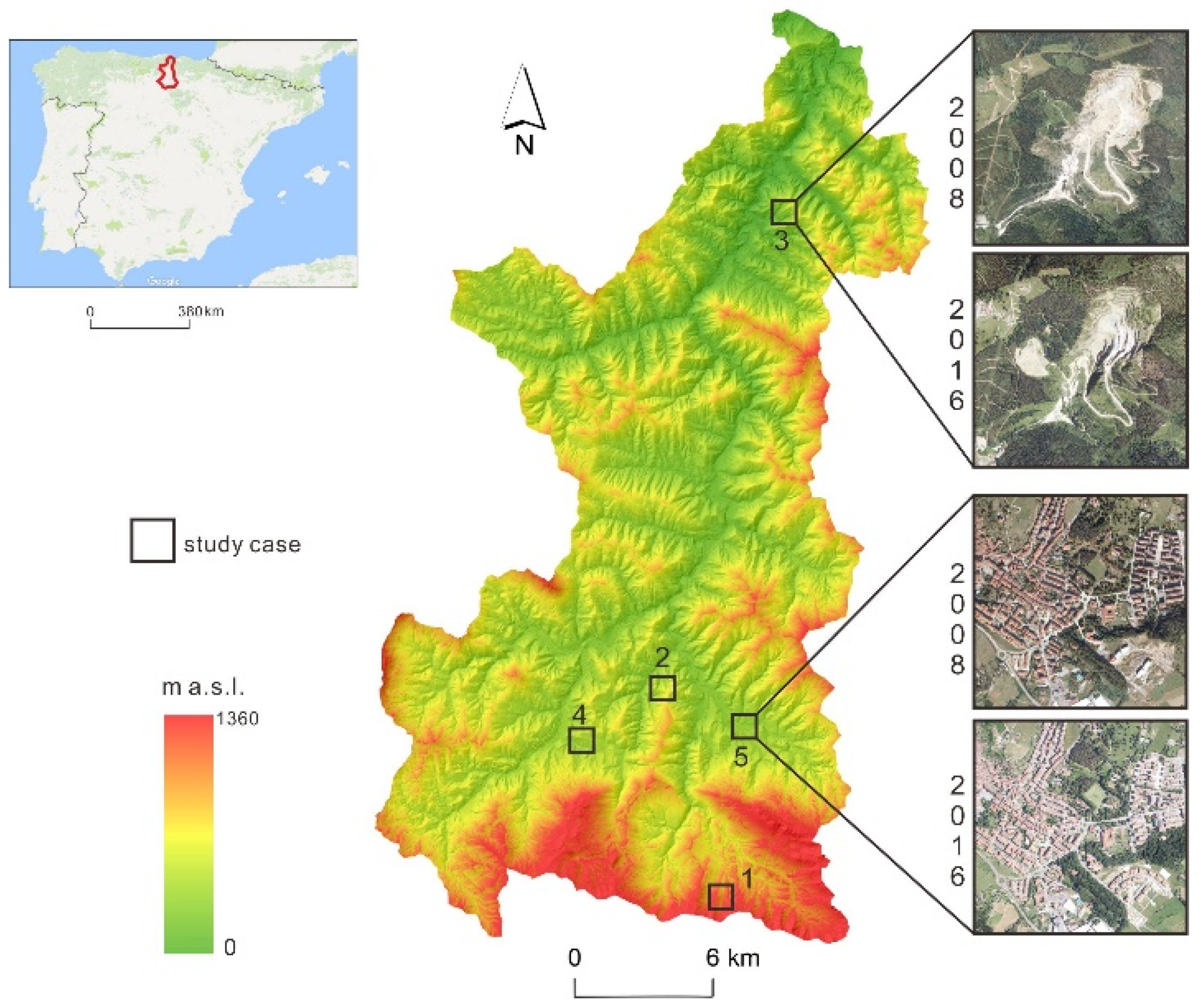
The study was carried out on the Eibar watershed, in Spain. The watershed is part of the Gipuzkoa province (Figure 1), and it covers an area of about 522 km2 with more than 50% forest coverage. The altitude of this catchment ranges from 0 to 1360 m a.s.l. (average of 450 m a.s.l.). Its slope ranges between 0° and 86° (average 23°). Overall, the height gradient follows a North–South direction (higher in the south, lower in the north). The oceanic climate gives this area an intense green color with little thermic oscillation. There are three important cities in this basin: Mondragón, Eibar and Oñati, which are mainly responsible for the development of the anthropogenic surface within this catchment over the years. The cities are accompanied by a dense road network, that covers about 2800 km and has an average density of ~5.4 km/km2.
Geologically, the study area is covered by Flysch formations, which are strips of material of Tertiary well-stratified prevalently sandstones, limestone and shales. Therefore, quarrying is an important economic activity, with more than 10 active quarries. The more natural part of the watershed is included in some natural reserves (the Aizkorri-Aratz, Urkiola and Arno natural parks), mainly distributed in the south and north part. The area presents also two water reservoirs: Urkulu (of about 0.8 km2) and Aixola (of about 0.8 km2) (Figure 1). These reservoirs have been masked during the analysis in order to avoid volumetric changes induced by possible changes in the water level.
Data for the study area have been collected thanks to open access projects of “Gipuzkoa Spatial Data Infrastructure” and the “OpenStreetMap (OSM)” [20,21]. The considered LiDAR dataset (1 m DEMs for the year 2008 and 2016) is free to download from the Gipuzkoa web map viewer, and it has already been successfully applied in the past [10]. The point density of the original LiDAR point cloud was about 2 pts/m2, with a vertical accuracy of 0.1 m on flat horiziontal terrain and a horizontal accuracy of 0.7 m [10]. We also downloaded further information for the same years from the OSM project, which is the largest sources of “Volunteered Geographic Information (VGI)” [22,23]. It is worth pointing out the VGI, which is a new type of information that aims to create free digital world map in Open Source projects. Several researchers have suggested that the OSM project has fairly accurate information [22,23,24].
For a detailed analysis of the anthropogenic features, five small-scale study cases (1×1 km squared) were chosen. These study cases were selected as benchmarks of possible anthropogenic or natural landscapes, and they intentionally included natural reserves, plantations, open-pit mining, agriculture, and urban areas (Figure 1).
3. Method
3.1. Slope Local Length of Auto-Correlation (SLLAC)
Tarolli and Sofia [1] underlined that human activities alter the frequency of occurrence of some specific slope values, even if all slope values are found in the natural and anthropogenic landscapes. Some authors have also pointed out that natural slopes are expected to change rapidly, and neighboring areas can exhibit low correlations; at the same time, anthropogenic slopes are expected to show a reduced variability and demonstrated a high correlation with neighbouring areas [25]. Slope Local Length of Auto-correlation (SLLAC) focuses on local slope similarities and quantifies these similarities based on a 2D cross-correlation between a slope patch and its surrounding areas.
The original SLLAC calculation begins with a slope map derived from the DTM (or DEMs), by computing the slope as a derivative of the quadratic-based polynomial models proposed by Evans et al. [26]. Statistically, the cross-correlation is a standard method for estimating the degree to which two series are correlated. When the correlation is calculated between a series and a lagged version of itself, it is called autocorrelation. One approach to identifying similarities within an image analyzes the cross-correlation of the image with a suitable mask. Where the mask and the pattern to be found are similar, the correlation will be high. Sofia et al. [19] proposed and tested an approach to evaluate similarities of slopes using as mask a moving window (or kernel) of 100 × 100 m, while the pattern to be sought is a template of 10 m × 10 m, having its centre at the center of W.
Firstly, the cross-correlation is calculated between each slope template (T) and its neighbouring areas (W), according to the formula as follows:
where indices (u, v) and (i, j) are the pixel position of the row and column for every T and its W; meanwhile, the and are the mean slope of the T and its W. Clearly the peaks in this cross-correlation “surface” are the positions of the best matches between the template and the mask. Secondly, the cross-correlation map is thresholded at 37% of its maximum value slope [27]. Finally, slope similarities are classified based on the extracted areal autocorrelation that contains the template center and measuring the so-called correlation length, defined as the longest chord passing through the center of the extracted areal autocorrelation (Figure 2). The final SLLAC map is then a value of the autocorrelation length in each pixel. Please refer to [10,19] for a full description of the procedure.
The SLLAC map can be characterized by the Spc (arithmetic mean peak curvature), which represents the arithmetic mean of the principal curvature of the peaks on the surface.
where x and y refer to the cell spacing, n represent the number of peaks, and z is the SLLAC value.
Smaller values of Spc (regular morphology) indicate a possibly more anthropogenic surface, while higher values (high complexity and irregular morphology) of the index represent natural surfaces. Actually, Chen et al. [28] developed a polynomial approach defining a specific relationship between the Spc and the percentage of the anthropogenic surface within the analyzed area, following
where Ant% is the percentage of anthropogenic surface, Spc is obtained from Equation (2), and j1 to j4 are empirically derived coefficients with values of 2.402e + 07, −2.892e + 06, 1.087e + 05, and −1209, respectively.
To better explore the potentialities of SLLAC in diverse environments or conditions, we computed the SLLAC and Spc over the whole basin, and then the average SLLAC () and Spc were computed using a square moving window of 1 km2, thereby providing an analysis of the two parameters in m/km2 and m−1/km2 [10].
3.2. DEM of Difference (DoD)
The DoD approach consists of two DEMs (or DTMs) with the same geodetic control being subtracted (subtracting an earlier one from a later one) [14], while taking into account uncertainty (measurement errors, topographic complexity, geodetic control, interpolation and resolution [14]) () of the DTMs themselves. In this study, we applied a user-defined threshold to distinguish the real geomorphic changes from noise. This is partly due to its simplicity of implementation, as well as because the magnitude of geomorphic change is far greater than the survey errors.
Brasington et al. [17] showed the propagated uncertainty () of the DoD can be calculated using Gaussian error propagation as:
where and are the individual errors in new and old DTMs respectively. By assuming that estimates of are the standard deviation error, the result is a normal distribution with a mean of zero. The absolute values of each grid cell in the DTM of difference (| − |) are then related to to calculate t score by using Equation (5), and a simple t is conducted for each cell to decide whether the change is noise or not.
where can be estimated by a stable area approach [15]. For more details, see [12] and [18].
In this study, we used a probabilistic thresholding method, with a user-defined confidence interval of 95%. Thanks to the open-source software package Geomorphic Change Detection 6 (GCD 6) toolbar (http://gcd6help.joewheaton.org/home), we calculated the geomorphic changes of the whole basin.
3.3. Spatial Autocorrelation
One of the principles of anthropogenic geomorphology is that within regions influenced by a given society, the functions that create anthropogenic features are not homogeneous, but rather differ across space in relation to both social and natural patterns [29]. Patterns of statistical self-similarity or autocorrelation may prove capable of identifying differences between natural geomorphology and anthropogenic ones [19,29,30]. Therefore, to further characterize the different categories of geomorphic changes, we evaluated their spatial autocorrelation. We used the Global Moran’s I [31] index, which measures spatial autocorrelation based on both feature locations and feature values simultaneously. Given a set of features and an associated attribute, it evaluates whether the pattern expressed is clustered, dispersed, or random, and is evaluated as:
where is the spatial weight between feature i and j, and n is equal to the total number of features. The value of I is between −1 and 1. If I is greater than 0, there is positive spatial autocorrelation, and if I is lower than zero, there is negative spatial autocorrelation. The higher the absolute value of I, the greater the positive (or negative) spatial autocorrelation. An I value close to zero represents a random spatial distribution with no spatial autocorrelation.
3.4. The Workflow of the Method
In Chen et al. [28] and Sofia et al. [10,19,32], anthropogenic or artificial landscapes are classified based on the premises that anthropogenic morphologies are expected to be self-similar at a longer distance (higher ) and better-organized (lower Spc) than would be true of a natural morphology. The mentioned literature, however, focused on specific land uses at a time (e.g., terraces vs. natural, different levels of mining activities, and road network and urban area complexity).
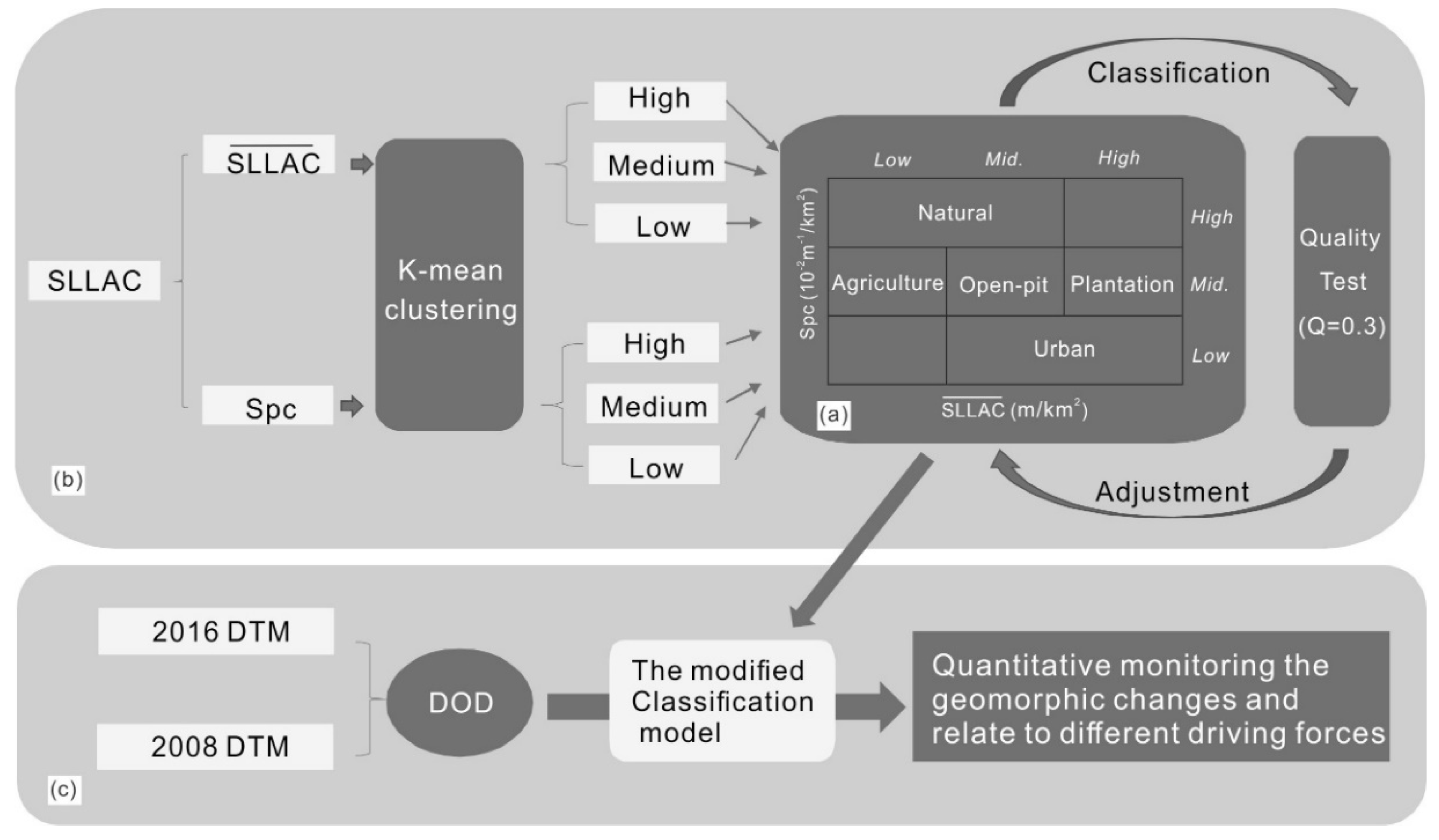
With the aim of developing a more comprehensive method, we proposed an initial model to classify the anthropogenic morphologies in this study area (Figure 3a). The model consists of five hypotheses:
- Natural reserves should be characterized by high disorganization of slope (the presence of vegetation on a LiDAR DTM will still leave a rougher surface the denser the vegetation is, due to the number of pulses that can penetrate the canopy). As a consequence, the topography should be characterized by high Spc and medium to low
- Plantations should be characterized by similar patterns of the slope, but with a higher degree of organization, since plant location is specifically designed through projects and species selections. Consequently, topographies under plantations should be characterized by medium values of Spc and low ;
- Moving towards more ‘artificial’ landscapes, agricultural areas should be characterized by medium Spc values, but high , since the landscape would be mostly flat or ‘flattened’ to allow for machinery access;
- Urban areas are likely to be self-similar at distances shorter than that of agricultural areas, and they would display a much higher degree of organization in the landscape than a natural landscape. As a consequence, they should be characterized by a low Spc and medium to high ;
- Open-pit mining is characterized by long terraces; therefore, the topography for these areas should be characterized by medium Spc and the medium .
We tested these 5 hypotheses in the 5 typical study cases (1 km2 for each area) and verified the classification model in the whole basin at large scale (about 522 km2). According to the capability of the classification model, we identified these geomorphic changes to be due to different driving forces (Figure 3).
The overall workflows proceeded as follow:
(1) The average SLLAC () and Spc were computed, then the map and Spc map were clustered (using a K-means clustering algorithm) to partition each dataset into three categories (low, medium, high). The K-means [33] is one of the most popular and simple clustering algorithms, and it is still one of the most widely used algorithms for clustering, due to its ease of implementation, simplicity, efficiency, and empirical success [34]. For more details, see [35].
(2) We tested the classification model at small and large scales (Figure 3b). It is worth pointing out that these 5 study cases at small scale were already labelled with different landscapes. We were able to analyze the Spc value and average SLLAC value for each study case, and compare the accuracy of the classification model directly. At large scale, the whole basin was classified based on the classification model, and the results needed to be compared to the geographic database of the OSM project, by overlapping the classified surfaces to different landuse. Furthermore, to better test the model, especially for urban areas, the Urban Complexity Index (UCI) (in pts/km2) was computed with point data for the number of buildings and the junctions of road networks, following [32]. This index represents the complexity of the urban system/road network. For our analysis, we argue that the UCI is a good index to extract urban area or other anthropogenic elements (with a suitable threshold), which could be used to test the hypothesis. To assess the quality of the automatic extraction of these landscapes, we used a quality index [36].
where the matching classified areas are defined as true positives (TPs), the un-matching classified areas are considered false positives (FPs), and the landscapes that are not identified by the hypothesis model are designated as false negatives (FNs). The index is arranged from zero to one, with zero representing no overlap between extracted and observed features and one meaning that they were perfectly matched [36]. The average of quality (Q) of the other works regarding geomorphic feature extraction from DTM was about 0.3 [16,32,37,38]. Thus, we set 0.3 as the threshold value of the quality test. If the quality test was greater than this threshold, we believe that the hypothesis model is appropriate, while we adjusted the classification model until it reached the threshold.
(3) We calculated the geomorphic changes of the whole basin using the DoDs based on the multi-temporal DTM (in 2016 and 2008). Meanwhile, we classified the whole basin according to the adjusted model (Figure 3c). By combining the DoDs and the results of the classification, we were able to monitor the geomorphic changes and identify the driving forces are behind the changes.
4. Results
4.1. Test Hypotheses in the 5 Case Studies
Figure 4 shows the images, DTMs, SLLAC and derived parameters map of the small study cases.
The SLLAC map texture is characterized by elongated elements, defined as fibers in [19]. These fibers are mainly located within the mining area, road networks, and terraces (Figure 4k–o). When observing the map (Figure 4p–t) and Spc map (Figure 4u–y) of these study cases, it appears (as expected) that the areas presenting more anthropogenic features (such as mining, road, terraces) will likely have a lower Spc value and higher . This confirms the idea of Sofia et al. [10]: anthropogenic morphologies are expected to be self-similar at a longer distance (higher ) and better-organized (lower Spc) than natural morphologies. This idea is the premise for the classification model based on the LiDAR DTM.
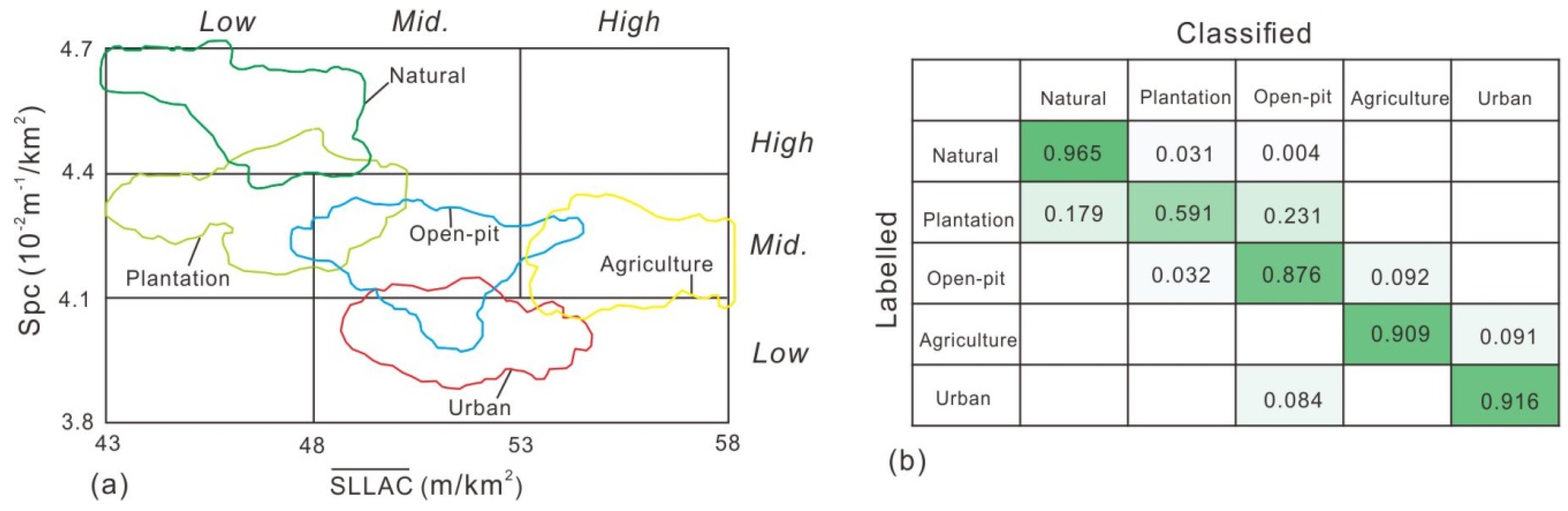
After a first visual assessment, we counted the Spc values compared to the average SLLAC value for each study case (Figure 5a). In this regard, the urban area has the lowest Spc value (3.9 × 10⁻²~4.1 × 10⁻² m−1/km2) and medium to high (48.8~54.5 m/km2). On the contrary, the natural area has the highest Spc value (4.3 × 10⁻²~4.7 × 10⁻² m−1/km2) and low to medium (42.3~49.2 m/km2). Meanwhile, the plantation, open-pit and agriculture land have a medium Spc, but different : the agriculture land has the highest (53.2~58.3 m/km2), followed by the open-pit (47.1~54.4 m/km2) and then the plantation (42.9~50.3 m/km2).
Every small-scale study case, representing the typical anthropogenic feature, was identified and labeled manually from the image. Figure 5b shows the classification accuracy of the initial model for each category. It can be observed that the initial model area obtained the best performance in the natural area (accuracy = 0.965), followed by the urban area (accuracy = 0.916), the agriculture area (accuracy = 0.909), and the open-pit area (accuracy = 0.876). Partly because of the unified planning of the plantation area and partly because it is similar to the natural forest, the plantation area was mis-classified as open-pit (about 23.1%) and natural area (about 17.9%). Therefore, the plantation area had the worst performance (accuracy = 0.591). Overall, the initial model shows a good performance in the small-scale study area.
4.2. Test Hypotheses in the Whole Basin
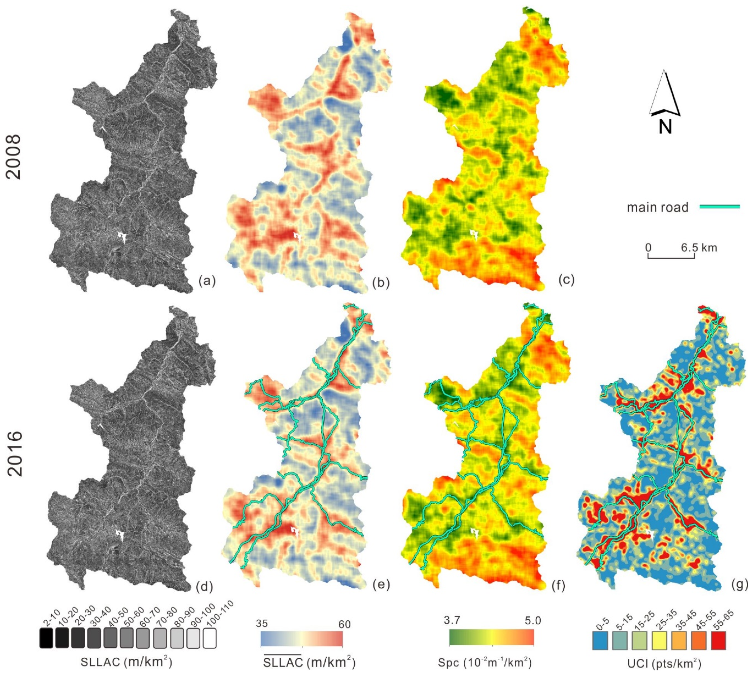
Figure 6 shows the SLLAC and derived parameters map of the whole basin in 2008 and 2016.
When observing the SLLAC maps of the whole basin in 2008 (Figure 6a) and 2016 (Figure 6d), it appears that the anthropogenic structures, especially the main road, create elongated elements. The UCI map confirmed the fact that most of the residential areas are along the main roads in this basin. The areas of the two reservoirs present “NoData” here, due to being masked. As to the maps, both in 2008 and in 2016, there is a strong positive correlation between the value and the UCI, which is representative of the complexity of urban areas. On the contrary, the Spc map shows a strong negative correlation to the UCI map.
After a first visual assessment, we quantified these correlations by calculating Pearson’s coefficient between (also Spc) and Urban complexity index. The result shows that the Pearson’s coefficient was greater than 0.6 for the and UCI, and less than −0.6 for the Spc and UCI. This result is in line with the result provided by Sofia et al. [10,25], where the Pearson’s coefficient had an absolute value greater than 0.6. This strong correlation confirms the fundamental premise of our hypothesis, which is the and Spc can relate geomorphic changes to their different driving forces.
Figure 7 shows the boxplot of the and Spc of the clustering by using the K-mean algorithm in 2008 and in 2016.
By applying the K-mean algorithm, the and Spc was clustered to three categories. For the values of 2008, the “Medium” range refers to 45.623~50.539 m/km2, the “High” represents values greater than 50.539 m/km2 and “Low” means smaller than 45.623 m/km2. As to the Spc of 2008, the “Medium” range refers to 4.225 × 10⁻²~4.424 × 10⁻² m−1/km2, and “High” and “Low” represent values greater/lower than this range, respectively.
For the results of 2016, the “Medium” range refers to 45.742~50.745 m/km2, and the “Medium” Spc represents the range of 4.214 × 10⁻²~4.418 × 10⁻² m−1/km2. Considering the changes of the “Medium” from 2008 to 2016, even though very slight, the increased and the Spc decreased, which is in line with the fact that the basin keep urbanizing during these eight years.
Figure 8 shows the classification results of the 2016 LiDAR DTM based on the initial hypothesis model. For clarity, Figure 8 also displays the buildings (red line) and the boundary of the natural parks (blue line) from the “OpenStreetMap project” in 2016. Most of the buildings are located in the “urban” landscape, where the topography has lower Spc values and the medium to high . At the same time, the natural park well overlaps the area classified as ‘natural’, with high Spc values and low to medium . The classified urban area is mainly located on the valley bottom, while the “natural” area is mostly on the ridges with higher elevation, and this reflects the fact that the urbanization process in a hilly/mountainous context is mostly limited by elevation [39]. The other classified anthropogenic features are mainly located on the hillsides. Overall, “agriculture” areas are closer to the “urban”, which was expected due to the process of evolution of societies [29]. Plantation and natural reservoirs are also clustered together. The “open-pit” areas are instead distributed in a dispersed fashion, which was expected because mining activities are generally localized in space.
Table 1 shows the quality test of the initial hypothesis model compare to the land-use and UCI index from the OSM project in 2016.
When using the UCI index, the areas with higher UCI values (UCI > 55 pts/km2) were identified as urban areas, whereas those with lower UCI value (UCI < 5 pts/km2) were considered natural areas. Our results indicate that the initial model obtained relatively good performance in urban areas, no matter which evaluation criteria were used (Q = 0.37 for Land-use and Q = 0.43 for UCI index). Even in a natural area, the initial model also achieved satisfactory results (Q = 0.31 for Land-use and Q = 0.30 for UCI index), because the average of quality (Q) of the other works about feature extraction from DTM was about 0.3 [16,32,37,38]. These results confirmed the hypothesis that: (a) the landscape of the urban city determines a morphology that is better organized (Low Spc) and self-similar at a longer distance (Medium to High ); (b) the morphology of natural areas is characterized by being less organized (High Spc) and less self-similar (Low to Medium ) (Figure 3a).
However, the three other hypotheses in the initial model turn out to be incorrect. These three other hypotheses mean that areas with medium Spc value while having low probably were probably the “plantation” (Q = 0.10), those medium were probably the “open-pit” (Q = 0.11), and those with high were likely to be “agricultural” areas (Q = 0.05).
Ellis and Ramankutty [40] and Tarolli et al. [29] considered that most anthropogenic biomes are characterized as heterogeneous landscape mosaics, combining a variety of different land use and land covers (e.g., urban areas are embedded within agricultural areas, and trees are interspersed with croplands and housing), which follows the evolution of the underlying society. Therefore, we proposed the “Mosaic area” to combine the areas of “agriculture”, “open-pit”, “plantation” and other land-use, where the direct interactions between humans and ecosystems generally take place [41]. Subsequent to this modification, the quality of the “Mosaic area” reached 0.36~0.38, and the average quality of all three types was greater than the threshold (Q = 0.3) (Table 1).
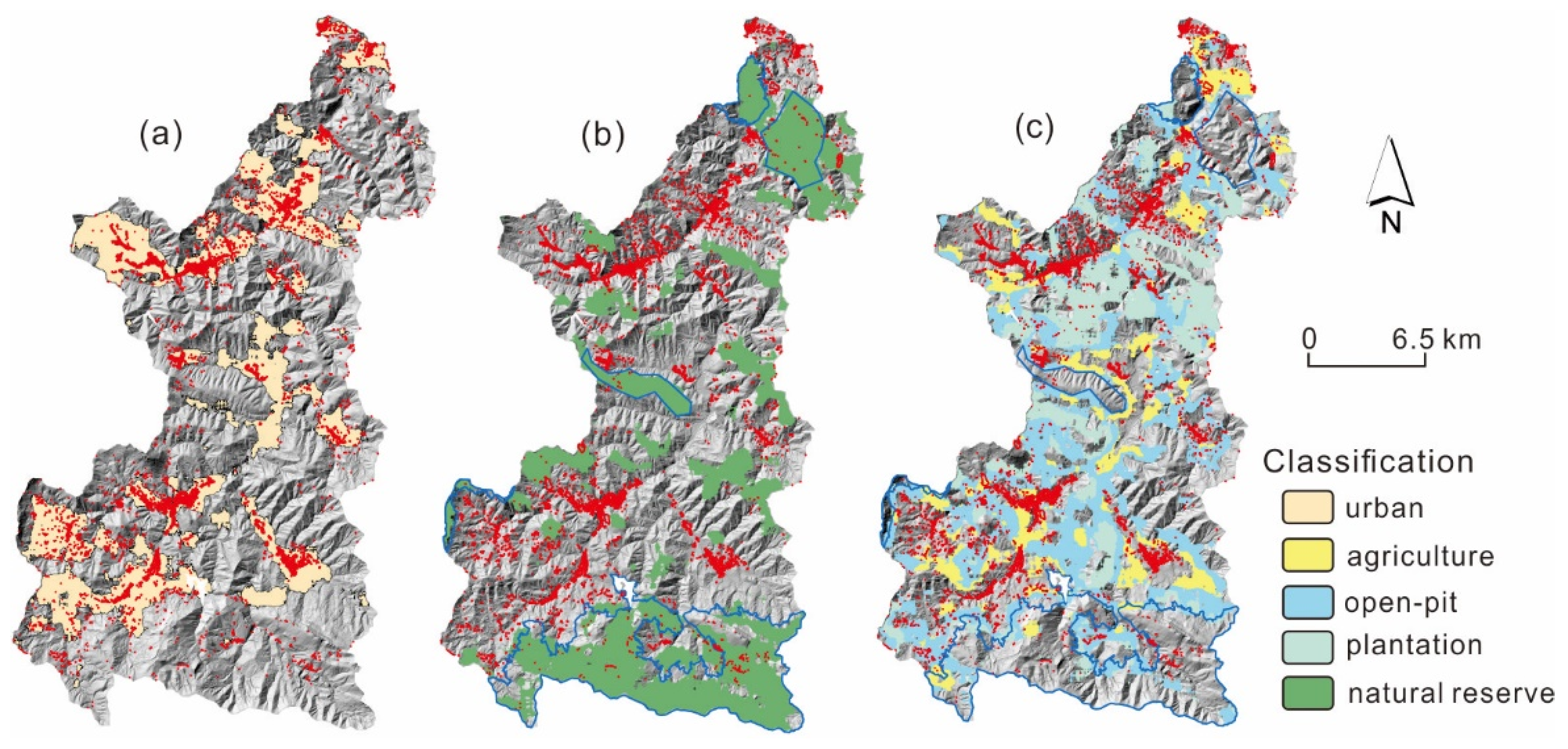
Figure 9 shows the final result of the classification based on the modified model (Figure 9c), which combined the areas where neither “Urban area” nor “Natural area” to the “Mosaic area”. Comparing the classification of these two years (Figure 9a,b), there were few changes occurring in the period 2008–2016.
4.3. Quantitative Detection of the Geomorphic Changes
We applied the polynomial in Equation 3 to define the percentage of the anthropogenic landscape in each sub-area for the two years considered. Table 2 quantifies the areas and proportions of each classification in 2008 and 2016. The “mosaic area” almost remains unchanged and covers more than 50% of the whole basin in this period. The “natural area” makes up 26.26% in 2008; with a decrease of about 1.7 km2, the proportion is reduced to 25.93% in 2016. Meanwhile, the “urban area” increases from 23.66% to 24%. According to the polynomial, proposed by Chen et al. [28], the percentage of the estimated artificial surface of about 25.84% in 2008, and 26.26% in 2016, which is very close to the “urban area” (Table 2). Chen et al. [28] proposed this polynomial for mining landscapes at the local scale (about 3 km2); the artificial surface refers to the terraced area. However, in this research, at a basin scale (about 522 km2), the estimated artificial surface most likely refers to the “urban area”. This result confirms the effectiveness of this polynomial and expands the scope of application (from small scale to large scale, and from single to comprehensive environmental context).
Despite the fact that the initial hypothesis model is proved only partially correct, the modified model (Figure 9c) will help to provide more information about anthropogenic geomorphology. However, considering the accuracy and the changes of the classification in this period, there is no necessity to discuss the areas in which the category is changed. For example, the area was labelled “natural” in 2008, and was then classified as “mosaic” in 2016. Because the changes are small (smaller than 1%) and the method is not sensitive enough, we use the classification of 2016 to understand the geomorphic changes in the next section.
Figure 10 shows the DoD map in the period of 2008 to 2016, and segregated by the classification of the modified model in 2016.
In these eight years, geomorphic changes (high DoD) mainly happened in “mosaic” and “urban” areas, while lower DoD values were located in the “natural” area. With regard to elevation changes, “mosaic” mainly ranged from −18 m to 15 m, while “urban” ranged from −12 m to 13 m, and “natural” ranged from -8 m to 5 m. Considering the shape and elevation changes of the DoD, especially in the southern part, the driving forces mean that the changes in “urban area” were probably due to the construction of an expressway in the south of this basin (Figure 10c), due to being line-shaped. Meanwhile, the DoD in the natural landscape is spot-shaped and sporadically distributed (Figure 10a); therefore, the forces may be some geological hazard (such as landslide, collapse or debris flow).
The volumetric elevation change distributions (ECDs) are histograms showing the total volume experiencing a given magnitude of elevation change in each bin [12]. Figure 10d–f represents the volumetric ECDs of “natural”, “mosaic” and “urban”, respectively. It appears that “mosaic” and “urban” made up most of the volumetric change. The “natural” of volumetric ECDs shows a strong asymmetry, compared to the other two, the erosion volume is three times that of the deposition.
Table 3 reports the areal and volumetric DoD from 2008 to 2016.
Overall, the “urban” area had the most intensive geomorphic changes (erosion volume = 7,998,829 m3 and deposition volume = 9,945,932 m3), followed by the “mosaic” area (erosion volume = 7,141,480 m3 and deposition volume = 7,967,817 m3). In the two areas, the total net volume had positive values (1,947,103 and 826,337 m3); on the contrary, the “natural” area had a negative value (-1,981,214 m3). These results show that the deposition process is greater than the erosion process in “urban” and “mosaic” areas, and quite the reverse in “natural” areas.
With regard to the changing area, the “urban” area exhibited the greatest change (0.39% for erosion and 0.50% for deposition), followed by the “mosaic” are (0.31% for erosion and 0.42% for deposition), and the weakest was the “natural” are (0.08% for erosion and 0.09% for deposition). As to the volume errors, the “urban” are had the biggest error (±456,635 m3), followed by the “mosaic” area (±377,882 m3), and the lowest was the “natural” area (±90,650 m3) (Table 3).
Another aspect to consider is the erosion rate. We already know the extent of the different types of areas (Table 2), and Table 3 shows the erosion volume in the 8-year timeframe (2008–2016). Therefore, we can evaluate the erosion rate in terms of mm year−1. The “natural” area suffered erosion of about 2.808 mm year−1, the “mosaic” of about 3.488 mm year−1, the “urban” of about 8.153 mm year−1, and the whole basin of about 4.339 mm year−1. The “urban” area had the most intensive erosion rate.
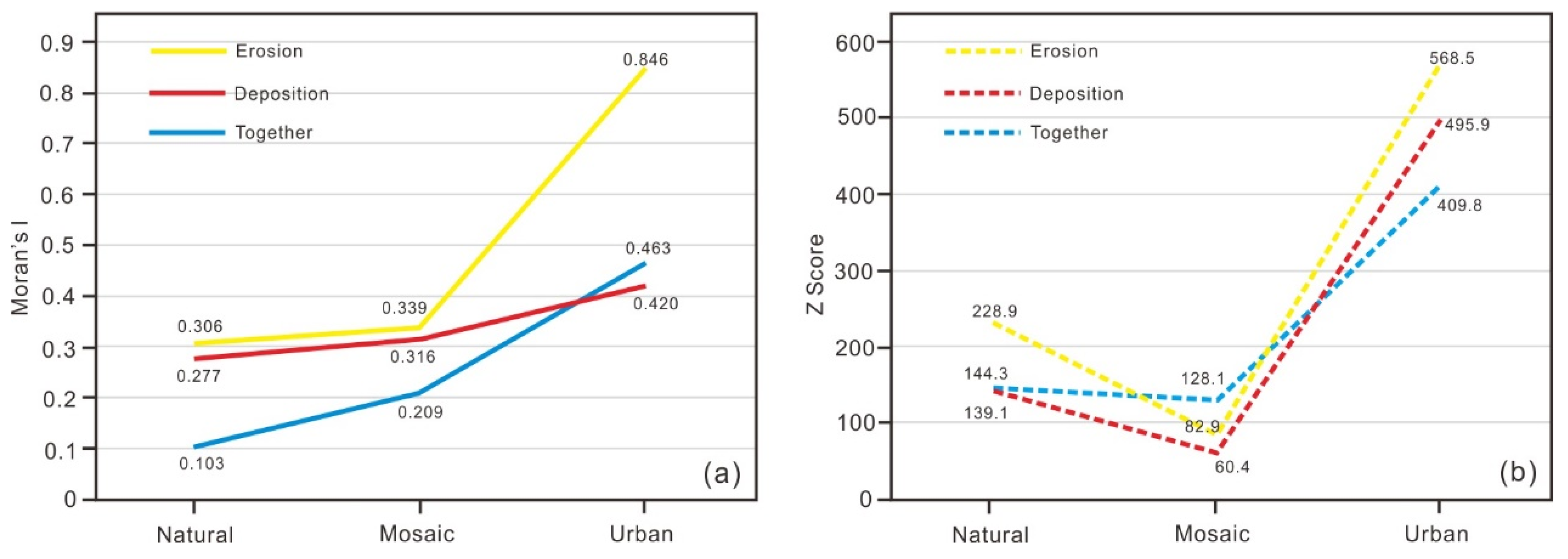
Figure 11 shows the results from the spatial autocorrelation analysis of the geomorphic changes in different categories.
The geomorphic changes represent the volumetric changes, which include three types, including erosion, deposition and total net (denoted as together). According to Figure 11a, all Moran’s I values of different categories were larger than 0, which means a positive spatial autocorrelation. Also, the Z-scores in all different categories were larger than 1.96 (Figure 11b), which generally implies significant spatial autocorrelation at the 0.05 level [42]. Both the Moran’s I value and the Z-score further confirm that the geomorphic changes exhibited a clustered distribution in all categories.
However, the spatial autocorrelation degree varies among the different categories (Figure 11a). On the one hand, in the natural and mosaic areas, the volumetric erosion changes have the most visible manifestation of the spatial autocorrelation characteristic (Moran’s I = 0.306 for natural and 0.339 for the mosaic), followed by deposition (Moran’s I = 0.277 for natural and 0.316 for the mosaic) and then the total net (Moran’s I = 0.103 for natural and 0.209 for the mosaic). However, the overall net volumetric changes show a stronger positive spatial autocorrelation than deposition (Moran’s I = 0.463 for the total net and 0.420 for deposition) in the urban area. On the other hand, no matter which kinds of geomorphic changes are considered, the urban area has the highest Moran’s I value, followed by the mosaic and then the natural area.
5. Discussion
The Anthropocene has been widely and deeply discussed by geomorphologists, and the most important issue is what exact roles humans have played in shaping the geomorphology of landscapes over the past few millennia [1,9]. There is no doubt that human activities are now transforming the geomorphology of landscapes at increasing rates and scales across the globe. Hooke [43] argued that humans are “geomorphic agents”, comparing them to land-shaping forces of nature, such as rivers, glaciers, rain and wind. However, some authors believe anthropogenic forces to be often difficult to separate from natural forces [44]. The proposed analysis shows that geomorphic changes in landscapes with a greater human disturbance (mosaic and urban) tend to be more spatially correlated than natural processes (Figure 11). This result of the spatial autocorrelation analysis might help to identify the forces of the geomorphic process.
The urban area in this study case, furthermore, shows a greater correlation in erosion (i.e., materials removed from the landscape) rather than in deposition (i.e., materials re-deposited). One must remember that, like some other surficial geomorphic processes (e.g., dune formation), anthropogenic geomorphic changes are often not unidirectional, with materials moved back and forth, and upward and downward, and movements driven by many different pathways and processes. The removed materials and the deposited ones might not necessarily correspond, and differences of constituent materials also cause significant differences in the individual scale and morphological features of anthropogenic changes. The results show that human-induced changes tend to a more clustered distribution. This finding is in line with other works dealing with urban structures [45,46,47,48], but it adds multidimensional perspective in terms of volume of changes, not just in terms of spatial structures.
Wilkinson [49] suggested that human activities shift ten times as much material on the Earth’s surface as all natural geological processes put together, based on the estimate of the natural soil and sediment movement on the rate at which sedimentary rocks have been formed over the past half a billion years. The measurement capabilities described in this work, as a result of advances in sensor systems, computational technology, and large-scale data sharing (the work is based on free LiDAR), make the prospect of quantifying processes of anthropogenic geomorphic change globally over the long term a real possibility [6].
We provide the measurement of erosion rate in terms of mm y−1, and this allows for a direct comparison with the other works. For example, Tarolli and Sofia [1] converted published values into mm y−1, and the results showed that the global estimated erosion rate was ~0.4 mm y−1, with that of industrialized countries (such as Britain) reaching ~2 mm y−1. At a watershed scale, the erosion rate ranged from 0.1 mm y−1 to 3 mm y−1, and the erosion rate can reach >10 mm y−1 at a hillslope scale. Obviously, local erosion rates are differently influenced by the scales, slopes, vegetation, rocks and soils.
The results from the methodology we proposed showed that the urban area had the highest erosion rate, followed by the mosaic area and then the natural area. From this point of view, anthropogenic forces are expected to have a greater erosion rate than natural forces. Although we are aware that these results were obtained at watershed scale in a relatively short period, the methodology described in this contribution advances the knowledge in that it offers a convenient tool to assess the erosion rates of different driving forces rapidly and efficiently. This tool makes it possible not only to monitor geomorphic changes and identify the driving forces of such changes, but also to understand the main shapers of Earth’s surface process are, between natural and anthropogenic forces.
With the popularization of LiDAR technology and data accumulation in different environmental contexts at different scales, the proposed framework with new algorithms will be developed, and long-term dynamics mechanisms of Earth’s surface process will be revealed. Furthermore, by combining with the concept of “sociocultural fingerprints”, proposed by Tarolli et al. [29], the proposed methodology will support the observation, identification and interpretation of natural and anthropogenic forces.
6. Conclusions
Human activities are now transforming the geomorphology of landscapes at increasing rates and scales across the globe. There is more and more geomorphological evidence to verify that human societies have become the dominant factors in many contexts at different scales. Moreover, the geomorphic impacts of human activities are likely to be preserved for a long time and damage natural ecosystems. Understanding the mechanisms and consequences of these transformations represents a challenge for better supporting sustainable environmental planning. In this research, based on multitemporal LiDAR topography, we present a useful framework for quantitively detecting anthropogenic geomorphic changes and relating such changes to different driving forces. This methodology combines the effectiveness of SLLAC and derived parameters at reflecting anthropogenic pressures and the advantages of DoD in quantitively detecting geomorphic changes. It also offers a convenient tool for assessing the erosion rates of different driving forces rapidly and efficiently.
Indeed, this ensemble method provides a preliminary, objective and fast analysis of geomorphic changes, while more detailed assessments require the use of more long-term datasets and their application in different environmental contexts at different scales. In the future, we will combine the proposed methodology with the concept of “sociocultural fingerprints”, i.e., based on the societal structure and functioning of the anthropogenic features. The method may help to observe, identify and interpret geo-environmental processes and their possible interactions with humans, providing a better understanding of these mechanisms in order to implement sustainable environmental planning, mitigating the consequences of anthropogenic alteration.
Author Contributions
All authors made substantial contributions to this study. J.X., P.T. and G.S. jointly designed the study, J.X., S.L. and K.X. wrote the manuscript. P.T. supervised the whole work.
Funding
This research was funded by the National Key Research and Development Program of China (No. 2017YFC0601501 and No. 2017YFC0601502), the China National Mineral Resources Assessment Initiative (No. 1212010733806 and 1212011120140). This research was also supported by the University of Padova grant 60A08-5455/15 “the analysis of the topographic signature of anthropogenic processes.”
Acknowledgments
The authors would like to acknowledge the open-source software “KNIME Analytics Platform” and some free download resources, such as LiDAR DTMs from the Diputacion Foral de Gipuzkoa, geographic database from the “OpenStreetMap” project. The authors thank also the anonymous reviewers who helped in improving the work with useful indications.
Conflicts of Interest
The authors declare no conflict of interest.
References
- Tarolli, P.; Sofia, G. Human topographic signatures and derived geomorphic processes across landscapes. Geomorphology 2016, 255, 140–161. [Google Scholar] [CrossRef] [Green Version]
- Wohl, E. Wilderness is dead: Whither critical zone studies and geomorphology in the Anthropocene? Anthropocene 2013, 2, 4–15. [Google Scholar] [CrossRef]
- Tarolli, P. Humans and the Earth’s surface. Earth Surf. Process. Landf. 2016, 41, 2301–2304. [Google Scholar] [CrossRef]
- Hilborn, R. Moving to sustainability by learning from successful fisheries. Ambio 2007, 36, 296–303. [Google Scholar] [CrossRef]
- García-Ruiz, J.M.; Beguería, S.; Nadal-Romero, E.; González-Hidalgo, J.C.; Lana-Renault, N.; Sanjuán, Y. A meta-analysis of soil erosion rates across the world. Geomorphology 2015, 239, 160–173. [Google Scholar] [CrossRef] [Green Version]
- Tarolli, P.; Sofia, G.; Wenfang, C. The Geomorphology of the Human Age. Encycl. Anthr. 2018, 1, 35–43. [Google Scholar]
- Jordan, H.; Hamilton, K.; Lawley, R.; Price, S.J. Anthropogenic contribution to the geological and geomorphological record: A case study from Great Yarmouth, Norfolk, UK. Geomorphology 2016, 253, 534–546. [Google Scholar] [CrossRef]
- Passalacqua, P.; Belmont, P.; Staley, D.M.; Simley, J.D.; Arrowsmith, J.R.; Bode, C.A.; Crosby, C.; DeLong, S.B.; Glenn, N.F.; Kelly, S.A.; et al. Analyzing high resolution topography for advancing the understanding of mass and energy transfer through landscapes: A review. Earth Sci. Rev. 2015, 148, 174–193. [Google Scholar] [CrossRef] [Green Version]
- Tarolli, P. High-resolution topography for understanding Earth surface processes: Opportunities and challenges. Geomorphology 2014, 216, 295–312. [Google Scholar] [CrossRef]
- Sofia, G.; Marinello, F.; Tarolli, P. Metrics for quantifying anthropogenic impacts on geomorphology: Road networks. Earth Surf. Process. Landf. 2016, 41, 240–255. [Google Scholar] [CrossRef]
- Williams, R.D. DEMs of Difference. Geomorphol. Tech. 2012, 2, 1–17. [Google Scholar]
- Wheaton, J.M.; Brasington, J.; Darby, S.E.; Sear, D.A. Accounting for uncertainty in DEMs from repeat topographic surveys: Improved sediment budgets. Earth Surf. Process. Landf. 2010, 35, 136–156. [Google Scholar] [CrossRef]
- Lane, S.N.; Richards, K.S.; Chandler, J.H. Developments in monitoring and modelling small-scale river bed topography. Earth Surf. Process. Landf. 1994, 19, 349–368. [Google Scholar] [CrossRef]
- Brasington, J.; Rumsby, B.T.; McVey, R.A. Monitoring and modelling morphological change in a braided gravel-bed river using high resolution GPS-based survey. Earth Surf. Process. Landf. 2000, 25, 973–990. [Google Scholar] [CrossRef]
- Westaway, R.M.; Lane, S.N.; Hicks, D.M. The development of an automated correction procedure for digital photogrammetry for the study of wide, shallow, gravel-bed rivers. Earth Surf. Process. Landf. 2000, 25, 209–226. [Google Scholar] [CrossRef]
- Prosdocimi, M.; Calligaro, S.; Sofia, G.; Dalla Fontana, G.; Tarolli, P. Bank erosion in agricultural drainage networks: New challenges from structure-from-motion photogrammetry for post-event analysis. Earth Surf. Process. Landf. 2015, 40, 1891–1906. [Google Scholar] [CrossRef]
- Brasington, J.; Langham, J.; Rumsby, B. Methodological sensitivity of morphometric estimates of coarse fluvial sediment transport. Geomorphology 2003, 53, 299–316. [Google Scholar] [CrossRef]
- Vericat, D.; Wheaton, J.M.; Brasington, J. Revisiting the morphological appoach: Opportunities and challenges with repeat high resolution topography. Gbr8 2015, 1–45. [Google Scholar]
- Sofia, G.; Marinello, F.; Tarolli, P. A new landscape metric for the identification of terraced sites: The Slope Local Length of Auto-Correlation (SLLAC). ISPRS J. Photogramm. Remote Sens. 2014, 96, 123–133. [Google Scholar] [CrossRef]
- Corcoran, P.; Mooney, P.; Bertolotto, M. Analysing the growth of OpenStreetMap networks. Spat. Stat. 2013, 3, 21–32. [Google Scholar] [CrossRef] [Green Version]
- Neis, P.; Zielstra, D. Recent Developments and Future Trends in Volunteered Geographic Information Research: The Case of OpenStreetMap. Future Internet 2014, 6, 76–106. [Google Scholar] [CrossRef] [Green Version]
- Neis, P.; Zipf, A. Analyzing the contributor activity of a volunteered geographic information project—The case of OpenStreetMap. ISPRS Int. J. Geo-Inf. 2012, 1, 146–165. [Google Scholar] [CrossRef]
- Haklay, M. How good is volunteered geographical information? A comparative study of OpenStreetMap and Ordnance Survey datasets. Environ. Plan. B Plan. Des. 2010, 37, 682–703. [Google Scholar] [CrossRef]
- Lin, Y. A qualitative enquiry into OpenStreetMap making. New Rev. Hypermedia Multimed. 2011, 17, 53–71. [Google Scholar] [CrossRef]
- Passalacqua, P.; Belmont, P.; Foufoula-Georgiou, E. Automatic geomorphic feature extraction from lidar in flat and engineered landscapes. Water Resour. Res. 2012, 48, 1–18. [Google Scholar] [CrossRef]
- Evans, I.S. An Integrated System of Terrain Analysis and Slope Mapping: Final Report on Grant DA-ERO-591-73-G0040; Durham University: Durham, UK, 1979. [Google Scholar]
- International Organization of Standardization (ISO). 25178-2:Geometrical Product Specifications (GPS)-Surface Texture: Areal-Part 2: Terms, Definitions and Surface Texture Parameters; ISO: Geneva, Switzerland, 2013. [Google Scholar]
- Chen, J.; Li, K.; Chang, K.J.; Sofia, G.; Tarolli, P. Open-pit mining geomorphic feature characterisation. Int. J. Appl. Earth Obs. Geoinf. 2015, 42, 76–86. [Google Scholar] [CrossRef]
- Tarolli, P.; Cao, W.; Sofia, G.; Evans, D.; Ellis, E.C. From features to fingerprints: A general diagnostic framework for anthropogenic geomorphology. Prog. Phys. Geogr. Earth Environ. 2019, 43, 95–128. [Google Scholar] [CrossRef] [Green Version]
- Sofia, G.; Masin, R.; Tarolli, P. Prospects for crowdsourced information on the geomorphic ‘engineering’ by the invasive Coypu (Myocastor coypus). Earth Surf. Process. Landf. 2017. [Google Scholar] [CrossRef]
- Moran, P.A.P. The interpretation of statistical maps. J. R. Stat. Soc. Ser. B 1948, 10, 243–251. [Google Scholar] [CrossRef]
- Sofia, G.; Tarolli, P. Automatic characterization of road networks under forest cover: Advances in the analysis of roads and geomorphic process interaction. Rend. Online Soc. Geol. Ital. 2016, 39, 23–26. [Google Scholar] [CrossRef]
- Steinhaus, H. Sur la division des corp materiels en parties. Bull. Acad. Pol. Sci 1956, 1, 801. [Google Scholar]
- Jain, A.K. Data clustering: 50 years beyond K-means. Pattern Recognit. Lett. 2010, 31, 651–666. [Google Scholar] [CrossRef]
- Arthur, D.; Vassilvitskii, S. K-Means++: The Advantages of Careful Seeding. Proc. Eighteenth Annu. ACM-SIAM Symp. Discret. Algorithms 2007, 8, 1025–1027. [Google Scholar] [CrossRef]
- Heipke, C.; Mayer, H.; Wiedemann, C.; Jamet, O. Automated reconstruction of topographic objects from aerial images using vectorized map information. Int. Arch. Photogramm. Remote Sens. 1997, 23, 47–56. [Google Scholar]
- Tarolli, P.; Sofia, G.; Dalla Fontana, G. Geomorphic features extraction from high-resolution topography: Landslide crowns and bank erosion. Nat. Hazards 2012, 61, 65–83. [Google Scholar] [CrossRef]
- Xiang, J.; Chen, J.; Sofia, G.; Tian, Y.; Tarolli, P. Open-pit mine geomorphic changes analysis using multi-temporal UAV survey. Environ. Earth Sci. 2018. [Google Scholar] [CrossRef]
- Forman, R.; Sperling, D.; Bissonette, J.; Clevenger, A.; Cutshall, C.; Dale, V.; Fahrig, L.; France, R.; Goldman, C.; Heanue, K.; et al. Road ecology: Science and solutions. Rev. Lit. Arts Am. 2003. [Google Scholar] [CrossRef]
- Ellis, E.C.; Ramankutty, N. Putting people in the map: Anthropogenic biomes of the world. Front. Ecol. Environ. 2008, 6, 439–447. [Google Scholar] [CrossRef]
- Daily, G.C.; Söderqvist, T.; Aniyar, S.; Arrow, K.; Dasgupta, P.; Ehrlich, P.R.; Folke, C.; Jansson, A.; Jansson, B.-O.; Kautsky, N.; et al. The Value of Nature and the Nature of Value. Science 2000, 289, 395–396. [Google Scholar] [CrossRef] [PubMed] [Green Version]
- Getis, A.; Ord, J.K. The analysis of spatial association by use of distance statistics. Geogr. Anal. 1992, 24, 189–206. [Google Scholar] [CrossRef]
- Hooke, R.L. On the history of humans as geomorphic agents. Geology 2000, 28, 843–846. [Google Scholar] [CrossRef]
- Fuller, I.C.; Macklin, M.G.; Richardson, J.M. The Geography of the Anthropocene in N ew Z ealand: Differential River Catchment Response to Human Impact. Geogr. Res. 2015, 53, 255–269. [Google Scholar] [CrossRef]
- Thomas, I.; Frankhauser, P.; Biernacki, C. The morphology of built-up landscapes in Wallonia (Belgium): A classification using fractal indices. Landsc. Urban Plan. 2008, 84, 99–115. [Google Scholar] [CrossRef]
- Beck, J.; Sieber, A. Is the Spatial Distribution of Mankind’s Most Basic Economic Traits Determined by Climate and Soil Alone? PLoS ONE 2010, 5, e10416. [Google Scholar] [CrossRef]
- Nolè, G.; Danese, M.; Murgante, B.; Lasaponara, R.; Lanorte, A. Using Spatial Autocorrelation Techniques and Multi-Temporal Satellite Data for Analyzing Urban Sprawl; Springer: Berlin/Heidelberg, Germany, 2012; pp. 512–527. [Google Scholar]
- Liu, J.; Chen, Y. Spatial autocorrelation and localization of urban development. Chin. Geogr. Sci. 2007, 17, 34–39. [Google Scholar] [CrossRef]
- Wilkinson, B.H. Humans as geologic agents: A deep-time perspective. Geology 2005, 33, 161–164. [Google Scholar] [CrossRef]
Figure 1.
Location and topographic map of the Eibar watershed. Typical study case in small scale: (1) natural reserve, (2) plantation, (3) open-pit, (4) agriculture, (5) urban.
Figure 1.
Location and topographic map of the Eibar watershed. Typical study case in small scale: (1) natural reserve, (2) plantation, (3) open-pit, (4) agriculture, (5) urban.

Figure 2.
The calculation of SLLAC for a single moving window W: (a) the slope template (T) and its neighbouring areas (W), (b) the cross-correlation map between T and W, (c) the thresholded map shows that the length of the correlation.
Figure 2.
The calculation of SLLAC for a single moving window W: (a) the slope template (T) and its neighbouring areas (W), (b) the cross-correlation map between T and W, (c) the thresholded map shows that the length of the correlation.
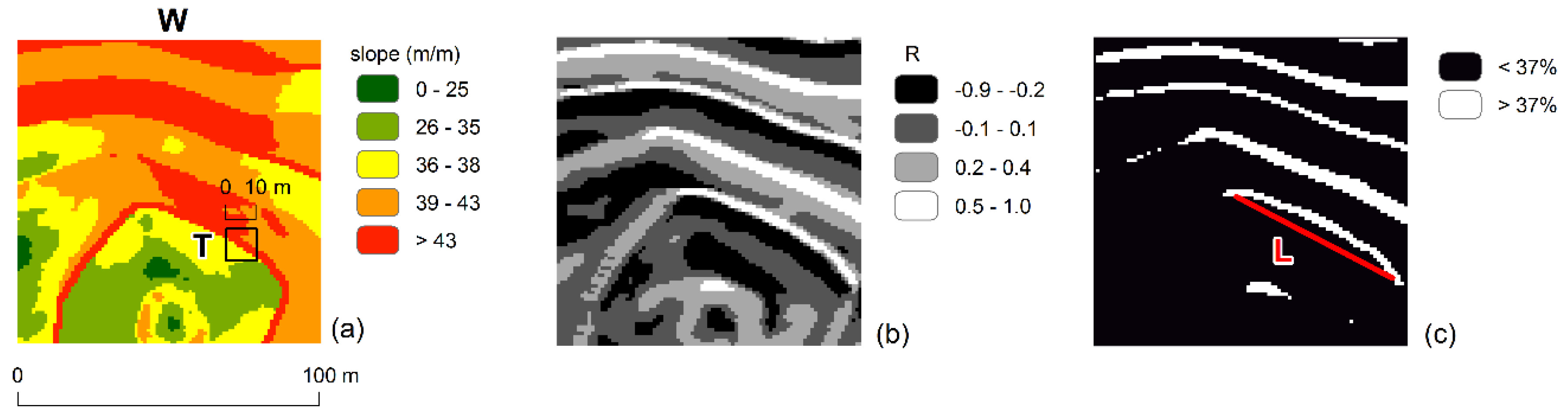
Figure 3.
Workflow of the procedure for the quantitative analysis of the geomorphic changes: (a) the hypothesis model, (b) test and adjust the hypothesis model, (c) quantitative monitoring of the whole basin.
Figure 3.
Workflow of the procedure for the quantitative analysis of the geomorphic changes: (a) the hypothesis model, (b) test and adjust the hypothesis model, (c) quantitative monitoring of the whole basin.

Figure 4.
Analysis of typical study case in small scale: (a) natural reserve, (b) plantation, (c) open-pit, (d) agriculture, (e) urban. (f–j) display the LiDAR DTM for each area. (k–o) represent the original SLLAC and (p–t) represent the derived average SLLAC (), respectively. (u–y) display the derived Spc for each area.

Figure 5.
The statistics of Spc value compare to average SLLAC value for each study case (a), and the accuracy of the classification model for each study case (b).
Figure 5.
The statistics of Spc value compare to average SLLAC value for each study case (a), and the accuracy of the classification model for each study case (b).

Figure 6.
The SLLAC and derived parameters map of the whole basin in 2008 and 2016, and (g) the UCI map based on the geographic database in 2016. SLLAC map: (a) in 2008 and (d) in 2016; map: (b) in 2008 and (e) in 2016; derived Spc map: (c) in 2008 and (f) in 2016.
Figure 6.
The SLLAC and derived parameters map of the whole basin in 2008 and 2016, and (g) the UCI map based on the geographic database in 2016. SLLAC map: (a) in 2008 and (d) in 2016; map: (b) in 2008 and (e) in 2016; derived Spc map: (c) in 2008 and (f) in 2016.

Figure 7.
Boxplot of the (a) and (b) Spc of the clustering by using the K-mean algorithm in 2008 and in 2016.
Figure 7.
Boxplot of the (a) and (b) Spc of the clustering by using the K-mean algorithm in 2008 and in 2016.
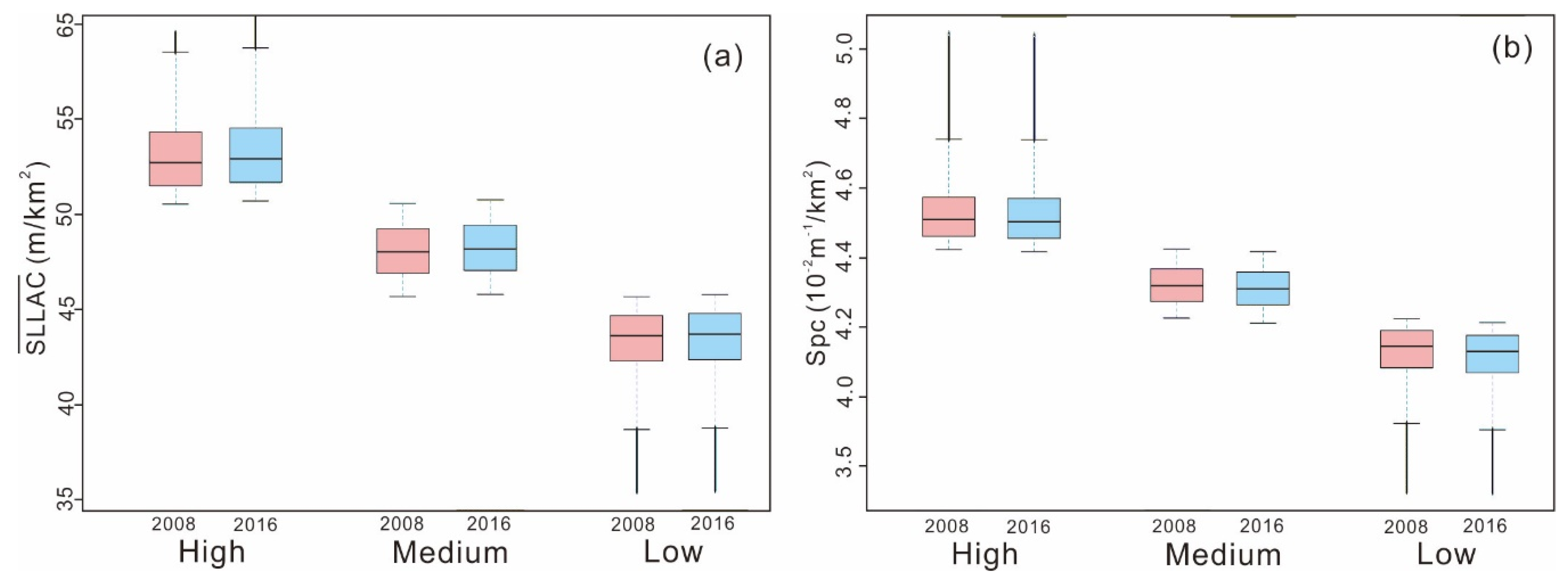
Figure 8.
The classification result of the 2016 LiDAR DTM based on the initial hypothesis model. (a) Extraction of “urban” compared to the buildings (red line); (b) extraction of “natural reserve” compared to the boundary of the natural park (blue line); (c) classification of “agriculture”, “open-pit” and “plantation”.

Figure 9.
The final result of the classificaiton based on the (c) modified model in (a) 2008 and (b) in 2016. In the modified model, the green, orange, and blue lines represent the natural, urban and mosaic areas, respectively.
Figure 9.
The final result of the classificaiton based on the (c) modified model in (a) 2008 and (b) in 2016. In the modified model, the green, orange, and blue lines represent the natural, urban and mosaic areas, respectively.
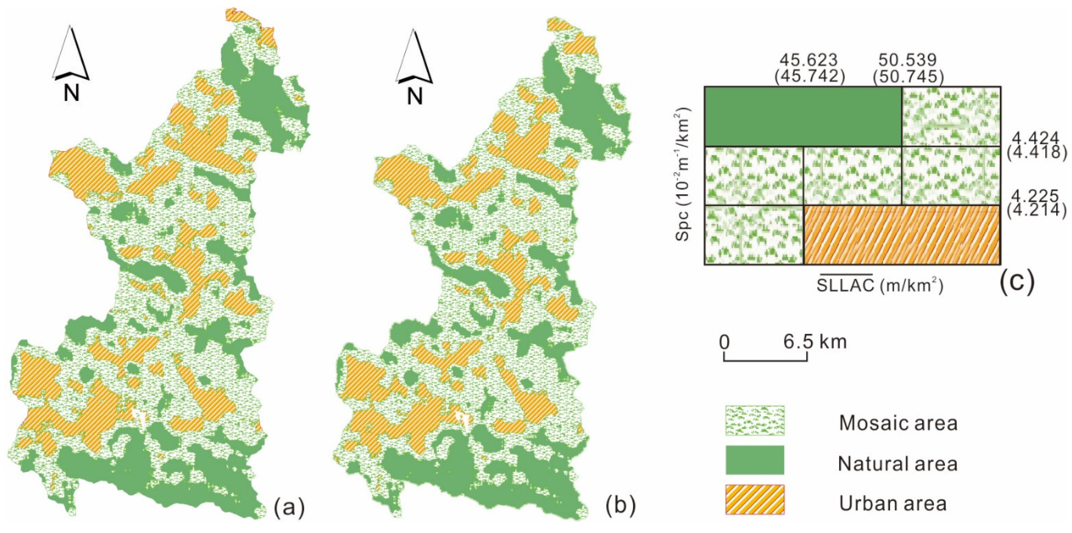
Figure 10.
DTM of difference (DoD) in the period of 2008 to 2016, and segregated by the classification of the final model in 2016. DoD map and volumetric ECDs: (a) and (d) for the “Natural area”, (b) and (e) for the “Mosaic area”, (c) and (f) for the “Urban area”. The red and blue bars represent erosion and deposition, and grey shows the whole basin.
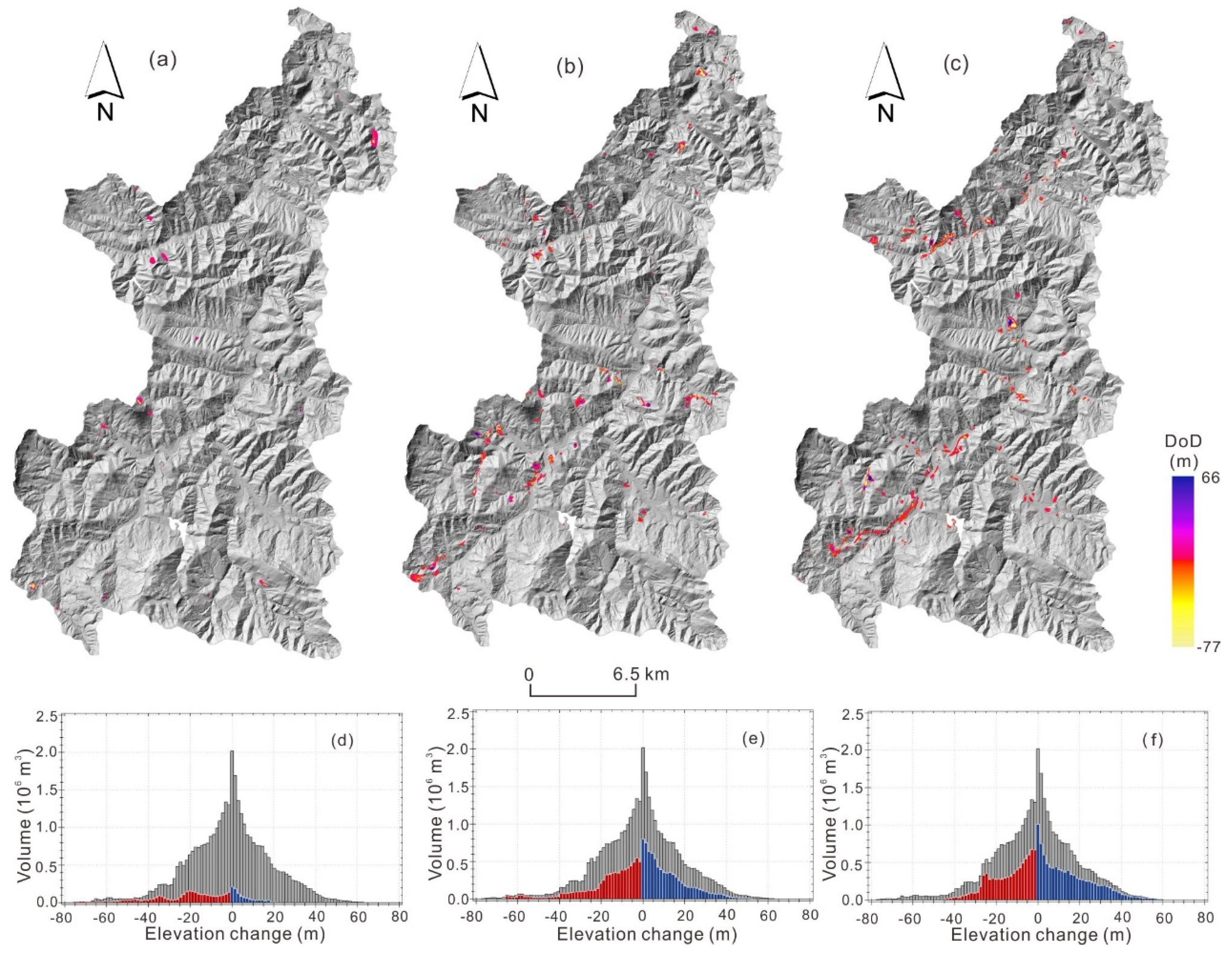
Figure 11.
Spatial autocorrelation of the geomorphic changes in different categories: (a) Moran’s I and (b) Z-score.
Figure 11.
Spatial autocorrelation of the geomorphic changes in different categories: (a) Moran’s I and (b) Z-score.


Table 1.
The quality test of the initial hypothesis model compared to land-use and UCI index from the OSM project in 2016.
Table 1.
The quality test of the initial hypothesis model compared to land-use and UCI index from the OSM project in 2016.
| Classification | Compared to Land-Use | Compared to UCI | ||
|---|---|---|---|---|
| Category | Quality | Range (pts/km2) | Quality | |
| Urban | residential | 0.37 | > 55 | 0.43 |
| Natural | natural park | 0.31 | < 5 | 0.30 |
| Agriculture | farmland | 0.11 | ||
| Open-pit | quarry | 0.05 | ||
| Plantation | woodland | 0.10 | ||
| Mosaic | farmland + quarry + woodland | 0.38 | [5, 50] | 0.36 |
Table 2.
The area and proportions of the classification based on the modified model in 2008 and 2016, and the estimated artificial surface according to the polynomial proposed by Chen et al. [28].
Table 2.
The area and proportions of the classification based on the modified model in 2008 and 2016, and the estimated artificial surface according to the polynomial proposed by Chen et al. [28].
| Classification | 2008 | 2016 | ||
|---|---|---|---|---|
| Area (km2) | Percentage (%) | Area (km2) | Percentage (%) | |
| Urban area | 120.92 | 23.66 | 122.64 | 24.00 |
| Mosaic area | 255.96 | 50.08 | 255.91 | 50.07 |
| Natural area | 134.24 | 26.26 | 132.56 | 25.93 |
| Artificial surface estimated from spc (10−2 m−1) | Spc = 4.325 | 25.84 | Spc = 4.319 | 26.26 |
Table 3.
Report about the areal and volumetric DoD.
| Erosion Area (km2) | Proportion of Erosion Area | Deposition Area (km2) | Proportion of Deposition Area | Erosion Volume (m3) | Deposition Volume (m3) | Total Net Volume (m3) | Erosion Rate (mm/yr) | |
|---|---|---|---|---|---|---|---|---|
| Natural area | 0.432 | 0.08% | 0.473 | 0.09% | 2,978,099 | 996,885 | -1,981,214 | 2.808 |
| (±61,098) | (±66,966) | (±90,650) | (±0.058) | |||||
| Mosaic area | 1.562 | 0.31% | 2.167 | 0.42% | 7,141,480 | 7,967,817 | 826,337 | 3.488 |
| (±220,922) | (±306,574) | (±377,882) | (±0.108) | |||||
| Urban area | 1.991 | 0.39% | 2.542 | 0.50% | 7,998,829 | 9,945,932 | 1,947,103 | 8.153 |
| (±281,601) | (±359,466) | (±456,635) | (±0.287) | |||||
| Whole basin | 3.985 | 0.78% | 5.183 | 1.01% | 18,118,408 | 18,910,636 | 792,228 | 4.339 |
| (±563,623) | (±733,007) | (±924,646) | (±0.135) |
© 2019 by the authors. Licensee MDPI, Basel, Switzerland. This article is an open access article distributed under the terms and conditions of the Creative Commons Attribution (CC BY) license (http://creativecommons.org/licenses/by/4.0/).
Share and Cite
MDPI and ACS Style
Xiang, J.; Li, S.; Xiao, K.; Chen, J.; Sofia, G.; Tarolli, P. Quantitative Analysis of Anthropogenic Morphologies Based on Multi-Temporal High-Resolution Topography. Remote Sens. 2019, 11, 1493. https://doi.org/10.3390/rs11121493
AMA Style
Xiang J, Li S, Xiao K, Chen J, Sofia G, Tarolli P. Quantitative Analysis of Anthropogenic Morphologies Based on Multi-Temporal High-Resolution Topography. Remote Sensing. 2019; 11(12):1493. https://doi.org/10.3390/rs11121493
Chicago/Turabian StyleXiang, Jie, Shi Li, Keyan Xiao, Jianping Chen, Giulia Sofia, and Paolo Tarolli. 2019. "Quantitative Analysis of Anthropogenic Morphologies Based on Multi-Temporal High-Resolution Topography" Remote Sensing 11, no. 12: 1493. https://doi.org/10.3390/rs11121493
Note that from the first issue of 2016, this journal uses article numbers instead of page numbers. See further details here.