Fast GPU-Based Enhanced Wiener Filter for Despeckling SAR Data


1
Dipartimento di Ingegneria, Università Degli Studi di Napoli “Parthenope”, 80133 Napoli NA, Italy
2
Dipartimento di Scienze e Tecnologie, Università Degli Studi di Napoli “Parthenope”, 80133 Napoli NA, Italy
*
Author to whom correspondence should be addressed.
Remote Sens. 2019, 11(12), 1473; https://doi.org/10.3390/rs11121473
Submission received: 28 May 2019
/
Revised: 11 June 2019
/
Accepted: 16 June 2019
/
Published: 21 June 2019
(This article belongs to the Special Issue GPU Computing for Geoscience and Remote Sensing)
Abstract
:Speckle noise is presented as an inherent dilemma that affects the image processing field, and in particular synthetic aperture radar images. In order to mitigate the adverse effects caused by this phenomenon, several approaches have been introduced in the scientific community during the last three decades including spatial-based and non-local filtering approaches. However, these proposed techniques suffer from some limitations. In fact, it is very difficult to find an approach that is able, on the one hand, to perform well in terms of noise reduction and image detail preservation and, on the other hand, provide a filtering output solution without high computational complexity and within a short processing time. In this paper, we aim to evaluate the performance of a newly-developed despeckling algorithm, presented as an enhancement of the classical Wiener filter and properly designed to work with a Graphics Processing Unit (GPU). The algorithm is tested on both a simulated framework and real Sentinel-1 SAR data. The results, obtained in comparison with other filters, are interesting and promising. Indeed, the proposed method turns out to be a useful filtering instrument in the case of large images by performing the processing within a limited time and ensuring good speckle noise reduction with a considerable image detail preservation.

1. Introduction
Synthetic Aperture Radar (SAR) imagery has been widely used in the remote sensing field due to several advantages such as: high resolution, day-and-night acquisition, and cloud-penetrating capabilities [1]. Despite all these important features, SAR images are inherently affected by a single dependent granular multiplicative noise caused by the interaction out-of-phase waves with a target, called speckle noise. In fact, this phenomenon decreases the utility of satellite images since it reduces the ability to detect ground targets and obscures the recognition of spatial patterns, which leads to a severe decrease of the automated scene’s performances analysis and information extraction techniques [2].
In order to mitigate the adverse effects caused by speckle noise, several families of approaches have been introduced in the scientific community, for instance: the spatial-based approaches. i.e., Kuan [3], Lee [4], and Γ-MAP [5] filters, the non-local techniques, i.e., PPB-it [6], SAR-BM3D [7], NL-SAR [8], and MuLoG [9] filtering algorithms, and frequency-based filters including the Wiener Filter (WF) [10]. Recently, deep learning-based approaches have been gaining interest in the SAR image despeckling field [11,12,13]. Concerning the spatial approaches, proceeding with these techniques does not need too much memory occupation and seems to be important in terms of fast processing time. However, it causes the smoothness of the input SAR image and loss of its most important information. As for non-local approaches, they have been presented as an efficient solution in terms of edges, fine-details, and good resolution preservation, despite the long time computation and the important amount of memory occupied during its processing stage. An effective tentative approach has been done in FANS [14], where the authors proposed a fast version of the non-local SAR-BM3D approach. However, with very large images, typical of available sensors’ acquisitions, the time can still be a problem. Summarizing, both families suffer from a main limitation: loss of details (the former) and time consumption (the latter).
Considering the previous drawbacks, the idea is to develop a fast speckle filter able to provide an accurate solution within a short time. Therefore, we propose a solution that preserves the main characteristics of SAR images with a fast processing time. In particular, we work on an improvement of the classical WF. In fact, the latter is defined as a frequency-based approach, where the filtering is performed on the whole image based on the power spectra of the noise and of the image. Although WF is identified as a fast processing algorithm, it completely neglects the local (spatial) characteristics of the image. For that, we suggest to modify the kernel of WF properly by introducing, to the previous basic kernel, the information about the spatial characteristics of the image. This information, once estimated, provides us the level of smoothing of the filter for a specific pixel. Moreover, we aim to decrease the processing time elapsed by WF by reducing the complexity of the solution and making it adequate for the Graphics Processing Unit (GPU). Hence, we demonstrate that this procedure not only ameliorates the fast processing time characteristics of the filter, but also that it is able to provide an efficient solution in terms of speckle noise reduction with considerable image detail preservation. Summarizing, the proposed algorithm, thanks to its two main innovative aspects, such as the exploitation of the local characteristics of the image in a frequency domain-based approach and the peculiar implementation specifically designed for a GPU, is able to provide an effective filtering result within a very limited processing time.
The remainder of the paper is structured as follows: In Section 2, we describe briefly the proposed approach. Next, Section 3 focuses on introducing the mainly known filters performed for the comparison with our proposed solution, defining the performance indicators used for objectively evaluating the comparison filters and displaying the experimental results related to both the simulated framework and real SAR data in several test cases. As for Section 4, it discusses and comments on these obtained results. Finally, Section 5 summarizes the conclusions and outlines future research.
2. Methodology
Let be the noise-free single-look intensity SAR signal, and let be the noisy single-look intensity signal. These two signals are related to each other via the following equation:
where denotes the speckle noise and are respectively the azimuth and range indexes.
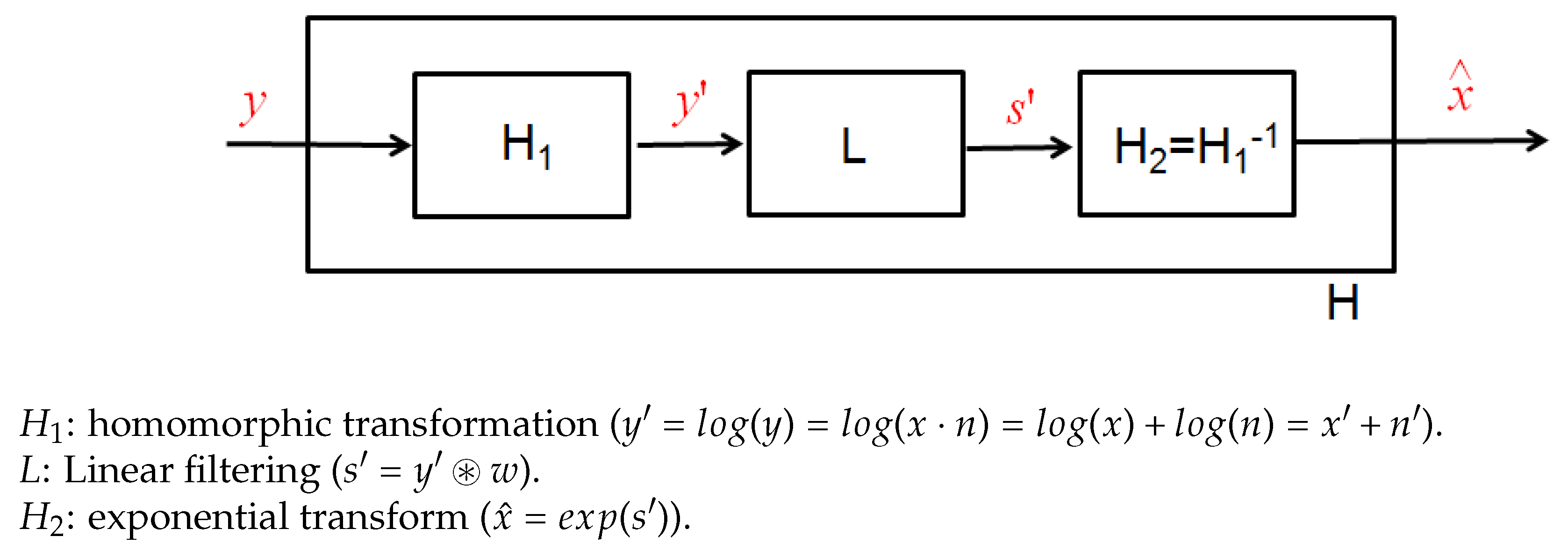
The signal y faces, at first, a homomorphic transformation, given by the logarithm function, which aims to convert the multiplicative speckle noise to an additive noise n′. Thus, we obtain a signal y′ defined as a summation between a noise-free signal x′ and a noise quantity n′ in the logarithmic domain. Next, y′ undergoes into a linear filtering L, described as a convolution with the Wiener kernel w, in order to achieve a filtered output s′. Finally, the latter returns to the initial domain using the exponential transform. The procedure is sketched in Figure 1.
Let us focus on the linear filtering step (L) in the frequency domain. In the filtering part, the Wiener kernel W is given by the following formula [10]:
where and denote respectively the power density spectrum of the image and noise. It should be noted that the dependence on the frequency variable has been neglected.
It is possible to retrieve the power spectrum of the noise for the implementation of WF, starting from its Auto-Correlation Function (ACF), as in [15]. Let us first consider the input noise of Equation (1). It follows an exponential distribution with mean and variance equal to one. After the transformation of , the noise changes its distribution, and its mean value becomes:
where is the Euler constant.
Exploiting the mean value given in Equation (3), it is possible to write down the auto-correlation function of the noise n′ as:
where the expectation is calculated using the joint Probability Distribution Function (PDF) of the noise sample in the pixels and .
By making the assumption of decorrelation between noise samples commonly adopted in the literature as for example in [2,6,7], the auto-correlation function becomes the Dirac delta function, whose value in zero is provided by:
The latter is calculated in closed form according to [16] and [17], and it represents the ACF of the noise after the transformation of operator . Since its mean is different from zero, in order to apply the WF, the contribution of the mean has to be eliminated. For this reason, the power spectrum of the noise n′ is calculated by applying a Fourier Transform (FT) to the ACF after removing the square mean of n′.
The power spectrum of the unknown image can be estimated using an iterative procedure as presented in [18].
Several more sophisticated techniques for the estimation of the power spectrum exist in the literature based on the -divergence, as [19], or based on the -divergence, as [20]. However, we considered a simple, yet effective approach in order to maintain a limited computational cost and speed up the algorithm.
Although the classical WF is a very fast filtering algorithm, it does not take into account the local characteristics of the image. Thus, the idea is to provide the local information to WF, keeping its good performances in terms of velocity. For that, we propose to modify the Wiener kernel by introducing the contextual information as:
where is a vector containing K linearly-spaced elements (or weights). The first value of the vector is assigned equal to one. It corresponds to the behavior of the classical WF. When increases, the filter tends to impose a stronger regularization. The idea is to link the values of the vector with the characteristics of the observed scene. It can be understood that large values of should correspond to homogeneous areas, and accordingly, the solution of WF in these areas is highly regularized. However, a slight regularization with small values of should be applied in the presence of edges. Moreover, the maximum value is a specific input parameter that must be tuned for each test case in order to reach the highest performance of the filter.
In this framework, it is mandatory to estimate for each pixel the contextual information in order to use the optimal value of . To this aim, we refer to the the Markovian Random Field theory (MRF). In particular, we adopt the Hyper-Parameter map . This map is used to provide an index of spatial correlation between neighboring pixels [21]. Hence, considering a local-central pixel p and 8-connexity neighboring system , the estimated hyper-parameter of this pixel can be calculated in closed form as:
where and denote respectively the values of the central pixel p and the neighboring pixel q. Clearly, and are not a priori known (incomplete data problem), and they need to be estimated. For this reason, we used the filtered solutions, as will be specified in the following.
Based on Equation (7), if a pixel belongs to a homogeneous area, then will be small. On the contrary, if a pixel belongs to an edge, will be large. Such a feature of can be used to improve the efficiency of WF. The map provides the information about the probability that two pixels have the same values.
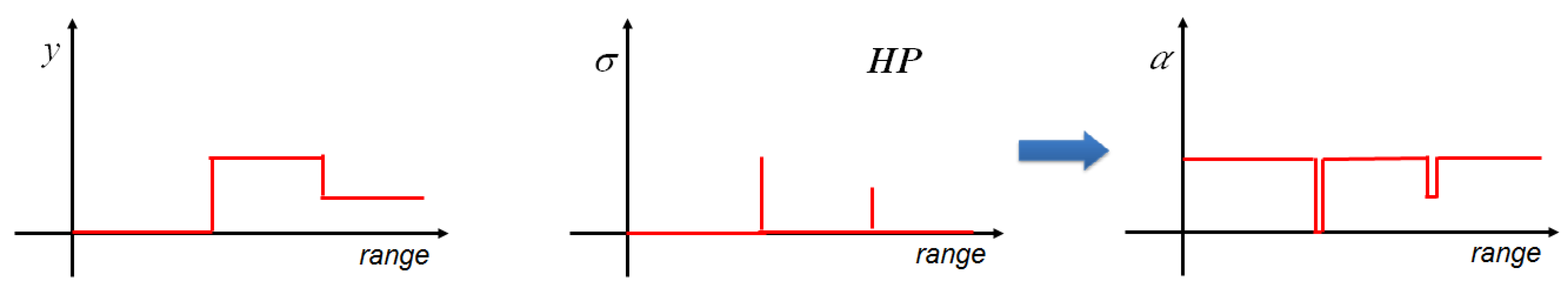
Once the hyper-parameter map is estimated, we define an , which is simply an inversion of the procedure. The parameter is given by the following formula:
Figure 2 illustrates both and processes for a given image profile characterized by flat areas (homogeneous areas) and edges. It can be seen that identifies those flat areas and those edges. From this, we can notice the process with the parameter, which is presented as an inversion of .
Hence, the provides for each pixel the optimal value of . In other words, it allows automatically selecting which is the best Wiener kernel to be applied for the specific pixel.
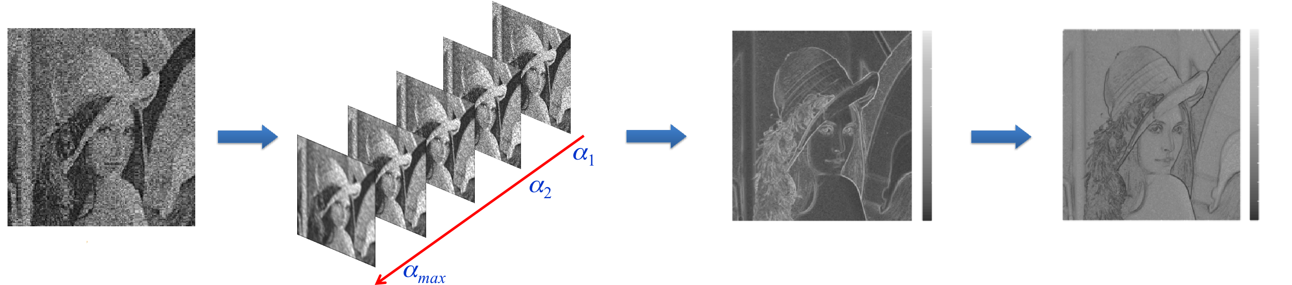
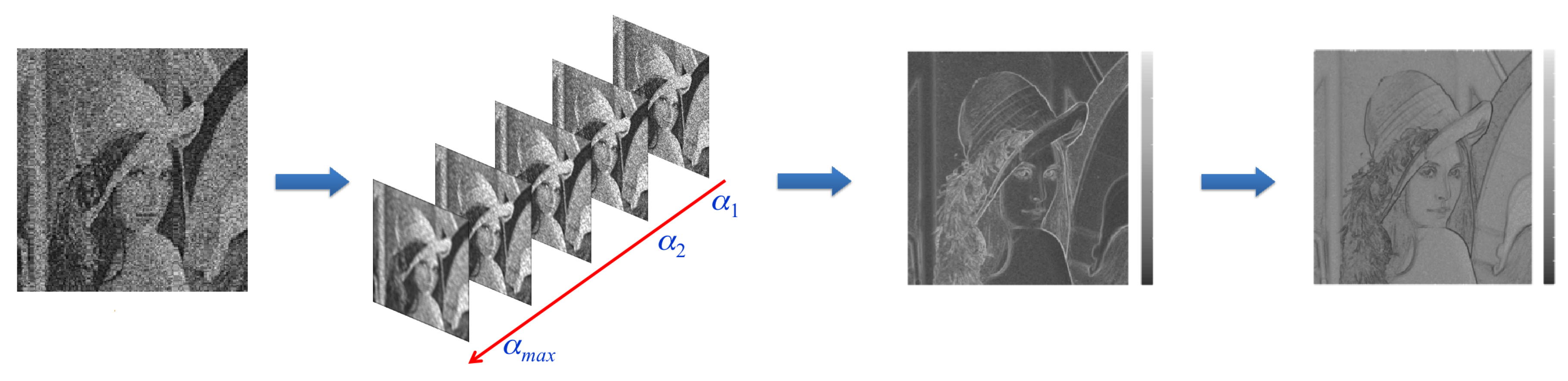
The processing steps of the proposed framework are illustrated in Figure 3 by referring to the well-known Lena picture. The image is affected by speckle noise. The first step involves the homomorphic transformation of the noisy image. Then, in the second step, we apply the Wiener filtering based on the modified kernel W′ using K different parameters of vector . Hence, this results in the generation of K filtered images. For each obtained filtered image, we estimate the using Equation (7), and we merge them by averaging them in order to achieve a single image. Then, the is obtained by inverting the merged output. Finally, we construct our final filtered output image by selecting each pixel from one of the K solutions based on the value presented in the .
Algorithm 1 describes the steps to proceed with our proposed methodology, called the Enhanced Wiener Filter (EWF) framework [22], starting from a noisy image and a specific input parameter, which is the maximum value of the vector . It should be noted that this latter must be tuned for each test case in order to reach the highest performance of the filter. The program was coded (Supplementary Materials) in MATLAB R2018a [23] environment, on an AMD Ryzen Threadripper 1950X 16-Core -GHz processor with Linux Debian as the operating system. The GPU used in this paper was a GeForce GTX 1080 Ti work station characterized by 12 GB of memory and 3584 CUDA Cores.
As is clear from Algorithm 1, the methodology was designed using simple functions well suited for GPU processing such as FFT and matrix products. This helps in maintaining the high efficiency. The idea is to provide the GPU large amounts of data and ask it to perform relatively simple operations. Other implementations could be adopted, but at the cost of the processing time.
| Algorithm 1 Enhanced Wiener filter framework. |
|
3. Experimental Results
This section aims to report the experimental results obtained by the proposed solution in comparison with some widely-used SAR despeckling approaches in the scientific community. The comparison algorithms are described in Section 3.1. Next, we refer to the adopted performance indicators used for quantitatively comparing the SAR filtering techniques that are reported in Section 3.2. Finally, we illustrate the obtained results for both simulated data (Section 3.3) and real SAR images (Section 3.4).
3.1. Comparison Algorithms
In order to evaluate the performance of our proposed solution, we compared it to some widely-known filters described as follows:
- Kuan filter [3]: a linear adaptive filter that applies the minimum Mean Squared Error (MSE) criteria to the model of interest after replacing it from a multiplicative noise model to a signal-dependent additive noise model. In this paper, we refer to a window size and a number of looks L equal to one.
- The iterative Probabilistic Patch-Based filter (PPB-it) [6]: a non-local approach that is presented as an improvement of the Weighted Maximum Likelihood Estimator (WMLE), which consists of refining iteratively the weights including patches from the estimate of the image parameters. Default parameters were proposed by the authors by proceeding with 25 iterations of the PPB filter, a window search size, and a patch size equal to . As for the alpha-quantile parameter and the filtering parameter T, they are respectively given as 0.92 and 0.2.
- Fast Adaptive Non-local SAR (FANS) filter [14]: an improved version of the SAR-BM3D algorithm that is based on both non-local filtering and wavelet-domain shrinkage concepts. This approach uses a variable-sized search area driven by the activity level of each patch and a probabilistic early termination approach that exploits speckle statistics in order to speed up block matching. Moreover, the use of look-up tables helps in further reducing the processing costs. Default parameters for FANS filter were used in this work as defined by the authors.
3.2. Performance Indexes
In the following section, the adopted indexes are illustrated. In particular, we used Pratt’s Figure Of Merit (FOM) [24] and the Structural Similarity (SSIM) index [25] in the case that a reference image was available. Moreover, we adopted two other parameters, properly defined in the case that the reference image was not available, which were: the -ratio index [26] and the Kullback–Leibler Distance or KL Divergence (KLD) [27,28].
More in detail, Pratt’s FOM was performed in order to quantify the filter’s capabilities on detecting the edges and preserving their shape. This measure was based on three issues, detection of all possible edges, localization (all edges should be placed in the correct location), and spurious response by avoiding false alarms [24].
The mathematical equation that describes FOM is given as follows:
where:
- and present respectively the number of actual and detected edges;
- denotes the Euclidean distance from the detected edge pixel to the nearest reference edge pixel;
- and is a scaling constant that modulates the cost of edge displacement.
The value of FOM parameter was between zero and one, and the higher was this index, the better was the filter at detecting and preserving the edges.
Concerning the SSIM index, it was performed in order to forecast the perceived quality of the digital data. In particular, it was used for measuring the similarity between two images, which depended on several factors including the luminance, the contrast, and the structure of the comparative data [25].
The measure of SSIM between a noise-free image x and an estimated restored image is calculated via the following equation:
where:
- and are the mean of x and , respectively;
- and are the standard deviation of x and , respectively;
- presents the covariance between x and ;
- and respect the default parameters defined by the authors in [25].
As for the -ratio index measure, it operates on the ratio image, which is achieved after realizing the point-to-point ratio between the noisy image and the filtered one, and measures the ability at removing speckle and remaining geometrical content within this ratio [26]. In fact, Equation (11) describes the -ratio estimator () as follows:
where:
- is the weighting coefficient fixed between zero and one;
- is the difference between the ENLof the noisy image and the ENL of the obtained ratio;
- denotes the residue of the speckle’s mean value;
- is an estimator responsible for measuring geometrical content.
Different from the other two previously-mentioned objective parameters, the -ratio index does not need a reference image. Moreover, the lower is , the better is the filter in terms of speckle noise reduction and edges’ detection and preservation.
Finally, the KLD measure is a natural non-symmetric distance function that measures the difference between two probability distributions p and q over the same variable x [27,28].
For continuous probability densities, the KLD, denoted , is defined as follows:
It is noted that does not need a reference image. This measure must be positive (). Moreover, the lower is the distance, the better is the filter at removing speckle noise from the data and preserving image details.
3.3. Simulated Data
In this part, we focus on evaluating, quantitatively and qualitatively, the performance of our proposed solution in comparison with the previously-defined approaches. For that, we illustrate the experimental results given in two simulated test cases that are defined respectively as: the squares test case (Section 3.3.1) and simulated Rome data (Section 3.3.2).
3.3.1. Squares
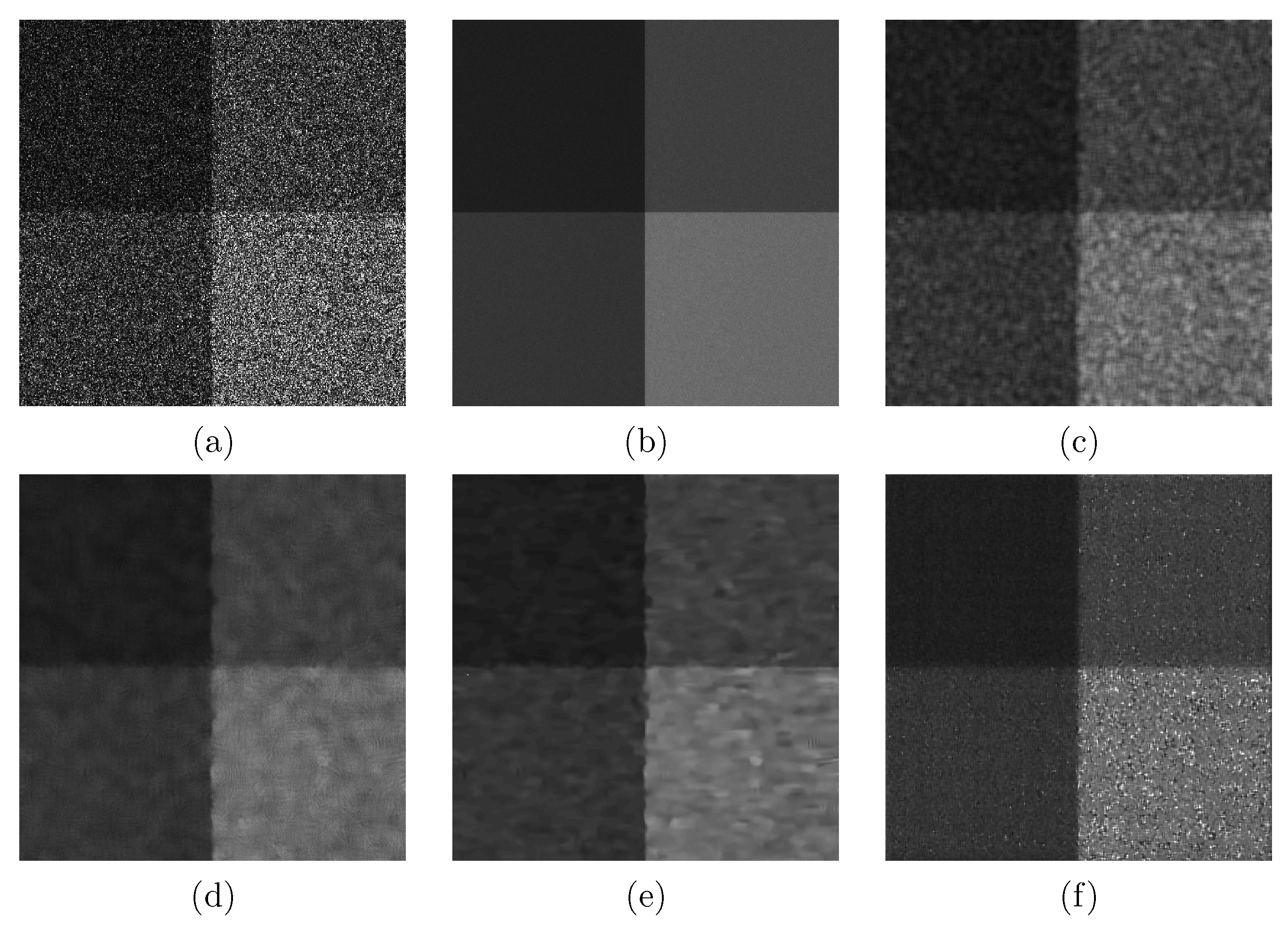
A single-look intensity SAR simulated dataset was considered for evaluating the capabilities of our developed technique in the squares test case. Indeed, these simulated data are composed of pixels and presented as four homogeneous areas with different gray-scale levels in the range. More details about the SAR simulated data are provided by the GRIPUnina database (www.grip.unina.it/research/80-sar-despeckling/85.html) [29].
Before presenting the graphical results, it should be noted that the size of the vector was set equal to 100 for all the test cases. Moreover, we should mention that we proceeded with tuning the input related to our developed method EWF in order to achieve a good trade-off between denoising the four different homogeneous areas on the one hand and preserving the shape of the edges separating these areas on the other hand. This condition is validated after referring to the numerical objective indicators. In fact, the optimal value was equal to 150 for this test case because this parameter provides a good trade-off between performance indicators given by the EWF solution.
Figure 4 reports the noisy SAR data, the 512-look reference, and the filtering outputs obtained after proceeding with the Kuan, PPB-it, and FANS filters and with our proposed technique EWF.
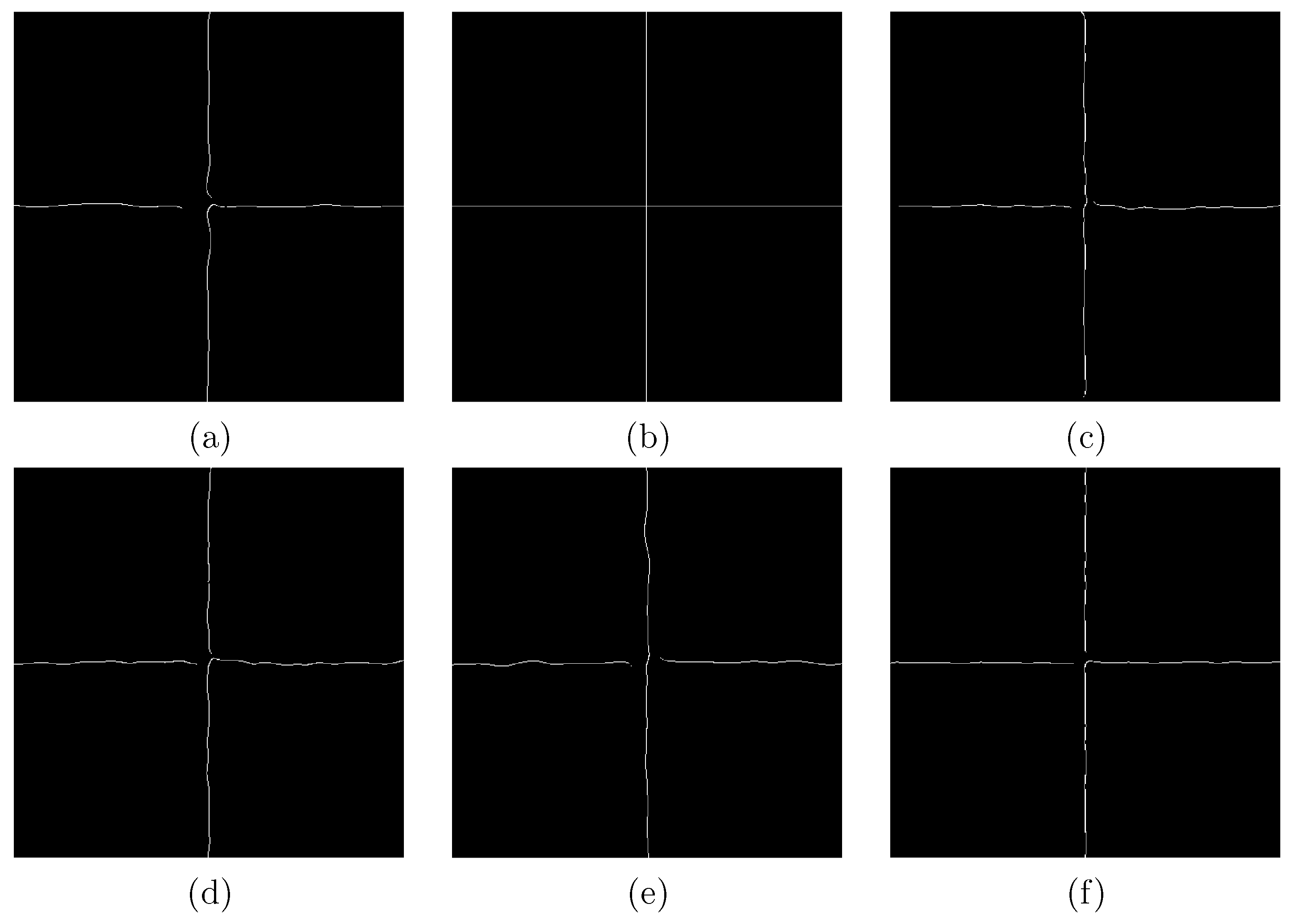
Besides, Figure 5 illustrates the edge maps obtained for the noisy SAR image, the clean reference, and the filtering techniques.
It is clear that the graphical results were not sufficient for a good assessment of a filter. For that, we refer to the following objective measures including FOM, SSIM, and the -ratio index together with the processing time.
We should mention that we did not take into consideration this KLD parameter for the squares simulated test case since this latter does not contain many structures. In fact, this index is very useful when many structures characterizing the image are presented.
Table 1 clarifies the values of these indexes given by the noisy SAR image, the clean one, and the different filtering techniques together with the processing time. It should be noted that we proceeded with the mean average of these parameters given after realizing eight iterations of processing. Moreover, we calculated for each filtering approach the measures related to the four homogeneous areas separately; then, we merged the obtained values for each area using the mean average process.
3.3.2. Rome
In this section, a single-look standard simulated image is considered. This dataset was used in order to analyze a remote sensing-like image and generated in intensity format according to the model of Equation (1), starting from the reference image. In particular, we first generated noise samples having an exponential distribution (Γ-distribution, with one look and in intensity format), and then, we multiplied it by the noise-free image.
To ensure a better comparison between the filters, objective assessment is required. In this case as well, we considered the FOM, SSIM, and -ratio parameters previously used in Section 3.3.1 in addition to integrating the KLD measure since the Rome test case contained many structures.
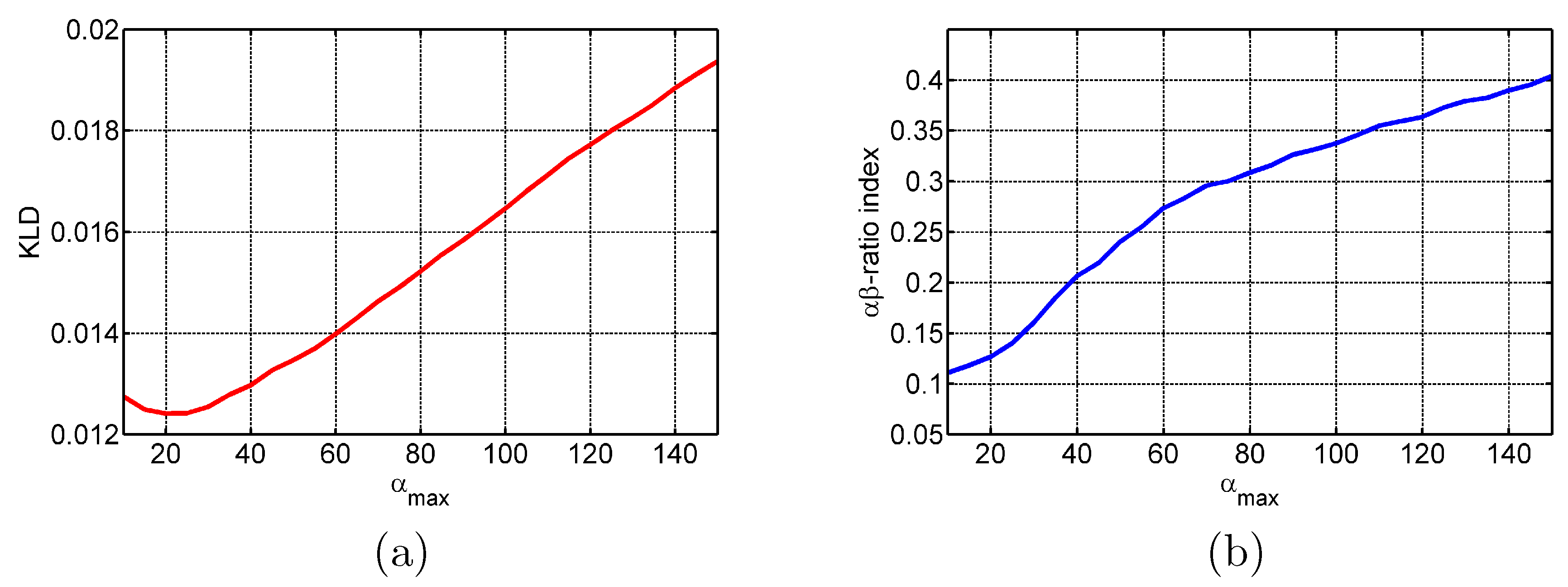
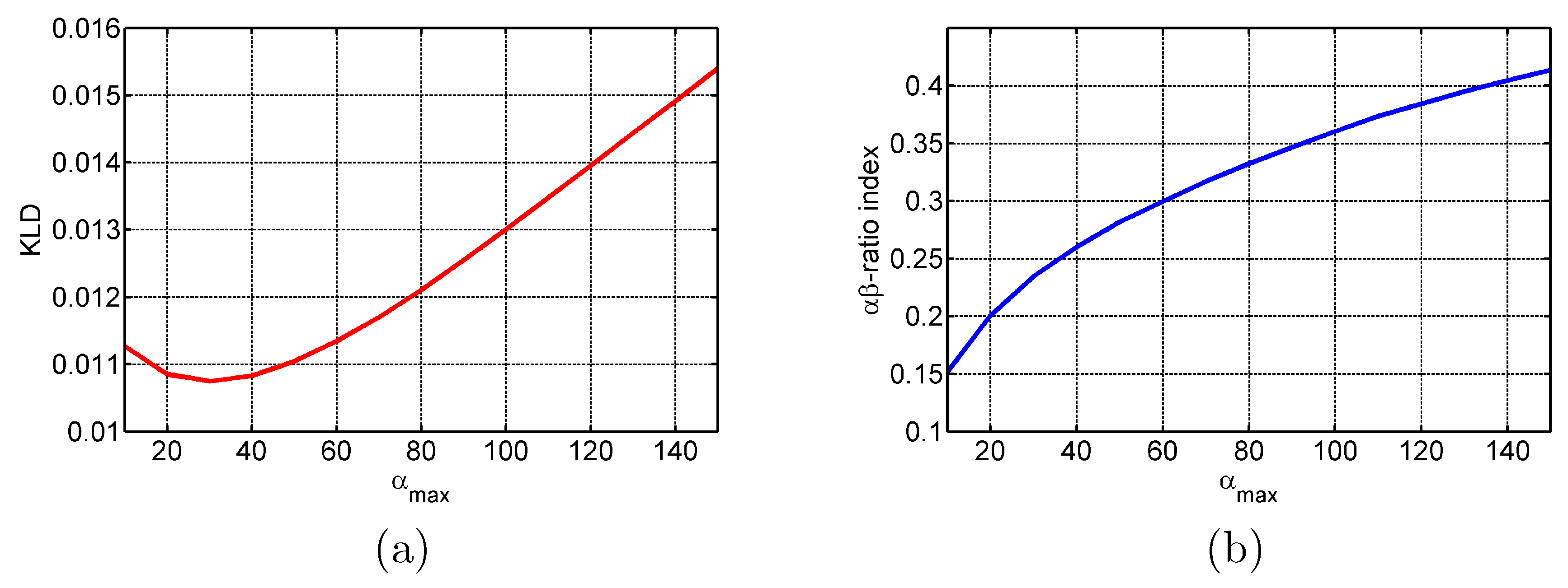
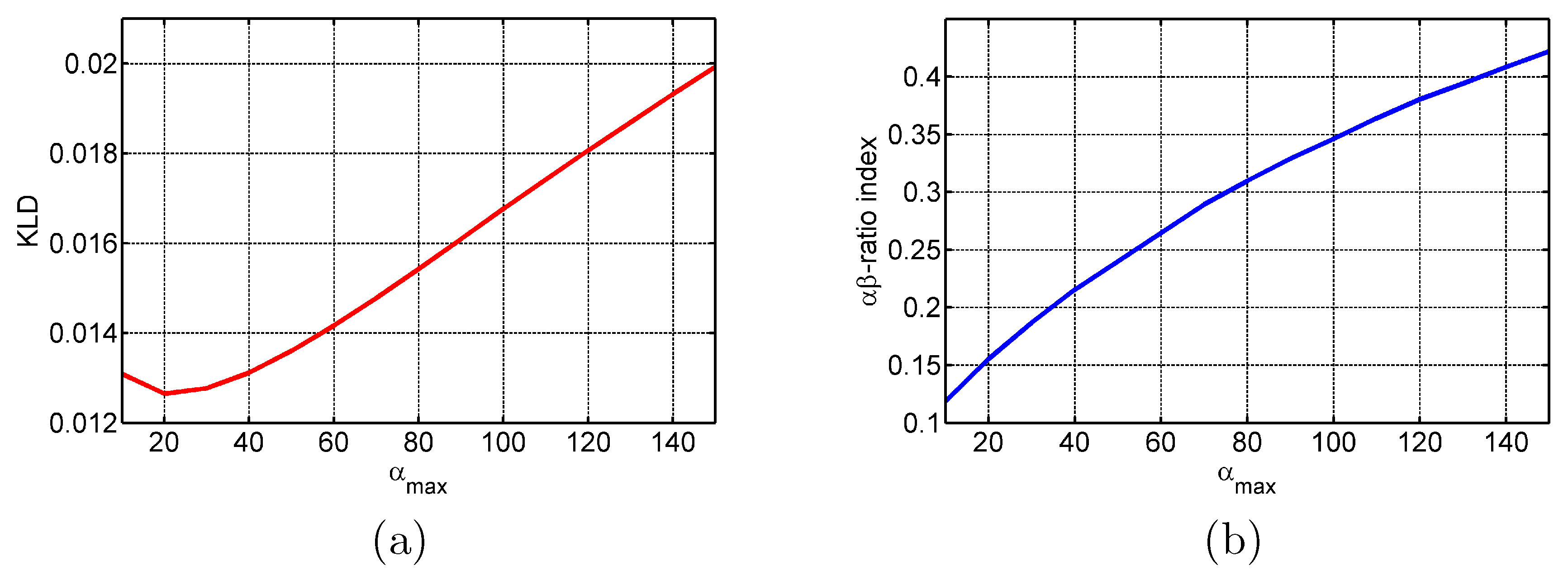
Next, we must select the suitable parameters for our developed solution in order to achieve its highest performance on despeckling simulated Rome data. For that, we detected the optimal that corresponded to the lowest KLD and -ratio index values. Therefore, Figure 6 reports the evolution of both the KLD and -ratio parameters as a function of input variation, passing from 10–150, related to our proposed algorithm EWF.
Considering Figure 6, we adopted an value equal to 20, which guaranteed the best value of KLD and, at the same time, a good value of the -ratio index. Therefore, we will assign this optimal value to the EWF technique for the graphical and the numerical results related to the Rome test case.
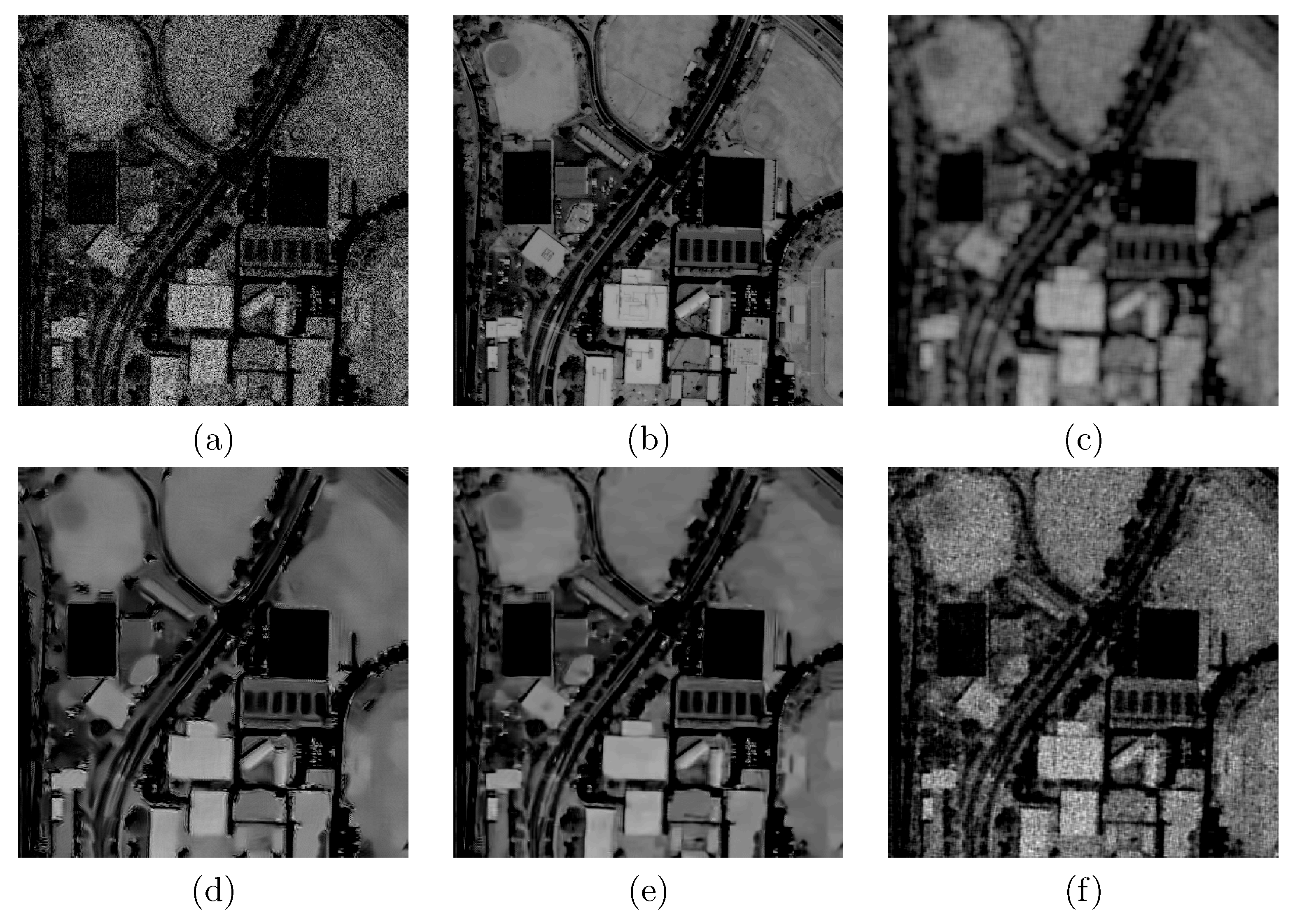
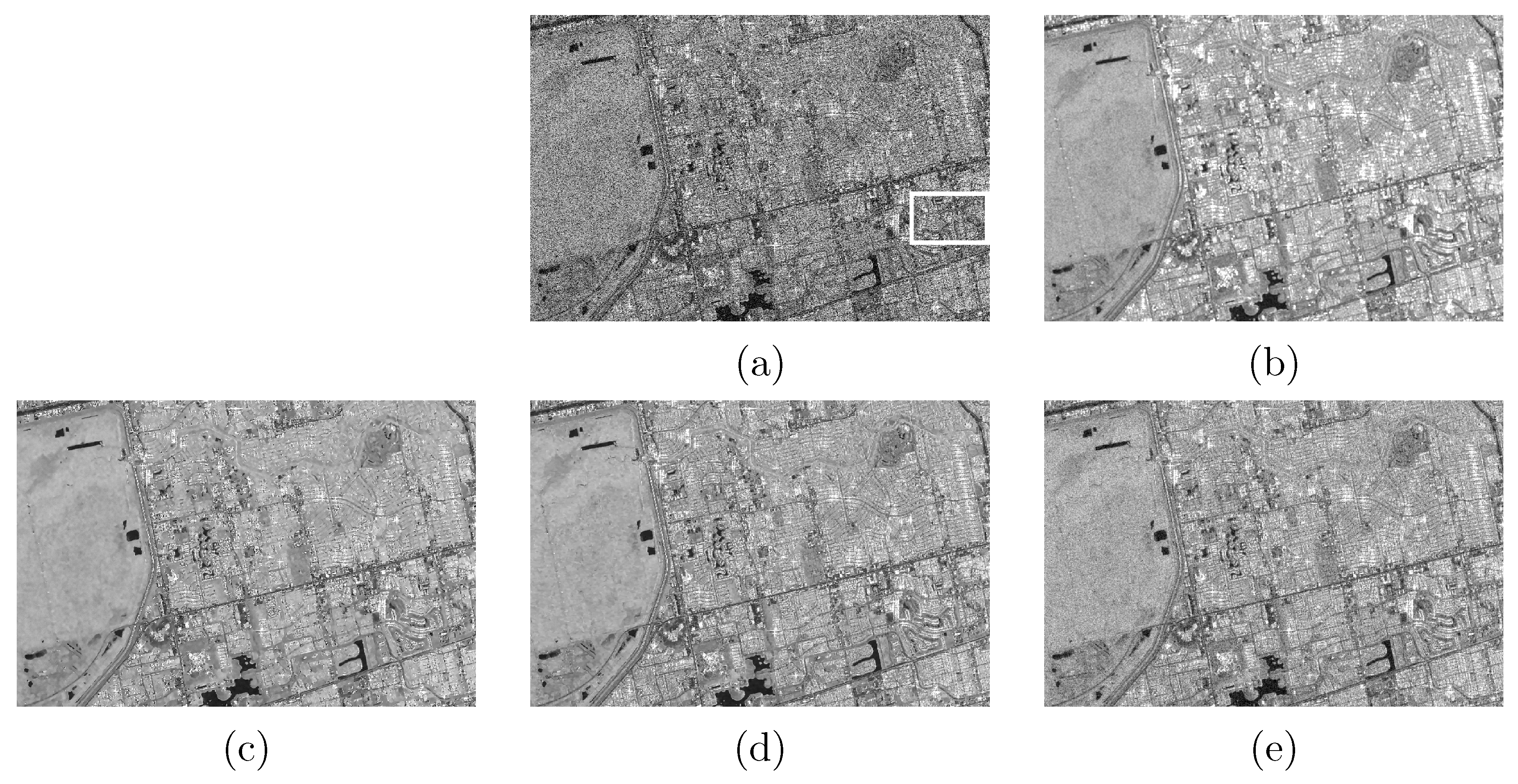
Hence, the comparison with the other filtering techniques related to the Rome test case is highlighted in Figure 7, Figure 8 and Figure 9. Figure 7 shows the test, reference, and filtered output images.
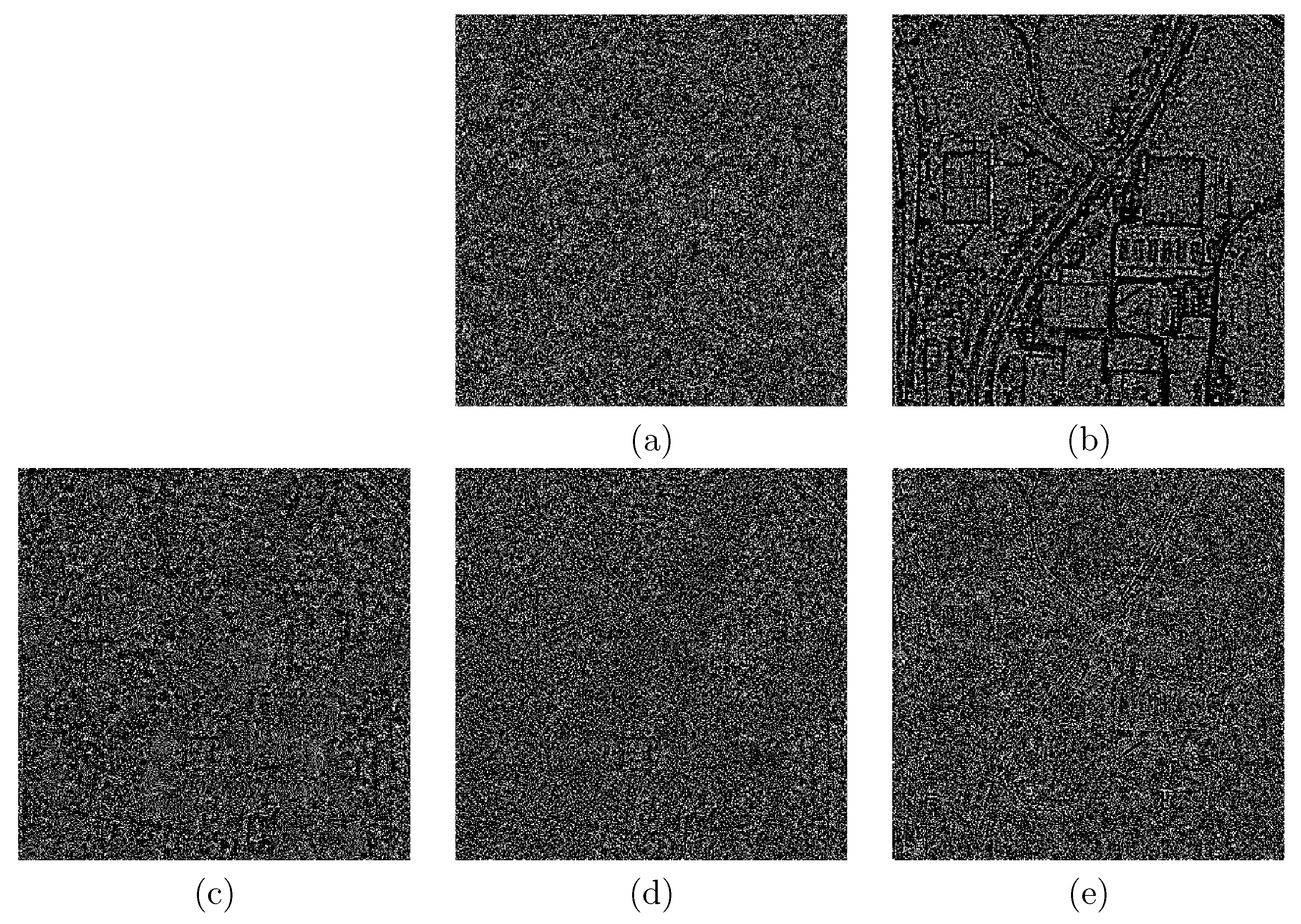
Figure 8 illustrates the ratio images obtained after proceeding with the filtering algorithms: Kuan, PPB-it, FANS, and our developed technique, together with the one related to the Rome clean reference.
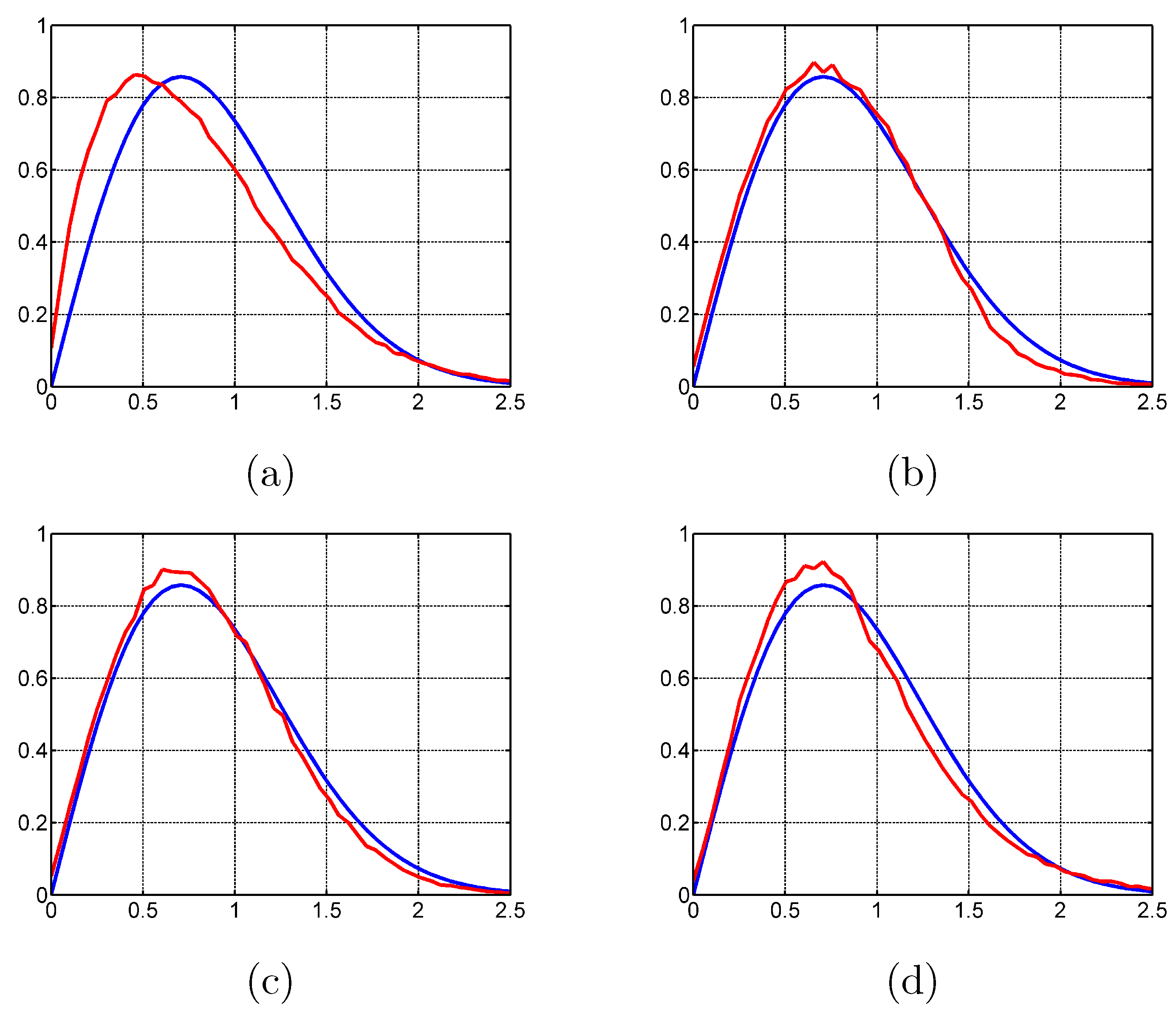
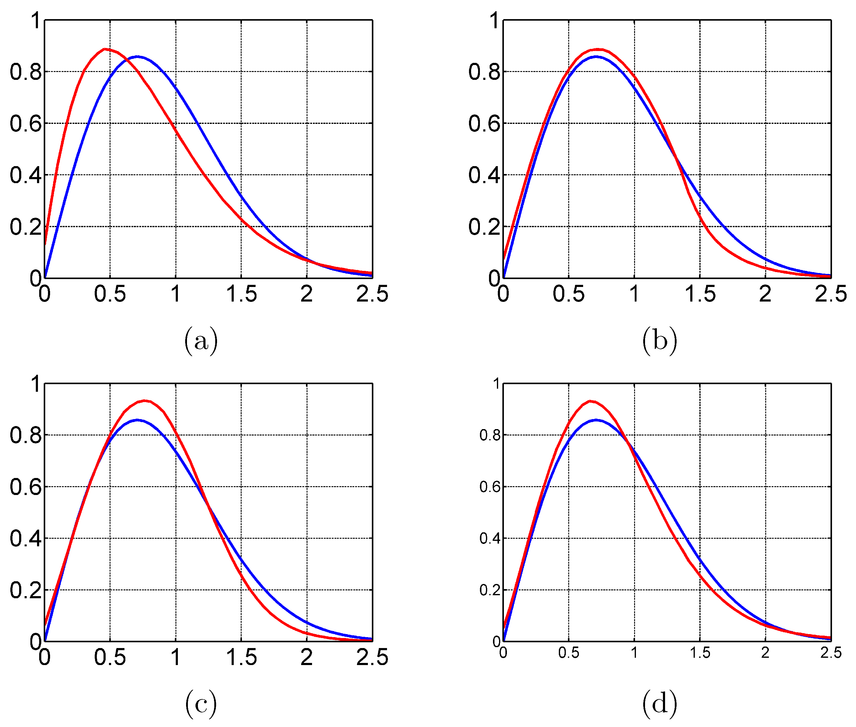
As for Figure 9, it presents the overlapping of the PDF of the expected speckle and of the PDF of the ratio images generated by the filtered outputs.
Numerical results are presented in Table 2, where the values of Pratt’s FOM, the SSIM parameter, the -ratio index, the KLD measure, and the processing time of each filter are shown.
3.4. SAR Real Data
In this Section, we present the quantitative and qualitative assessment of the filters’ capabilities on real SAR images. We compare our proposed solution EWF with the other filtering techniques cited in Section 3.1, on the basis of two Sentinel-1 datasets acquired with two different polarizations: Houston VV-pol data (Section 3.4.1) and Chicago HH-pol image (Section 3.4.2).
For both cases, we refer to the -ratio index and KLD parameter for objective assessment between the filtering algorithms’ capabilities on reducing speckle noise, since no reference is available.
3.4.1. Houston City
We present a C-Band Sentinel-1 SAR image, which is provided by the ESA database (https://scihub.copernicus.eu/dhus) and located in the United States of America, particularly in Houston between (, ) longitude and (, ) latitude. Moreover, this SAR image was acquired with a Stripmap (SM) acquisition mode, on 27 January 2019 from 12:31:06 UTC–12:31:30 UTC as an Intensity format Single-Look Complex (SLC) product in VV-polarization. We considered a patch of this SAR image.
An optimal value of for the Houston City SAR image has to be set in order to achieve its greatest capabilities on despeckling the scene and preserving the main characteristics of the image. Figure 10 illustrates the evolution of the KLD measure and -ratio index while varying the input, going from 10–150, given by our proposed solution EWF for the Houston test case.
Considering Figure 10, we adopted an value equal to 30, which guaranteed the best value of KLD and, at the same time, a good value of the -ratio index. Hence, we will make the graphical analysis and objective assessment related to the real Houston City SAR data for the EWF solution based on this value in comparison with the other filtering algorithms.
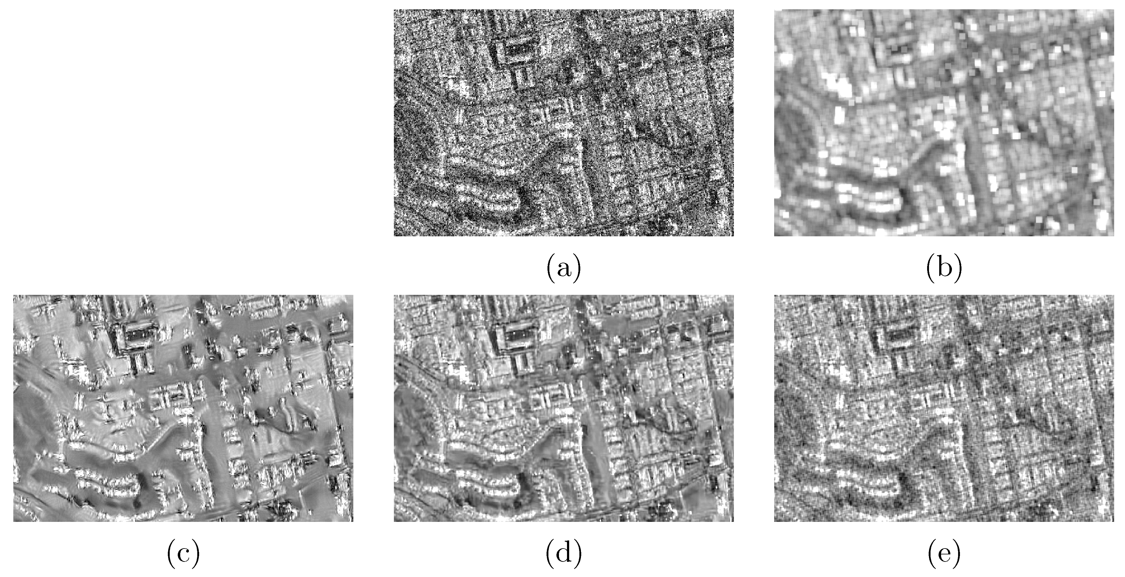
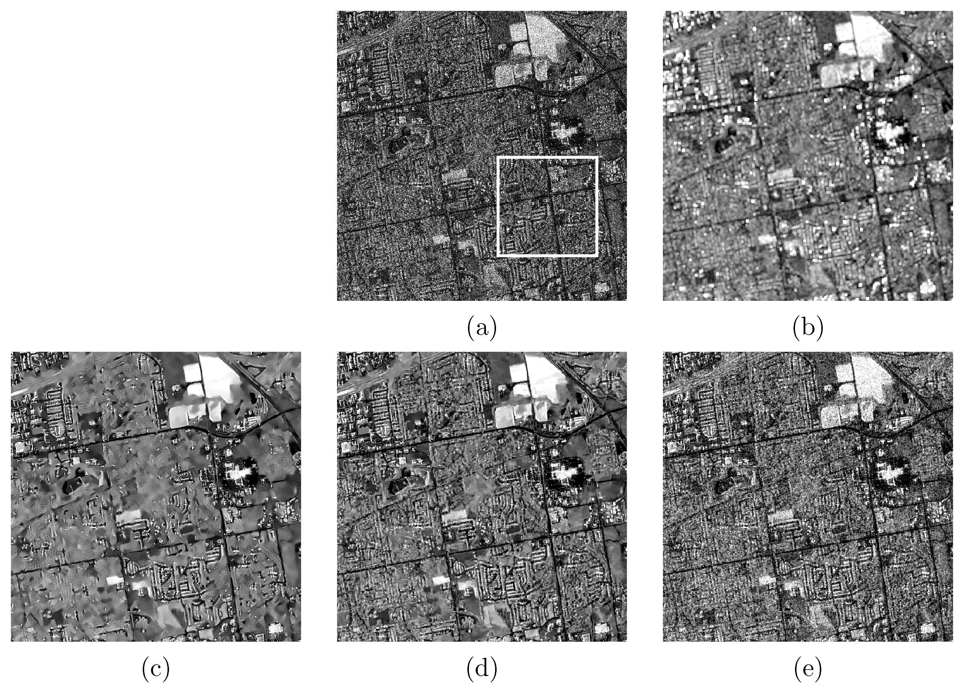
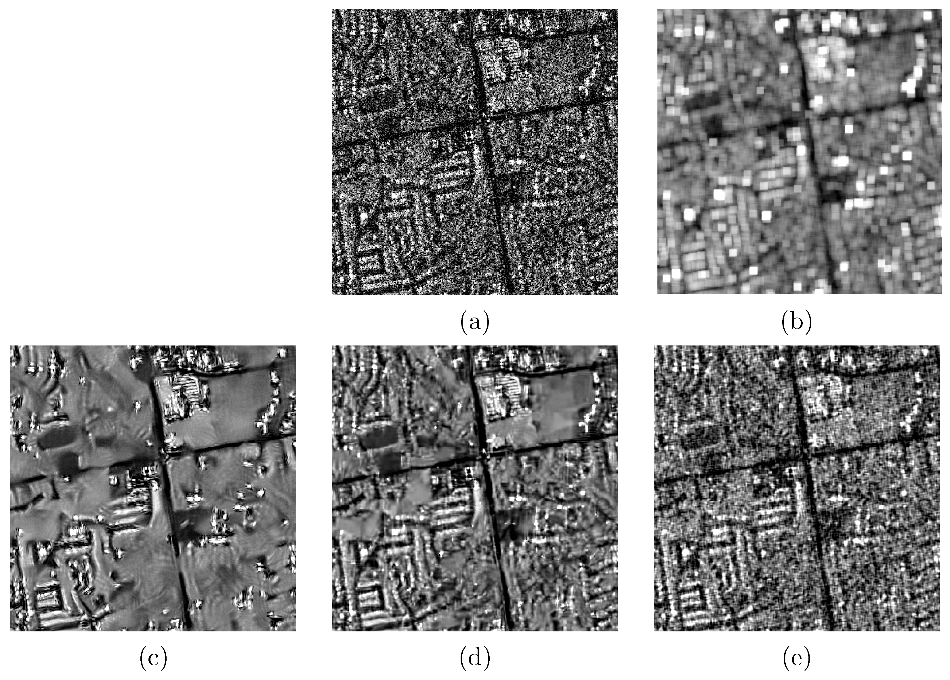
Figure 11 and Figure 12 report respectively the noisy SAR image and the zoom of a selected area (the white box) with a patch size equal to related to Houston City, together with the filtered outputs given after proceeding with: the Kuan, PPB-it, and FANS filters in comparison with our proposed solution. All the comparison filters were applied using the default configuration, provided by the authors as mentioned previously in Section 3.1.
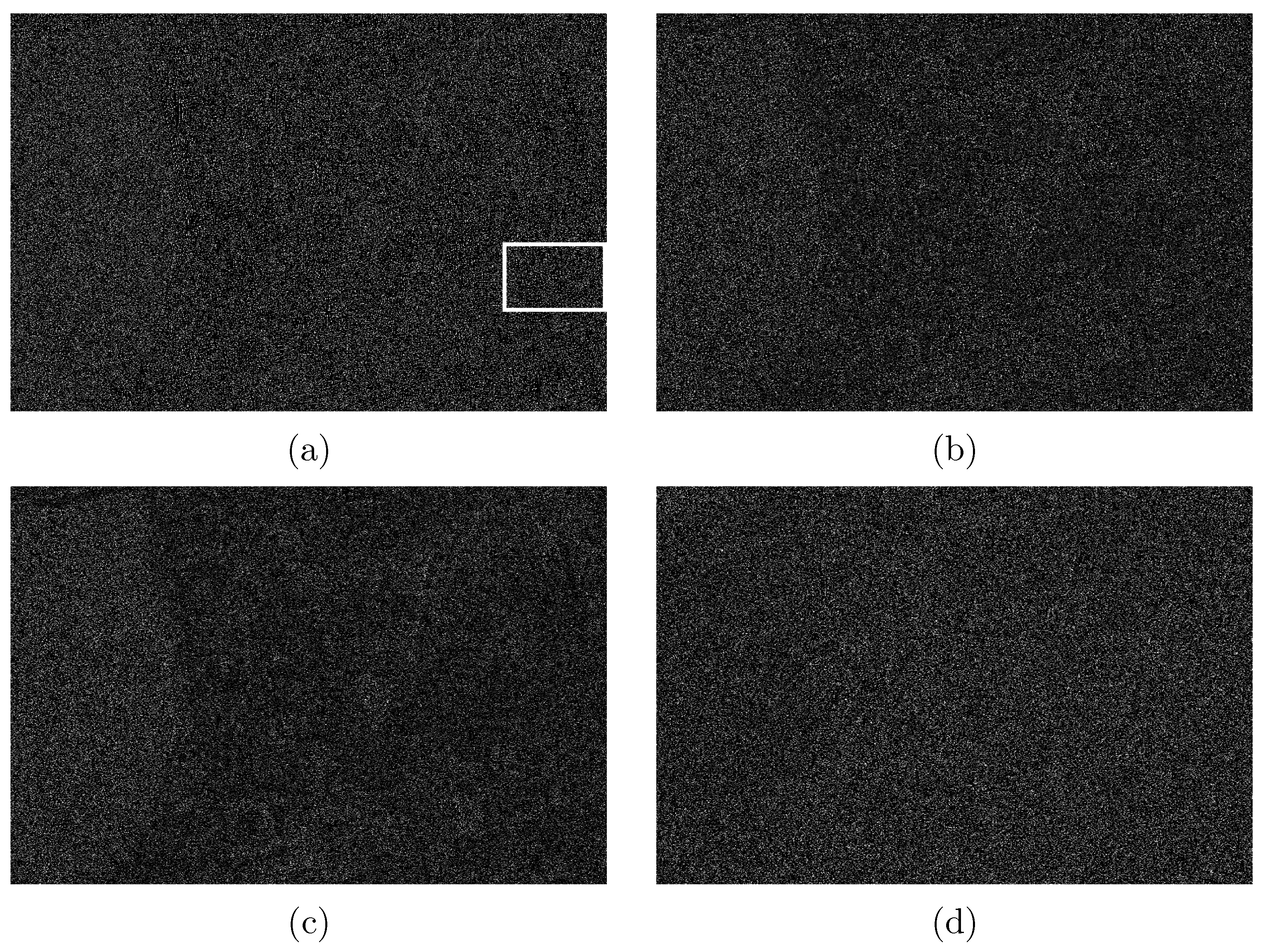
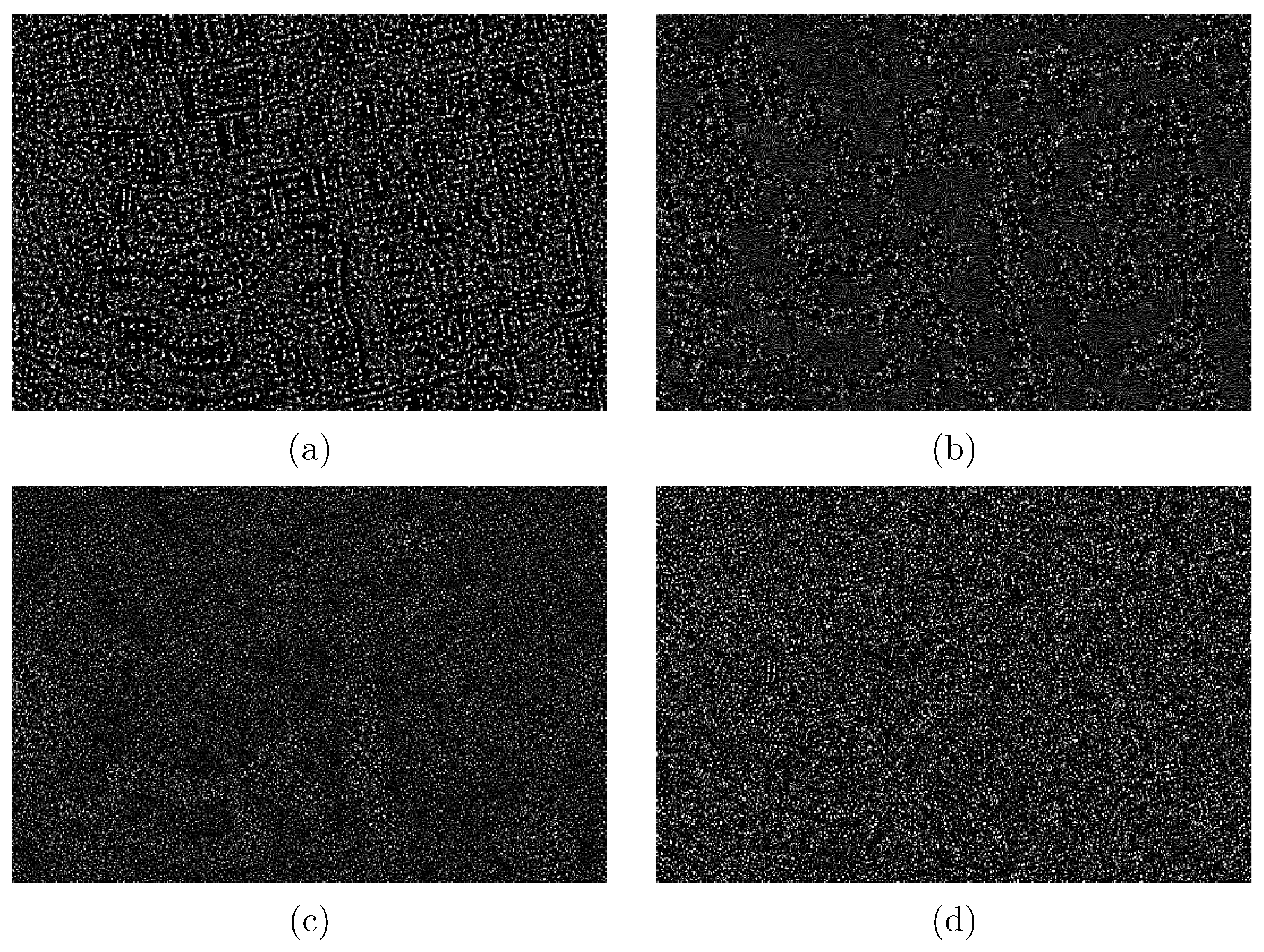
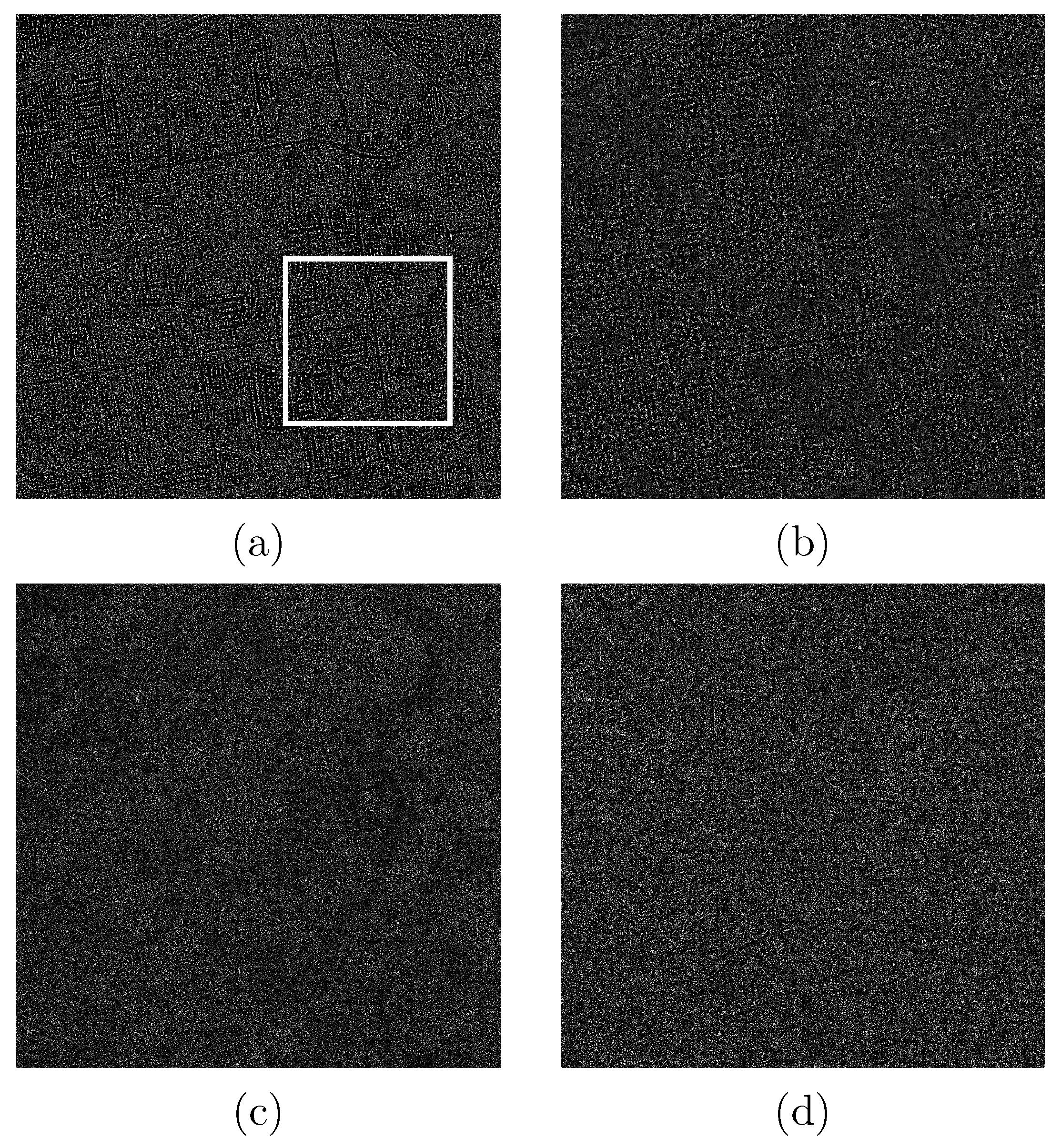
In Figure 13 and Figure 14, we report respectively the ratios of the restored images given after performing the selected filters related to the original Houston City SAR image and the selected patch area.
The overlapping of the PDF of the ratio of the restored output images in comparison with the one related to the expected speckle in amplitude format is sketched in Figure 15.
These graphical results were analytically evaluated by referring to both the -ratio index and KLD parameter, which are reported for each filtering algorithm and collected, together with the processing time, in Table 3.
3.4.2. Chicago City
The data used in this part were provided by a C-Band Sentinel-1 SAR satellite over the study region of the United States of America and particularly in Chicago City located between (, ) longitude and (, ) latitude. More in detail, these SAR data were acquired with SM acquisition mode, on 1 March 2018 from 11:54:53 UTC–11:55:16 UTC as an intensity format SLC product HH-polarization. We selected a patch from these data.
Once again, we needed to select the optimal value that maximized the performance of our developed solution. We illustrate the evolution of both KLD and -ratio indexes as a function of input, from 10–150, performed by EWF filtering algorithm for the Chicago City test case as highlighted in Figure 16.
Considering Figure 16: we adopted an value equal to 20, which guaranteed the best value of KLD and, at the same time, a good value of the -ratio index. For that, we will refer to this moderate value for this test case that gave the highest performance of our solution on removing speckle noise from the Chicago City SAR data.
As a visual comparison, we start by showing, in Figure 17, the noisy Sentinel-1 SAR image related to Chicago City together with the filtered output images obtained after performing: Kuan, PPB-it, FANS, and our proposed technique EWF. In this test case as well, the default configuration proposed by the authors was adopted for each comparison filter.
In Figure 18, a zoom with pixels, on a specific area in the Chicago City SAR data, is shown.
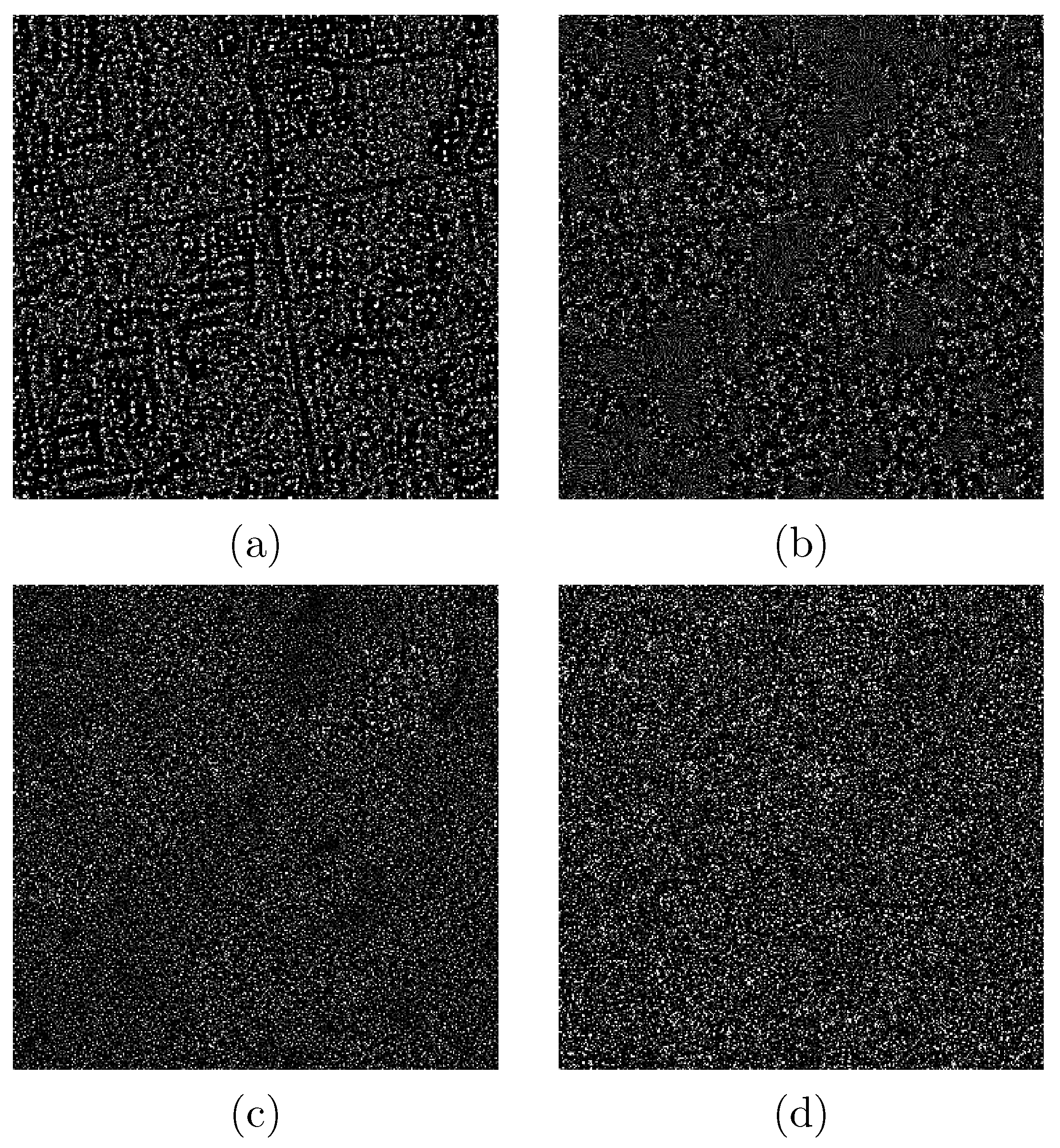
The ratio images obtained after proceeding with the filtering algorithms together with the zoom area are highlighted in Figure 19 and Figure 20.
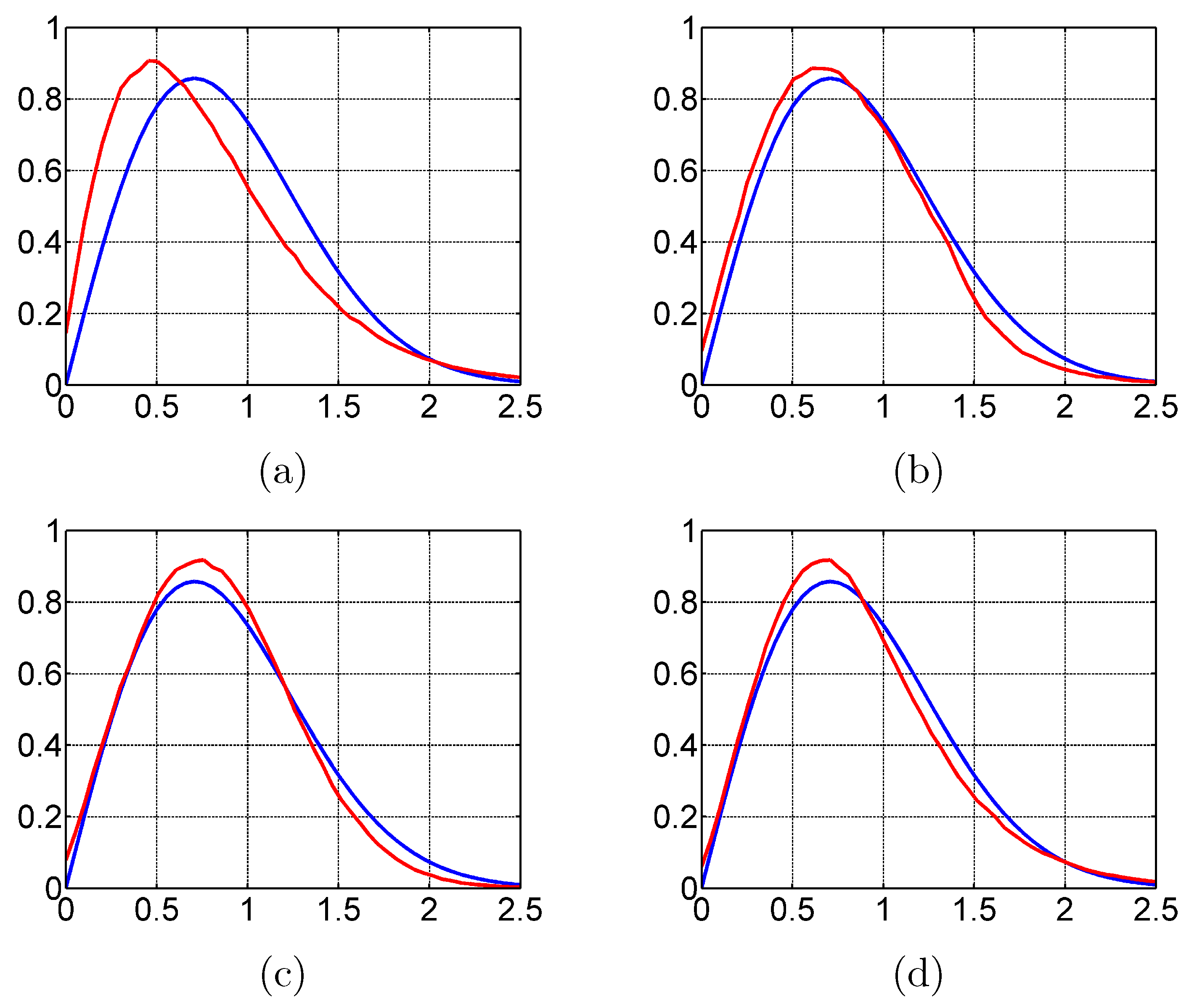
The overlapping of the expected speckle’s PDF and the PDF of the ratio images of the considered filters is presented in Figure 21.
It is relevant that visual inspection was not sufficient for a fair comparison between the filters’ capabilities. Therefore, Table 4 illustrates the values of the -ratio index and KLD measure together with the processing time performed by each filtering technique.
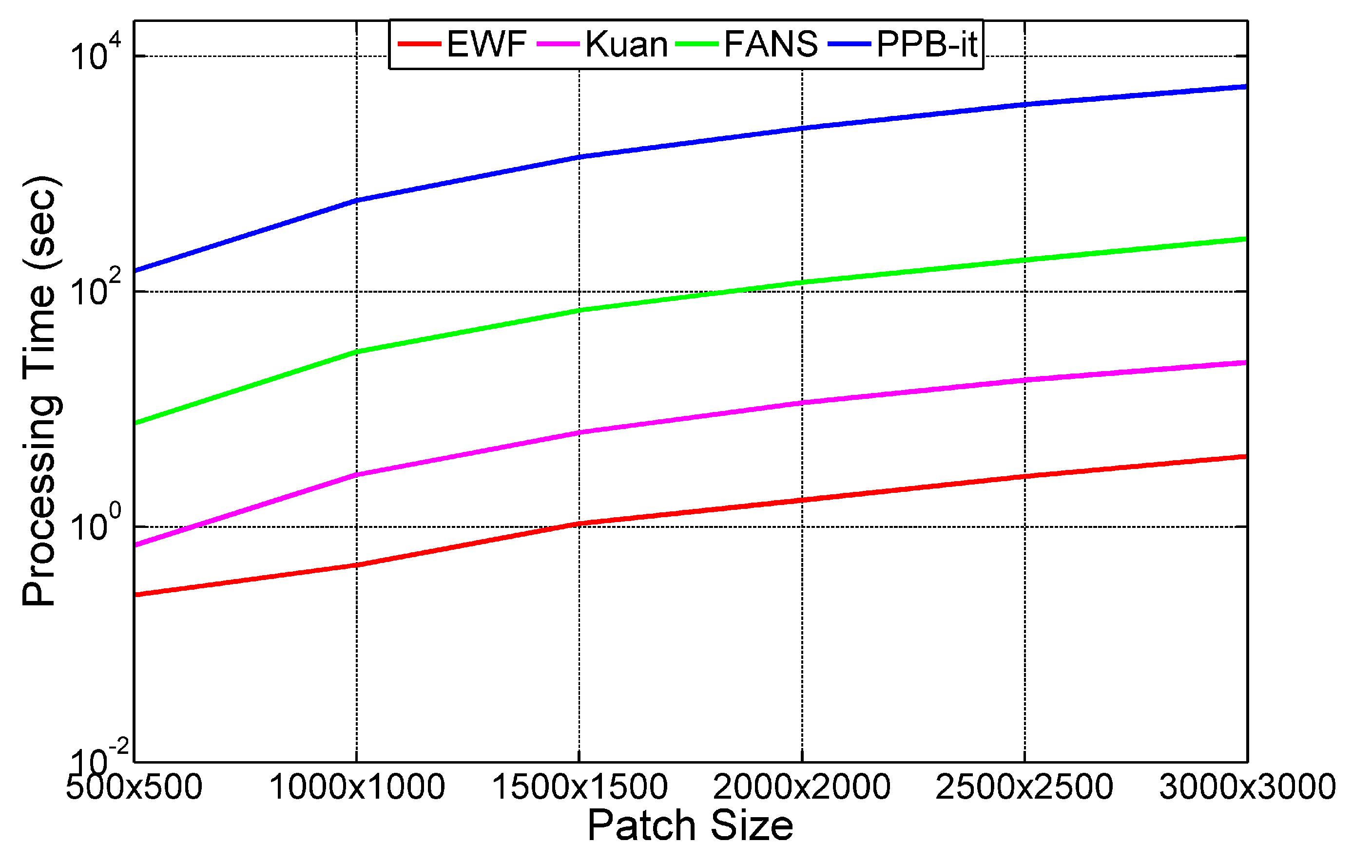
Finally, we focused on evaluating the processing time elapsed by all the filters used in this paper while varying the size of the Chicago City Sentinel-1 data. Hence, Table 5 reports the processing time of each filter while varying the Chicago City data patch size, passing from –. Figure 22 illustrates graphically the evolution of the processing time, in the logarithmic scale, performed by these filters as a function of patch size variation.
4. Discussion
In this section, we discuss the experimental results obtained by our proposed solution in comparison with the other filtering approaches for both simulated data (Section 4.1) and real SAR images (Section 4.2).
4.1. Simulated Data
This part aims to interpret the visual inspection and objective assessment related to the squares test case (Section 4.1.1) and the simulated Rome data (Section 4.1.2).
4.1.1. Squares
Based on the visual inspection between the filtered images and the clean reference one, shown in Figure 4, it is clear that both the PPB-it and FANS filters were characterized by the presence of some ghost artifacts that were generated due to their effort in recognizing structures. On the other hand, the Kuan filter and our proposed solution EWF illustrated their good capabilities at despeckling the squares scene. These results are confirmed in Table 1 by considering the -ratio performance indicator. In fact, the best value of was given by the Kuan filter, which was equal to 0.083, followed by our developed technique EWF (), which was better than non-local approaches including: the PPB-it and FANS filters.
As for the edge preservation, after referring to the edge maps given in Figure 5 by the restored images in comparison with the 512-look clean reference, we can notice that the PPB-it filter showed promising results on preserving edges separating the four different areas. This point is confirmed by both Pratt’s FOM measure and the SSIM index that are reported in Table 1, which concludes that PPB-it presented an outperformed solution in terms of edges and image detail preservation for the squares test case, as it illustrated the highest values of FOM and SSIM followed by the FANS filter and, then, by our developed solution EWF.
Finally, our proposed technique showed its interesting characteristic by providing a fast processing time in the GPU, equal to 0.25 s, better than all the filters presented in this paper. In fact, the processing time elapsed by EWF was three-times faster than the Kuan filter and approximately 20-times faster than the FANS algorithm.
4.1.2. Rome
In Figure 7 and Figure 8, visual comparison between the restored images together with the clean reference Rome data indicated that the Kuan filter did not perform well in terms of speckle noise reduction. Moreover, it caused smoothness and loss of the image edges and fine-details. Concerning the PPB-it and FANS filters, they performed well at removing the speckle noise. However, they presented some over-smoothed areas in their ratio images in comparison with the one obtained by the clean reference. In particular, the PPB-it filter showed the block effects technique. As for the FANS filter, it tried to produce some homogeneous regions in the data, while some parts were not homogeneous. Finally, our solution showed its good ability at despeckling the Rome scene with a homogeneous filtering shown in the ratio image despite the loss of of resolution and some edges.
In order to conclude the outperformed filter on removing speckle noise for the Rome simulated data, we considered the overlapping of the ratio images’ PDFs given by the filters together with the one related to the expected speckle in Figure 9. We notice that the FANS filter presented the best overlapping of PDF, followed by our technique EWF and by PPB-it. As for the Kuan filter, it showed the worst overlapping of PDF.
Hence, Table 2 confirms the visual assessment by illustrating FANS an outperformed solution for despeckling the Rome scene and preserving its main structure since it presented the highest values of the FOM and SSIM parameters and the lowest and KLD measures. The Kuan filter showed the worst values of FOM, SSIM, , and KLD presented. Our proposed technique EWF was more advanced than non-local approaches in terms of image detail preservation. However, it was slightly more advanced that the PPB-it filter for the -ratio index and presented the second highest value of the KLD measure (), better than the PPB-it and Kuan filters. Once again, EWF proved its good abilities of fast processing time and low memory occupation as it presented a processing time faster than both non-local filtering algorithms and the Kuan filter. In fact, our proposed solution was nearly 10-times faster than the FANS filter for the Rome test case.
4.2. Real SAR Data
Within this section, we discuss the quantitative and qualitative analysis obtained for the Houston City data (Section 4.2.1) and Chicago City SAR image (Section 4.2.2).
4.2.1. Houston City
Visual inspection allows the subjective assessment of the filters’ performance. We notice, in Figure 11 and Figure 12, that the Kuan filter caused smoothness of the data and blurred the SAR image edges and fine-details. Concerning the non-local approaches, it was clear that the PPB-it and FANS filters performed well at removing speckle noise with the edges and image fine-details’ preservation. As for our proposed method, it was characterized by a good speckle noise reduction of the scene with a considerable edges and image detail preservation.
In Figure 13 and Figure 14, we can see the presence of some structures in the ratio images provided by the Kuan filter, which confirms its incapability at preserving the main characteristics of SAR images. In addition to that, we noticed some over-smoothed regions in its ratio image, which concludes the adverse effects of spatial filtering on causing smoothness. As for the non-local filtering techniques, they preserved the main characteristics of SAR images as they did not present structures in their ratio images. However, these approaches were characterized by the absence of homogeneous filtering in some regions due to the block effect technique used by the PPB-it filter and the behavior of FANS filter at producing some homogeneous regions in the data, while some parts were not homogeneous, which led to an over-smoothing of these areas. Finally, our proposed technique was described by an homogeneous filtering for the whole of the Houston City SAR data with the absence of many edges and image details.
Next, we study the behavior of the PDF of the ratio images provided by the filtering approaches reported in Figure 15. The worst overlapping of the PDF was presented by the Kuan filter. Besides, our proposed method EWF illustrated the best overlapping followed by the PPB-it filter and the FANS filtering approach.
Finally, we conclude that the numerical results, reported in Table 3, confirmed the visual assessment. In fact, our solution presented the lowest KLD value (), followed by PPB-it (KLD in the order of 0.019) and, then, by the FANS filter (KLD over 0.022). Moreover, EWF was the second in terms of the -ratio index (), which was outperformed only by the FANS filter, which presented an value over 0.07. On the other hand, the Kuan filter showed the highest values of the KLD parameter and -ratio estimator, which confirms its incapability of providing good speckle noise reduction and image detail preservation. Finally, by referring to the last part of Table 3, the very interesting characteristic of our proposed method on real SAR data is shown, which is the fast processing time. Therefore, EWF was faster than all non-local approaches and approximately 10-times faster than the Kuan filter.
4.2.2. Chicago City
By visually inspecting the results between the filtering approaches for the Chicago City SAR image, presented in Figure 17 and Figure 18, it is evident that the Kuan filter over-smoothed the scene and blurred the main characteristics of the SAR data. Concerning non-local approaches, speckle noise was well removed. However, some homogeneous regions were figured in the restored images because PPB-it referred to the block effects technique and FANS pretended to over-smooth some regions after considering them as homogeneous parts. As for the proposed EWF, it showed its good ability at removing speckle noise from the Chicago City real SAR data while preserving the edges and the image fine-details.
By looking at the ratio images highlighted in Figure 19 and Figure 20, it is relevant that some image structures were clearly shown in the Kuan ratio-restored image. Once again, non-local techniques illustrated the absence of homogeneous filtering with some over-smoothed areas. In addition to that, the effectiveness of the proposed EWF was confirmed again. Details were well preserved; speckle was well removed; the ratio image was homogeneous for the whole of the SAR image.
To ensure a deep analysis in terms of speckle noise reduction capabilities, we focused on the overlapping of the PDF of the ratio images given by the filters in comparison to the theoretical one related to the expected speckle shown in Figure 21. EWF showed the best overlapping followed by the FANS, PPB-it, and then, by the Kuan spatial-based filtering technique.
Hence, the quantitative assessment reported in Table 4 summarizes the good performance of EWF in terms of speckle noise reduction. Our solution was characterized by the lowest KLD value over 0.013, which was better than the FANS and PPB-it filters, which presented KLDs respectively in the order of 0.018 and 0.02. Moreover, EWF presented the second highest value of , which was outperformed only by the FANS filter. The highest values of -ratio index and KLD measure were introduced by the Kuan filter, as it described the worst overlapping of the PDF. Once again, Table 4 highlights the main characteristic of EWF presented as the fast processing time on the real SAR data. In fact, our developed technique was nearly five-times faster than the Kuan filter and approximately 60-times faster than the FANS filter.
Finally, based on the fast processing time characteristic, we evaluated the graph highlighted in Figure 22, together with the values reported in Table 5, which describe the evolution of the processing time used during the filtering process of: Kuan, PPB-it, FANS, and EWF, while varying the Sentinel-1 SAR image patch size. By proceeding with this analysis, we can confirm that our proposed filtering algorithm EWF was always faster than both non-local approaches and the Kuan filter in terms of computational time in the processor with a large time difference achieved while increasing the patch size of the Chicago City Sentinel-1 SAR data. This point is very interesting for this study due to the dimensions characterizing Sentinel-1 data. In fact, EWF demonstrated that it was able of filtering a large Sentinel-1 SAR image in a reduced time, much less than all non-local approaches, with a good performance at removing speckle noise and a considerable edges and image detail preservation, better than the spatial approaches. It is important to highlight that the proposed GPU-based approach can guarantee a reduction of approximately 14-times the processing time compared to the same algorithm implemented on a CPU. This is due to the particular design and implementation of the algorithm using functions well suited for a GPU, such as the 2D FFT and IFFT.
5. Conclusions
SAR despeckling draw ever-increasing attention in the scientific literature, with several new techniques developed and proposed each time. Indeed, a new filtering algorithm processed in a GPU and based on modifying the kernel of Wiener filter was presented. The proposed test showed the interesting and promising capabilities of this denoising algorithm in both simulated and real SAR data. Concerning the simulated framework, based on the visual and numerical assessment, our proposed approach showed a good trade off between spatial techniques, including: the Kuan filter, and non-local approaches, for instance: the PPB-it and FANS filters, in both considered test cases with a considerable fast processing time. As for the real SAR data, Sentinel-1 SAR images were taken into consideration for this study. Visual inspection and numerical results proved that the algorithm turned out to be a good and almost unsupervised solution in terms of speckle noise reduction and image detail preservation, showing very effective results in processing time, which was faster than both the Kuan filter and non-local filtering techniques. Even in the case of large images, the filter was able to produce satisfying results within a very limited time. It turned out to be a very useful instrument for a fast despeckling of SAR images, mandatory for several applications. The proposed algorithm could suffer from some limitations in terms of memory requirements. However, the problem could be overcome by simply dividing the image into large patches, processing each, and then, merging the results. This procedure will still guarantee a processing time much smaller than the other approaches.
Future work includes extending this study to compare filters’ performances on other types of real SAR data including TerraSAR-X and CosmoSky-Med SAR images. Additionally, this work may be extended to deal with interferometric and polarimetric SAR data.
Supplementary Materials
The code is online available at the following link: https://github.com/gferraioli/GPUWienerDespeckling.git.
Author Contributions
Methodology, B.K., G.F., and G.S.; software, B.K.; supervision, V.P.; validation, B.K. and G.F.; writing, original draft, B.K.; writing, review and editing, G.F., V.P., and G.S.
Funding
The present work was partially funded by the University of Naples Parthenope, Italy, within the framework of the “Bando per il sostegno alla ricerca individuale per il triennio 2015–2017”.
Conflicts of Interest
The authors declare no conflict of interest.
Abbreviations
The following abbreviations are used in this manuscript:
| SAR | Synthetic Aperture Radar |
| EC | European Commission |
| ESA | European Space Agency |
| GPU | Graphics Processing Unit |
| ACF | Auto-Correlation Function |
| Probability Distribution Function | |
| FT | Fourier Transform |
| WF | Wiener Filter |
| EWF | Enhanced Wiener Filter |
| FANS | Fast Adaptive Non-local SAR |
| PPB-it | The iterative Probabilistic Patch-Based Filter |
| FOM | Pratt’s Figure Of Merit |
| SSIM | The Structural Similarity index |
| KLD | The Kullback–Leibler Distance |
References
- Ferretti, A.; Monti Guarnieri, A.; Prati, C.; Rocca, F.; Massonnet, D. InSAR Principles-Guidelines for SAR Interferometry Processing and Interpretation, Part A; ESA Publications: Noordwijk, The Netherlands, 2007. [Google Scholar]
- Argenti, F.; Lapini, A.; Bianchi, T.; Alparone, L. A tutorial on speckle reduction in synthetic aperture radar images. IEEE Geosci. Remote Sens. Mag. 2013, 1, 6–35. [Google Scholar] [CrossRef]
- Kuan, D.T.; Sawchuk, A.A.; Strand, T.C.; Chavel, P. Adaptive noise smoothing filter for images with signal-dependent noise. IEEE Trans. Pattern Anal. Mach. Intell. 1985, 7, 165–177. [Google Scholar] [CrossRef] [PubMed]
- Lee, J.S. Speckle analysis and smoothing of synthetic aperture radar images. Comput. Graph. Image Process. 1981, 17, 24–32. [Google Scholar] [CrossRef]
- Lopes, A.; Nezry, E.; Touzi, R.; Laur, H. Structure detection and statistical adaptive speckle filtering in SAR images. Int. J. Remote Sens. 1993, 14, 1735–1758. [Google Scholar] [CrossRef]
- Deledalle, C.A.; Denis, L.; Tupin, F. Iterative weighted maximum likelihood denoising with probabilistic patch-based weights. IEEE Trans. Image Process. 2009, 18, 2661. [Google Scholar] [CrossRef] [PubMed]
- Parrilli, S.; Poderico, M.; Angelino, C.; Verdoliva, L. A nonlocal SAR image denoising algorithm based on LLMMSE wavelet shrinkage. IEEE Trans. Geosci. Remote Sens. 2012, 50, 606–616. [Google Scholar] [CrossRef]
- Deledalle, C.A.; Denis, L.; Tupin, F.; Reigber, A.; Jäger, M. NL-SAR: A unified nonlocal framework for resolution-preserving (Pol)(In) SAR denoising. IEEE Trans. Geosci. Remote Sens. 2015, 53, 2021–2038. [Google Scholar] [CrossRef]
- Deledalle, C.A.; Denis, L.; Tabti, S.; Tupin, F. MuLoG, or How to apply Gaussian denoisers to multi-channel SAR speckle reduction? IEEE Trans. Image Process. 2017, 26, 4389–4403. [Google Scholar] [CrossRef] [PubMed]
- Portilla, J.; Strela, V.; Wainwright, M.J.; Simoncelli, E.P. Adaptive Wiener denoising using a Gaussian scale mixture model in the wavelet domain. In Proceedings of the 2001 International Conference on Image Processing (Cat. No.01CH37205), Thessaloniki, Greece, 7–10 October 2001; Volume 2, pp. 37–40. [Google Scholar]
- Zhang, Q.; Yuan, Q.; Li, J.; Yang, Z.; Ma, X. Learning a dilated residual network for SAR image despeckling. Remote Sens. 2018, 10, 196. [Google Scholar] [CrossRef]
- Vitale, S.; Ferraioli, G.; Pascazio, V. A New Ratio Image Based CNN Algorithm For SAR Despeckling. arXiv 2019, arXiv:1906.04111. [Google Scholar]
- Chierchia, G.; Cozzolino, D.; Poggi, G.; Verdoliva, L. SAR image despeckling through convolutional neural networks. In Proceedings of the 2017 IEEE International Geoscience and Remote Sensing Symposium (IGARSS), Fort Worth, TX, USA, 23–28 July 2017; pp. 5438–5441. [Google Scholar]
- Cozzolino, D.; Parrilli, S.; Scarpa, G.; Poggi, G.; Verdoliva, L. Fast adaptive nonlocal SAR despeckling. IEEE Geosci. Remote Sens. Lett. 2014, 11, 524–528. [Google Scholar] [CrossRef]
- Franceschetti, G.; Pascazio, V.; Schirinzi, G. Iterative homomorphic technique for speckle reduction in synthetic-aperture radar imaging. JOSA A 1995, 12, 686–694. [Google Scholar] [CrossRef]
- Gradshteyn, I.S.; Ryzhik, I.M. Table of Integrals, Series, and Products; Academic Press: San Diego, CA, USA, 2014. [Google Scholar]
- Baselice, F.; Ferraioli, F.; Ambrosanio, M.; Pascazio, V.; Schirinzi, G. Enhanced Wiener filter for ultrasound image restoration. Comput. Methods Programs Biomed. 2018, 153, 71–81. [Google Scholar] [CrossRef] [PubMed]
- Hillery, A.D.; Chin, R.T. Iterative Wiener filters for image restoration. IEEE Trans. Signal Process. 1991, 39, 1892–1899. [Google Scholar] [CrossRef]
- Eguchi, S.; Kano, Y. Robustifying Maximum Likelihood Estimation; Techical Report; Tokyo Institute of Statistical Mathematics: Tokyo, Japan, 2001. [Google Scholar]
- Zorzi, M. On the robustness of the Bayes and Wiener estimators under model uncertainty. Automatica 2017, 83, 133–140. [Google Scholar] [CrossRef] [Green Version]
- Ferraioli, G. Multichannel SAR Interferometry Based on Statistical Signal Processing. Ph.D. Thesis, Universita degli Studi di Napoli, Naples, Italy, 2008. [Google Scholar]
- Kanoun, B.; Ferraioli, G.; Pascazio, V.; Schirinzi, G. Fast Algorithm for Despeckling Sentinel-1 SAR Data. In Proceedings of the 12th European Conference on Synthetic Aperture Radar (EUSAR 2018), Aachen, Germany, 4–7 June 2018; pp. 1–5. [Google Scholar]
- MATLAB. Version 9.4.0.813654 (R2018a); The MathWorks Inc.: Natick, MA, USA, 2018. [Google Scholar]
- Pratt, W.K. Digital Image Processing, a Wiley-Interscience Publication; John Wiley and Sons: New York, NJ, USA, 1978. [Google Scholar]
- Wang, Z.; Bovik, A.C.; Sheikh, H.R.; Simoncelli, E.P. Image quality assessment: from error visibility to structural similarity. IEEE Trans. Image Process. 2004, 13, 600–612. [Google Scholar] [CrossRef] [PubMed]
- Gomez, L.; Buemi, M.E.; Jacobo-Berlles, J.C.; Mejail, M.E. A new image quality index for objectively evaluating despeckling filtering in SAR images. IEEE J. Sel. Top. Appl. Earth Obs. Remote Sens. 2016, 9, 1297–1307. [Google Scholar] [CrossRef]
- Kullback, S.; Leibler, R.A. On information and sufficiency. Ann. Math. Stat. 1951, 22, 79–86. [Google Scholar] [CrossRef]
- Ferraioli, G.; Pascazio, V.; Schirinzi, G. Ratio-Based Nonlocal Anisotropic Despeckling Approach for SAR Images. IEEE Trans. Geosci. Remote Sens. 2019, 1–14, early access. [Google Scholar] [CrossRef]
- Di Martino, G.; Poderico, M.; Poggi, G.; Riccio, D.; Verdoliva, L. Benchmarking framework for SAR despeckling. IEEE Trans. Geosci. Remote Sens. 2014, 52, 1596–1615. [Google Scholar] [CrossRef]
Figure 1.
Methodology schema.

Figure 2.
Example of and on an image profile: (left) noise-free one, (center) using , and (right) using .
Figure 2.
Example of and on an image profile: (left) noise-free one, (center) using , and (right) using .

Figure 3.
Example of the EWF contribution to the Lena picture. Moving from the left to the right: noisy image, Wiener filtering step providing K-solutions, , and .
Figure 3.
Example of the EWF contribution to the Lena picture. Moving from the left to the right: noisy image, Wiener filtering step providing K-solutions, , and .

Figure 4.
Squares test case: visual comparison between: (a) noisy SAR image, (b) clean, (c) Kuan, (d) PPB-it, (e) FANS, and (f) EWF.
Figure 4.
Squares test case: visual comparison between: (a) noisy SAR image, (b) clean, (c) Kuan, (d) PPB-it, (e) FANS, and (f) EWF.

Figure 5.
Squares test case: edge maps obtained for: (a) noisy SAR image, (b) clean, (c) Kuan, (d) PPB-it, (e) FANS, and (f) EWF.
Figure 5.
Squares test case: edge maps obtained for: (a) noisy SAR image, (b) clean, (c) Kuan, (d) PPB-it, (e) FANS, and (f) EWF.

Figure 6.
Rome test case: evolution of: (a) the KLD parameter and (b) the -ratio index, as a function of the variation for the EWF technique.
Figure 6.
Rome test case: evolution of: (a) the KLD parameter and (b) the -ratio index, as a function of the variation for the EWF technique.

Figure 7.
Rome test case: visual comparison between: (a) noisy image, (b) clean, (c) Kuan, (d) PPB-it, (e) FANS, and (f) EWF.
Figure 7.
Rome test case: visual comparison between: (a) noisy image, (b) clean, (c) Kuan, (d) PPB-it, (e) FANS, and (f) EWF.

Figure 8.
Rome test case: ratio images related to: (a) clean reference, (b) Kuan, (c) PPB-it, (d) FANS, and (e) EWF.
Figure 8.
Rome test case: ratio images related to: (a) clean reference, (b) Kuan, (c) PPB-it, (d) FANS, and (e) EWF.

Figure 9.
Rome test case: overlapping of the theoretical speckle PDF (blue line) and of the ratio images (red line) in amplitude format in the case of: (a) Kuan, (b) PPB-it, (c) FANS, and (d) EWF.
Figure 9.
Rome test case: overlapping of the theoretical speckle PDF (blue line) and of the ratio images (red line) in amplitude format in the case of: (a) Kuan, (b) PPB-it, (c) FANS, and (d) EWF.

Figure 10.
Houston test case. Evolution of: (a) the KLD parameter and (b) -ratio index, as a function of the variation for the EWF technique.
Figure 10.
Houston test case. Evolution of: (a) the KLD parameter and (b) -ratio index, as a function of the variation for the EWF technique.

Figure 11.
Houston test case: (a) Noisy SAR data, and restored images obtained using: (b) Kuan, (c) PPB-it, (d) FANS and (e) EWF.
Figure 11.
Houston test case: (a) Noisy SAR data, and restored images obtained using: (b) Kuan, (c) PPB-it, (d) FANS and (e) EWF.

Figure 12.
Houston test case. Zoom of a selected area obtained for: (a) noisy SAR data, (b) Kuan, (c) PPB-it, (d) FANS, and (e) EWF.
Figure 12.
Houston test case. Zoom of a selected area obtained for: (a) noisy SAR data, (b) Kuan, (c) PPB-it, (d) FANS, and (e) EWF.

Figure 13.
Houston test case. Ratio images obtained after proceeding with the filtering algorithms: (a) Kuan, (b) PPB-it, (c) FANS, and (d) EWF.
Figure 13.
Houston test case. Ratio images obtained after proceeding with the filtering algorithms: (a) Kuan, (b) PPB-it, (c) FANS, and (d) EWF.

Figure 14.
Houston test case. Zoom of the selected area ratio images obtained after proceeding with the filtering algorithms: (a) Kuan, (b) PPB-it, (c) FANS, and (d) EWF.
Figure 14.
Houston test case. Zoom of the selected area ratio images obtained after proceeding with the filtering algorithms: (a) Kuan, (b) PPB-it, (c) FANS, and (d) EWF.

Figure 15.
Houston test case. Overlapping of the theoretical speckle PDF (blue line) and the one related to ratio images in amplitude format in the case of: (a) Kuan, (b) PPB-it, (c) FANS, and (d) EWF.
Figure 15.
Houston test case. Overlapping of the theoretical speckle PDF (blue line) and the one related to ratio images in amplitude format in the case of: (a) Kuan, (b) PPB-it, (c) FANS, and (d) EWF.

Figure 16.
Chicago test case. Evolution of: (a) the KLD measure and (b) -ratio index, as a function of the variation for the EWF technique.
Figure 16.
Chicago test case. Evolution of: (a) the KLD measure and (b) -ratio index, as a function of the variation for the EWF technique.

Figure 17.
Chicago test case: (a) noisy SAR data and restored images obtained using: (b) Kuan, (c) PPB-it, (d) FANS, and (e) EWF.
Figure 17.
Chicago test case: (a) noisy SAR data and restored images obtained using: (b) Kuan, (c) PPB-it, (d) FANS, and (e) EWF.

Figure 18.
Chicago test case. Zoom of a selected area obtained for: (a) Noisy SAR data, (b) Kuan, (c) PPB-it, (d) FANS, and (e) EWF.
Figure 18.
Chicago test case. Zoom of a selected area obtained for: (a) Noisy SAR data, (b) Kuan, (c) PPB-it, (d) FANS, and (e) EWF.

Figure 19.
Chicago test case. Ratio images obtained after proceeding with the filtering algorithms: (a) Kuan, (b) PPB-it, (c) FANS, and (d) EWF.
Figure 19.
Chicago test case. Ratio images obtained after proceeding with the filtering algorithms: (a) Kuan, (b) PPB-it, (c) FANS, and (d) EWF.

Figure 20.
Chicago test case. Zoom of ratio images obtained after proceeding with the filtering algorithms: (a) Kuan, (b) PPB-it, (c) FANS, and (d) EWF.
Figure 20.
Chicago test case. Zoom of ratio images obtained after proceeding with the filtering algorithms: (a) Kuan, (b) PPB-it, (c) FANS, and (d) EWF.

Figure 21.
Chicago test case. Overlapping of the theoretical speckle PDF (blue line) and the one related to ratio images in amplitude format in the case of: (a) Kuan, (b) PPB-it, (c) FANS, and (d) EWF.
Figure 21.
Chicago test case. Overlapping of the theoretical speckle PDF (blue line) and the one related to ratio images in amplitude format in the case of: (a) Kuan, (b) PPB-it, (c) FANS, and (d) EWF.

Figure 22.
Processing time evolution (in logarithmic scale) performed by the filtering algorithms as a function of patch size variation related to the Chicago City Sentinel-1 SAR image.
Figure 22.
Processing time evolution (in logarithmic scale) performed by the filtering algorithms as a function of patch size variation related to the Chicago City Sentinel-1 SAR image.


Table 1.
Measures for squares.
| FOM | SSIM | Proc.Time (s) | ||
|---|---|---|---|---|
| Clean | 0.993 | 1 | 0 | - |
| Noisy | 0.792 | - | - | - |
| Kuan | 0.798 | 0.9989 | 0.083 | 0.75 |
| PPB-it | 0.828 | 0.9996 | 0.242 | 154.31 |
| FANS | 0.802 | 0.9994 | 0.221 | 5.06 |
| EWF | 0.808 | 0.999 | 0.212 | 0.25 |
Table 2.
Measures for Rome.
| FOM | SSIM | KLD () | Proc. Time (s) | ||
|---|---|---|---|---|---|
| Clean | 1 | 1 | 0 | 0.518 | - |
| Kuan | 0.467 | 0.504 | 0.558 | 4.27 | 0.49 |
| PPB-it | 0.667 | 0.633 | 0.104 | 1.48 | 95.82 |
| FANS | 0.732 | 0.707 | 0.02 | 0.908 | 4.18 |
| EWF | 0.594 | 0.544 | 0.127 | 1.24 | 0.39 |
Table 3.
Measures for the real Houston City SAR data.
| KLD (×) | Proc. Time (s) | ||
|---|---|---|---|
| Kuan | 0.652 | 5.47 | 20.63 |
| PPB-it | 0.234 | 1.91 | 4080.76 |
| FANS | 0.072 | 2.23 | 192.85 |
| EWF | 0.225 | 1.08 | 2.61 |
Table 4.
Measures for the real Chicago City SAR data.
| KLD () | Proc. Time (s) | ||
|---|---|---|---|
| Kuan | 0.681 | 6.26 | 2.77 |
| PPB-it | 0.272 | 1.96 | 593.76 |
| FANS | 0.073 | 1.84 | 30.73 |
| EWF | 0.155 | 1.27 | 0.47 |
Table 5.
Processing time elapsed by the filters (in seconds) while varying the Chicago City data patch size.
Table 5.
Processing time elapsed by the filters (in seconds) while varying the Chicago City data patch size.
| Kuan | 0.69 | 2.77 | 6.33 | 11.31 | 17.68 | 24.99 |
| PPB-it | 148.87 | 593.76 | 1386.44 | 2432.31 | 3875.02 | 5520.53 |
| FANS | 7.56 | 30.73 | 69.19 | 119.43 | 185.04 | 280.33 |
| EWF | 0.26 | 0.47 | 1.07 | 1.68 | 2.69 | 3.98 |
© 2019 by the authors. Licensee MDPI, Basel, Switzerland. This article is an open access article distributed under the terms and conditions of the Creative Commons Attribution (CC BY) license (http://creativecommons.org/licenses/by/4.0/).
Share and Cite
MDPI and ACS Style
Kanoun, B.; Ferraioli, G.; Pascazio, V.; Schirinzi, G. Fast GPU-Based Enhanced Wiener Filter for Despeckling SAR Data. Remote Sens. 2019, 11, 1473. https://doi.org/10.3390/rs11121473
AMA Style
Kanoun B, Ferraioli G, Pascazio V, Schirinzi G. Fast GPU-Based Enhanced Wiener Filter for Despeckling SAR Data. Remote Sensing. 2019; 11(12):1473. https://doi.org/10.3390/rs11121473
Chicago/Turabian StyleKanoun, Bilel, Giampaolo Ferraioli, Vito Pascazio, and Gilda Schirinzi. 2019. "Fast GPU-Based Enhanced Wiener Filter for Despeckling SAR Data" Remote Sensing 11, no. 12: 1473. https://doi.org/10.3390/rs11121473
Note that from the first issue of 2016, this journal uses article numbers instead of page numbers. See further details here.