Mapping Urban Areas Using a Combination of Remote Sensing and Geolocation Data

1
Jiangsu Provincial Key Laboratory of Geographic Information Science and Technology, Nanjing University, Nanjing 210093, China
2
Department of Geographic Information Science, Nanjing University, Nanjing 210093, China
3
Fenner School of Environment and Society, Australian National University, Canberra, ACT 2601, Australia
4
Collaborative Innovation Center for the South Sea Studies, Nanjing University, Nanjing 210093, China
*
Author to whom correspondence should be addressed.
Remote Sens. 2019, 11(12), 1470; https://doi.org/10.3390/rs11121470
Submission received: 23 May 2019
/
Revised: 14 June 2019
/
Accepted: 19 June 2019
/
Published: 21 June 2019
(This article belongs to the Section Urban Remote Sensing)
Abstract
:Urban areas are essential to daily human life; however, the urbanization process also brings about problems, especially in China. Urban mapping at large scales relies heavily on remote sensing (RS) data, which cannot capture socioeconomic features well. Geolocation datasets contain patterns of human movement, which are closely related to the extent of urbanization. However, the integration of RS and geolocation data for urban mapping is performed mostly at the city level or finer scales due to the limitations of geolocation datasets. Tencent provides a large-scale location request density (LRD) dataset with a finer temporal resolution, and makes large-scale urban mapping possible. The objective of this study is to combine multi-source features from RS and geolocation datasets to extract information on urban areas at large scales, including night-time lights, vegetation cover, land surface temperature, population density, LRD, accessibility, and road networks. The random forest (RF) classifier is introduced to deal with these high-dimension features on a 0.01 degree grid. High spatial resolution land cover (LC) products and the normalized difference built-up index from Landsat are used to label all of the samples. The RF prediction results are evaluated using validation samples and compared with LC products for four typical cities. The results show that night-time lights and LRD features contributed the most to the urban prediction results. A total of 176,266 km2 of urban areas in China were extracted using the RF classifier, with an overall accuracy of 90.79% and a kappa coefficient of 0.790. Compared with existing LC products, our results are more consistent with the manually interpreted urban boundaries in the four selected cities. Our results reveal the potential of Tencent LRD data for the extraction of large-scale urban areas, and the reliability of the RF classifier based on a combination of RS and geolocation data.

1. Introduction
Urban areas account for a small proportion of global land cover, but support daily human life and exert a great influence on environmental and ecological changes [1,2]. Understating the extent and distribution of an urban area is a priority for sustainable development, ecological protection, and land use planning [3,4]. The rapid urbanization and construction process in China has increased the built-up area in cities from 21,379.56 km2 in 1998 to 55,155.47 km2 in 2017 [5]. Excessive urban expansion brings about a number of problems, including agricultural land loss, ecological degradation, regional inequality, and food security issues [6,7,8]. Research on urban area extraction can help us to understand the urbanization process and guide rational development.
Remote sensing (RS) technology can be used to map the extent of urbanization at different spatial scales. An intermediate spatial resolution dataset is suitable for large-scale studies that consider a comprehensive range of factors [3,9,10]. In addition to traditional diurnal imagery, night-time light (NTL) imagery has been introduced to map urban areas due to its simpler and more uniform characteristics [3,11]. A single NTL dataset suffers from the blooming effect problem; however, the integration of NTL data with diurnal RS data can alleviate this problem [12,13]. Land surface temperature (LST) and vegetation index (VI) features from diurnal RS datasets are two common and quantitative land cover (LC) variables. Urban areas lack vegetation cover and have a higher LST due to the urban heat island effect [14,15,16]. Thus, an NTL, LST, and VI features composite can help us to better delineate urban areas [17].
However, RS data alone cannot capture socioeconomic features well, and similar RS features could result in misclassification between urban and non-urban areas [14,15]. With the development of spatial positioning and Internet technology, open-access geographical information system (GIS) datasets with geolocation information have attracted the attention of urban area extraction researchers [18,19]. These geolocation GIS datasets contain location information about daily human life, and can map the distribution and dynamics of human movement [20,21]. The spatial and temporal features of geolocation information can enlarge the difference between urban and fringe/rural areas, and have been proven to be inherently correlated with an urban area’s distribution [22,23]. Geolocation datasets are often difficult to acquire and are mostly available at the building, community, or city scale, which greatly limits their use for large-scale research [24,25,26]. In large-scale urban mapping, RS datasets have been applied extensively, while geolocation datasets have been underestimated [17,27].
A combination of RS and geolocation GIS data can greatly improve the accuracy, and expand the horizons, of urban boundary delineation [28,29]. A robust classification method should be applied to process features from multiple sources; the random forest (RF) classifier is commonly used for this due to its simple construction and high accuracy [8]. Several general problems also need to be addressed in the construction of a large-scale RF classifier, such as parameter settings and high-quality sample labeling. In light of these problems, the objective of this study is to propose a framework for combining RS and geolocation features from multiple sources and extracting information on large-scale urban areas using an RF classifier. The contribution to classification of geolocation features and the evaluation of prediction results are also the focus of this study. In Section 2, related work is presented. In Section 3, the study area and used materials are described. In Section 4, the used methods are described. Section 5 contains the main results. A discussion is presented in Section 6. Our conclusions are presented in Section 7.
2. Related Work
NTL data is different from traditional diurnal data, and can provide a more uniform index for large-scale urban mapping that reduces the regional difference [11]. Visible Infrared Imaging radiometer Suite—Day/Night Band (VIIRS/DNB) is a new NTL dataset with higher spatial and radiometric resolutions [30,31]. Moderate Resolution Imaging Spectroradiometer (MODIS) LST and VI products have a similar spatial resolution to that of the VIIRS dataset, and are widely used to reduce the blooming effect on NTL data [15]. Moreover, geolocation datasets and combinations of RS and geolocation datasets have already proven to be better than RS datasets in urban structure analysis, land use classification, and green space mapping [32,33,34].
There are several types of geolocation data, including social media data, mobile phone location-request data, and vehicle global positioning system (GPS) data. Geolocation datasets are commonly difficult to acquire due to privacy issues and time-consuming to process due to the large quantity of data [18]. Some platforms have integrated individual-level location data and provided coarse-resolution products. In China, the widely used geolocation products, called location request density (LRD), are released by a Tencent platform with a low acquisition cost, considerable reliability, and a large quantity of users [33,35]. By the end of 2017, there were over 800 million users of Tencent apps (e.g., WeChat, QQ, Tencent Map) and location-based services, which had produced over 55 billion daily location-request records. The quality of LRD datasets has proven to be better than that of other geolocation datasets [36]. LRD datasets have been used to analyze population migration/flow patterns, urban area differentiation, and urban function demarcation [37,38,39,40]. The Tencent LRD product has made the integration of geolocation and RS datasets, and large-scale urban mapping, possible [35].
A more comprehensive and diverse set of features will improve the classification accuracy, and minimize each dataset’s shortcomings [32]. The distribution and expansion of urban areas can be attributed to socioeconomic, physical, proximity, neighborhood, and policy/planning factors [41]. LRD and NTL data can describe the socioeconomic condition. LST and Normalized Difference VI (NDVI) data can describe the physical condition. Policy/planning factors are hard to quantify and not available for large-scale studies. Accessibility level, road density, and population distribution datasets, which can be used to represent the neighboring and proximity factors, were included in the study [41,42]. Moreover, some common datasets, such as those that contain data on elevation or slope, were not included because the constraining effect greatly weakens as the urbanization level increases [43].
For a combination of RS and geolocation features from multiple sources, several methods can be used to extract urban areas, including the threshold segmentation method [44], the cluster-based method [11,37], the indicator method [32,45], and unsupervised or parametric supervised classification [46]. However, these methods are simple and intuitive only for a small number of features. Machine learning methods, such as support vector machine (SVM), random forest (RF), and artificial neural networks (ANNs), can help to deal with high-dimensional features from multiple sources [47,48,49]. The RF classifier integrates a set of Classification and Regression Trees (CARTs) in a concise framework, and has received a significant amount of interest [50,51]. It is a kind of ensemble learning method that can minimize over-fitting and redundancy problems [10,47]. The RF classifier has also proven to be successful in integrating data from multiple sources for feature extraction or classification, including tree species [52], canopy cover [53], and forest habitats [54]. Thus, the RF classifier was chosen in this study.
In addition to parameter settings, sample selection and labeling can also have a great influence on the RF classifier’s performance [55,56]. Sample selection relies on true reference data from ground measurements or manual interpretation [34,51]. Commonly, in remote sensing, urban areas are defined as areas with more than 30% of built-up land that still contain some land without construction [57]. Thus, for accurate sample labeling, high-resolution reference data are needed to determine the land cover component of each sample grid. The manual interpretation or digitization of high-resolution imagery can provide sample information with a pretty high accuracy, but is time-consuming. There are also several high-resolution land cover or urban area products with a high classification accuracy, such as Finer Resolution Observation and Monitoring of Global Land Cover (FROM-GLC30) [58], Global Human Settlement Layer (GHSL30) [59], and High-resolution Multi-temporal Mapping of Global Urban Land (HMMGUL) [60]. These products, together with simple manual operations, can help to label the samples more efficiently.
3. Study Area and Materials
3.1. Study Area
China (including Taiwan) was selected as the study area. In 2017, its land area was approximately 963 × 104 km2 and its population was 1.39 billion. According to the 2017 MODIS Land Cover (LC) product, 430,274 grids (~500 m) were urban and built-up areas, accounting for approximately 1.1% of the total area (Figure 1A).
3.2. Data Source and Preprocessing
The data source that we used in this study contained RS training datasets, GIS training datasets, and sample labeling and verification datasets (Table 1).
3.2.1. RS Training Datasets
(1) VIIR Night-Time Lights Data
The VIIRS/DNB provides monthly composite products with the file extension of “cf_cvg” [61]. The imagery has a spatial resolution of about 500 m and spans the globe from 75 N to 65 S in latitude with six tiles, where the tile 75 N 60 E covers the whole of China. The unit of the average radiance values for the monthly composites is nanoWatts/cm2/sr, which has been multiplied by 1E9, and the data accuracy reaches eight decimal places. The monthly composites use the daily averaging method to generate the products, and exclude low-quality data that are impacted by stray light, lightning, and lunar illumination in advance [62]. However, for some grids, no clear observations are available for a certain month. Thus, the maximum value composite (MVC) method was applied to the 201808, 201809, 201810, and 201811 data, which minimize areas without observations and seasonal variation.
(2) MODIS Data—NDVI and LST
The 500 m, 16-day NDVI (MOD13A1, version 6) and 1 km, eight-day LST products (MOD11A2, version 6) were downloaded from the Level-1 and Atmosphere Archive & Distribution System (LAADS). The 16-day and eight-day composites use the best available value of all imagery during a certain period for each pixel. Twenty-two tiles were required to cover the whole of China. They were mosaicked into one image, which was then converted to the WSG-84 geographical coordinate system. One year of data was selected: the period 2017193 (July) to 2018177 (June). All of the data for this period are available, including 23 scenes for NDVI and 44 scenes for LST. The quality control layer for each image was used to discard some abnormal pixels. Then, the MVC method was applied to create an annual maximum NDVI dataset [15,62] and a yearly mean LST dataset to render the NDVI and LST products insensitive to seasonal variations [16,63].
(3) Population Estimation Data
The data on population were acquired from the GPWv4 2015 population product, which is updated every five years [64]. This product is a population estimation dataset based on national censuses and population registers, has a spatial resolution of 1 km, and is adjusted to the population totals based on the United Nation’s official data. The dataset also provides data on population points, where point locations represent the center points of each populated administrative unit. This population point dataset was used as the destination input for the accessibility evaluation. There are 44,682 resident points in China.
3.2.2. GIS Training Datasets
(1) Tencent Location Request Density (LRD) Data
Tencent LRD data represent the numbers of location requests from individuals who use Tencent applications for diverse purposes, such as navigating, location sharing, and searching for nearby people [65]. The LRD product is real-time and updates about every five minutes on the Tencent webpage, where the point property represents the five-minute location request volume for the corresponding 0.01 × 0.01 degree (~1 km) grid. The web crawler method was then implemented to acquire a large amount of LRD data from the period 19 September to 19 November 2018. The temporal difference in the LRD data is the basis for semantic classification, and common characteristics are the hourly and daily features [66,67]. Thus, the five-minute original data were summarized as an hourly dataset and a daily dataset, separately.
(2) OpenStreetMap (OSM) data—Road Density
The road network in China was acquired from OpenStreetMap (OSM) in June 2018. Different road polylines were divided into vehicle roads and nonvehicle roads according to their properties. Vehicle roads included motorways, truck roads, primary roads, secondary roads, tertiary roads, and related links. Nonvehicle roads included residential roads, living streets, pedestrian walkways, track roads, bridleways, cycleways, footways, paths, and steps. Then, the vehicle density, nonvehicle density, and density of all roads were calculated using the intersection module in ArcMap 10.2 and assigned to each grid.
(3) Google Map Application Program Interface (API) Data—Accessibility
Accessibility was represented by data on commuting costs (time, distance, and speed) from each grid to the nearest resident point in GPWv4. Commuting costs were directly acquired from the Google Map directions API, and the driving transportation mode was selected [42]. The latitude/longitude coordinates of the grid centroid were set as the origin input and the corresponding nearest residents were set as the destination input. Then, an API query statement was constructed and an efficient polyline route was returned together with the duration and distance. The duration is the historic average, with a higher accuracy, and the distance covers the actual commuting distance instead of the straight-line distance. The average speed was calculated for the entire commuting process. Then, the travel time, distance, and average speed to the nearest resident point were assigned to the target grid as the accessibility features.
3.2.3. Sample Labeling and Verification Datasets
For sample labeling, some mature LC and urban area products with high resolution were introduced, including FROM-GLC30 [58], GHSL30 [59], and HMMGUL [60]. These three products only provide the newest dataset (from 2015), and have a similar spatial resolution (approximately 30 m). Thus, the yearly mean Normalized Difference Build-Up Index (NDBI) of the Landsat-8 imagery from 2017 was added as a supplement, which also has a 30 m resolution [68]. The NDBI was calculated on the Google Earth Engine platform (GEE) with a high calculation efficiency. These three LC products, together with MODIS/LC, were compared with the classification results at the city level.
4. Methods
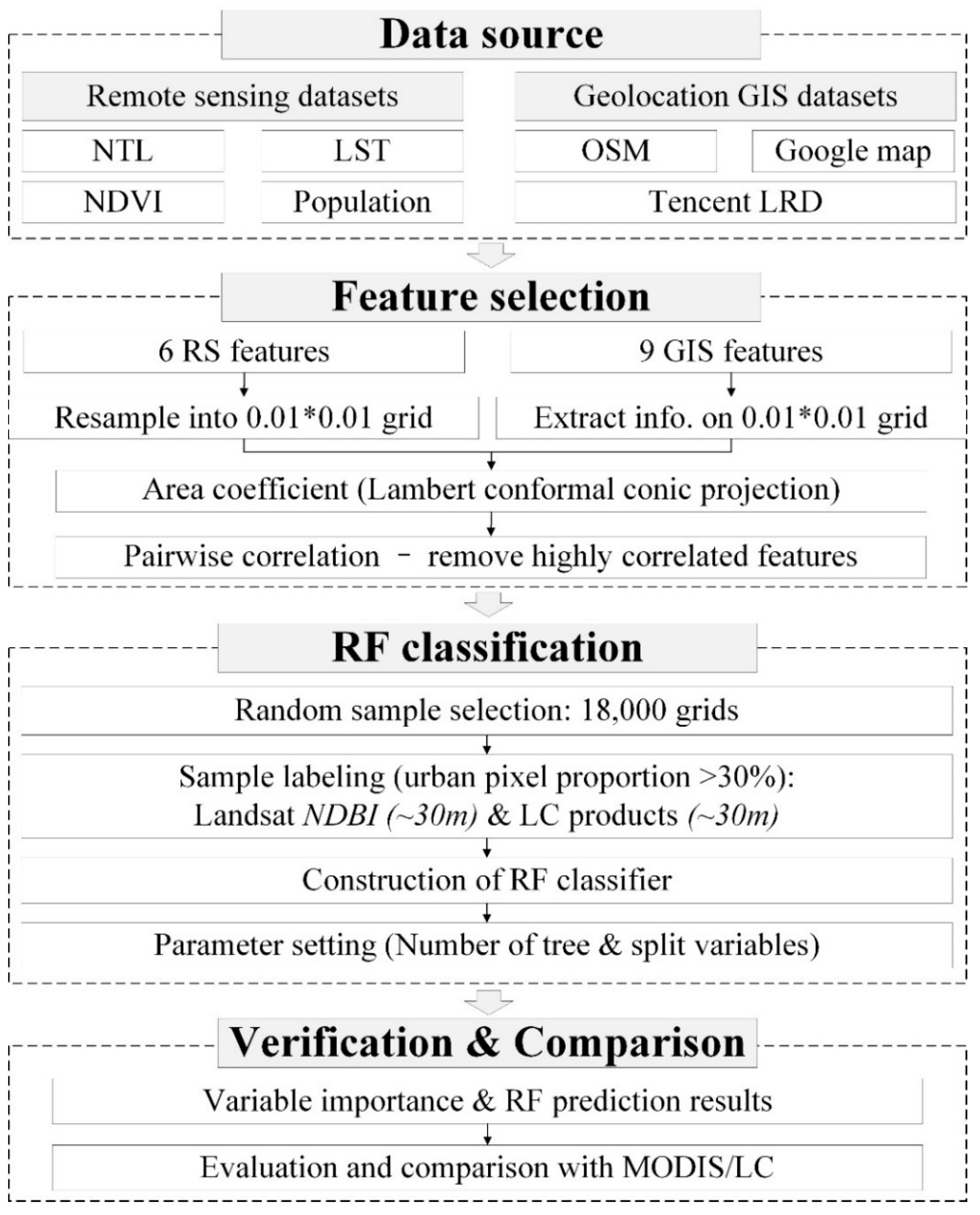
The workflow of this study is shown in Figure 2. It includes feature selection, random forest classification, and verification and comparison.
4.1. Feature Selection
4.1.1. Initial Elimination of Non-Urban Areas
To reduce noise and the computation complexity, an initial elimination process was applied to areas without a location request during the 60 monitoring days. Thus, the daily maximum LRD was composited from the original hourly Tencent data, and those pixels with an LRD equal to 0 were excluded from our study. A total of 3,680,920 pixels (0.01 × 0.01 degrees), covering about 3.71 million km2 of land area, were selected for subsequent analyses. For computation convenience, all analyses were conducted based on the 0.01 degree grid of the Tencent LRD data.
4.1.2. Tencent LRD Temporal Features
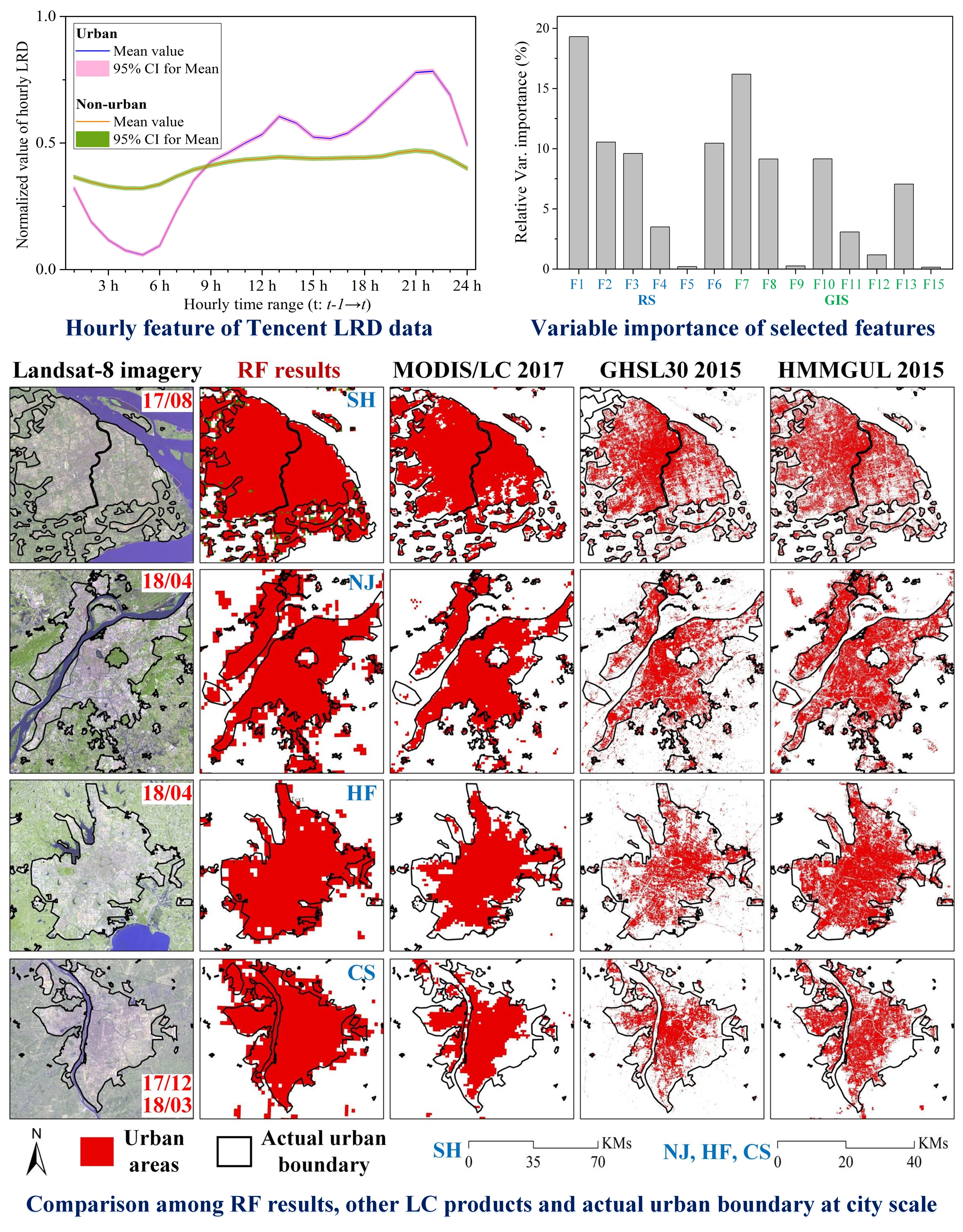
The daily average LRD is a significant and simple temporal feature, and urban areas usually gathered more location requests. The hourly temporal change pattern is also effective at distinguishing urban areas [28,37]. The hourly LRD in urban areas shows an obvious temporal change compared with that in non-urban areas based on the selected samples in Section 4.2.1 (Figure 3). These hourly features in urban areas show a similar pattern to the ones found in previous studies, including a study on Twitter data, which found a valley during 3 a.m. to 7 a.m. and an obvious increase during night-time [23]. Thus, the hourly average LRD during the 60-day research period was calculated and normalized to 0–1 to generate an hourly curve for each grid. Then, each hourly curve was compared with the reference curve shown in Figure 3. Those that were closer or more similar to the reference curve were considered to indicate a higher probability of an urban area. The average value of two indexes (Pearson’s cross-correlation coefficient and the Minkowski distance) was introduced to measure this temporal similarity [69]. The ratio of weekday average to weekend average was also added to enrich the LRD features (Table 2).
4.1.3. Feature Calculation and Selection
For a unified calculation, the 500 m RS datasets were resampled to 0.01 degree grids of the LRD dataset, and the area-weighted mean value was assigned as the new grid value (Table 2). The maximum value within each 0.01 degree grid was also calculated for those RS datasets. For the 1 km RS datasets, the original datasets were directly converted into a 0.01 degree grid using the nearest resample method in ArcMap 10.2. For the GIS datasets, all features can be directly calculated or acquired for each 0.01 degree grid. To eliminate area distortion in the WGS84 coordinate system, the coefficient of the ratio of standard area (1 km2) to actual grid area on the Lambert conformal conic projection was multiplied by the original feature value to generate a new value for all features [46].
Thus, six RS and nine GIS features were selected as potential training features, including VIIRS mean, VIIRS max, NDVI mean, NDVI max, LST, population density, LRD daily average, LRD hourly similarity, LRD weekly ratio, density of all roads, vehicle road density, nonvehicle road density, accessibility/time, accessibility/distance, and accessibility/speed (Table 2). We also determined the pairwise Spearman correlations for 15 potential features. Highly correlated (r > 0.9) variables were removed [55]. The F13 time and F14 distance features were highly correlated. F14, which was highly correlated with F15, was removed, resulting in 14 features for the RF input (Table 3).
4.2. Random Forest Classification
4.2.1. Sample Selection and Labeling
Training samples are essential for an RF classifier, and should be representative, sufficient, and high-quality [51]. In this study, the samples were classified into two categories: urban and non-urban. The average value of the urban pixel proportion from three high-resolution LC products and Landsat/NDBI was assigned to each grid, where each pixel with a >30% proportion was preliminarily labeled as an urban grid (Figure 4). The FROM-GLC30 and GHSL30 products have a similar urban pattern that differs from those of HRNTUL and NDBI to varying degrees (Figure 4). Four values were not completely consistent with the high-resolution images from the GEE. Thus, a simple manual auxiliary was used to validate the appropriateness of the calculated average value of the four proportions, and some labels that were obvious mistakes were revised. Previous studies report that the size of the training sample set should cover about 0.25% of the total study area [70]. A total of 9000 random samples were obtained for training. To increase the proportion of urban samples, one-third of all samples were chosen as urban samples.
4.2.2. Construction of the RF Classifier
The random forest classifier is an ensemble algorithm that combines a large number of decision trees and can perform better than a single classifier [50]. In an RF classifier, each decision tree is independently produced without any pruning, and can assign the most possible class to an input feature vector. The RF classifier makes tress grow from different data subsets through a bagging or bootstrap aggregating process, which increases the stability and robustness [47,71]. For an individual tree, about two-thirds of the datasets are usually included in each bagging subset for training, and the excluded samples form the out-of-bag (OOB) subset, which can be used to evaluate the performance using the OOB error [47]. Furthermore, an individual tree grows based on the best split of the randomly selected input features or predictive variables at each node. The Gini index was introduced to identify the this value and maximize the dissimilarity between designated classes using an impurity measurement [72]. The above-mentioned OOB error and the Gini index can also be used to evaluate the relative variable importance (as a percentage) of different features, where a higher relative value means a greater contribution to the prediction [43]. In this study, an RF classifier was adopted using the scikit-learn package in Python, with the related urban and non-urban probability as the result [73].
4.2.3. RF Parameter Settings
Several of the RF classifier’s parameters must be user-defined; the two most important are the number of classification trees (k) and number of split variables (m) [47]. A grid search (gs) method in Python was introduced to determine the optimal parameter values, where the model loops through predefined intervals and the parameter with the smallest OOB error is selected as the optimal value [74]. For parameter k, higher values, such as 500, will bring about a higher classification accuracy but also computation complexity problems and intercorrelations between trees [47]. Thus, we set the range of 10−500 and intervals of 10 for k as the gs method input. For parameter m, previous studies have found the optimal value to be the square root of the total number of input variables [43,75]. Thus, we set a range of 1−14 and intervals of 1 for m as the gs method input.
4.3. Verification and Comparison
Another randomly selected 9000 samples, combined with the training samples, were applied to validate the results of the urban area extraction based on the overall accuracy (OA), producer accuracy (PA), user’s accuracy (UA), and kappa coefficient. Four typical cities (Shanghai, Nanjing, Hefei, and Changsha) were selected to verify the RF prediction results at the city scale. The actual urban boundary was acquired using cadastral data from the local Land and Resource Bureau with the help of the manual interpretation of Landsat-8 images. The RF prediction results were spatially compared with high-resolution and MODIS LC products in these four cities, and numerically compared with MODIS/LC.
5. Results
5.1. Parameter Settings and Variable Importance for RF
The RF classifier has two important parameters (number of trees (k) and number of split variables (m)), and minimization of the OOB error can be used to identify their optimal values. Figure 5A shows that the OOB error converges to 10.0% and 10.02% from about 150 trees (k) with an m value of 1, 5, 10, and 14. The optimal k value was set as 150 in this study with computation complexity in mind. For parameter m, the OOB error shows a general decrease when m increases, and converges after m = 5, where the relative minimum error happens with an m value of 7 (Figure 5B). Thus, the best k value was set as 150 and the best m value was set as 7 in this study. The results on the relative variable importance of the 14 selected features show that the VIIRS and LRD features, with the highest variable importance, contribute the most to urban area prediction (Figure 6). Population density, VIIRS max, NDVI, the LRD hourly feature, and accessibility—time show a moderate influence on the RF classifier’s performance. Moreover, LST, accessibility—speed, and the LRD weekly ratio have almost no influence on the RF prediction results.
5.2. Urban Extraction Results
The RF classifier made a prediction on the class (urban or non-urban) of each pixel and provided a probability for each class. Only pixels with a high probability were classified as urban areas. In summary, 172,170 pixels were classified as urban areas, with a probability that was greater than 0.5, covering an area of 176,266 km2 under Lambert conformal conic projection. Figure 7 shows that the urban pixels with a high probability are mainly concentrated in the eastern and southeast coastal regions of China. There is a sparser distribution of urban areas in the northeast and west regions. This distribution pattern is consistent with the level of urban development in China. We can also observe that pixels with a high probability aggregate in the center of the urban areas. According to the statistics, there is a slight decrease when the urban probability increases from 0.5 to 0.85 and a sharp increase after 0.85 (Figure 8). This also indicates the aggregation of urban areas, and stronger correlations among input features for regions closer to a city’s center (Figure 9).
The three most developed regions (the Yangtze River Delta, Beijing–Tianjin–Hebei, and the Pearl River Delta) were selected to display in detail (Figure 7). The regional center city is well-identified by the RF classifier, and the urban outlines are well-demarcated. We also compared the spatial pattern of different features with the RF results at the city level (Figure 9). Due to the large variable importance, the RF classifier results show the most similar spatial pattern to those of the VIIRS and LRD features, which have a higher level of differentiation between urban and non-urban areas. The higher contribution of VIIRS and LRD also proves that socioeconomic factors contribute the most to the distribution of urban areas [41]. The RF classifier can also avoid some defects of other datasets, such as the NDVI dataset’s underestimation of urban fringe areas, and the OSM and VIIRS datasets’ overestimation of external road areas.
5.3. Accuracy and Comparison
The OA based on the training dataset and the validation dataset is 91.80% and 89.79%, respectively, where the training samples show a better performance than the validation samples (Table 4). The PA, UA, and OA for non-urban extraction are slightly higher than those for urban area extraction for both the training and validation samples. The OA for all samples is 90.79%, with a kappa value of 0.790, indicating a good classification result. Moreover, the absence of NTL or LRD features (with only 13 features as input) causes the largest decrease in OA (approximately 20%, Figure 6). This is also consistent with the variable importance rankings, and proves the usefulness of the geolocation dataset.
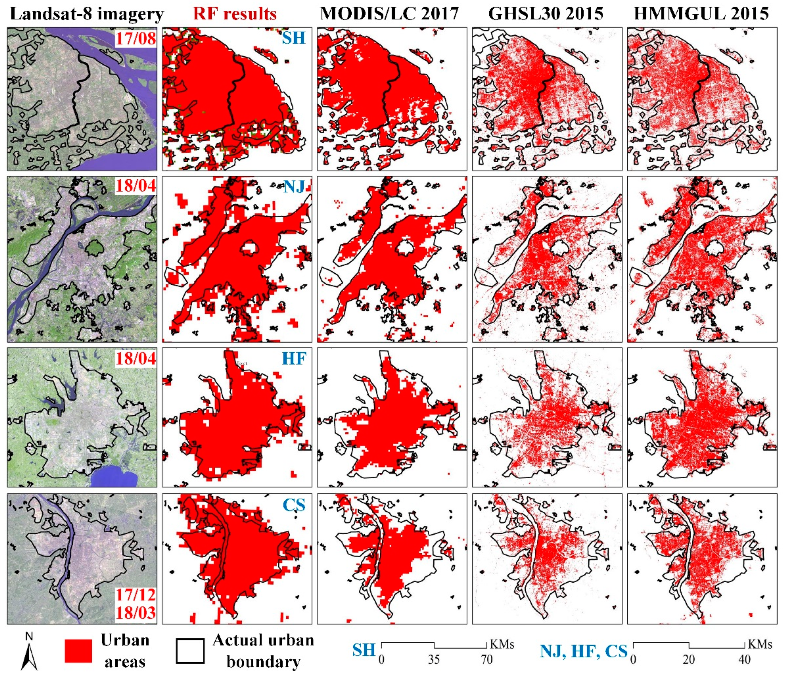
We also compared the RF classifier results with the actual urban boundary for the four selected cities (Figure 10). Our classification results are in good accordance with the urban boundaries, and small urban areas around the core city are also identified by our model.
However, due to the coarse resolution, our model shows an obvious misclassification in river and lake regions, especially for Changsha and Shanghai. For the high-resolution LC products, some non-urban areas with non-construction LC types can be detected that are still recognized as urban areas by the government (Figure 10). These areas commonly have a high number of VIIRS and LRD features, just like urban areas with construction LC. Compared with the MODIS/LC product, the RF classification results with respect to both total area and spatial pattern are closer to the manual interpretation results, whereas MODIS/LC tends to greatly underestimate the urban areas (Table 5). The RF classifier can predict small urban areas more accurately. However, our RF classifier still shows overestimation in some fringe areas and small urban areas around the core cities.
6. Discussions
6.1. Feature Selection for Urban Extraction
Different feature selections or combinations will greatly affect the RF classification results, and our selected features have covered the main driving forces for urban expansion, including socioeconomic, physical, proximity, and neighborhood factors [41]. Some of these features are well-correlated, such as F10 (all road), F11 (vehicle road), and F12 (nonvehicle road), which were calculated from the same road network dataset, with F10 the summation of F11 and F12 for each grid (Table 3). However, their contributions to the RF prediction result are different; F10’s contribution is twice F11’s contribution and four times F12’s contribution (Figure 6). The exclusion of features with a small variable importance, such as F5, F9, and F15, may also result in a slight drop in overall accuracy (Figure 6). This means that we cannot exclude or merge any features based only on their contribution, and that only highly correlated (r > 0.9) features can be excluded [55]. Thus, a larger number of input features, including those with a lower contribution to the classification, tend to result in higher classification performance [32]. In a future study, more open-access geolocation data could be applied, such as point-of-interest (POI) data, from both field measurements and crowd sourcing [28,76].
We also applied the RF classifier using only RS features. An approximately 80% overestimation of total areas was obtained, which proves that it is necessary to combine RS feature datasets with geolocation GIS datasets. In moderate-resolution RS datasets, urban and rural areas sometimes have similar features, and these datasets may lack accurate human activity and socioeconomic information [77,78]. For example, some small industrial parks areas may have similar optical characteristics to non-urban areas, and LC products cannot be fully identified from diurnal images only (Figure 11A). The features of LRD, supporting roads, and NTL can help to identify these areas with high-level values. For a fallow period in some farmland areas, bare lands can be misclassified as urban areas when only using optical images from existing LC products (Figure 11B). These areas can be correctly labeled using supplementary information on low-level NTL, LRD, and road density.
6.2. Samples and Parameters for the RF Classifier
The RF classifier combines several individual decision trees, and can handle high dimensional and multiple collinear features, resulting in insensitivity to overfitting [51]. Sample selection and labeling are the key problems for prediction. In our study, samples were created using simple sampling methods, and only the average value of four types of urban pixel proportion was set as the labeling reference. This process is efficient and can save a lot of time compared with direct manual interpretation of high-resolution imagery for each sample. However, there are obvious differences among four types of urban pixel proportion (Figure 4), and other statistics may improve the reliability of the urban proportion. However, both the average value and other statistical features would bring about systematic error, and error correction by manual validation would inevitably need to be performed to improve the sample’s accuracy [79]. Thus, simple average statistics for the urban pixel proportion were applied instead of other statistics.
We also conducted a statistical analysis of the urban samples. The heatmap analysis results show that most of the urban samples had a low urban proportion, while the two most important variables (F1 and F7) have no obvious correlation with the urban proportion (Figure 12A). Most of the urban samples were found to have a low-level urban pixel proportion, which is consistent with a situation in which most of the urban areas contain a certain number of non-construction LC types. This also proves the randomness of the sample selection and labeling’s reliability. The urban probability determined by the RF classifier shows a concentrated Log curve distribution with two variables, and is strongly influenced by these two variables, which is consistent with the variable importance results (Figure 6 and Figure 12B).
Another important aspect of RF classifiers is the setting of key parameters. Overall, the OOB error was found to tend to converge as the values of the two parameters increase. According to previous studies, k is less sensitive to classification accuracy than m. Thus, the inflection point of the k convergence curve was selected to balance accuracy and calculation. For the more sensitive m parameter, the value with the minimum OOB error was selected to minimize the influence on the prediction results. There is another important parameter in RF prediction results: the probability threshold, which can also greatly influence the total number of extraction results. From the city-scale display in Figure 10, we can observe slightly larger urban areas compared with the actual urban boundaries. If the probability threshold were set to 0.6, the prediction results would be closer to the actual scale and pattern. This means that the constraint condition of the total amount of other information can guide the selection of an appropriate probability (instead of 0.5 as a threshold) and deserves further study.
6.3. Data Reliability and Comparison with Other Machine Learning (ML) Methods
The geolocation GIS datasets used in this study are all web-sourced, including the Tencent LRD, OSM, and Google Map API datasets, with a low acquisition cost. Although these datasets are widely used in other studies, the reliability of these open-access datasets has not been systematically evaluated, and they are not absolutely reliable. In contrast to the objectivity of the RS dataset, the geolocation dataset is somewhat subjective, partial, and not authoritative [77]. The Tencent LRD data are not absolutely reliable and comprehensive, even though they have already proven to be successful in mapping land use/cover [33,80]. For example, not everyone in China uses Tencent’s location service, and normal users cannot use it all the time. Thus, the Tencent LRD data can only reflect a relative value, not an absolute value. Moreover, we also observed some noise outside the clear boundaries due to travel and geolocation deviations (Figure 9). However, most of the previous studies used parcel-, community-, or city-scale geolocation datasets. The LRD dataset remains the optimal dataset for large-scale urban mapping [19,29,44].
We also used the SVM and ANN (Keras) classifiers just for the selected samples. The prediction results showed that the OA of the SVM classifier was lower than that of the RF classifier by about 7%, but had a lower training and classification time. For the ANN classifier, the OA was slightly higher than that of the RF classifier by about 2%, but the training time was greatly increased. We did not optimize the parameters for the SVM and ANN classifiers; however, the RF classifier remains the optimal classifier for combinations of RS and geolocation datasets. Even so, our model and results were greatly limited by the low-spatial-resolution and outdated datasets, which increased the uncertainty in urban fringe areas. Geolocation data with a finer resolution should be preferentially evaluated to match with mature medium- or high-resolution RS datasets, such as Landsat-8 or Sentinel-2, to provide a finer spatial resolution urban area product.
7. Conclusion
In this study, we integrated multi-source RS and geolocation GIS datasets to extract urban areas in China. Tencent location requests density (LRD) data were used to record the large-scale human activity intensity, and temporal features were used to distinguish urban areas. The random forest (RF) classifier was applied to extract urban areas based on six RS and eight GIS features at the spatial resolution of 0.01 degree. The results showed that night-time light and LRD features had the largest variable importance, which proved the usefulness of geolocation datasets. A total of 176,266 km2 of urban areas in China were identified using the RF classifier, with an overall accuracy of 90.79% and a kappa coefficient of 0.790. Our results were highly consistent with the boundaries that we obtained by manual interpretation in four selected cities.
However, there are still improvements to be made. The reliability of web-sourced GIS data should be evaluated systematically. More RS and geolocation GIS data could be applied to extract urban areas at a large scale, especially geolocation datasets with a finer spatial resolution. For sample selection and labeling, more reliable information could be introduced to improve the samples, which may reduce the amount of required manual validation work. In future work, a comparison between different machine learning methods can be performed for combinations of RS and geolocation datasets and different combinations of various features. Moreover, the urban structure and other important urban characteristics could also be identified.
Author Contributions
Conceptualization, L.C. and M.L.; Methodology, L.C. and M.L.; Validation, N.X.; Formal analysis, N.X.; Resources, M.L. and N.X.; Writing—original draft preparation, N.X. and L.C.; Writing—review and editing, M.L. and N.X.; Visualization, N.X.; Project administration, N.X. and L.C.; Funding acquisition, L.C. and M.L.
Funding
This research was supported by the National Key Research and Development Plan (2017YFB0504205) and the National Science Foundation of China (41622109, 41371017).
Acknowledgments
Sincere thanks are given to the anonymous reviewers and members of the editorial team for their comments and contributions.
Conflicts of Interest
The authors declare no conflict of interest.
References
- Foley, J.A.; DeFries, R.; Asner, G.P.; Barford, C.; Bonan, G.; Carpenter, S.R.; Chapin, F.S.; Coe, M.T.; Daily, G.C.; Gibbs, H.K.; et al. Global consequences of land use. Science 2005, 309, 570–574. [Google Scholar] [CrossRef]
- Schneider, A.; Friedl, M.A.; Potere, D. A new map of global urban extent from MODIS satellite data. Environ. Res. Lett. 2009, 4. [Google Scholar] [CrossRef]
- Xie, Y.H.; Weng, Q.H. Updating urban extents with nighttime light imagery by using an object-based thresholding method. Remote Sens. Environ. 2016, 187, 1–13. [Google Scholar] [CrossRef]
- Zhou, D.C.; Zhao, S.Q.; Zhang, L.X.; Liu, S.G. Remotely sensed assessment of urbanization effects on vegetation phenology in China’s 32 major cities. Remote Sens. Environ. 2016, 176, 272–281. [Google Scholar] [CrossRef]
- National Bureau of Statistics of China. Annual Statistical Yearbook of China. Available online: http://www.stats.gov.cn/english/Statisticaldata/AnnualData/ (accessed on 8 January 2019).
- Deng, X.Z.; Huang, J.K.; Rozelle, S.; Zhang, J.P.; Li, Z.H. Impact of urbanization on cultivated land changes in China. Land Use Policy 2015, 45, 1–7. [Google Scholar] [CrossRef]
- Kuang, W.H.; Liu, J.Y.; Dong, J.W.; Chi, W.F.; Zhang, C. The rapid and massive urban and industrial land expansions in China between 1990 and 2010: A CLUD-based analysis of their trajectories, patterns, and drivers. Landsc. Urban Plan. 2016, 145, 21–33. [Google Scholar] [CrossRef]
- Wei, Y.H.D.; Li, H.; Yue, W.Z. Urban land expansion and regional inequality in transitional China. Landsc. Urban Plan. 2017, 163, 17–31. [Google Scholar] [CrossRef]
- Ma, T.; Zhou, C.H.; Pei, T.; Haynie, S.; Fan, J.F. Quantitative estimation of urbanization dynamics using time series of DMSP/OLS nighttime light data: A comparative case study from China’s cities. Remote Sens. Environ. 2012, 124, 99–107. [Google Scholar] [CrossRef]
- Liu, X.; de Sherbinin, A.; Zhan, Y. Mapping Urban Extent at Large Spatial Scales Using Machine Learning Methods with VIIRS Nighttime Light and MODIS Daytime NDVI Data. Remote Sens. 2019, 11, 1247. [Google Scholar] [CrossRef]
- Zhou, Y.Y.; Smith, S.J.; Elvidge, C.D.; Zhao, K.G.; Thomson, A.; Imhoff, M. A cluster-based method to map urban area from DMSP/OLS nightlights. Remote Sens. Environ. 2014, 147, 173–185. [Google Scholar] [CrossRef]
- Jing, W.L.; Yang, Y.P.; Yue, X.F.; Zhao, X.D. Mapping Urban Areas with Integration of DMSP/OLS Nighttime Light and MODIS Data Using Machine Learning Techniques. Remote Sens. 2015, 7, 12419–12439. [Google Scholar] [CrossRef] [Green Version]
- Goldblatt, R.; Stuhlmacher, M.F.; Tellman, B.; Clinton, N.; Hanson, G.; Georgescu, M.; Wang, C.Y.; Serrano-Candela, F.; Khandelwal, A.K.; Cheng, W.H.; et al. Using Landsat and nighttime lights for supervised pixel-based image classification of urban land cover. Remote Sens. Environ. 2018, 205, 253–275. [Google Scholar] [CrossRef]
- Zhang, Q.L.; Schaaf, C.; Seto, K.C. The Vegetation Adjusted NTL Urban Index: A new approach to reduce saturation and increase variation in nighttime luminosity. Remote Sens. Environ. 2013, 129, 32–41. [Google Scholar] [CrossRef]
- Zhang, X.Y.; Li, P.J. A temperature and vegetation adjusted NTL urban index for urban area mapping and analysis. ISPRS J. Photogramm. Remote Sens. 2018, 135, 93–111. [Google Scholar] [CrossRef]
- Zhang, X.Y.; Li, P.J.; Cai, C. Regional Urban Extent Extraction Using Multi-Sensor Data and One-Class Classification. Remote. Sens. 2015, 7, 7671–7694. [Google Scholar] [CrossRef] [Green Version]
- Huang, X.M.; Schneider, A.; Friedl, M.A. Mapping sub-pixel urban expansion in China using MODIS and DMSP/OLS nighttime lights. Remote Sens. Environ. 2016, 175, 92–108. [Google Scholar] [CrossRef]
- Liu, Y.; Liu, X.; Gao, S.; Gong, L.; Kang, C.G.; Zhi, Y.; Chi, G.H.; Shi, L. Social Sensing: A New Approach to Understanding Our Socioeconomic Environments. Ann. Assoc. Am. Geogr. 2015, 105, 512–530. [Google Scholar] [CrossRef]
- Hu, T.Y.; Yang, J.; Li, X.C.; Gong, P. Mapping Urban Land Use by Using Landsat Images and Open Social Data. Remote Sens. 2016, 8. [Google Scholar] [CrossRef]
- Shelton, T.; Poorthuis, A.; Zook, M. Social media and the city: Rethinking urban socio-spatial inequality using user-generated geographic information. Landsc. Urban Plan. 2015, 142, 198–211. [Google Scholar] [CrossRef]
- Fu, C.; McKenzie, G.; Frias-Martinez, V.; Stewart, K. Identifying spatiotemporal urban activities through linguistic signatures. Comput. Environ. Urban Syst. 2018, 72, 25–37. [Google Scholar] [CrossRef]
- Zhen, F.; Cao, Y.; Qin, X.; Wang, B. Delineation of an urban agglomeration boundary based on Sina Weibo microblog ‘check-in’ data: A case study of the Yangtze River Delta. Cities 2017, 60, 180–191. [Google Scholar] [CrossRef]
- Garcia-Palomares, J.C.; Salas-Olmedo, M.H.; Moya-Gomez, B.; Condeco-Melhorado, A.; Gutierrez, J. City dynamics through Twitter: Relationships between land use and spatiotemporal demographics. Cities 2018, 72, 310–319. [Google Scholar] [CrossRef]
- Du, S.H.; Zhang, F.L.; Zhang, X.Y. Semantic classification of urban buildings combining VHR image and GIS data: An improved random forest approach. ISPRS J. Photogramm. Remote Sens. 2015, 105, 107–119. [Google Scholar] [CrossRef]
- Zhang, X.Y.; Du, S.H.; Wang, Q. Hierarchical semantic cognition for urban functional zones with VHR satellite images and POI data. ISPRS J. Photogramm. Remote Sens. 2017, 132, 170–184. [Google Scholar] [CrossRef]
- Guo, Z.; Du, S. Mining parameter information for building extraction and change detection with very high-resolution imagery and GIS data. GISci. Remote Sens. 2017, 54, 38–63. [Google Scholar] [CrossRef]
- Deng, C.B.; Wu, C.S. The use of single-date MODIS imagery for estimating large-scale urban impervious surface fraction with spectral mixture analysis and machine learning techniques. ISPRS J. Photogramm. Remote Sens. 2013, 86, 100–110. [Google Scholar] [CrossRef]
- Chen, Y.H.; Ge, Y.; An, R.; Chen, Y. Super-Resolution Mapping of Impervious Surfaces from Remotely Sensed Imagery with Points-of-Interest. Remote Sens. 2018, 10. [Google Scholar] [CrossRef]
- Tu, W.; Hu, Z.W.; Li, L.F.; Cao, J.Z.; Jiang, J.C.; Li, Q.P.; Li, Q.Q. Portraying Urban Functional Zones by Coupling Remote Sensing Imagery and Human Sensing Data. Remote Sens. 2018, 10. [Google Scholar] [CrossRef]
- Bennett, M.M.; Smith, L.C. Advances in using multitemporal night-time lights satellite imagery to detect, estimate, and monitor socioeconomic dynamics. Remote Sens. Environ. 2017, 192, 176–197. [Google Scholar] [CrossRef]
- Levin, N. The impact of seasonal changes on observed nighttime brightness from 2014 to 2015 monthly VIIRS DNB composites. Remote Sens. Environ. 2017, 193, 150–164. [Google Scholar] [CrossRef]
- Cai, J.X.; Huang, B.; Song, Y.M. Using multi-source geospatial big data to identify the structure of polycentric cities. Remote Sens. Environ. 2017, 202, 210–221. [Google Scholar] [CrossRef]
- Zhang, Y.; Li, Q.Z.; Huang, H.P.; Wu, W.; Du, X.; Wang, H.Y. The Combined Use of Remote Sensing and Social Sensing Data in Fine-Grained Urban Land Use Mapping: A Case Study in Beijing, China. Remote Sens. 2017, 9. [Google Scholar]
- Ladle, A.; Galpern, P.; Doyle-Baker, P. Measuring the use of green space with urban resource selection functions: An application using smartphone GPS locations. Landsc. Urban Plan. 2018, 179, 107–115. [Google Scholar] [CrossRef]
- Ma, T. Multi-Level Relationships between Satellite-Derived Nighttime Lighting Signals and Social Media-Derived Human Population Dynamics. Remote Sens. 2018, 10. [Google Scholar] [CrossRef]
- Niu, N.; Liu, X.P.; Jin, H.; Ye, X.Y.; Liu, Y.; Li, X.; Chen, Y.M.; Li, S.Y. Integrating multi-source big data to infer building functions. Int. J. Geogr. Inf. Sci. 2017, 31, 1871–1890. [Google Scholar] [CrossRef]
- Chen, Y.M.; Liu, X.P.; Li, X.; Liu, X.J.; Yao, Y.; Hu, G.H.; Xu, X.C.; Pei, F.S. Delineating urban functional areas with building-level social media data: A dynamic time warping (DTW) distance based k-medoids method. Landsc. Urban Plan. 2017, 160, 48–60. [Google Scholar] [CrossRef]
- Xu, J.; Li, A.Y.; Li, D.; Liu, Y.; Du, Y.Y.; Pei, T.; Ma, T.; Zhou, C.H. Difference of urban development in China from the perspective of passenger transport around Spring Festival. Appl. Geogr. 2017, 87, 85–96. [Google Scholar] [CrossRef]
- Xing, H.F.; Meng, Y. Integrating landscape metrics and socioeconomic features for urban functional region classification. Comput. Environ. Urban 2018, 72, 134–145. [Google Scholar] [CrossRef]
- Wei, Y.; Song, W.; Xiu, C.L.; Zhao, Z.Y. The rich-club phenomenon of China’s population flow network during the country’s spring festival. Appl. Geogr. 2018, 96, 77–85. [Google Scholar] [CrossRef]
- Li, G.D.; Sun, S.A.; Fang, C.L. The varying driving forces of urban expansion in China: Insights from a spatial-temporal analysis. Landsc. Urban Plan. 2018, 174, 63–77. [Google Scholar] [CrossRef]
- Weiss, D.J.; Nelson, A.; Gibson, H.S.; Temperley, W.; Peedell, S.; Lieber, A.; Hancher, M.; Poyart, E.; Belchior, S.; Fullman, N.; et al. A global map of travel time to cities to assess inequalities in accessibility in 2015. Nature 2018, 553, 333. [Google Scholar] [CrossRef] [PubMed]
- Gislason, P.O.; Benediktsson, J.A.; Sveinsson, J.R. Random Forests for land cover classification. Pattern Recogn. Lett. 2006, 27, 294–300. [Google Scholar] [CrossRef]
- Liu, Y.; Delahunty, T.; Zhao, N.Z.; Cao, G.F. These lit areas are undeveloped: Delimiting China’s urban extents from thresholded nighttime light imagery. Int. J. Appl. Earth Obs. 2016, 50, 39–50. [Google Scholar] [CrossRef]
- Zhang, P.Y.; Pan, J.J.; Xie, L.T.; Zhou, T.; Bai, H.R.; Zhu, Y.X. Spatial-Temporal Evolution and Regional Differentiation Features of Urbanization in China from 2003 to 2013. ISPRS Int. J. Geo-Inf. 2019, 8. [Google Scholar] [CrossRef]
- Cao, X.; Chen, J.; Imura, H.; Higashi, O. A SVM-based method to extract urban areas from DMSP-OLS and SPOT VGT data. Remote Sens. Environ. 2009, 113, 2205–2209. [Google Scholar] [CrossRef]
- Rodriguez-Galiano, V.F.; Ghimire, B.; Rogan, J.; Chica-Olmo, M.; Rigol-Sanchez, J.P. An assessment of the effectiveness of a random forest classifier for land-cover classification. ISPRS J. Photogramm. Remote Sens. 2012, 67, 93–104. [Google Scholar] [CrossRef]
- Xu, T.T.; Coco, G.; Gao, J. Extraction of urban built-up areas from nighttime lights using artificial neural network. Geocarto Int. 2019. [Google Scholar] [CrossRef]
- Chen, Z.Q.; Yu, B.L.; Zhou, Y.Y.; Liu, H.X.; Yang, C.S.; Shi, K.F.; Wu, J.P. Mapping Global Urban Areas From 2000 to 2012 Using Time-Series Nighttime Light Data and MODIS Products. IEEE J. Sel. Top. Appl. Earth Obs. Remote Sens. 2019, 12, 1143–1153. [Google Scholar] [CrossRef]
- Breiman, L. Random forests. Mach. Learn. 2001, 45, 5–32. [Google Scholar] [CrossRef]
- Belgiu, M.; Dragut, L. Random forest in remote sensing: A review of applications and future directions. ISPRS J. Photogramm. Remote Sens. 2016, 114, 24–31. [Google Scholar] [CrossRef]
- Pham, L.T.H.; Brabyn, L.; Ashraf, S. Combining QuickBird, LiDAR, and GIS topography indices to identify a single native tree species in a complex landscape using an object-based classification approach. Int. J. Appl. Earth Obs. 2016, 50, 187–197. [Google Scholar] [CrossRef]
- Mellor, A.; Boukir, S. Exploring diversity in ensemble classification: Applications in large area land cover mapping. ISPRS J. Photogramm. Remote Sens. 2017, 129, 151–161. [Google Scholar] [CrossRef]
- Rasanen, A.; Kuitunen, M.; Tomppo, E.; Lensu, A. Coupling high-resolution satellite imagery with ALS-based canopy height model and digital elevation model in object-based boreal forest habitat type classification. ISPRS J. Photogramm. Remote Sens. 2014, 94, 169–182. [Google Scholar] [CrossRef] [Green Version]
- Millard, K.; Richardson, M. On the Importance of Training Data Sample Selection in Random Forest Image Classification: A Case Study in Peatland Ecosystem Mapping. Remote Sens. 2015, 7, 8489–8515. [Google Scholar] [CrossRef] [Green Version]
- Jin, H.R.; Stehman, S.V.; Mountrakis, G. Assessing the impact of training sample selection on accuracy of an urban classification: A case study in Denver, Colorado. Int. J. Remote Sens. 2014, 35, 2067–2081. [Google Scholar] [CrossRef]
- Sulla-Menashe, D.; Friedl, M.A. User Guide to Collection 6 MODIS Land Cover (MCD12Q1 and MCD12C1) Product; USGS: Reston, VA, USA, 2018. Available online: https://lpdaac.usgs.gov/sites/default/files/public/product_documentation/mcd12_user_guide_v6.pdf (accessed on 1 December 2018).
- Gong, P.; Wang, J.; Yu, L.; Zhao, Y.C.; Zhao, Y.Y.; Liang, L.; Niu, Z.G.; Huang, X.M.; Fu, H.H.; Liu, S.; et al. Finer resolution observation and monitoring of global land cover: First mapping results with Landsat TM and ETM+ data. Int. J. Remote Sens. 2013, 34, 2607–2654. [Google Scholar] [CrossRef]
- Pesaresi, M.; Guo, H.D.; Blaes, X.; Ehrlich, D.; Ferri, S.; Gueguen, L.; Halkia, M.; Kauffmann, M.; Kemper, T.; Lu, L.L.; et al. A Global Human Settlement Layer From Optical HR/VHR RS Data: Concept and First Results. IEEE J. Sel. Top. Appl. Earth Obs. Remote Sens. 2013, 6, 2102–2131. [Google Scholar] [CrossRef]
- Liu, X.P.; Hu, G.H.; Chen, Y.M.; Li, X.; Xu, X.C.; Li, S.Y.; Pei, F.S.; Wang, S.J. High-resolution multi-temporal mapping of global urban land using Landsat images based on the Google Earth Engine Platform. Remote Sens. Environ. 2018, 209, 227–239. [Google Scholar] [CrossRef]
- National Centers for Environment Information (NCEI). National Oceanic and Atmospheric Administration (NOAA). Available online: http://www.ngdc.noaa.gov/eog/viirs/ download_monthly.html (accessed on 1 March 2019).
- Lu, D.S.; Tian, H.Q.; Zhou, G.M.; Ge, H.L. Regional mapping of human settlements in southeastern China with multisensor remotely sensed data. Remote Sens. Environ. 2008, 112, 3668–3679. [Google Scholar] [CrossRef]
- Peng, S.S.; Piao, S.L.; Ciais, P.; Friedlingstein, P.; Ottle, C.; Breon, F.M.; Nan, H.J.; Zhou, L.M.; Myneni, R.B. Surface Urban Heat Island Across 419 Global Big Cities. Environ. Sci. Technol. 2012, 46, 696–703. [Google Scholar] [CrossRef]
- CIESIN—Center for International Earth Science Information Network—Columbia University. Gridded Population of the World, Version 4 (GPWv4): Population Density; NASA Socioeconomic Data and Applications Center (SEDAC): Palisades, NY, USA, 2016. Available online: http://dx.doi.org/10.7927/H4NP22DQ (accessed on 20 March 2019).
- Tecent Location Big Data. Available online: https://heat.qq.com/ (accessed on 10 May 2019). (In Chinese).
- Li, Y.; He, P.; Hu, Y.; Chen, C.; Jing, N. System and Method for Processing Location Data of Target User. U.S. Patent Application No. 14/699,073, 26 April 2015. [Google Scholar]
- Liu, X.P.; He, J.L.; Yao, Y.; Zhang, J.B.; Liang, H.L.; Wang, H.; Hong, Y. Classifying urban land use by integrating remote sensing and social media data. Int. J. Geogr. Inf. Sci. 2017, 31, 1675–1696. [Google Scholar] [CrossRef]
- Zha, Y.; Gao, J.; Ni, S. Use of normalized difference built-up index in automatically mapping urban areas from TM imagery. Int. J. Remote Sens. 2003, 24, 583–594. [Google Scholar] [CrossRef]
- Lhermitte, S.; Verbesselt, J.; Verstraeten, W.W.; Coppin, P. A comparison of time series similarity measures for classification and change detection of ecosystem dynamics. Remote Sens. Environ. 2011, 115, 3129–3152. [Google Scholar] [CrossRef]
- Colditz, R.R. An Evaluation of Different Training Sample Allocation Schemes for Discrete and Continuous Land Cover Classification Using Decision Tree-Based Algorithms. Remote Sens. 2015, 7, 9655–9681. [Google Scholar] [CrossRef] [Green Version]
- Verikas, A.; Gelzinis, A.; Bacauskiene, M. Mining data with random forests: A survey and results of new tests. Pattern Recogn. 2011, 44, 330–349. [Google Scholar] [CrossRef]
- Pal, M.; Mather, P.M. An assessment of the effectiveness of decision tree methods for land cover classification. Remote Sens. Environ. 2003, 86, 554–565. [Google Scholar] [CrossRef]
- Pedregosa, F.; Varoquaux, G.; Gramfort, A.; Michel, V.; Thirion, B.; Grisel, O.; Blondel, M.; Prettenhofer, P.; Weiss, R.; Dubourg, V.; et al. Scikit-learn: Machine Learning in Python. J. Mach. Learn. Res. 2011, 12, 2825–2830. [Google Scholar]
- Georganos, S.; Grippa, T.; Vanhuysse, S.; Lennert, M.; Shimoni, M.; Kalogirou, S.; Wolff, E. Less is more: Optimizing classification performance through feature selection in a very-high-resolution remote sensing object-based urban application. GISci. Remote Sens. 2018, 55, 221–242. [Google Scholar] [CrossRef]
- Ghosh, A.; Fassnacht, F.E.; Joshi, P.K.; Koch, B. A framework for mapping tree species combining hyperspectral and LiDAR data: Role of selected classifiers and sensor across three spatial scales. Int. J. Appl. Earth Obs. 2014, 26, 49–63. [Google Scholar] [CrossRef]
- Li, J.; Long, Y.; Dang, A.R. Live-Work-Play Centers of Chinese cities: Identification and temporal evolution with emerging data. Comput. Environ. Urban Syst. 2018, 71, 58–66. [Google Scholar] [CrossRef]
- Zhao, N.; Cao, G.; Zhang, W.; Samson, E.L. Tweets or nighttime lights: Comparison for preeminence in estimating socioeconomic factors. ISPRS J. Photogramm. Remote Sens. 2018, 146, 1–10. [Google Scholar] [CrossRef]
- Lu, H.M.; Zhang, M.L.; Sun, W.W.; Li, W.Y. Expansion Analysis of Yangtze River Delta Urban Agglomeration Using DMSP/OLS Nighttime Light Imagery for 1993 to 2012. Isprs Int. J. Geo-Inf. 2018, 7. [Google Scholar] [CrossRef]
- Broich, M.; Stehman, S.V.; Hansen, M.C.; Potapov, P.; Shimabukuro, Y.E. A comparison of sampling designs for estimating deforestation from Landsat imagery: A case study of the Brazilian Legal Amazon. Remote Sens. Environ. 2009, 113, 2448–2454. [Google Scholar] [CrossRef]
- Levin, N.; Ali, S.; Crandall, D. Utilizing remote sensing and big data to quantify conflict intensity: The Arab Spring as a case study. Appl. Geogr. 2018, 94, 1–17. [Google Scholar] [CrossRef]
Figure 1.
The basic situation of China, including (A) the Moderate Resolution Imaging Spectroradiometer (MODIS) land cover (LC) in 2017, (B) the Visible Infrared Imaging radiometer Suite—Day/Night Band (VIIRS/DNB) intensity in October 2018, (C) the population density in 2015, and (D) the Tencent location request density (LRD) during September to November in 2018.

Figure 2.
The workflow of urban area extraction based on the random forest (RF) classifier.

Figure 3.
The normalized value of hourly LRD for urban and non-urban samples during the research period.
Figure 3.
The normalized value of hourly LRD for urban and non-urban samples during the research period.

Figure 4.
Four samples (0.01*0.01 degrees) of urban areas from 2015 FROM-GLC30, 2015 GHSL30, and 2015 HMMGUL, the 2017 Landsat Normalized Difference Built-Up Index (NDBI), and high-resolution imagery from 2017 from the Google Earth Engine (GEE) platform. The number in the four columns on the left shows the proportion of urban pixels. The text in the last column describes the average proportion and the final label.

Figure 5.
The settings for the RF classifier parameters number of trees (A) and number of split variables (B) based on the out-of-bag (OOB) error.
Figure 5.
The settings for the RF classifier parameters number of trees (A) and number of split variables (B) based on the out-of-bag (OOB) error.

Figure 6.
The relative variable importance (sum up to 100%) of the six RS features and the eight GIS features in urban extraction based on the OOB error. The overall accuracy (OA) of the absence of a related feature with 13 features as the training input. The feature codes can be found in Table 2.
Figure 6.
The relative variable importance (sum up to 100%) of the six RS features and the eight GIS features in urban extraction based on the OOB error. The overall accuracy (OA) of the absence of a related feature with 13 features as the training input. The feature codes can be found in Table 2.

Figure 7.
The probability (Prob.) of urban area extraction using the random forest classifier. (A, B, and C) show the result for the Yangtze River Delta (YRD), Beijing–Tianjin–Hebei (BTH), and Pearl River Delta (PRD) regions, respectively.
Figure 7.
The probability (Prob.) of urban area extraction using the random forest classifier. (A, B, and C) show the result for the Yangtze River Delta (YRD), Beijing–Tianjin–Hebei (BTH), and Pearl River Delta (PRD) regions, respectively.

Figure 8.
The frequency count and cumulative frequency for urban probability (≥0.5) for the RF classifier.
Figure 8.
The frequency count and cumulative frequency for urban probability (≥0.5) for the RF classifier.

Figure 9.
The city-level VIIRS, NDVI, hourly LRD similarity (H. LRD Sim.), road density, and RF probability (Prob.) result for Shanghai, Changsha, Chengdu, and Wuhan, respectively.
Figure 9.
The city-level VIIRS, NDVI, hourly LRD similarity (H. LRD Sim.), road density, and RF probability (Prob.) result for Shanghai, Changsha, Chengdu, and Wuhan, respectively.

Figure 10.
A comparison of the Landsat 8 imagery (SWIR2-SWIR1-Red), MODIS/LC 2017, GHSL30 2015, HMMGUL 2015, and RF classification results (urban probability >0.5). The Landsat-8 images were acquired at different dates due to cloud cover (August 2017 for Shanghai (SH); April 2018 for Nanjing (NJ) and Hefei (HF); and a composite of images from December 2017 and March 2018 for Changsha (CS)). The actual urban boundary was acquired from the manual interpretation of Landsat-8 images and cadastral data from the local Land and Resource Bureau.

Figure 11.
A comparison between the RF results and the overlay of three land cover (LC) products (2017 MODIS/LC, 2015 GHSL30, and 2015 HMMGUL). The row (A) shows that the RF classifier detects the urban area while the LC products cannot. The row (B) shows that the LC products classify farmland as an urban area while the RF classifier does not.

Figure 12.
The heatmap between two most important features (F1 and F7) and two classification properties for all urban samples, including (A) urban proportion (prop.) for labeling and (B) RF urban probability (prob.). The color map shows the different urban sample counts.
Figure 12.
The heatmap between two most important features (F1 and F7) and two classification properties for all urban samples, including (A) urban proportion (prop.) for labeling and (B) RF urban probability (prob.). The color map shows the different urban sample counts.


Table 1.
The remote sensing (RS) and geographical information system (GIS) training datasets for feature selection, and the dataset for sample labeling and verification (SL&V). Information on a dataset contains the spatial resolution (Sp.res.) or the data format and temporal resolution (Tem.res.), acquisition period, and attributes.
| Name | Sp.res./Format | Tem.res. | Period | Attributes | |
|---|---|---|---|---|---|
| RS | VIIRS/DNB | ~500 m | 1 month | August to November 2018 | Night-time light intensity |
| MODIS NDVI | ~500 m | 16 days | July 2017 to June 2018 | Vegetation cover | |
| MODIS/LST | ~1 km | 8 day | July 2017 to June 2018 | Land surface temperature | |
| Population | ~1 km | - | 2015 | Population density estimation | |
| GIS | Tencent LRD | Point | 1 hour | September to November 2018 | Geolocation requests number |
| OSM | Polyline | - | June 2018 | Open-access road network | |
| Google map API | Polyline | - | August 2018 | Accessibility/commuting cost | |
| SL&V | FROM-GLC30 | ~30 m | 1 year | 2015 | LC products |
| GHSL30 | ~30 m | 1year | 2015 | LC products | |
| HMMGUL | ~30 m | 1 year | 2015 | LC products | |
| Landsat/NDBI | ~30 m | - | 2017 | Google Earth Engine | |
| MODIS/LC | ~1 km | 1 year | 2017 | Yearly composite land cover |
Table 2.
The six RS and nine GIS potential features for the random forest classifier. All of the features were calculated based on a 0.01 degree grid.
Table 2.
The six RS and nine GIS potential features for the random forest classifier. All of the features were calculated based on a 0.01 degree grid.
| Feature | Dataset | Description | ||
|---|---|---|---|---|
| RS | F1 | VIIRS mean | Four-month MVC VIIRS | Area-weighted mean value of VIIRS |
| F2 | VIIRS max | Max value of VIIRS | ||
| F3 | NDVI mean | Yearly MVC NDVI | Area-weighted mean value of NDVI | |
| F4 | NDVI max | Max value of NDVI | ||
| F5 | LST | Yearly average LST | Area-weighted mean value of LST | |
| F6 | Population density | GPWv4 product | Area-weighted mean value of population | |
| GIS | F7 | LRD daily average | Three-month Tencent LRD dataset | Daily average LRD |
| F8 | LRD hourly similarity | Similarity of hourly curve to reference curve | ||
| F9 | LRD weekly ratio | Ratio of weekday to weekend average LRD | ||
| F10 | All road density | OSM road network dataset | Density of all road networks | |
| F11 | Vehicle road density | Density of the vehicle road network | ||
| F12 | Nonvehicle road density | Density of the nonvehicle road network | ||
| F13 | Accessibility—time | Google map API dataset | Travel time from grid to the nearest resident | |
| F14 | Accessibility—distance | Travel distance from grid to the nearest resident | ||
| F15 | Accessibility—speed | Average speed from the grid to the nearest resident |
Table 3.
Pairwise correlation for 15 potential features based on selected samples. The bold number shows the high correlation, with r > 0.9.
Table 3.
Pairwise correlation for 15 potential features based on selected samples. The bold number shows the high correlation, with r > 0.9.
| F1 | F2 | F3 | F4 | F5 | F6 | F7 | F8 | F9 | F10 | F11 | F12 | F13 | F14 | F15 | |
|---|---|---|---|---|---|---|---|---|---|---|---|---|---|---|---|
| F1 | 0.76 | −0.14 | −0.37 | 0.02 | 0.46 | 0.57 | 0.47 | 0.03 | 0.61 | 0.59 | 0.43 | −0.17 | −0.15 | −0.06 | |
| F2 | 0.76 | −0.14 | −0.36 | 0.04 | 0.45 | 0.56 | 0.47 | 0.03 | 0.59 | 0.57 | 0.42 | −0.16 | −0.15 | −0.05 | |
| F3 | −0.14 | −0.14 | 0.37 | 0.01 | −0.09 | −0.11 | −0.09 | −0.01 | −0.12 | −0.13 | −0.08 | 0.02 | 0.01 | 0.03 | |
| F4 | −0.37 | −0.36 | 0.37 | 0.04 | −0.25 | −0.32 | −0.28 | −0.03 | −0.33 | −0.33 | −0.21 | 0.07 | 0.04 | 0.08 | |
| F5 | 0.02 | 0.04 | 0.01 | 0.04 | 0.02 | 0.05 | 0.07 | 0.01 | 0.05 | 0.04 | 0.04 | −0.02 | −0.02 | 0.00 | |
| F6 | 0.46 | 0.45 | −0.09 | −0.25 | 0.02 | 0.55 | 0.34 | 0.02 | 0.48 | 0.43 | 0.37 | −0.14 | −0.13 | −0.09 | |
| F7 | 0.57 | 0.56 | −0.11 | −0.32 | 0.05 | 0.55 | 0.49 | 0.02 | 0.56 | 0.54 | 0.41 | −0.14 | −0.13 | −0.09 | |
| F8 | 0.47 | 0.47 | −0.09 | −0.28 | 0.07 | 0.34 | 0.49 | 0.10 | 0.47 | 0.52 | 0.27 | −0.28 | −0.25 | 0.00 | |
| F9 | 0.03 | 0.03 | −0.01 | −0.03 | 0.01 | 0.02 | 0.02 | 0.10 | 0.03 | 0.04 | 0.02 | −0.01 | −0.01 | 0.02 | |
| F10 | 0.61 | 0.59 | −0.12 | −0.33 | 0.05 | 0.48 | 0.56 | 0.47 | 0.03 | 0.85 | 0.83 | −0.18 | −0.15 | −0.02 | |
| F11 | 0.59 | 0.57 | −0.13 | −0.33 | 0.04 | 0.43 | 0.54 | 0.52 | 0.04 | 0.85 | 0.41 | −0.19 | −0.16 | 0.02 | |
| F12 | 0.43 | 0.42 | −0.08 | −0.21 | 0.04 | 0.37 | 0.41 | 0.27 | 0.02 | 0.83 | 0.41 | −0.11 | −0.10 | −0.06 | |
| F13 | −0.17 | −0.16 | 0.02 | 0.07 | −0.02 | −0.14 | −0.14 | −0.28 | −0.01 | −0.18 | −0.19 | −0.11 | 0.93 | 0.11 | |
| F14 | −0.15 | −0.15 | 0.01 | 0.04 | −0.02 | −0.13 | −0.13 | −0.25 | −0.01 | −0.15 | −0.16 | −0.10 | 0.93 | 0.32 | |
| F15 | −0.06 | −0.05 | 0.03 | 0.08 | 0.00 | −0.09 | −0.09 | 0.00 | 0.02 | −0.02 | 0.02 | −0.06 | 0.11 | 0.32 |
Table 4.
A classification confusion matrix for the two categories Urban and Non-Urban (Non_U), based on the training dataset and the validation dataset, including User’s accuracy (UA), Producer’s accuracy (PA), Overall accuracy (OA), and the kappa coefficient.
Table 4.
A classification confusion matrix for the two categories Urban and Non-Urban (Non_U), based on the training dataset and the validation dataset, including User’s accuracy (UA), Producer’s accuracy (PA), Overall accuracy (OA), and the kappa coefficient.
| Training | Reference | Validation | Reference | ||||
|---|---|---|---|---|---|---|---|
| Urban | Non_U | UA | Urban | Non_U | UA | ||
| Urban | 2524 | 262 | 90.60% | Urban | 2483 | 402 | 86.07% |
| Non_U | 476 | 5738 | 92.34% | Non_U | 517 | 5598 | 91.55% |
| PA | 84.13% | 95.63% | PA | 82.77% | 93.30% | ||
| OA = 91.80% kappa = 0.812 | OA = 89.79% kappa = 0.768 | ||||||
| All datasets: OA = 90.79% kappa = 0.790 | |||||||
Table 5.
The number of urban pixels and area from MODIS land cover (LC), the RF classifier, and the manual interpretation results for China and the four cities (Shanghai (SH), Nanjing (NJ), Hefei (HF), and Changsha (CS)). The rectangular region in Figure 8 is the city region and not the administrative region.
| Urban | LC (500 m) | RF (0.01 Degrees) | Manual Interpretation (km2) | ||
|---|---|---|---|---|---|
| Amount | Area (km2) | Amount | Area (km2) | ||
| China | 430,274 | 107,568 | 172,170 | 176,266 | - |
| SH | 9422 | 2356 | 4194 | 4287 | 3644 |
| NJ | 2996 | 749 | 1503 | 1537 | 1129 |
| HF | 1701 | 425 | 900 | 920 | 811 |
| CS | 1376 | 344 | 1031 | 1055 | 784 |
© 2019 by the authors. Licensee MDPI, Basel, Switzerland. This article is an open access article distributed under the terms and conditions of the Creative Commons Attribution (CC BY) license (http://creativecommons.org/licenses/by/4.0/).
Share and Cite
MDPI and ACS Style
Xia, N.; Cheng, L.; Li, M. Mapping Urban Areas Using a Combination of Remote Sensing and Geolocation Data. Remote Sens. 2019, 11, 1470. https://doi.org/10.3390/rs11121470
AMA Style
Xia N, Cheng L, Li M. Mapping Urban Areas Using a Combination of Remote Sensing and Geolocation Data. Remote Sensing. 2019; 11(12):1470. https://doi.org/10.3390/rs11121470
Chicago/Turabian StyleXia, Nan, Liang Cheng, and ManChun Li. 2019. "Mapping Urban Areas Using a Combination of Remote Sensing and Geolocation Data" Remote Sensing 11, no. 12: 1470. https://doi.org/10.3390/rs11121470
Note that from the first issue of 2016, this journal uses article numbers instead of page numbers. See further details here.