A Novel Framework of Detecting Convective Initiation Combining Automated Sampling, Machine Learning, and Repeated Model Tuning from Geostationary Satellite Data

Abstract

This paper proposes a complete framework of a machine learning-based model that detects convective initiation (CI) from geostationary meteorological satellite data. The suggested framework consists of three main processes: (1) An automated sampling tool; (2) machine learning-based CI detection modelling; (3) repeated model tuning through validation. In this study, the automated sampling tool was able to track the CI objects iteratively, even without ancillary data such as an atmospheric motion vector (AMV). The collected samples were used to train the machine learning model for CI detection. Random forest (RF) was used to classify the CI and non-CI. To enhance the advantages of the machine learning approach, we adopted model tuning to iteratively update the training dataset from each validation result by adding hits and misses to the CI samples, and false alarms and correct negatives to the non-CI samples. Using 12 interest fields from the Himawari-8 Advanced Himawari Imager (AHI) over the Korean Peninsula, this simple and intuitive tuning process increased the overall probability of detection (POD) from 0.79 to 0.82 and decreased the overall false alarm rate (FAR) from 0.46 to 0.37 with around 40 min of the lead-time. Amongst the 12 interest fields, $T_b$(11.2) µm was identified as the most significant predictor in the RF model, followed by $T_b$(8.6—11.2) µm, and $T_b$(6.2–7.3) µm. The effect of model tuning on the CI detection performance was also analyzed using spatiotemporal validation maps. By automatically collecting and updating the machine learning training dataset, the suggested framework is expected to help the maintenance of the CI detection model from an operational perspective.

1. Introduction

Strong convective clouds result in heavy rains in a short period of time, particularly during the summer monsoon season in East Asia including the Korean Peninsula. The formation of convective clouds accompanied by thunderstorms and heavy rainfall may cause significant damage to human society [1,2,3,4,5,6], hence the timely prediction of such convective clouds is very important. In order to minimize the damage caused by convective cloud-derived heavy rainfall and thunderstorms, it is necessary to detect and forecast the convective initiation (CI) with ample lead time. Meteorological satellites have been widely used in the development of CI detection algorithms thanks to their high temporal resolution (around 2-15 min) and wide imaging coverage. Many CI detection algorithms have been developed using meteorological satellite sensor data such as that from the Geostationary Operational Environmental Satellite (GOES) [5,7,8,9,10], Spinning Enhanced Visible and Infrared Imager (SEVIRI) onboard Meteosat Second Generation (MSG) [11,12,13], Advanced Himawari Imager (AHI) onboard Himawari-8 [6,14] and Meteorological Imager (MI) onboard Communication, Ocean and Meteorological Satellite (COMS) [15]. Lightning and thunderstorms have also been monitored using meteorological satellite sensor systems, which have a close relationship to CI [16,17,18].

Many studies have detected CI based on the rules consisting of multiple criteria using the combinations of brightness temperatures ($T_b$) called interest fields which represent the physical characteristics of convective clouds [5,6,7,8,9,10,12,15,16]. These interest fields play an essential role in the CI algorithms. Numerous interest fields have been used and evaluated in the literature. Among them, there have been commonly used critical interest fields such as the cloud depth, cloud top cooling rate, and cloud updraft strength. As various spectral channels have recently become available from spaceborne meteorological sensors such as AHI mounted on Himawari-8, the number of interest fields available in the development of CI detection algorithms has increased. Several studies have been conducted to find the optimal combinations of interest fields and to measure their contribution to CI detection models. Mecikalski et al. [12] used principal component analysis (PCA) to identify 21 elements related to convective drift among 67 interest field candidates from MSG SEVIRI. The relative importance of the interest fields for CI detection has also been evaluated in statistical and machine learning approaches [6,9,15].

It is important to obtain the optimal combination of interest fields and to determine their thresholds for successful CI detection. Early CI algorithms were developed based on static thresholds considering the spectral channels of the satellite sensor used and their physical meanings [5,7,8,12]. This static thresholding approach, based on the physical meaning of interest fields, is intuitive and easy to apply when seeking to represent various critical factors of the convective clouds. However, because of the wide variety of situations of convections, detection of CI using simple thresholds could be limited often resulting in a high false alarm rate [6,9,15]. In order to mitigate such a problem, studies have recently been conducted to detect CI using advanced statistics and machine learning. Jewett and Mecikalski [10] applied a variable threshold for interest fields according to the environmental conditions, through a statistical approach called time-space exchangeability and compared this with the fixed threshold-based results. Mecikalski et al. [9] calculated the probability of CI using random forest (RF) and logistic regression (LR) using the GOES-16 predictors to combine the satellite data and numerical weather prediction (NWP) models, showing improved false alarm performance. Han et al. [15] detected CI over the Korean Peninsula using COMS MI visible and IR satellite data along with three machine learning approaches—decision tree (DT), RF, and support vector machine (SVM). Lee et al. [6] compared deterministic and probabilistic CI results using DT, RF, and LR using Himawari-8 AHI. These recently presented statistical and machine learning approaches are intended to effectively reflect the characteristics of CIs that occur in various environments, showing the potential of machine learning approaches for CI detection.

Machine learning-based CI modelling is highly dependent on the training dataset. Thus, a large amount of unbiased training data is required to build robust machine learning models that consider various CI cases. However, most studies have focused only on CI detection itself and there is currently minimal exploration in the automation and efficiency of building the datasets. Mecikalski et al. [9] constructed a training dataset using multi-radar/multi-sensor data from Lakshmanan et al. [19] and Stumpf et al. [20]. Han et al. [15] and Lee et al. [6] manually tracked CI areas around the Korean Peninsula through visual interpretation using COMS MI and Himawari-8 AHI data. Although the manual sampling method has the advantage of making a model suitable for the characteristics of the Korean peninsula, there are limitations in the automation and objectivity of sample extraction from an operational perspective.

The motivation of this research is to suggest a complete framework of CI detection combining of (1) an automated sampling tool, (2) machine learning-based CI modelling, and (3) repeated model tuning through validation from an operational CI monitoring perspective using Himawari-8 AHI over the Korean Peninsula. To take full advantages of the machine learning-based CI modelling, this study focuses on not only CI modelling itself but also on the automated sampling and tuning process. Section 2 introduces the Himawari-8 AHI data and weather radar. Section 3 describes the detailed processes of automated sampling, machine learning-based CI modelling, and repeated model tuning through the validation. Results and discussions are covered in Section 4, and Section 5 summarizes and concludes this paper.

2. Data

2.1. Himawari-8 AHI

Himawari-8 was launched by the Japan Meteorological Agency (JMA) in October 2014. The AHI onboard Himawari-8 scans the full disk once, four-times for Japan and its surrounding areas every 10 min [21,22,23,24]. The AHI consists of 16 spectral bands from visible to longwave infrared (IR) with spatial resolutions from 0.5 km to 2 km (

Table 1. The specification of the spectral channels of Himawari-8 Advanced Himawari Imager (AHI) that were used to develop the convective initiation (CI) detection model in this study.

AHI Band	Center Wavelength (µm)	Temporal Resolution (min)	Spatial Resolution (km)
8	6.2	10 min	2
10	7.3
11	8.6
14	11.2
15	12.3
16	13.3

). The characteristics of AHI are similar to those of the Advanced Baseline Imager (ABI) onboard GOES-16 and Advanced Meteorological Imager (AMI) onboard Geostationary Korea Multi-Purpose Satellite-2A (GK-2A) operated by the Korea Meteorological Agency (KMA). In this study, 6 bands: 6.2, 7.3, 8.6, 11.2, 12.2, and 13.2 µm were used with an interval of 10 min.

2.2. Interest Fields

This study suggests a framework for CI detection using the same interest fields as those used by Lee et al. [6] (

Table 2. Interest fields used in this framework for CI detection (Lee et al. [6]).

Interest Fields	Physical Basis
$T_b$ 11.2 μm	Cloud-top temperature assessment
$T_b$ 6.2–11.2 μm	Cloud-top height relative to tropopause
$T_b$ 6.2–7.3 μm
$T_b$ 13.3–11.2 μm
$T_b$ 12.3–11.2 μm	Cloud-top glaciation
$T_b$ 8.6–11.2 μm
$T_b$ 11.2 μm time trend	Cloud top cooling rate
$T_b$ 6.2–11.2 μm time trend	Temporal changes in cloud-top height
$T_b$ 6.2–7.3 μm time trend
$T_b$ 12.3–11.2 μm time trend
$T_b$ (8.6–11.2 μm)–(11.2–12.3 μm)	Cloud-top glaciation
$T_b$ (8.6–11.2 μm)–(11.2–12.3 μm) time trend	Temporal changes in cloud-top glaciation

), who developed a CI model using Himawari-8 AHI with machine learning approaches over the Korean Peninsula. Lee et al. [6] selected interest fields based on empirical testing and a CI algorithm for GOES-16 [8,9] because GOES-16 ABI and Himawari-8 AHI have similar spectral bands, especially in the IR fields. All the interest fields were calculated only from IR channels in order to predict CI using both daytime and nighttime images. Each interest field represents the significant characteristics of the target CI events. The physical characteristics, such as the cloud depth or glaciation of the top atmosphere, were considered for CI detection algorithms, as has been done in the previous research [5,6,7,8,9,15,17]. A total of 12 interest fields were extracted from the Himawari-8 AHI data: Spectral differences provide information on cloud-top height (cloud depth) and glaciation at the time of the image, while those from temporal differences provide information on the rate of vertical cloud-top growth [6].

2.3. Ground Weather Radar

Ground weather radar sensors emit radiometric energy to estimate rainfall intensity, direction, and speed based on the interpretation of backscattered energy in the region with a radius of 100 to 280 km. Ground-based radar data are typically used as the reference of CI [5,6,8,9,12,14,15,25]. KMA operates 11 Doppler weather radars in South Korea providing constant altitude plan position indicator (CAPPI) data every 10 min (data available at http://radar.kma.go.kr). CAPPI is obtained by extracting a certain height of observations from stereoscopic observation data, and displayed on a two-dimensional plane. KMA provides CAPPI data at a height of 1.5 km, which was used to detect the occurrence of CI in this study.

3. Methodology

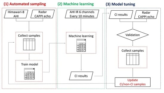
3.1. The Proposed Framework

The overall process of the proposed framework is described in Figure 1. As mentioned above, there are three major processes: (1) The automated sampling tool, (2) machine learning-based CI modelling, and (3) repeated model tuning through the validation. The following sections from Section 3.2, Section 3.3 and Section 3.4 are organized following those three main processes, consistent with Figure 1. One of the advantages of machine learning approaches is that, in contrast to static thresholding approaches, they can be optimized by updating training data. Using validation results to update the training dataset, the suggested framework can be improved by adjusting any misclassifications, thereby reducing false alarms.

3.2. The Automated Sampling Tool

The automated sampling tool automatically extracts the interest fields of CI and non-CI before the first CI events identified from ground radar data (Figure 2). First, areas with the first ≥35 dBZ occurrence from the weather radar echoes were collected considering the area, duration, and $T_b$ from the 11.2 µm channel images. Since not all radar echoes over 35 dBZ are caused by convective clouds, radar echoes with 253.15 K < $T_b$(11.2) µm < 288.15 K were excluded to remove unwanted radar echoes originating from non-convective clouds or already matured clouds based on empirical tests and previous studies [13,14,25,26]. After filtering, radar ≥35 dBZ points were used as initial seed points for region growing to find the cloud objects in the 10 min preceding CI. The basic idea of the region growing algorithm is to examine the adjacent pixels and decide whether to include them into the region of the seed point iteratively. The detailed process is as follows:

• First, a certain seed point (pixel A) is solely assigned to a region R.
• Four neighboring points (up, down, left and right) of the pixel A are added to the candidate pixel list.
• The differences of $T_b$(11.2) µm between the mean of region R and each point in the candidate list are calculated.
• The pixel with the minimum difference (e.g., pixel B) amongst the candidate points is added to the region R, and the mean temperature of the region R is updated.
• Neighboring pixels of the pixel B are added to the candidate pixel list.
• Repeat steps 3–5 until the minimum difference exceeds the threshold (here, 1.5 K).

When the region growing process is finished in the 10 min prior to CI (i.e., t₀), interest fields are collected from the cloud objects, and points of the minimum temperature of the cloud objects are used as new seed points for region growing 20 min before t₀. This process is repeated until clouds are not detected. By this iterative process, cloud objects can be tracked without the atmospheric motion vector (AMV), which is only available over cloud-free areas. Even if manual interpretation of the candidate CI samples is needed in the final step due to cases where the satellite and radar data do not match, this sampling tool saves a considerable amount of time and effort when building a database for the machine learning-based CI modelling.

3.3. Machine Learning-Based CI modelling

Before running the CI model, a cloud mask was adopted to eliminate areas of the clear sky, cirrus cloud, or matured cloud. Cirrus contamination has a particularly profound negative effect on the performance of CI detection [8,13,14,26]. Therefore, cloud masking focusing on removing cirrus clouds with the selected thresholds for brightness temperature was used based on Lee et al. [6] and cloud masking criteria from KMA as follows:

$$T_b\left(11.2\right)\mathsf{\mu }\mathrm{m}<253.15\mathrm{K}$$

(1)

$$T_b\left(11.2\right)\mathsf{\mu }\mathrm{m}-T_b\left(12.3\right)\mathsf{\mu }\mathrm{m}>6\mathrm{K},$$

(2)

$$T_b\left(6.2\right)\mathsf{\mu }\mathrm{m}-T_b\left(11.3\right)\mathsf{\mu }\mathrm{m}<-38\mathrm{K}.$$

(3)

Euation (1) was used to mask out matured clouds, and Equations (2) and (3) were used for masking out cirrus clouds using the difference of water vapor and IR channels.

To build a dataset for the machine learning-based model, 18 CI occurrence dates were selected from 2015 to 2017 (

Table 3. The list of CI cases used in this study.

Group	ID	Date	Usage	Model Tuning With
A	CI-A1	01 August 2015	Training dataset	-
	CI-A2	01 September 2015
	CI-A3	30 June 2016
	CI-A4	06 July 2016
	CI-A5	17 May 2017
	CI-A6	25 June 2017
	CI-A7	25 July 2017
	CI-A8	07 August 2017
	CI-A9	17 August 2017
B	CI-B1	24 May 2017	Test & tuning dataset	C+D
	CI-B1	05 July 2017
	CI-B1	10 August 2017
C	CI-C1	18 June 2017	Test & tuning dataset	B+D
	CI-C2	02 August 2017
	CI-C3	11 August 2017
D	CI-D1	28 June 2017	Test & tuning dataset	B+C
	CI-D2	30 July 2017
	CI-D3	16 August 2017

). In order to evaluate the developed model, samples were separated into four groups—one training and three test groups. Samples in the same CI occurrence date were not divided between groups, so the CI occurrence dates were separated exclusively for the independence of training and test cases. Group A was used as the training dataset, while Groups B, C, and D were used as the test datasets. Moreover, each test group was used for tuning the model of other test groups. When Group B was used as the test case, for example, Group A was used as the base training dataset while Groups C and D were used as the tuning dataset.

RF was adopted as the machine learning approach in this study because it has shown robust performance and the explainable ability for the results of many classification and regression studies in remote sensing [27,28,29,30,31,32,33,34,35]. RF has been used in the previous studies of CI detection with other machine learning approaches [6,9,15]. While RF is implemented in various programing languages, we used Fortran [27] in this study, which is widely used in operational systems in meteorological fields (the Fortran code is available at https://www.stat.berkeley.edu/~breiman/RandomForests/cc_home.htm).

RF creates a collection of trees based on Classification and Regression Trees (CARTs), which are rule-based decision trees [27]. A CART uses a recursive binary split approach to extract patterns or rules from training data. In RF, each CART grows using two randomizations in selecting samples and split variables to overcome the limitations of CARTs—the dependency on a single tree and high sensitivity to training samples. RF randomly permutes the values of each variable using the leave-one-out method and applies them to the tree and subtracts the number of correct cases in the variable-permuted data from the correct class in the untouched data. One of the advantages of RF is that it provides the mean decrease accuracy which can be interpreted as the relative variable importance. A variable with high mean decrease accuracy can be interpreted as an important and contributing variable in the RF model, degrading the accuracy when the variable is randomly perturbed. Through the empirical testing, the performance was found to improve asymptotically near the 250 trees, and thus the number of trees was set to 250 considering both performance and efficiency. Default values were used for the remaining parameters such as the number of variables sampled at each split node (squareroot of the number of variables) and the minimum node size of 1. The computational time for training the RF model was less than 30 s using Intel(R) Core i7-4770 CPU @3.40GHz.

There is a possibility that pixel-wise CI detection could make an inconsistent result over a CI region with salt-and-pepper noise. To mitigate this problem, majority voting and region growing methods were applied as post-processing based on Lee et al. [6]. These two post-processing approaches effectively reduce false alarms and increase the probability of detection by removing salt-and-pepper noise and making CI objects more compact and aggregated [6]. In this study, a 3 × 3 window was adopted for the majority voting process, and $T_b$(11.2) µm was used as the background for region growing with a 1.5 K threshold.

3.4. Model Tuning Throught the Validation

As denoted in the previous section, the validation of the model was conducted for Groups B, C, and D. For each test CI case, results at a certain time were compared with the time series of all radar echoes within 120 min. When the model predicted CI at the certain pixel with a 10 km buffer, the occurrence of radar echo over 35 dBZ within 120 min was assigned as a hit (H), while the non-occurrence of the radar echo over 35 dBZ was assigned as a false alarm (F). In a similar way, the validation result was assigned as a miss (M) when the radar echo exceeded 35 dBZ within 120 min without a CI result. No radar over 35 dBZ and no estimated CI resulted in a correct negative (C). The radar echoes from already matured or non-convective clouds were excluded during the validation process using convective cloud masking thresholds to focus on the convective clouds. After getting the validation result, the typical skill scores of the probability of detection (POD) and false alarm rate (FAR) were calculated as followed:

POD = H/(H + M)

(4)

FAR = F/(H + F)

(5)

From the validation result, model tuning was conducted to improve the machine learning-based model. As described in Figure 1c, hits and misses were added to the CI samples and the false alarms and correct negatives were added to the non-CI samples. The model tuning process was conducted for each group. For example, the validation results of Groups C and D were used to update the training dataset for Group B. This simple and intuitive process updated the dataset for each validation case, and the update of dataset resulted in the update of the machine learning model. Even if this process is one of the strong advantages of machine learning approaches, it has not yet been covered in studies on machine learning-based CI detection [6,9,15].

4. Results and Discussion

4.1. Temporal Trend of Automated Collected Samples

To understand how the temperature of the collected CI samples changes during the development of clouds, the time series variation of $T_b$(11.2) µm was analyzed with the entire set of collected samples. Figure 3 shows the temporal variation of $T_b$(11.2) µm measured from a total of 16,937 CI samples collected by the automated sampling tool. The averaged $T_b$(11.2) µm varies from 281.15 K to 271.39 K in 10–100 min before CI occurrence. This shows a similar pattern to a previous study of CI using Himawari-8 AHI over southern-east China [14]. When the radar CAPPI echo started to exceed 35 dBZ, the mean temperature of $T_b$(11.2) µm was 268.05 K, then it decreased rapidly to 247.18 K right after 10 min. When considering only the 30 min before and after CI events, convective clouds grew rapidly after the CI event with a −14.25 K cooling rate per 10 min, while the cooling rate was much smaller with −1.76 K per 10 min prior to the CI event. The mean standard deviation of $T_b$(11.2) µm was 4.64 K before the CI event, 7.30 K at the CI event, and 13.40 K after the CI event. Due to the variety in the duration and uplift power of each cloud in the developing phase, the standard deviation of $T_b$(11.2) µm was higher after the CI events compared with the pre-developing phase.

4.2. Variable Importance

The mean decrease accuracy from the RF model could be interpreted as being the relative importance in the RF model (Figure 4). Amongst the 12 interest fields, $T_b$(11.2) µm (cloud top temperature) showed the highest mean decrease accuracy. Previous studies using machine learning approaches also reported that $T_b$(11.2) µm representing cloud top temperature greatly contributed to classifying the CI event [6,9]. Variables of the $T_b$(8.6–11.2) µm (cloud-top glaciation) and $T_b$(6.2–7.3) µm trend (temporal changes in cloud-top height, updraft strength) were listed following $T_b$(11.2) µm. The $T_b$(8.6–11.2) µm was reported as the most significant variable among glaciation indicators in previous studies using PCA [12] and RF [6]. The updraft strength represented by the $T_b$(6.2–7.3) µm trend was also reported as the highest PCA rank for clouds with cloud-top temperatures ≥240 K [12]. In contrast, the $T_b$(6.2–7.3) µm trend was identified as a less contributing variable in RF [6], while the $T_b$ (8.6–11.2)–(11.2–12.3) µm trend resulted in the high mean decrease accuracy implying that the temporal changes in cloud-top glaciation were important for CI detection. As the overall distribution of the cloud-top temperature for the target clouds were higher in this study (~270–280 K) and Mecikalski et al. [12] (>240 K) than Lee et al. [6] (<240 K), the $T_b$(6.2–7.3) µm trend representing the updraft strength might be more significant than the trend of cloud-top glaciation at the early development of CI. Other trend variables except for the $T_b$(6.2–7.3) µm trend did not show high mean decrease accuracy. Interest fields of the temporal trend were more heterogeneous than interest fields at single times in an object (not shown here), thus large differences in the trend variables might exist within a single object. Thus, the averaged value over an object may be able to make a larger contribution of the trend variables for CI detection.

4.3. Model Performance

A quantitative evaluation of POD, FAR, and lead time was conducted for test CI cases and summarized by each group with and without the model tuning process (

Table 4. The score of the probability of detection (POD), false alarm rate (FAR), and lead-time for test Groups B, C, and D with and without model tuning.

Skill Score	Group B	Group C	Group D	Overall
POD (no tuning) POD (tuning)	0.72 0.78	0.92 0.89	0.73 0.79	0.79 0.82
FAR (no tuning) FAR (tuning)	0.48 0.39	0.39 0.28	0.52 0.44	0.46 0.37
Lead time in minutes (no tuning) Lead time in minutes (tuning)	49.5 38.4	37.5 36.1	45.0 36.6	44.0 37.0
Initial detect time in minutes (no tuning) Initial detect time in minutes (tuning)	71.6 65.6	52.7 55.9	75.1 59.7	66.4 60.4

). Without the tuning process (training dataset with only Group A), the overall skill scores were a POD of ~0.79, a FAR of ~0.46, and a lead-time of ~44.0 min. After the tuning process, the results for the POD and FAR were improved by 0.03 and 0.09. Overall, the POD slightly increased after tuning except for Group C. The POD increased slightly overall (~0.3), but increased by 0.6 for Groups A and C, suggesting that the model tuning process could improve the POD in some cases. However, the decrease in the POD for Group C implies that the tuning process did not always guarantee a better POD, hence it should be used carefully by considering the distribution of the CI cases used in the tuning process. With many more CI cases for tuning, a more stable tuning effect might be expected. For all test groups, the FAR was reduced by ~0.09. According to previous studies [8,14], lowering the false alarm rate is the most important and challenging problem in the CI modelling, which is expected to be mitigated through the model tuning process. In contrast to the POD and FAR, the lead-time was reduced from ~44 to ~37 min after the tuning process. Especially, the increase in the POD was accompanied by the decrease in the lead time in Groups B and D. As POD increased by ~0.08, the lead-time was shortened by ~10 min in both groups. The increased hits near the time of strong radar echoes (i.e., about 10–20 min prior to the time when rain starts to fall) might result in the lowered average lead time, but further study should be needed to explain the effect of model tuning over the lead time. In addition to lead-time, the initial detection time of CI was also examined to focus on the very first detection over each CI object. The initial detection time was defined as the maximum lead time of each CI case. Similar to the lead-time, the initial detection time of both Groups A and C was shortened by ~5–6 min while slightly extended ~3 min in Group B. Overall, the initial detection time became shorter ~6 min after the tuning process. Nonetheless, the initial detection time regardless of the tuning process reached ~ l h or even longer than that on average.

The direct comparison of the result from this study and previous studies using machine learning approaches is not appropriate due to the difference CI cases and reference data. Han et al. [15] resulted in a POD of ~0.75 and a FAR of ~0.45 with COMS MI data. Lee et al. [6] yielded a POD of ~0.80 and a FAR of ~0.20 using DT, RF, and LR from Himawari-8 AHI data over the Korean Peninsula. Although Lee et al. [6] yielded a higher performance than this study, it should be noted that the phase of target clouds is much less developed in this study (cloud top temperature ~265–285 K) than that of Lee et al. (~230–245 K). This indicates that the proposed approach in this study focuses on the much earlier detection of CIs than that in Lee et al. [6], which might increase the uncertainty of model forecasts. Consequently, the lead time and initial detection time identified in this study were longer than those in Lee et al. [6]. Mecikalski et al. [9] developed RF and LR models for CI detection using GOES-16 ABI and NWP data, yielding a POD of ~0.62 and a FAR of ~0.32 with only satellite data. Using both satellite and NWP data, Mecikaslki et al. [9] showed improved results with a POD of ~0.80 and a FAR of ~0.30. This implies that the NWP or other auxiliary data can be highly expected to increase the overall performance if adopted in the framework proposed in the present study.

Two case examples of CI-B2 and CI-C2 are depicted in Figure 5 and Figure 6. They show the predicted result of CI after the tuning process in the time series 20–50 min before the first occurrence of the target CI events, as well as the radar echo at that time. In Figure 5 (CI-B2), target CI events around the southern coast of the Korean Peninsula (marked with the black circle) were predicted around 50 min in advance. Around Jeju Island, located at 33.5°N and 127.5°E, scattered false alarms were found at the edge of a matured cloud (also in Figure 7). In the case of CI-C2 in Figure 6, target CI events around 35.5°N and 127°E were detected with 20–50 min of the lead time. As the time got closer to 04:50, the CI detection result became clearer.

The effect of model tuning on the CI detection performance was visually analyzed using validation maps in the cases of CI-B2 and CI-C2 (corresponding to Figure 5 and Figure 6) with time series depicted in Figure 7 and Figure 8. The top three figures (a–c) are validation maps without model tuning 30–50 min prior to the target CI events, while the bottom three figures (d–f) depict validation maps of the CI results after the tuning process. For both CI-B2 and CI-C2, false alarms were significantly reduced after model tuning. In Figure 7, false alarms over the inland area of the Korean Peninsula notably decreased, but there were more false alarms around the strong matured cloud near Jeju Island (33.5°N and 127.5°E) after the tuning process. The tuning dataset from the other groups (C and D for CI-B2) contributed to reducing the overall rate of false alarms, but there must have been some samples not suitable for CI and non-CI cases. This might be an inevitable problem due to the various meteorological conditions considering that only 18 days of CI occurrences were used in this study. In the case of CI-C2, the tuning process also significantly reduced the number of false alarms (Figure 8).

4.4. Novelty and Limitations

This study suggested the complete framework for machine learning-based CI detection, including an automated sampling tool and repeated model tuning process. These two sampling-related processes enhanced the advantages of using machine learning approaches, in terms of acquiring and updating the training dataset which has a significant effect on the performance of the developed model. By using the automated sampling tool, interest fields were collected not only prior to the CI events, but also after the CI events. With this backward and forward object tracking, a time series analysis was conducted to understand the development phase of convective clouds related to CI. The automated sampling tool used in this study can be helpful to generate a CI database over a new study area or period. Our machine learning-based model has a high dependency on the training dataset. When a misclassification occurs, the samples need to be updated to make the model mitigate the error. Although only 18 days of CI occurrences with four groups were tested in this study, the repeated model tuning continuously updated the training data to further improve model performance from an operational perspective. In other words, the suggested model tuning process can shore up the weak point of previous machine learning-based CI models. Even if there are some aspects that need to be examined further, this tuning process is expected to improve the performance of CI detection, especially in terms of decreasing the rate of false alarms. Moreover, several state of the art machine learning techniques, such as convolutional neural networks, could be easily adopted in this framework instead of RF. Consequently, the suggested framework is expected to help maintain the model from an operational point of view. Moreover, this framework can help to make a new CI detection model from scratch without a well-established database.

Despite the novelties of the proposed framework, however, there are still several limitations to solve after this study. The major difficulty in this study was to exclude unwanted radar echoes—i.e., those that were not CI events. Getting exact radar echoes for CI events is one of the most crucial processes in both the modelling and validation of CI detection. Previous GOES-based studies [9,10,25,36] used the −10 °C isotherm radar [19,20] over the US area. If isotherm −10 °C radar data were available, classifying radar echoes emanating only from CI would become easier, because strong convection generally starts from around −5 °C (Figure 3). As isotherm radar data was not available over the Korean Peninsula, this study used the radar CAPPI 1.5 km—the same as in the previous study [6]. The altitude of 1.5 km may not correspond to a −10 °C temperature, especially during the Korean summer with its very high humidity and surface air temperature, while the CI is generally defined by a radar ≥35 dBZ at the height of −10 °C. To get more accurate radar echoes from CI events, a combination of base and composite reflectivity could be examined in future work to compare the difference in the echoes between lower and higher altitudes.

5. Conclusions

A complete framework for detecting CI using Himawari-8 AHI over the Korean Peninsula was suggested in this study. The suggested framework consists of an automated sampling tool, machine learning-based model, and repeated model tuning. Without model tuning, the overall skill scores were 0.79, 0.46, and 44.0 min for the POD, FAR, and the lead-time, respectively. The model tuning resulted in better performance with an increase in the overall POD of 0.03 and a decrease to the FAR of 0.09. However, the lead-time and initial detection time slightly dropped by around 9 and 6 min, respectively. CI samples collected using the automated sampling tool showed the temporal distribution of convective clouds, with a cloud top temperature of ~268.05 K at the first occurrence of radar echo ≥35 dBZ. Amongst the 12 interest fields, the $T_b$(11.2) µm, $T_b$(8.6–11.2) µm, and $T_b$(6.2–7.3) µm trends were identified as the most important variables in the RF model, reflecting the importance of the cloud-top glaciation and temporal change in detecting CI. A visual comparison of the model tuning showed that there was a clear reduction in the rate of false alarms in cases of CI-B2 and CI-C2. Therefore, it is clear that the suggested framework is beneficial for effectively reducing false alarms.

To develop a robust and accurate CI detection model with machine learning approaches, a greatly expanded dataset reflecting various CI cases should be created. This process is challenging due to the complex meteorological conditions that CI events appear in. From this perspective, the proposed framework is promising and can be further improved in future work. Regarding model tuning, for example, the cross-tuning over different CI dates was conducted in this study. Time series model tuning within the same date in near real-time is also expected to improve the CI detection performance, as it is able to consider the temporal changes of the meteorological condition. Several state of the art machine learning techniques are also expected to bring better performance in the future. These techniques can easily be adopted in the suggested framework. Last but not least, the ability to accurately extract radar echoes only for CI events would be as significant as the CI modelling in the suggested framework. Therefore, further investigation into the relationship between the available radar data and CI is needed over the Korean Peninsula and East Asia.

References

1. Soriano, L.R.; de Pablo, F.; Díez, E.G. Relationship between Convective Precipitation and Cloud-to-Ground Lightning in the Iberian Peninsula. Mon. Weather Rev. 2002, 129, 2998–3003. [Google Scholar] [CrossRef]
2. Boccippio, D.J.; Cummins, K.L.; Christian, H.J.; Goodman, S.J. Combined Satellite-and Surface-Based Estimation of the Intracloud–Cloud-to-Ground Lightning Ratio over the Continental United States. Mon. Weather Rev. 2002, 129, 108–122. [Google Scholar] [CrossRef]
3. Vondou, D.A.; Nzeukou, A.; Kamga, F.M. Diurnal cycle of convective activity over the West of Central Africa based on Meteosat images. Int. J. Appl. Earth Obs. Geoinf. 2010, 12, S58–S62. [Google Scholar] [CrossRef]
4. Wang, C.-C.; Chen, G.T.-J.; Carbone, R.E.; Wang, C.-C.; Chen, G.T.-J.; Carbone, R.E. A Climatology of Warm-Season Cloud Patterns over East Asia Based on GMS Infrared Brightness Temperature Observations. Mon. Weather Rev. 2004, 132, 1606–1629. [Google Scholar] [CrossRef]
5. Mecikalski, J.R.; Bedka, K.M. Forecasting Convective Initiation by Monitoring the Evolution of Moving Cumulus in Daytime GOES Imagery. Mon. Weather Rev. 2006, 134, 49–78. [Google Scholar] [CrossRef] [Green Version]
6. Lee, S.; Han, H.; Im, J.; Jang, E.; Lee, M.-I. Detection of deterministic and probabilistic convection initiation using Himawari-8 Advanced Himawari Imager data. Atmos. Meas. Tech. 2017, 10, 1859–1874. [Google Scholar] [CrossRef] [Green Version]
7. Mecikalski, J.R.; Bedka, K.M.; Paech, S.J.; Litten, L.A. A Statistical Evaluation of GOES Cloud-Top Properties for Nowcasting Convective Initiation. Mon. Weather Rev. 2008, 136, 4899–4914. [Google Scholar] [CrossRef] [Green Version]
8. Walker, J.R.; MacKenzie, W.M., Jr.; Mecikalski, J.R.; Jewett, C.P. An Enhanced Geostationary Satellite-Based Convective Initiation Algorithm for 0-2-h Nowcasting with Object Tracking. J. Appl. Meteorol. Climatol. 2012, 51, 1931–1949. [Google Scholar] [CrossRef]
9. Mecikalski, J.R.; Williams, J.K.; Jewett, C.P.; Ahijevych, D.; LeRoy, A.; Walker, J.R. Probabilistic 0-1-h Convective Initiation Nowcasts that Combine Geostationary Satellite Observations and Numerical Weather Prediction Model Data. J. Appl. Meteorol. Climatol. 2015, 54, 1039–1059. [Google Scholar] [CrossRef]
10. Jewett, C.P.; Mecikalski, J.R. Adjusting thresholds of satellite-based convective initiation interest fields based on the cloud environment. J. Geophys. Res. Atmos. 2013, 118, 12–649. [Google Scholar] [CrossRef]
11. Zinner, T.; Mannstein, H.; Tafferner, A. Cb-TRAM: Tracking and monitoring severe convection from onset over rapid development to mature phase using multi-channel Meteosat-8 SEVIRI data. Meteorol. Atmos. Phys. 2008, 101, 191–210. [Google Scholar] [CrossRef] [Green Version]
12. Mecikalski, J.R.; MacKenzie, W.M., Jr.; König, M.; Muller, S. Cloud-Top Properties of Growing Cumulus prior to Convective Initiation as Measured by Meteosat Second Generation. Part II: Use of Visible Reflectance. J. Appl. Meteorol. Climatol. 2010, 49, 2544–2558. [Google Scholar] [CrossRef] [Green Version]
13. Merk, D.; Zinner, T. Detection of convective initiation using Meteosat SEVIRI: Implementation in and verification with the tracking and nowcasting algorithm Cb-TRAM. Atmos. Meas. Tech. 2013, 6, 1903–1918. [Google Scholar] [CrossRef]
14. Zhuge, X.; Zou, X. Summertime convective initiation nowcasting over southeastern China based on Advanced Himawari Imager observations. J. Meteorol. Soc. Jpn. Ser. II 2018, 96, 337–353. [Google Scholar] [CrossRef]
15. Han, H.; Lee, S.; Im, J.; Kim, M.; Lee, M.-I.; Ahn, M.H.; Chung, S.-R. Detection of convective initiation using Meteorological Imager onboard Communication, Ocean, and Meteorological Satellite based on machine learning approaches. Remote Sens. 2015, 7, 9184–9204. [Google Scholar] [CrossRef]
16. Harris, R.J.; Mecikalski, J.R.; MacKenzie, W.M., Jr.; Durkee, P.A.; Nielsen, K.E. The Definition of GOES Infrared Lightning Initiation Interest Fields. J. Appl. Meteorol. Climatol. 2010, 49, 2527–2543. [Google Scholar] [CrossRef] [Green Version]
17. Zinner, T.; Forster, C.; de Coning, E.; Betz, H.D. Validation of the Meteosat storm detection and nowcasting system Cb-TRAM with lightning network data—Europe and South Africa. Atmos. Meas. Tech. 2013, 6, 1567–1583. [Google Scholar] [CrossRef]
18. Müller, R.; Haussler, S.; Jerg, M.; Heizenreder, D. A Novel Approach for the Detection of Developing Thunderstorm Cells. Remote Sens. 2019, 11, 415–443. [Google Scholar] [CrossRef]
19. Lakshmanan, V.; Smith, T.; Hondl, K.; Stumpf, G.J.; Witt, A. A real-time, three-dimensional, rapidly updating, heterogeneous radar merger technique for reflectivity, velocity, and derived products. Weather Forecast. 2006, 21, 802–823. [Google Scholar] [CrossRef]
20. Stumpf, G.; Lakshmanan, V.; Smith, T.; Stumpf, G.; Hondl, K. The Warning Decision Support System-Integrated Information. Weather Forecast. 2007, 22, 596–612. [Google Scholar] [CrossRef]
21. Bessho, K.; Date, K.; Hayashi, M.; Ikeda, A.; Imai, T.; Inoue, H.; Kumagai, Y.; Miyakawa, T.; Murata, H.; Ohno, T.; et al. An Introduction to Himawari-8/9 New-Generation Geostationary Meteorological Satellites. J. Meteorol. Soc. Japan. Ser. II 2016, 94, 151–183. [Google Scholar] [CrossRef]
22. Da, C. Preliminary assessment of the Advanced Himawari Imager (AHI) measurement onboard Himawari-8 geostationary satellite. Remote Sens. Lett. 2015, 6, 637–646. [Google Scholar] [CrossRef]
23. Kurihara, Y.; Murakami, H.; Kachi, M. Sea surface temperature from the new Japanese geostationary meteorological Himawari-8 satellite. Geophys. Res. Lett. 2016, 43, 1234–1240. [Google Scholar] [CrossRef]
24. Yumimoto, K.; Nagao, T.M.; Kikuchi, M.; Sekiyama, T.T.; Murakami, H.; Tanaka, T.Y.; Ogi, A.; Irie, H.; Khatri, P.; Okumura, H.; et al. Aerosol data assimilation using data from Himawari-8, a next-generation geostationary meteorological satellite. Geophys. Res. Lett. 2016, 43, 5886–5894. [Google Scholar] [CrossRef]
25. Cintineo, J.L.; Pavolonis, M.J.; Sieglaff, J.M.; Heidinger, A.K. Evolution of Severe and Nonsevere Convection Inferred from GOES-Derived Cloud Properties. J. Appl. Meteorol. Climatol. 2013, 52, 2009–2023. [Google Scholar] [CrossRef]
26. Berendes, T.A.; Mecikalski, J.R.; MacKenzie, W.M., Jr.; Bedka, K.M.; Nair, U.S. Convective cloud identification and classification in daytime satellite imagery using standard deviation limited adaptive clustering. J. Geophys. Res. 2008, 113, 909. [Google Scholar] [CrossRef]
27. Breiman, L. Random forests. Mach. Learn. 2001, 45, 5–32. [Google Scholar] [CrossRef]
28. Guo, Z.; Du, S. Mining parameter information for building extraction and change detection with very high-resolution imagery and GIS data. GIScience Remote Sens. 2017, 54, 38–63. [Google Scholar] [CrossRef]
29. Sonobe, R.; Yamaya, Y.; Tani, H.; Wang, X.; Kobayashi, N.; Mochizuki, K. Assessing the suitability of data from Sentinel-1A and 2A for crop classification. GIScience Remote Sens. 2017, 54, 918–938. [Google Scholar] [CrossRef]
30. Richardson, H.J.; Hill, D.J.; Denesiuk, D.R.; Fraser, L.H. A comparison of geographic datasets and field measurements to model soil carbon using random forests and stepwise regressions (British Columbia, Canada). GIScience Remote Sens. 2017, 54, 573–591. [Google Scholar] [CrossRef]
31. Sim, S.; Im, J.; Park, S.; Park, H.; Ahn, M.; Chan, P. Icing Detection over East Asia from Geostationary Satellite Data Using Machine Learning Approaches. Remote Sens. 2018, 10, 619–631. [Google Scholar] [CrossRef]
32. Kim, M.; Im, J.; Park, H.; Park, S.; Lee, M.I.; Ahn, M.H. Detection of tropical overshooting cloud tops using himawari-8 imagery. Remote Sens. 2017, 9, 685. [Google Scholar] [CrossRef]
33. Forkuor, G.; Dimobe, K.; Serme, I.; Tondoh, J. Landsat-8 vs. Sentinel-2: Examining the added value of sentinel-2′s red-edge bands to land-use and land-cover mapping in Burkina Faso. GIScience Remote Sens. 2018, 55, 331–354. [Google Scholar]
34. Zhang, C.; Smith, M.; Fang, C. Evaluation of Goddard’s LiDAR, hyperspectral, and thermal data products for mapping urban land-cover types. GIScience Remote Sens. 2018, 55, 90–109. [Google Scholar] [CrossRef]
35. Liu, T.; Abd-Elrahman, A.; Morton, J.; Wilhelm, V. Comparing fully convolutional networks, random forest, support vector machine, patch-based deep convolutional neural networks for object-based wetland mapping using images from small unmanned aircraft system. GIScience Remote Sens. 2018, 55, 243–264. [Google Scholar] [CrossRef]
36. Sieglaff, J.M.; Cronce, L.M.; Feltz, W.F.; Bedka, K.M.; Pavolonis, M.J.; Heidinger, A.K. Nowcasting Convective Storm Initiation Using Satellite-Based Box-Averaged Cloud-Top Cooling and Cloud-Type Trends. J. Appl. Meteorol. Climatol. 2011, 50, 110–126. [Google Scholar] [CrossRef]
Figure 1. An overall flowchart of this study. The suggested framework is composed as follows: (a) The automated sampling tool; (b) machine learning-based CI modelling; (c) model tuning through validation. ML in (a,b) stands for machine learning.
Remotesensing 11 01454 g001
Figure 2. The process of the automated sampling tool. From the right to left side, the backward cloud object tracking was conducted using the region growing method. Starting with the seed points from radar constant altitude plan position indicator (CAPPI) echo ≥35dBZ area, seed points were updated iteratively. t0 is the time when rain starts to fall.
Remotesensing 11 01454 g002
Figure 3. The variation of T b (11.2) µm over the CI area from the samples obtained by the suggested automated sampling tool. Negative time differences in the x-axis refers to the time before the CI events, and the positive time difference represents after the CI events.
Remotesensing 11 01454 g003
Figure 4. The mean decrease accuracy of 12 interest fields in the RF model using all samples (Groups A, B, C, and D). A higher mean decrease accuracy is interpreted as indicating a more significant variable in the random forest (RF) model.
Remotesensing 11 01454 g004
Figure 5. Time series of CI detection results (ad) and radar CAPPI echoes (e,f) on 05 July 2017 (CI-B2) from 04:30 to 05:20 after model tuning. In (ad), the predicted CI area is shown in red with T b (11.2) µm as a background. The area over the target CI events is marked with a black circle in (e,f). The first ≥35 dBZ of radar echo over the target CI events occurred at 05:20 (f).
Remotesensing 11 01454 g005
Figure 6. Time series of CI detection results (ad) and radar CAPPI echoes (e,f) on 02 August 2017 (CI-C2) from 04:00 to 04:50 after model tuning. In (ad), the predicted CI area is shown in red with T b (11.2) µm as a background. The area over the target CI events is marked with a black circle in (e,f). The first ≥35 dBZ of radar echo over the target CI events occurred at 04:50 (f).
Remotesensing 11 01454 g006
Figure 7. The spatial validation map of CI-B2 30–50 min prior to the target CI events on 05 July 2017 05:20 (corresponding to Figure 5). Results without (ac) and with (df) model tuning were depicted with the same time series. FA and CN stand for a false alarm and correct negative, respectively. Note that the accuracy of the radar data could be degraded over the sea far from the inland area.
Remotesensing 11 01454 g007
Figure 8. The spatial validation map of CI-C2 30–50 min prior to the target CI events on 02 August 2017 04:50 (corresponding to Figure 6). Results without (ac) and with (df) model tuning were depicted with the same time series. FA and CN stand for a false alarm and correct negative, respectively. Note that the accuracy of the radar data could be degraded over the sea far from the inland area.
Remotesensing 11 01454 g008