1. Introduction
It is necessary to adopt more efficient mechanisms in agricultural monitoring to identify vulnerable regions in crops, for the purpose of avoiding economic losses [
1]. Remote sensing products have become significant in this matter, since they help with the monitoring of large areas and the identification of crop conditions in a systematic and fast way [
2]. These products also allow the estimation of important biophysical parameters for decision-making [
3,
4,
5,
6].
There are several satellites that are able to successfully monitor the development of crop phenological cycles in agricultural fields [
7]. However, there is no satellite, at least with free access, that can monitor the daily temporal frequency and with enough surface detail for farm-level analysis [
8]. In order to obtain images with daily frequency and spatial detail, the use of intercalibrations between orbital sensors [
9], along with fusion techniques of images from satellites with complementary spatial and temporal characteristics [
10,
11,
12], have been utilized.
Despite the adoption of the above-mentioned techniques [
13,
14], a factor that interferes in the use of orbital sensors in agricultural monitoring is cloud cover. This factor makes the continuous temporal monitoring of the vegetation impractical, and opens up opportunities for techniques involving radar sensors [
15]. Studies based on radar images are becoming ever more popular, and consequently have also been included in agricultural monitoring studies [
16]. Radar information may replace or at least complement techniques developed for optical sensors, such as vegetation monitoring with the normalized different vegetation index (NDVI) [
15], which is the most used index in the literature for such a goal [
17].
Active sensors that emit and capture radiation relative to microwave wavelengths do not suffer interference from particles present in the atmosphere, resulting in images free of the effects of clouds [
18]. In this context, the Sentinel 1 constellation has a C-band synthetic aperture radar (SAR) system, based on the systems already constructed in ERS-1 (European Remote Sensing-1), ERS-2 (European Remote Sensing-2), Envisat, and Radarsat. This constellation has a high spatial resolution and high temporal frequency [
16,
19] when compared with its predecessors [
20,
21].
The Sentinel 1 constellation has two satellites, Sentinel 1A and Sentinel 1B, which operate in the same orbit and have the same settings. The presence of both platforms distanced by 180° in the same orbit doubles its temporal frequency. This results in a frequency of images of 12 days for one satellite and six days for the constellation [
20,
21], with a 10-meter spatial resolution in the ground range detected products [
22,
23,
24]. Thus, the Sentinel 1 constellation expanded the possibilities for the application of data acquired by active sensors [
21], allowing the application of SAR data in monitoring the temporal dynamics of agricultural crops [
15,
16,
21].
The high sensitivity of electromagnetic waves from microwave length in relation to soil and vegetation water content, along with other random noise, makes them a challenge to work with, and to extract information related to vegetation in this spectrum [
16]. Despite the obstacles, researchers have glimpsed the advantages of working with radar data to solve cloud cover problems in vegetation monitoring [
25]. Studies carried out by Navarro et al. [
19] demonstrate a high correlation between time series of the NDVI and the backscatter of active sensors for agricultural crops. This result demonstrates that optical data can be replaced by SAR data in the presence of clouds. Frison et al. [
25] demonstrated that there is a strong relationship between the backscatter coefficients of Sentinel 1 (VV and VH polarities) and vegetation phenologies derived from the NDVI with the Landsat-8 satellite. Vreugdenhil et al. [
16] found the relationship between backscatter coefficients, as well as the ratio between them, with crop data. They concluded their research by highlighting the potential demonstration of radar image indices in vegetation monitoring.
Based on the great potential of Sentinel 1, and in terms of the relevant problem related to high cloud cover, it is necessary to search for alternative monitoring solutions that completely resolve the lack of information about the cultures in seasons with a high frequency of clouds. In this context, the objective of this study was to generate a cloudless product (NDVInc) by modeling the vegetation condition represented by the NDVI of Sentinel 2, using the Sentinel 1 backscatter with different regression techniques. This study stands out from the previous ones in the sense that the model generated here will enable the monitoring of vegetation independently of optical sensors. However, as the product generated by the developed model is based on Sentinel 2, this information may also be coupled directly.
2. Materials and Methods
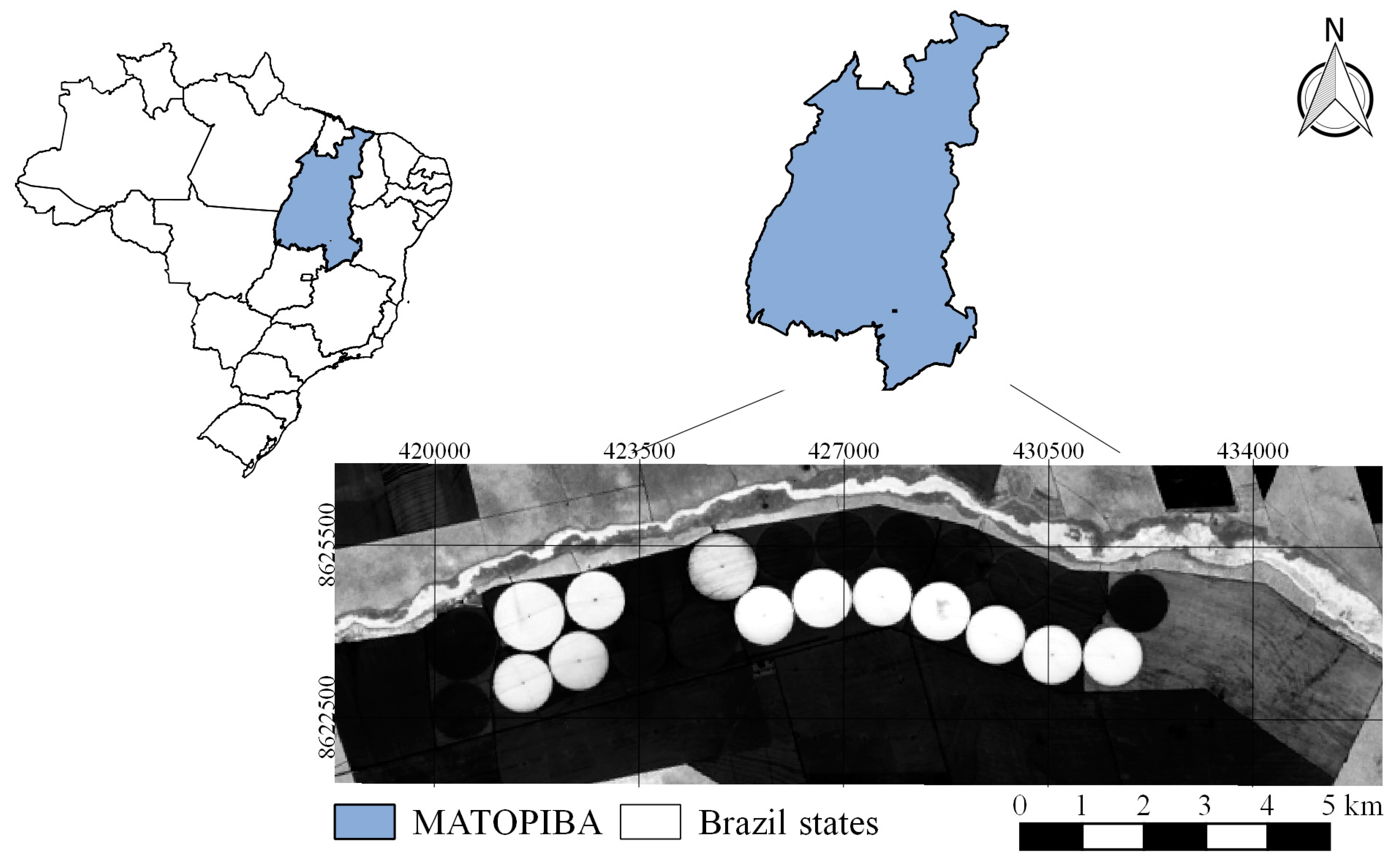
The study was carried out in an area of commercial agriculture located in the agricultural frontier denominated MATOPIBA, in the portion that belongs to the western mesoregion of the state of Bahia (
Figure 1). MATOPIBA is part of the states of Maranhão, Tocantins, Piauí, and Bahia. This region has a geographical reality different from the other regions of Brazil, characterized by the expansion of an agricultural frontier based on high productivity technology. The climate of a large part of the region (78%) is sub-humid tropical, especially in the central region of the territory [
26]. This region presents a complex variety of soils, with the presence of Latossolos (Ferralsols), Argissolos (Acrisols), and Neossolos Litólicos (Leptsols) being more frequent [
27].
The study area is delimited by the rectangle made by the left lower coordinate pair X1 = 416,840; Y1 = 8,627,100 and the upper right pair of coordinates X2 = 439,940; Y2 = 8,616,420, under the coordinate reference system Datum WGS-84, UTM (Universal Transverse Mercator) projection, zone 23S. The average altitude of the study area is 750 m in relation to the average sea level, with a flat relief according to the classes established by Embrapa [
27].
The study area has 17 central pivots, 16 of which are towable. The movement of the central pivots occurs only from one crop season to another—the equipment remains in the same area throughout the crop season. For this reason, irrigated areas are named “A” and “B” (
Figure 2). The study was carried out with soybean and maize sowed in the central pivots.
2.1. Field Data
In the study area, meteorological, irrigation, and crop data were collected, with the aim of guiding the interpretations generated in the modeling, since SAR data can be influenced by precipitation or irrigation [
16].
Meteorological data were collected near the central pivots by an automatic meteorological station (Davis, Vantage Pro Plus, Hayward, CA) belonging to the commercial property, located at the pair of coordinates X = 418,736.12 and Y = 8,621,573.48 (Datum WGS-84, projection UTM zone 23S). The meteorological station measures and stores daily data of air temperature (°C), wind speed (m s−1), solar radiation (W m−2), relative humidity (%), and rainfall (mm).
Sowing date, as well as irrigated depth data, and percentage of soil moisture in relation to field capacity (PSMFC), were provided by the commercial property along with the company (IRRIGER) responsible for irrigation management in the area of study.
2.2. Orbital Data
Data from the Sentinel 1 constellation (Sentinel 1A and 1B satellites) and data from the Sentinel 2 constellation (satellites 2A and 2B) were used. All the orbital data used were acquired from the Scientific Data Hub, maintained by the European Space Agency (ESA), at the link:
https://scihub.copernicus.eu/dhus/#/home.
The Sentinel 1A and 1B are satellites launched by ESA on April 3, 2014 and April 25, 2016, respectively [
19]. The images used from Sentinel 1 were all in the form of Interferometric Wide Swath Mode-IW with dual polarization (VV+VH), and were acquired under level 1 processing as ground range detected (GRD).
The Sentinel 2A and 2B platforms have a MultiSpectral Instrument (MSI) sensor, which captures the reflected radiation in 13 spectral bands [
28,
29]. Like the Sentinel 1A and 1B platforms, the Sentinel 2A and 2B platforms are also in the same orbit (with 180° lag from each other), a fact that increases the temporal frequency of Sentinel 2 images from 10 days (with one satellite) to five days.
The images from both constellations were selected for the days when the two platforms’ passages coincided in the study area. Images with 100% clouds were excluded before the orbital data processing step. During the observation period from 01 January 2016 until 17 August 2018 of both constellations, only four pairs of matching images were found to proceed with the calibration and validation phases of the models. These images refer to the dates: 24 June 2017, 21 December 2017, 20 April 2018, and 19 June 2018.
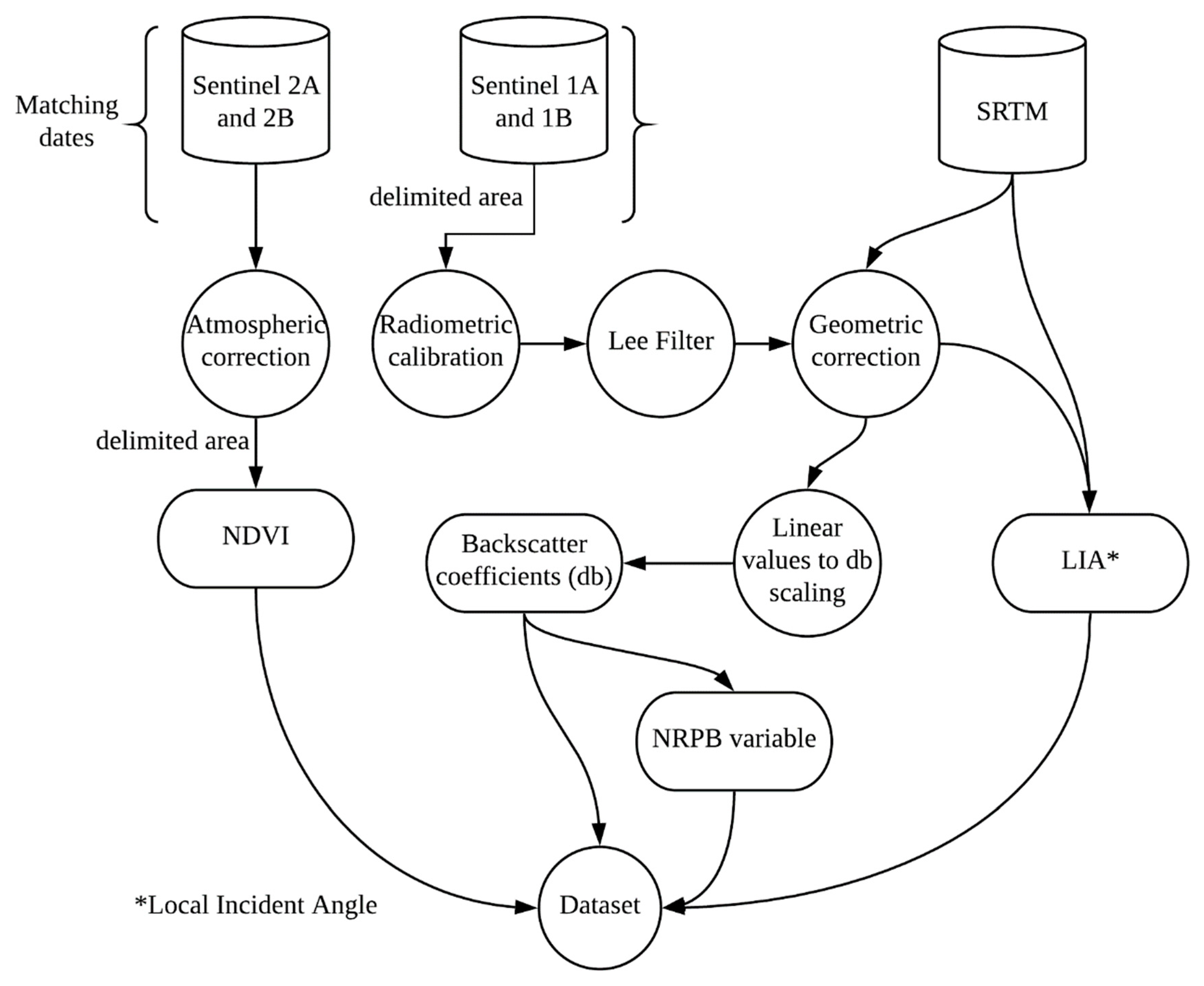
2.3. Orbital Data Processing
The methodology of the data processing was divided for the constellations of Sentinel 2 and Sentinel 1 (
Figure 3). The products generated for both constellations were used as inputs for the training and validation of the models. The same processing methodologies were applied for the temporal series of images, and are presented in the temporal analysis of the applicability of the model (
Section 2.6).
2.3.1. Sentinel 2 Image Processing
The images from the Sentinel 2 constellation were acquired at the processing level 1C, which already shows the values in reflectance at the top of the atmosphere, with only the conversion of these values to surface reflectance being necessary. Therefore, it was necessary to apply atmospheric correction to these images. For this, the DOS1 method, proposed by Chavez Jr. [
30], was applied.
After the atmospheric correction of the Sentinel 2 data, the surface reflectance obtained for the red and infrared bands were used to calculate the NDVI. The NDVI was calculated (Equation (1)) according to Rouse Jr. et al. [
31]:
where ρ
iv is the near infrared reflectance (band 8) and ρ
v is the reflectance corresponding to red (band 4).
The response amplitude of the NDVI ranges from −1.00 to 1.00, with negative values generally for clear water bodies, and values from 0.00 to 0.25 for exposed soil surfaces, which also can be the remains of straw. NDVI values between 0.25 and 0.40 represent soils with the presence of vegetation, and values above 0.40 represent vegetated surfaces. The closer the NDVI values are to 1.00, the stronger the vigor of the vegetation. For more information, consult Rouse Jr. et al. [
31]; Formaggio and Sanches [
32]; and Ponzoni et al. [
33].
After the processing of the Sentinel 2 images, we proceeded with the removal of pixels categorized as clouds. For this, we used the screen-based delineation classification methodology [
34], which is the manual selection of the clouds in the images.
Figure 4 represents the exclusion of clouds from the study area for the day 24 June 2018.
2.3.2. Sentinel 1 Image Processing
This step is necessary so that the SAR C-band from Sentinel 1 can be used in the prediction of the NDVI. All the processing of Sentinel 1 images from this study was realized in the Sentinel Application Platform, SNAP, using the Sentinel 1 toolbox [
35].
The first processing of the Sentinel 1 images was the radiometric calibration step, which allows the values of the images to be directly related to the backscatter of the surface [
36]. The radiometric calibration was applied according to Equation (2):
where σ
0i is the backscatter coefficient, A
i is the sigma calibration for each pixel (i), obtained from the calibration vector list (found in the calibration look-up tables, present in the image metadata), b is an constant offset (for GRD products), and DN
i2 is the digital number intensity [
19].
Before performing any analyses with the SAR images, it is necessary to reduce the speckle, which is one of the biggest noise sources in SAR data. Speckle is a random “salt and pepper” noise, which degrades the image data quality, as well as interfering in the understanding of backscatter responses from the surface features [
37]. To mitigate these interferences, we apply a spatial filter [
38]. The Lee filter with a 5×5 window was applied to the images to mitigate these effects [
36,
37]. The Lee filter is a particular case of the Kuan filter, which is based on the criterion of the mean minimum square error (MMSE) [
38].
Geometric corrections were also necessary because of the topographical variations of the scenes and the inclination of the radar sensor, which distort SAR images. This last fact is related mainly to the images that, in the moment of satellite passage, were not captured in the same direction of the nadir of the surface. Corrections of terrain, therefore, present mitigating measures to represent the surface in the most real way possible [
37]. Geometric distortions are not considered in GRD images from the ESA, and it is necessary to perform this procedure to improve the accuracy of the image geolocation. In order to perform this step, we applied the range doppler terrain correction, which used data from the digital elevation model SRTM (shuttle radar topography mission), with 1 arc-second of spatial resolution—approximately 30 m. This data was acquired automatically through SNAP, using the Sentinel 1 toolbox [
39].
The range doppler terrain correction procedure generated the local incident angle (LIA) product, which is the incident angle of the radiation in relation to the normal of each pixel of the surface. This variable was also used as a covariate in some of the approaches tested (A2 and A4, in
Section 2.4).
The last step of the Sentinel 1 processing was the conversion of the backscatter coefficients (σ
i0), which were in a linear scale, to decibel (db) scaling, according to Equation (3):
where σ
i0 (db) are the backscatter coefficient values in decibels.
After the processing steps for Sentinel 1, we proceeded with the calculation of the normalized ratio procedure between bands (NRPB). The NRPB was computed in order to generate a greater number of covariates to compose the input set of the models and to aid in the prediction of NDVI, as performed by Filgueiras et al. [
40]. This process was performed for the backscatter data of the VH and VV polarizations (Equation (4)):
where σVH and σVV are the backscatter VH and VV polarization, respectively. The NRPB was used to aid in the four approaches tested for prediction of NDVI, with the function of increasing the number of covariates.
2.4. Regression Algorithms and Approaches Used in NDVInc Modeling
Eight regression algorithms were used to find the one that best suits the NDVI data from Sentinel 2. The algorithms tested were: forward stepwise regression (lmStepAIC); random forest (rf); support vector machine regression—radial basis function kernel (svmRadial); support vector machine regression—linear kernel (svmLinear); Bayesian-regularized neural network (brnn); linear regression (lm); cubist; and gradient boosting machine (gbm). For more information about them, see the publication by Kuhn and Johnson [
41]. These methods were selected to encompass a variety of different regression models: linear regression and its derivatives (i); nonlinear regression models (ii); and regression tree- and rule-based models (iii) [
41].
Along with the regression algorithms, four approaches were tested in order to find the most pertinent for the modeling of NDVI
nc with Sentinel 1 data (
Table 1). The approaches varied according to the inputs derived from Sentinel 1, with the following functions being established:
2.5. Training and Validation
In order to proceed with the modeling of the NDVI
nc, we first made the spatial resolutions of the products generated in both constellations compatible, as well as adjusting the pixels of the products of one constellation in relation to another. This compatibilization was performed using the resample function of the “raster” package [
42] in the R software. Subsequent to this procedure, the raster data generated for both constellations were stacked per date used for modeling.
A total of 18,700 points was extracted from the central pivots in the four pairs of images used for the modeling, which were then separated into two groups according to Ayoubi et al. [
43]: training of the model (70%) and validation of the models (30%). The points were used to extract information regarding the NDVI of Sentinel 2, and information derived from Sentinel 1. The points were spatialized using randomized stratified sampling, ensuring that the information of one pixel was not extracted more than once on the pair of images.
In order to select the model with the highest performance in the prediction of NDVI
nc with Sentinel 1, the NDVI product derived from Sentinel 2 was used as observed data. The analysis of the model with the best performance was evaluated by two methodologies: cross-validation on the training set, and the prediction for the validation set (holdout). The cross-validation on the training set was the k-fold with 10 folds and 10 repetitions, generating later the absolute mean error (MAE), root mean square error (RMSE), and coefficient of determination (r
2) metrics. In the methodology using the validation set, the following statistical metrics were evaluated: r
2, RMSE [
44], Nash–Sutcliffe efficiency (NSE) [
45], mean bias error (MBE), and MAE, according to Equations (9)–(13), respectively. Cross-validation methodologies were applied because this helps demonstrate the degree of generalization of the models, being a widely used technique to perform model selection in prediction problems [
46].
where Pi is the value predicted by the model; Oi is the observed value of NDVI;
is the observed mean value and n is the number of data pairs. After the analysis of the results from the methodologies, the best model was chosen.
2.6. Temporal Analysis of the Applicability of the Model
After the development and choice of the most appropriate model, which used images that both platforms took on the same day, a simulation was performed during the 2017/2018 and 2018 harvests in the study area. This analysis was based on obtaining NDVInc using all the available images of the Sentinel 1 constellation (25 images) and the NDVI obtained by the Sentinel 2 constellation (55 images) during two crop seasons that extended from 02 October 2017 to 08 August 2018.
Soybean and maize were cultivated in the central pivots of the study area during the dates of the analysis. The temporal analysis using the best model was performed for the central pivots 1A and 13B (
Table 2).
In order to deepen in the temporal analyses carried out in the work and to understand what happened on the days of the images, emphasis was given to central pivot 1A. In
Table 3 we find information about the crop season of soybeans in the central pivot for the days of the images. This was a unique crop season for the central pivot 1A, which is why the dates in
Table 3 go from 26 November 2017 to 27 March 2018, corresponding to the first image after the sowing and the last image before the harvest of the soybean for this central pivot, respectively. According to field tests conducted by the company responsible for irrigation management, this central pivot had an irrigation efficiency of 86.9% at the time the images were taken.
To better understand the temporal analysis of the applicability of the models developed for the NDVI
nc product, we proceeded with natural color compositions of Sentinel 2 images to be able to visualize the presence of clouds on the dates (
Table 3).
3. Results
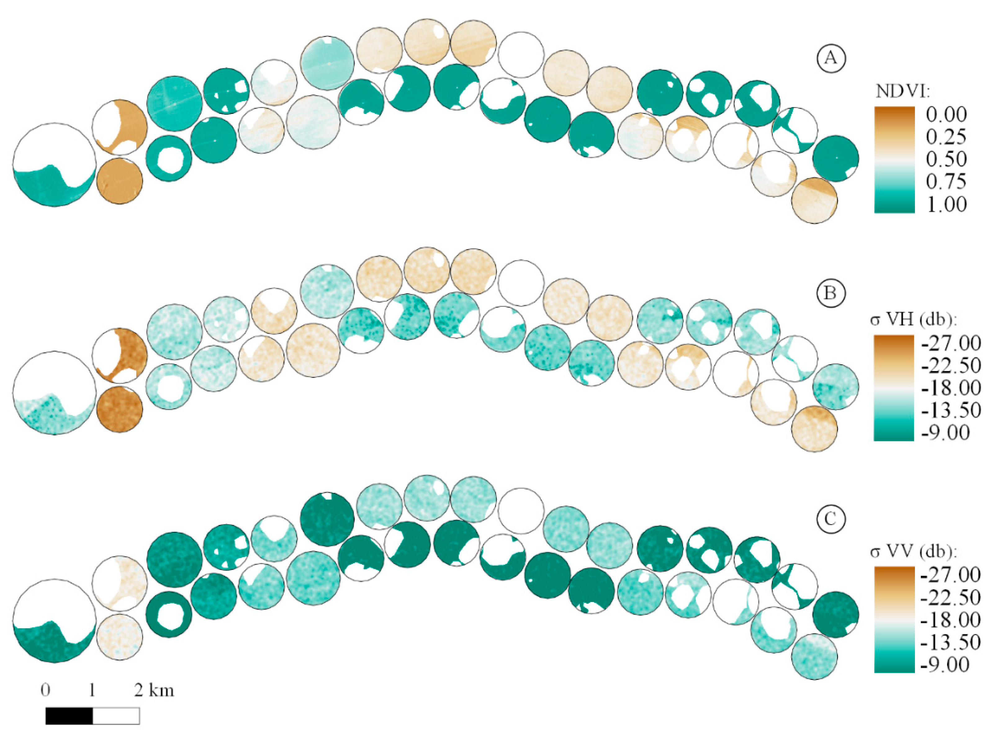
Figure 5 shows the images used to train the models for the day 24 June 2017. This set consists of an NDVI image of Sentinel 2 and the backscatter coefficients in the different polarizations of Sentinel 1. The backscatter coefficients σVH and σVV were used as inputs in all four approaches (
Table 1). Observing
Figure 5, the relationship between the backscatter coefficients and NDVI, or vegetation, is remarkable. It is possible to observe the vegetation variability at the central pivots by observing exclusively the dynamics of the values of the backscatter coefficients σVH and σVV.
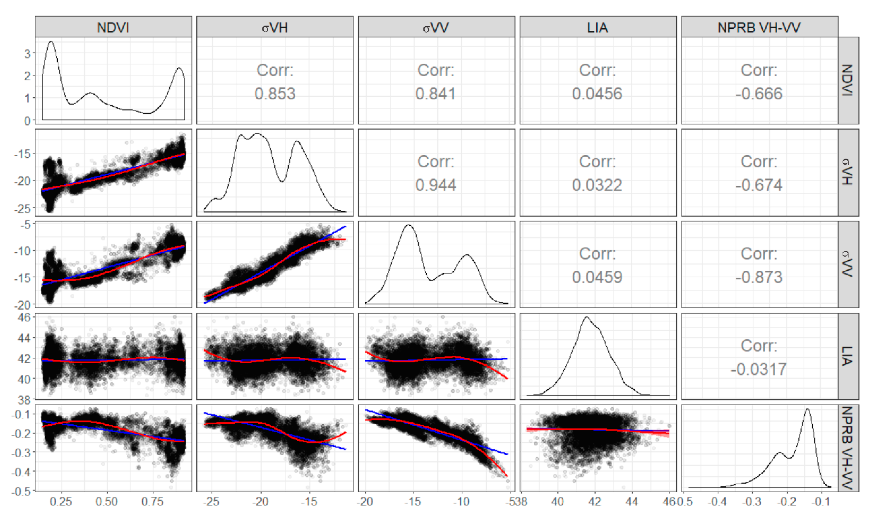
Correlations of the independent variables with NDVI are presented in
Figure 6 and
Figure 7, which have the objective of demonstrating the quantitative relationships between these variables. The correlations shown in
Figure 6 are valid for the A1 and A2 approaches, and those presented in
Figure 7 are valid for the A3 and A4 approaches.
In analyzing
Figure 6, it is noted that the number of values in which there are no linear backscatter responses to NDVI corresponds to the portions with the lowest NDVI values. These values are correspondents to the central pivots that had exposed soils and crop residues on the dates used for the modeling of NDVI
nc, a circumstance that reiterates the relation of the backscatter coefficient with other factors, such as soil moisture [
47]. This finding motivated the execution of approaches 3 and 4, for which correlations of the variables are shown in
Figure 7.
Comparing
Figure 7 with
Figure 6, it may be observed that the correlations of all the input variables increased substantially in relation to the NDVI. The fact that the correlation is higher when excluding NDVI values lower than 0.25 is due to the interaction of electromagnetic radiation of band C of Sentinel 1 with the soil. When the low values of the NDVI are excluded, abrupt changes in the values of the backscatter caused by the soil moisture variability are also excluded. Because of this, the correlations increase, since the NDVI does not capture these variations.
The LIA was added as an input variable in the A2 and A4 approaches because it is a parameter that represents the way that electromagnetic radiation reaches the surface. Thus, this variable may be related to the response intensities of the backscatter captured by the sensor [
6]. Therefore, it may assist in the attenuation of possible randomness of the responses in relation to the surface, as a non-Lambertian behavior in backscatter radiation for example.
Regarding the variable NRPB, it is possible to emphasize the relevance of it in the prediction, since this variable has a correlation with the NDVI that is considered moderate in the approaches A1 and A2 and strong in the approaches A3 and A4 (
Figure 6 and
Figure 7).
Figure 8 shows the results of the k-fold cross-validation performed with the training set used to model the NDVI
nc. The cross-validation is important to demonstrate the degree of robustness in which the modeling was performed, a fact that is noticeable for all the results of the approaches considering their low variability, as shown in
Figure 8. Note that in general, in all approaches, the linear-based models (lmStepAIC, lm, and svmLinear) presented with the worst performances.
The addition of the LIA variable presented a gain in performance when comparing the A1 approach (
Figure 8A) with A2 (
Figure 8B) and the A3 approach (
Figure 8C) with A4 (
Figure 8D). Approaches that excluded values less than 0.25 of the NDVI presented more assertive results for cross-validation. Independent of the approach used, the rf model was the one that presented the best results for the statistical metrics of cross-validation (
Figure 8). This circumstance makes the rf the model that has the greatest capacity for generalizations in this situation.
To help with choosing the best model, the metrics obtained in the validation set were also analyzed with the holdout technique. Thus,
Table 4 presents the statistical metrics obtained by each of the regression models for the validation set (holdout) in the different approaches. It is observed that, even with a set of separate points (validation set), these models had the ability to predict the variable of interest with metrics similar to those obtained in the cross-validation (
Figure 8), a fact that confirms the high capacity of these models in modeling the NDVI with Sentinel 1 data. Emphasis can be given to the rf algorithm, which achieved the best metrics again.
The developed rf models stood out among all the regression algorithms by performing best in all the approaches assessed. Therefore, we chose this algorithm to perform the temporal analysis of the NDVI
nc product. For the approaches considering only NDVI > 0.25 (A3 and A4), the model generated by lm (linear regression) presented a good fit, which could be an interesting option since it can be easily applied through a linear equation. Equations (14) and (15), developed by the lm for the approaches A3 and A4, could be used in different regions as long as the user is monitoring the same crops for which they were developed. If the coefficients do not fit well for predicting the NDVI in other regions, the equation parameters could be adjusted following the same methodology.
To help the readers understand the context of the temporal analysis, the meteorological variables for the study region in this period are presented (
Figure 9). Since they can influence the backscatter data, the conditions of the monthly maximum, average and minimum air temperatures (
Figure 9A), the variability of monthly relative humidity (
Figure 9B), the variability of monthly precipitation (
Figure 9C) and the sum of the monthly precipitation (
Figure 9D) are shown.
Therefore, when we analyzed
Figure 9, it can be observed that rainfall was concentrated between November 2017 and April 2018 (
Figure 9C,D) and, consequently, was when relative humidity reached its highest values (
Figure 9B). It is also during this period that the air temperature registered its smallest amplitudes between the minimum and maximum monthly averages (
Figure 9A).
In
Figure 10 we observe the temporal analysis of the NDVI
nc product for two central pivots of the agricultural property (P1A and P13B). In this analysis, the product NDVI
nc (red line) is plotted against the NDVI calculated through Sentinel 2 (green line). It may be seen in the same figure that NDVI
nc was responsive in capturing the development of the crop in the field for all approaches.
It was noticed when analyzing the two central pivots presented in
Figure 10 that, during the temporal analysis (02 October 2017 to 08 August 2018), there were several situations in which we could not make inferences about the vegetation through the analysis of the NDVI with Sentinel 2. This is because of the instability of the values of the NDVI (
Figure 10), which are directly related to the presence of clouds in the region. This situation is more prominent during the periods when rainfall events concentrate; in this case, from November 2017 to April 2018 (
Figure 9C,D).
In relation to the different approaches performed (
Table 1), it is noted that all of them were sensitive to changes in vegetation, as observed by the trend of NDVI
nc values presented in
Figure 10. However, it can be observed in
Figure 10, considering both the central pivots and all the approaches, that there is a high discrepancy of NDVI values in relation to NDVI
nc at some dates. This fact is notable for example in the second NDVI
nc image (03 November 2017) and the third NDVI
nc image (15 November 2017), which were represented by the second and third point in the NDVI
nc lines of all approaches of
Figure 10.
In order to better understand the applicability of the models and their reliability, the natural color compositions of the Sentinel 2 images of central pivot 1A are shown in
Figure 11. This figure shows the images from the first image after the sowing period of the soybean crop (26 November 2017) until the last image available before the end of irrigation management (26 March 2018). The period in which the irrigation management for central pivot 1A (20 November 2017 to 28 March 2018) was considered, registered a total of 836.90 mm of rainfall, 442.12 mm of ETrc (real crop evapotranspiration), 509.74 mm of ETo (reference evapotranspiration), and 38.33 mm of irrigation depth.
The persistent cloud cover during this crop season, presented in
Figure 11, is remarkable, since only two from 22 images captured by the Sentinel 2 were cloudless for central pivot 1A. The number of images with the presence of clouds reinforces the importance of the product obtained in this work, which obtained, along the soybean crop in central pivot 1A, a total of 11 images of NDVI
nc, increasing substantially the capacity of monitoring in cloudy regions.
4. Discussion
The responses from the SAR data are sensitive to changes in the surface moisture [
47], so if there is rainfall in the area, or even irrigation, it may be a factor that causes interference in the NDVI
nc modeling. When the crop is already in the closed canopy, the interference from the water content is lower, since the precipitated water, either from rain or the irrigation system, tends, by gravity, to go into the soil, reducing the interference in the capture of the backscattered radiation.
The electromagnetic radiation of the C-band does not have the capacity to cross-vegetated surfaces, as happens with the radiation of the L-band [
18]. Thus, electromagnetic radiation from Sentinel 1 will interact more strongly with the above ground cover. In this way, the reason for the C-band sensitivity to changes in the vegetation can be understood. However, if the soil is exposed or there are crop residues and straw, the backscatter may present a greater interaction with the soil, being very sensitive to the moisture present in the same. This fact is in agreement with the statement made in the study of Bousbih et al. [
47], which reports that the sensitivity of Sentinel 1 to soil moisture decreases with plant cover growth (NDVI). This reinforces the need to know the meteorological and irrigation conditions in the region where the data are acquired.
The responses captured by the backscatter in situations of bare soil is highly related to the dielectric constant of the largest component present in the soil pores (air or water) [
18], since the wavelength of the C-band will interact with the components of soil only in situations with low biomass (NDVI < 0.25).
The NRPB calculated in the present study is the normalized ratio of the backscatter coefficients. Therefore, a strong correlation with the ratio σVH/σVV is expected, which can explain the help that NRPB gave to the model, given the findings by Veloso et al. [
17]. These authors highlight the similarity found in the NDVI and σVH/σVV ratios with agricultural crops. In addition, there is also the fact that NRPB aggregates predictive information into the models tested, explaining facts that cannot be elucidated only with the backscatter information. The insertion of the NRPB variable in machine learning models, like rf, helps the results to reach better statistical metrics in the validations, and consequently leads to greater generalization capacity in the models [
48,
49], since these kinds of models are recognized for having a high capacity for pattern recognition and complex solutions [
6].
The findings of the validation metrics are in accordance with the review carried out by Sivasankar et al. [
6] on agricultural crops monitored by radar remote sensing, since the best algorithm selected in the present study was the rf (machine learning algorithm). The reviews of these authors point out that most studies involving this theme address three sets of models, with machine learning algorithms being one of them. They also point out that the best results achieved with the monitoring of cultures with SAR data come from machine learning techniques and, therefore, these are the most recommended methodologies to relate vegetation with SAR data.
The discrepancy in NDVI
nc and NDVI with respect to the second (03 November 2017) and third (15 November 2017) date of
Figure 10 is due to high cloud cover, which affects Sentinel 2 data, and precipitation, which affects the soil moisture and consequently affects the SAR data [
18,
50]. Based on the meteorological data acquired in the weather station, on 03 November 2017, rainfall of 1.6 mm occurred, and on the previous day there was a 4.6 mm occurrence. Regarding the date of 15 November 2017, there was no precipitation event on this day, however, during the previous two days there was rain of 22.8 mm (14 November 2017) and 32.6 mm (13 November 2017), explaining the relative discrepancy with the NDVI values. The large difference between the NDVI and NDVI
nc in these dates is mainly due to the fact that the area of the central pivots covered exposed soils during these periods, when only the area of central pivot 13B (
Table 2) was sown. [
17]
. After the canopy closure, there were no more abrupt changes in NDVI
nc (
Figure 10), as at that point the vegetation was responsible for the major changes in NDVI
nc values.
The A3 and A4 approaches, despite presenting cross-validation and validation set metrics that were higher than the A1 and A2 approaches, are less generalist, since they were not modeled with NDVI values for exposed soil and crop residues. This is noticeable, since the A3 and A4 approaches perform poorly when modeling events of low biomass. This fact is explicit in
Figure 10, in the passage from the first to the second crop season of central pivot 13B and in the fallow of central pivot 1A. This feature makes the A3 and A4 approaches suitable only for situations where crops are already undergoing vegetative development or in a complementary manner to NDVI data from Sentinel 2, since these may be directly related to it. Because NDVI
nc has been modeled based on the NDVI from Sentinel 2, these two products are directly associable.
Among the four approaches, the ones which incorporated LIA as one of the inputs presented higher validation metrics. Therefore, if any of the approaches have to be applied throughout the crop cycle, opting for a more general approach, such as the A2 approach, is preferred. However, if the idea is just to fill a date lost by clouds in which the crop has a closed canopy, the A4 approach is also recommended.
The sensitivity of the backscatter coefficient responses occurs mainly due to the strong relationship of these responses to the surface dielectric properties [
18]. It is suggested that studies related to the obtaining of surface parameters using radar need to consider events that alter the surface moisture in the interpretation of the data, due to the relationship of this variable with the SAR data [
22,
50,
51,
52]. Hence, it is important to know the meteorological information of the study area, so that inferences of the behavior of the NDVI
nc data can be made for temporal analysis [
17]. For instance, higher interferences of soil moisture in radar backscatter are expected for bare soil during the months with higher rainfall.
The temporal analysis is of extreme relevance, for it demonstrates the applicability of the model, emphasizing its temporal generalization capacity, which is in agreement with the findings of Veloso et al. [
17]. These authors assessed the relationship of the temporal behavior of agricultural crops using Sentinel 1 images and Sentinel 2-like images, correlating the backscatter coefficients and the σVH/σVV ratio with the NDVI. However, these authors did not create an NDVI model from the variables derived from Sentinel 1, as performed in the present research.
The real interest in generating NDVnc from Sentinel 1 products is to facilitate further crop analysis and monitoring, independent of cloud cover. The NDVInc makes it possible to estimate different biophysical parameters, such as the crop coefficient, leaf area index, and biomass of crops. Thus, it is possible to apply the NDVInc product to the same amount of analyses that can be carried out by the NDVI.
5. Conclusions
The data derived from Sentinel 1 provided great reliability in modeling the NDVI of agricultural crops throughout their phenological cycle. This fact is related to the correlation of backscatter coefficients from the σVH and σVV polarizations with the NDVI of agricultural crops. This proves the applicability of Sentinel 1 data to the continuous monitoring of agriculture in regions with frequent cloud cover.
Among the regression algorithms tested, the machine learning ones proved to be efficient in modeling the NDVI with data from Sentinel 1, especially the random forest (rf) model. This model was the most recommended to model the NDVInc in the conditions of the present research, independent of the approaches utilized.
From the approaches performed, all of them were sensitive to vegetation changes, but the A2 and A4 approaches, which make use of the LIA, should be highlighted. However, the methodology of the A2 approach is the most recommended, given the greater capacity of generalization in all the phenological phases, including the initial phase of the crops.
The high frequency of Sentinel 1 images, along with the information it produces from the surface, means that the monitoring of agricultural crops can be continuously carried out during any weather situation. This is concluded because Sentinel 1’s C-band does not have substantial influences on soil water content after the canopy closure of crops.

 ,
, 


